
Novel Hybrid Crayfish Optimization Algorithm and Self-Adaptive Differential Evolution for Solving Complex Optimization Problems

 ,
,  , and
, and
Abstract
1. Introduction
2. Problem Statement
2.1. Paper Contribution
- Novel hybrid optimization algorithm: We propose the Hybrid COASaDE optimizer, a strategic integration of the Crayfish Optimization Algorithm (COA) and Self-adaptive Differential Evolution (SaDE). This hybridization leverages COA’s explorative efficiency, characterized by its unique three-stage behaviour-based strategy, and SaDE’s adaptive exploitation abilities, marked by dynamic parameter adjustment. The novelty of this approach lies in the balanced synergy between COA’s broad search capabilities and SaDE’s fine-tuning mechanisms, resulting in an optimizer that excels at both exploration and exploitation.
- Enhanced balance between exploration and exploitation: The Hybrid COASaDE algorithm effectively addresses the balance between exploration and exploitation, a common challenge in optimization. It begins with COA’s exploration phase, which extensively probes the solution space to avoid premature convergence. As potential solutions are identified, the algorithm transitions to SaDE’s adaptive mechanisms, which fine-tune these solutions through self-adjusting mutation and crossover processes. This seamless transition ensures that the algorithm can robustly navigate complex high-dimensional landscapes while maintaining a balanced and effective search process throughout the optimization.
- Engineering applications: The applicability and effectiveness of the Hybrid COASaDE optimizer are validated through several engineering design problems, including welded beam, pressure vessel, spring, speed reducer, cantilever, I-beam, and three-bar truss designs. In each case, Hybrid COASaDE achieves high-quality solutions with improved convergence speeds. This demonstrates the optimizer’s versatility and robustness, making it a valuable tool for a wide range of engineering applications.
2.2. Paper Structure
3. Related Work
3.1. Overview of COA
3.2. Overview of Self-Adaptive Differential Evolution (SaDE)
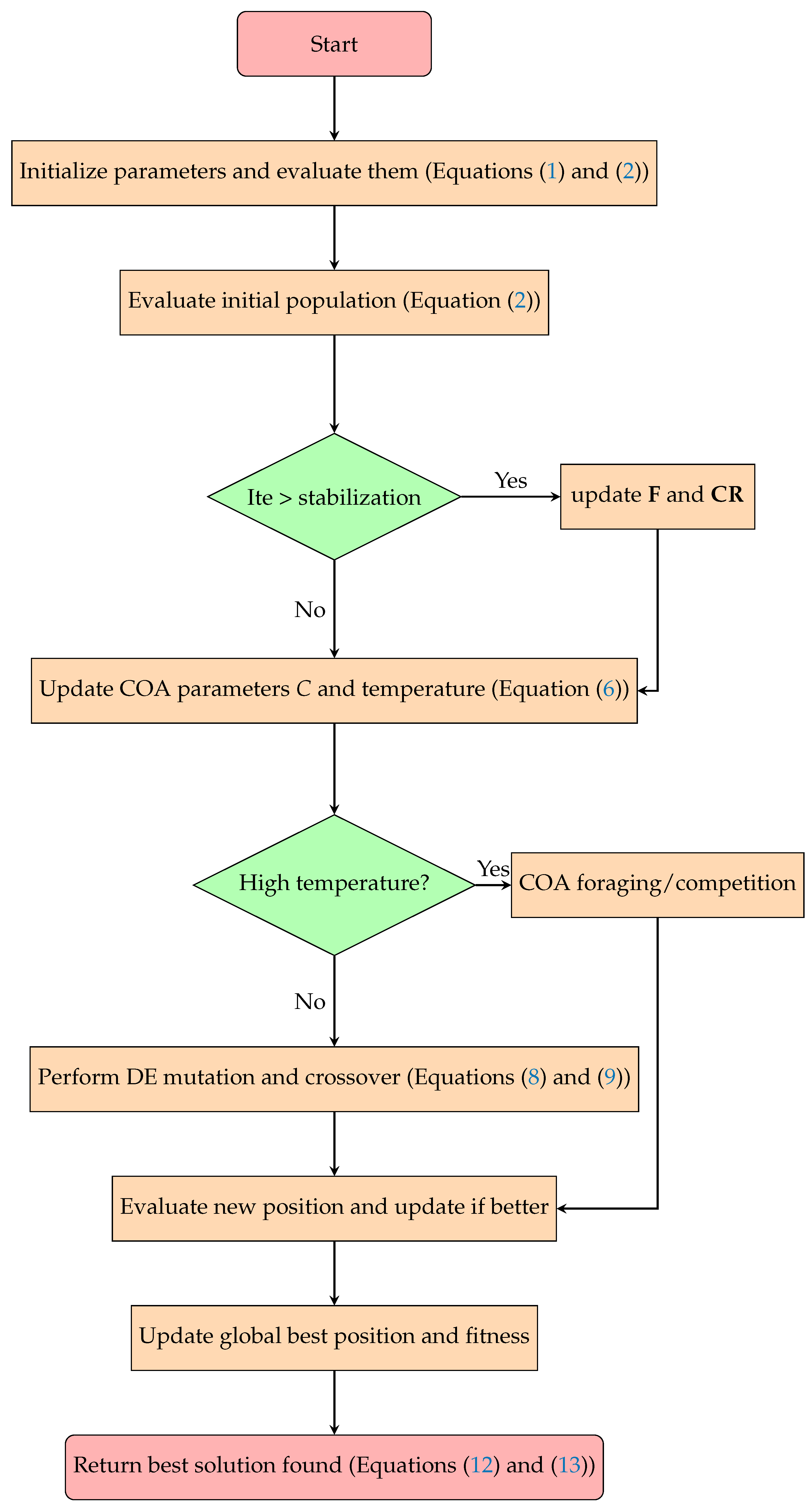
4. Hybrid COASaDE Optimizer
4.1. COASaDE Mathematical Model
- Population Initialization:
- 2.
- Evaluation:
- 3.
- Mutation Factor and Crossover Rate Initialization:
- 4.
- Adaptive Update:
- 5.
- COA Behavior:
- 6.
- SaDE Mutation and Crossover:
- 7.
- Selection:
- 8.
- Final Outputs:
| Algorithm 1 Pseudocode for the Hybrid COASaDE algorithm. |
|
4.2. Exploration Phase of Hybrid COASaDE
4.3. Exploitation Phase of Hybrid COASaDE
4.4. Solving Global Optimization Problems Using COASaDE
4.5. Symmetry in Hybrid COASaDE
4.6. Computational Complexity of COASaDE
4.7. Computational Components
- Initialization:The population X is initialized with N individuals (Equation (15)), where D is the dimensionality of the search space.
- Fitness evaluation:The fitness of each individual in X is evaluated, where M is the complexity of the objective function.
- Adaptive parameter updating:The adaptive parameters F and for individuals are periodically updated, typically at every tenth iteration beyond .
- COA and SaDE operations:This controls COA behaviors (Equation (18)) and alternative COA behaviors (if condition ).This controls SaDE mutation and crossover operations (Equation (19)).
- Boundary conditions and fitness updating:This is used to apply the boundary conditions.This is used to evaluate the fitness of mutated individuals.
- Termination:The algorithm runs for T iterations, with T directly influencing the total computational complexity.
5. Testing and Comparison
5.1. CEC2022 Benchmark Description
5.2. CEC2017 Benchmark Description
5.3. Configuration of Parameters for CEC Benchmark Evaluations
5.4. CEC2022 Results
5.5. Wilcoxon Rank-Sum Test Results
5.6. COASaDE Results on CEC2017
5.7. Wilcoxon Rank-Sum Test Results on CEC2017
5.8. Diagram Analysis
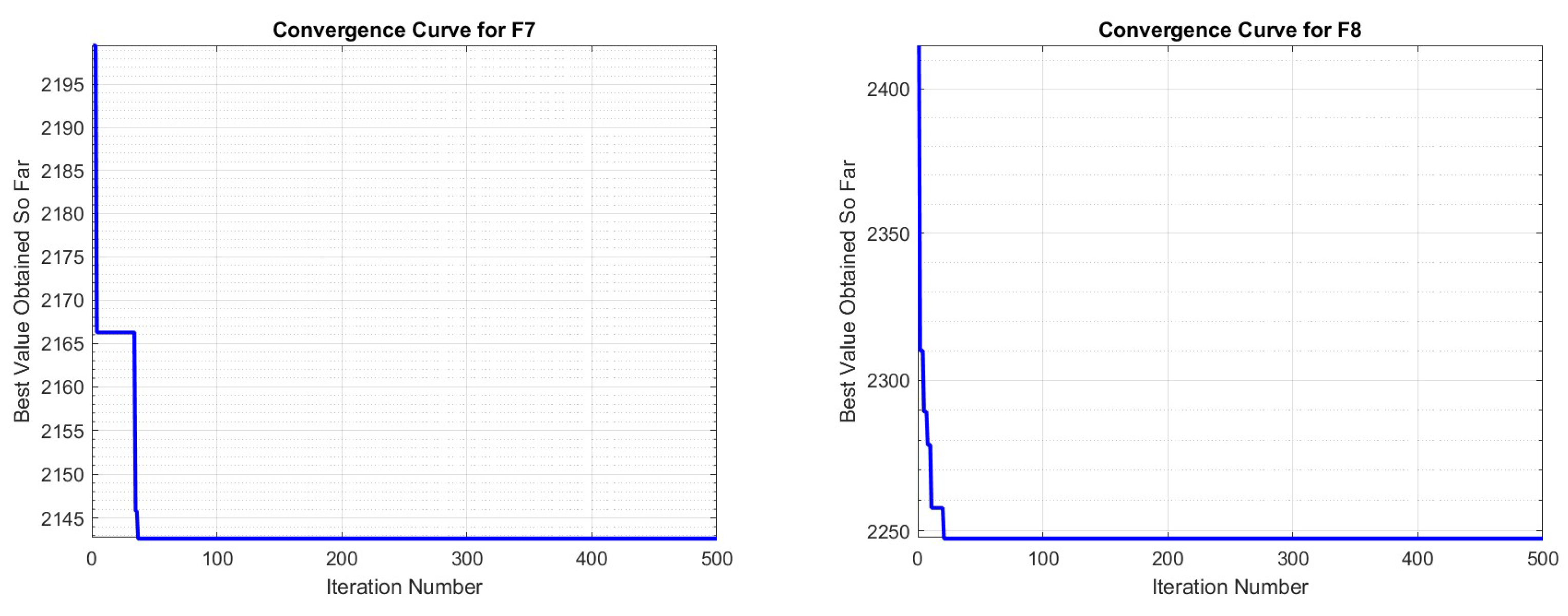
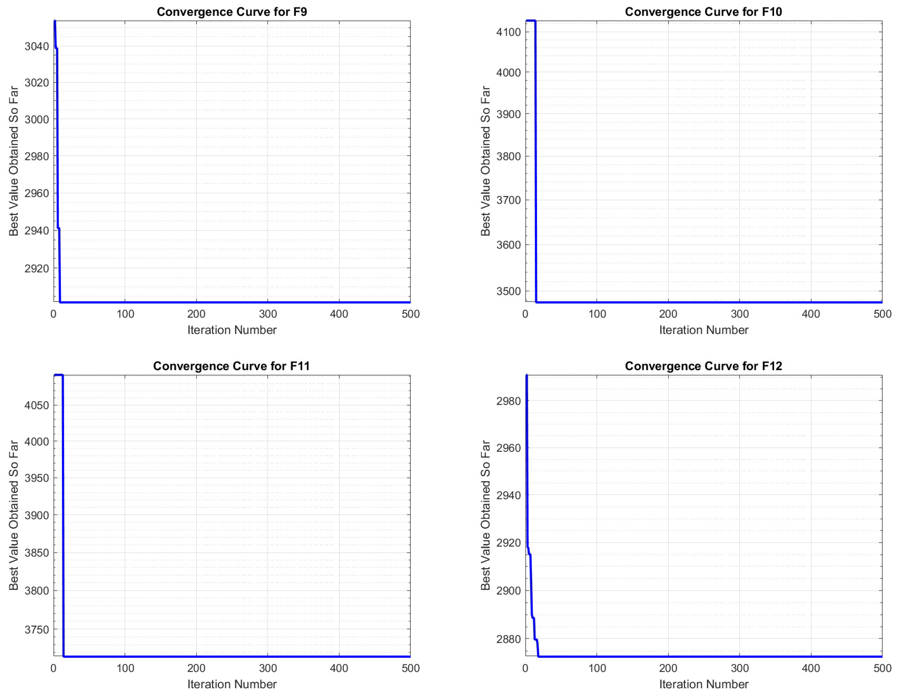
5.8.1. Convergence Curve Analysis
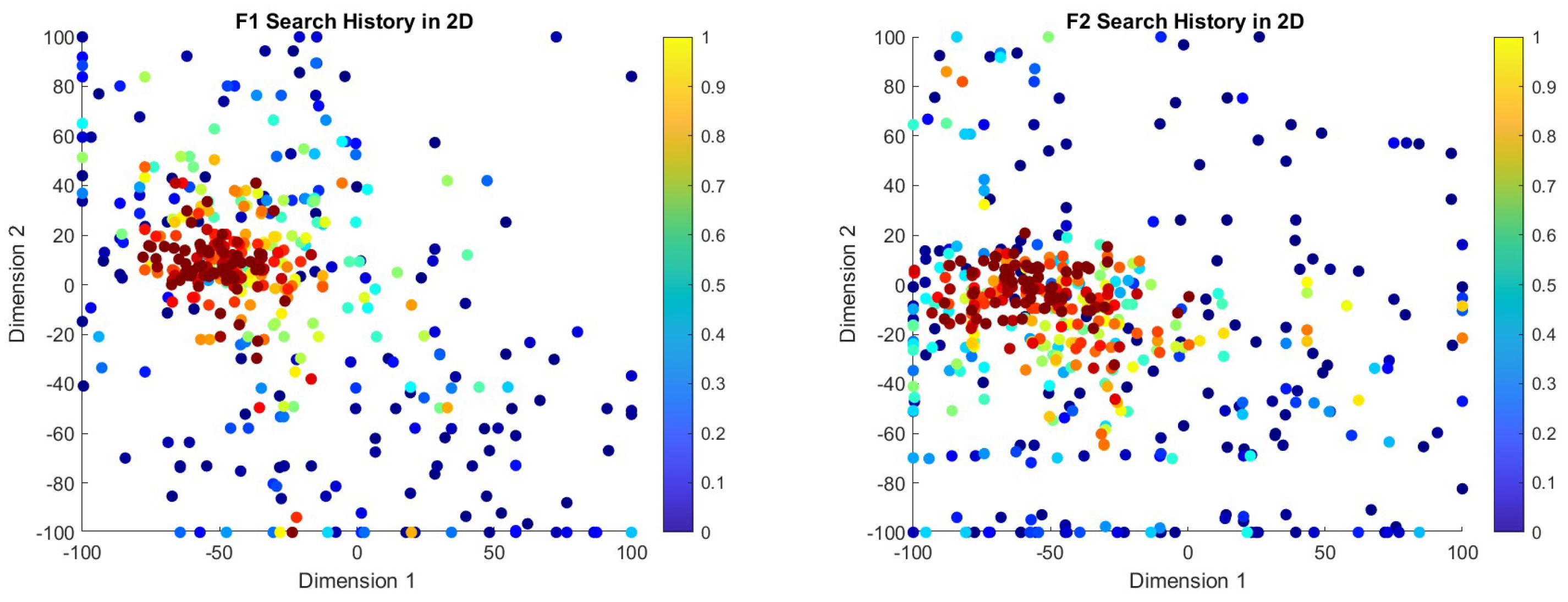
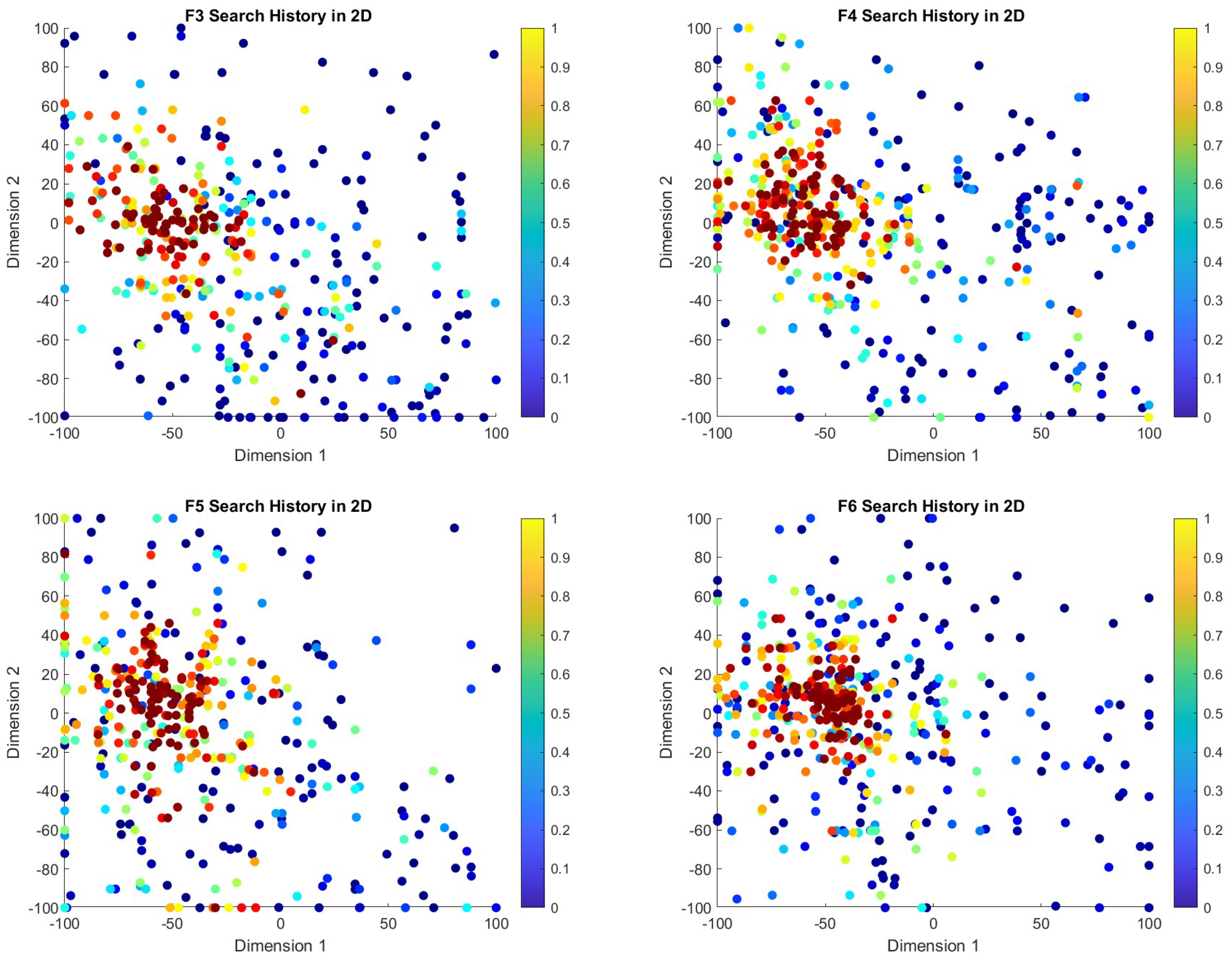
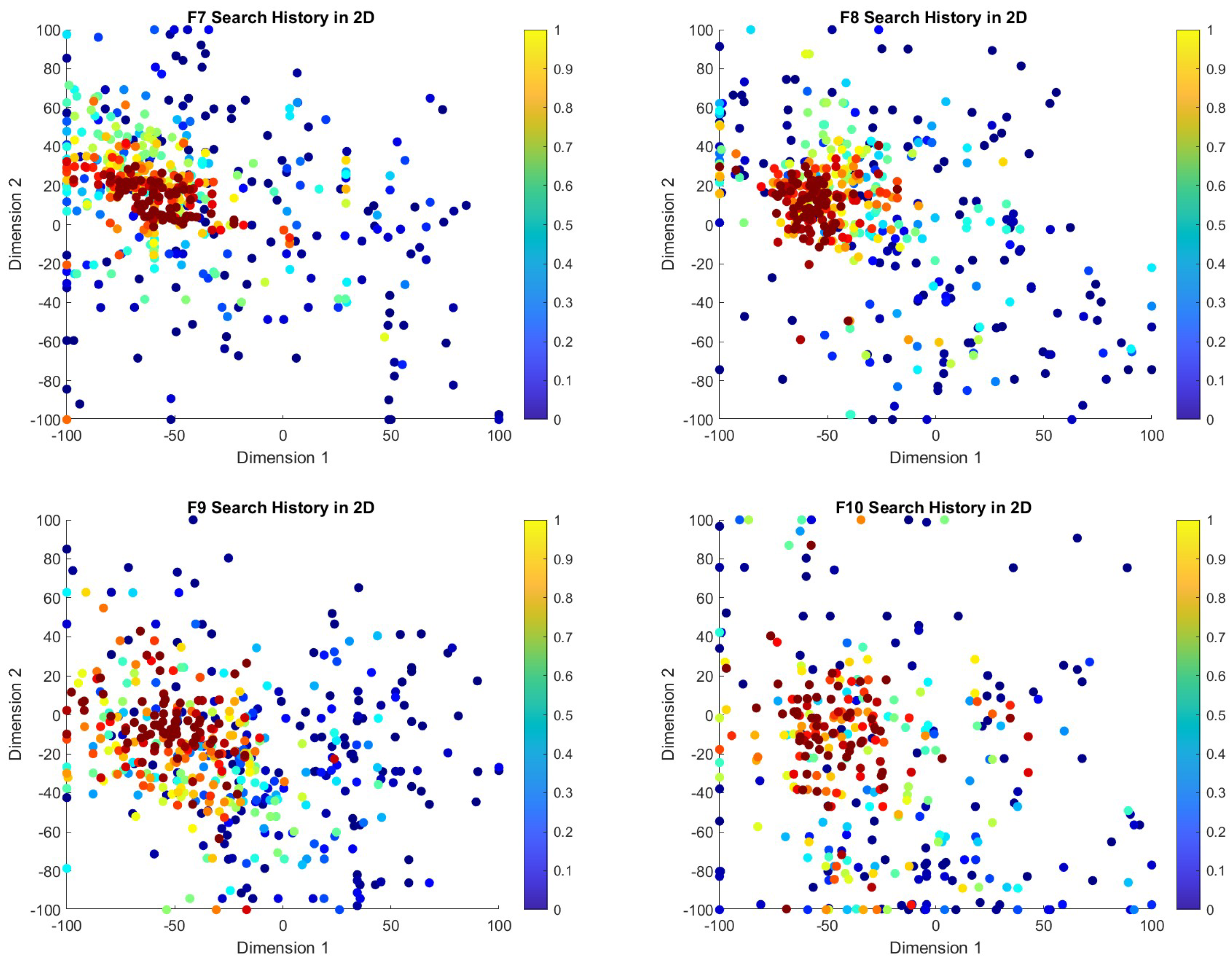
5.8.2. Search History Plot Analysis
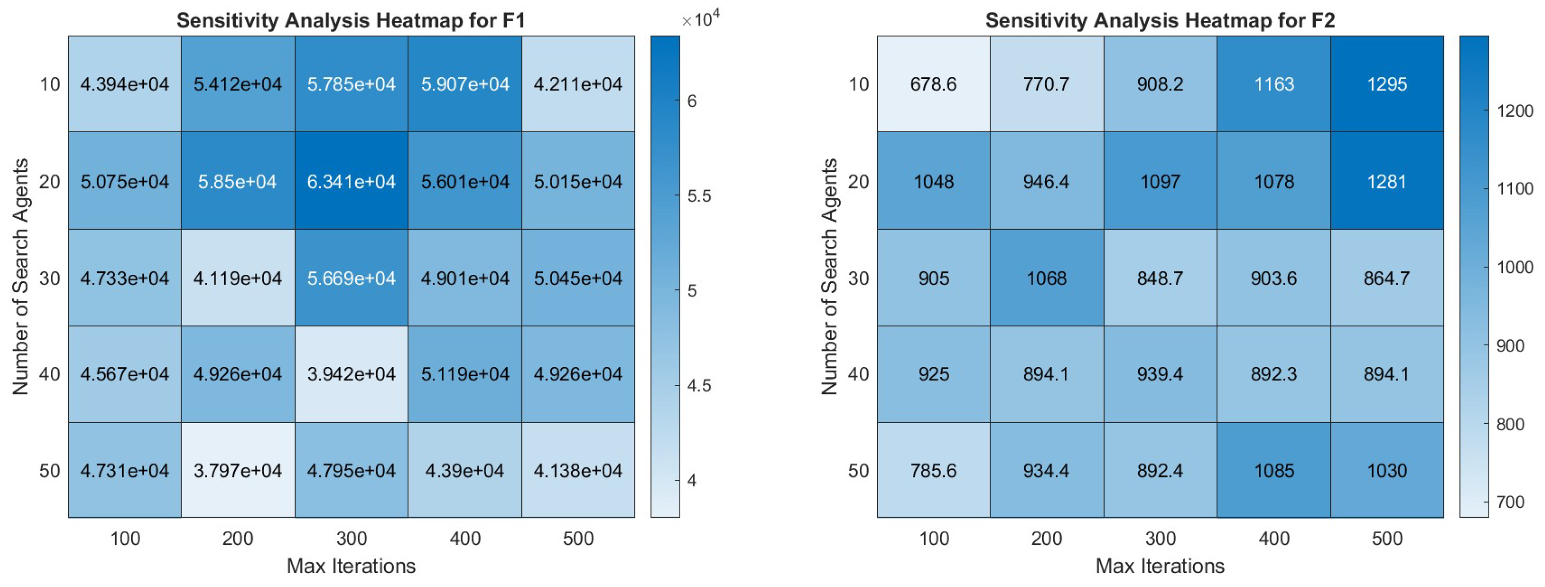
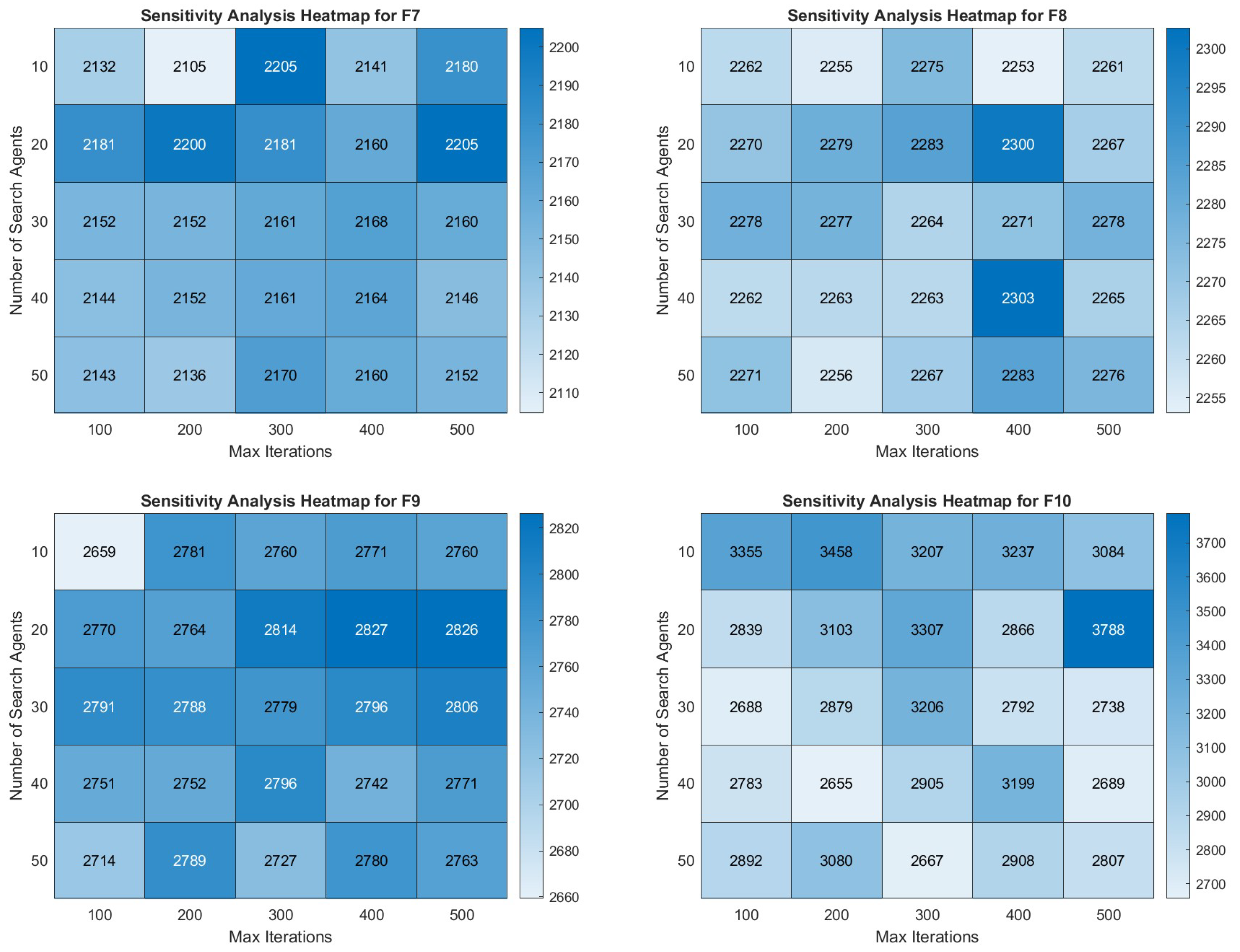
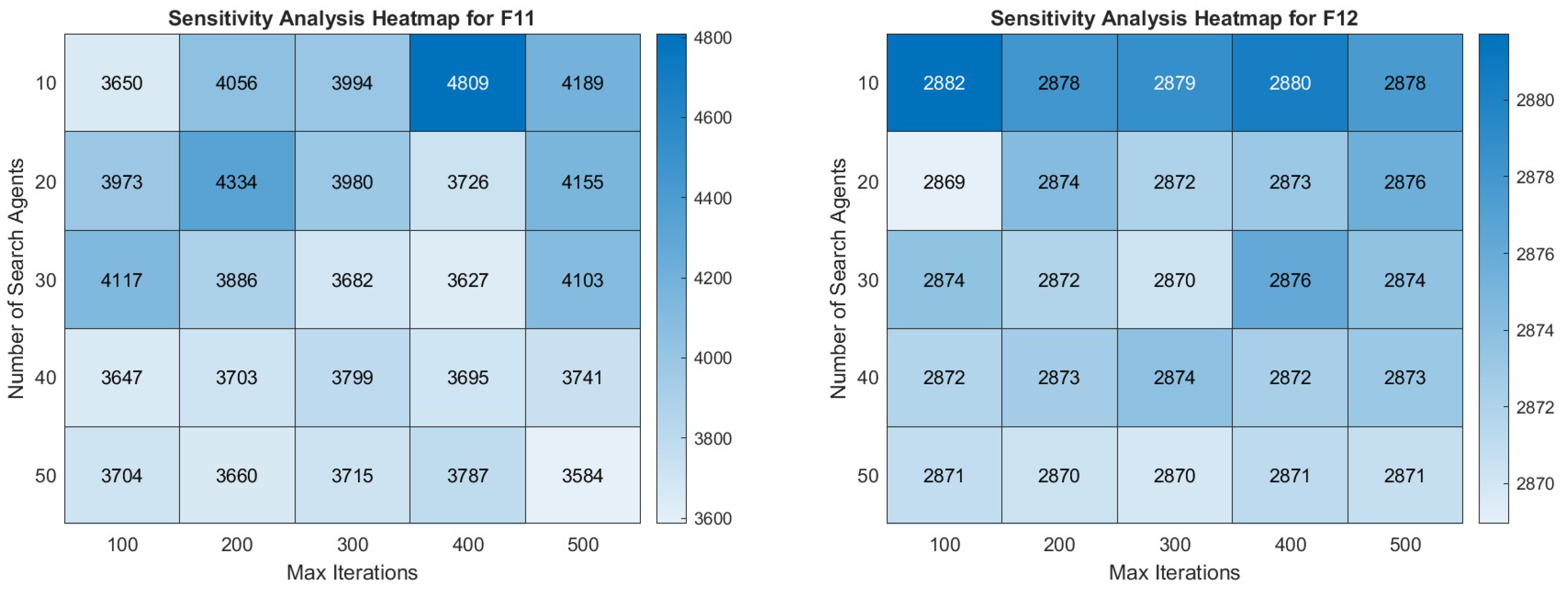
5.8.3. Sensitivity Analysis
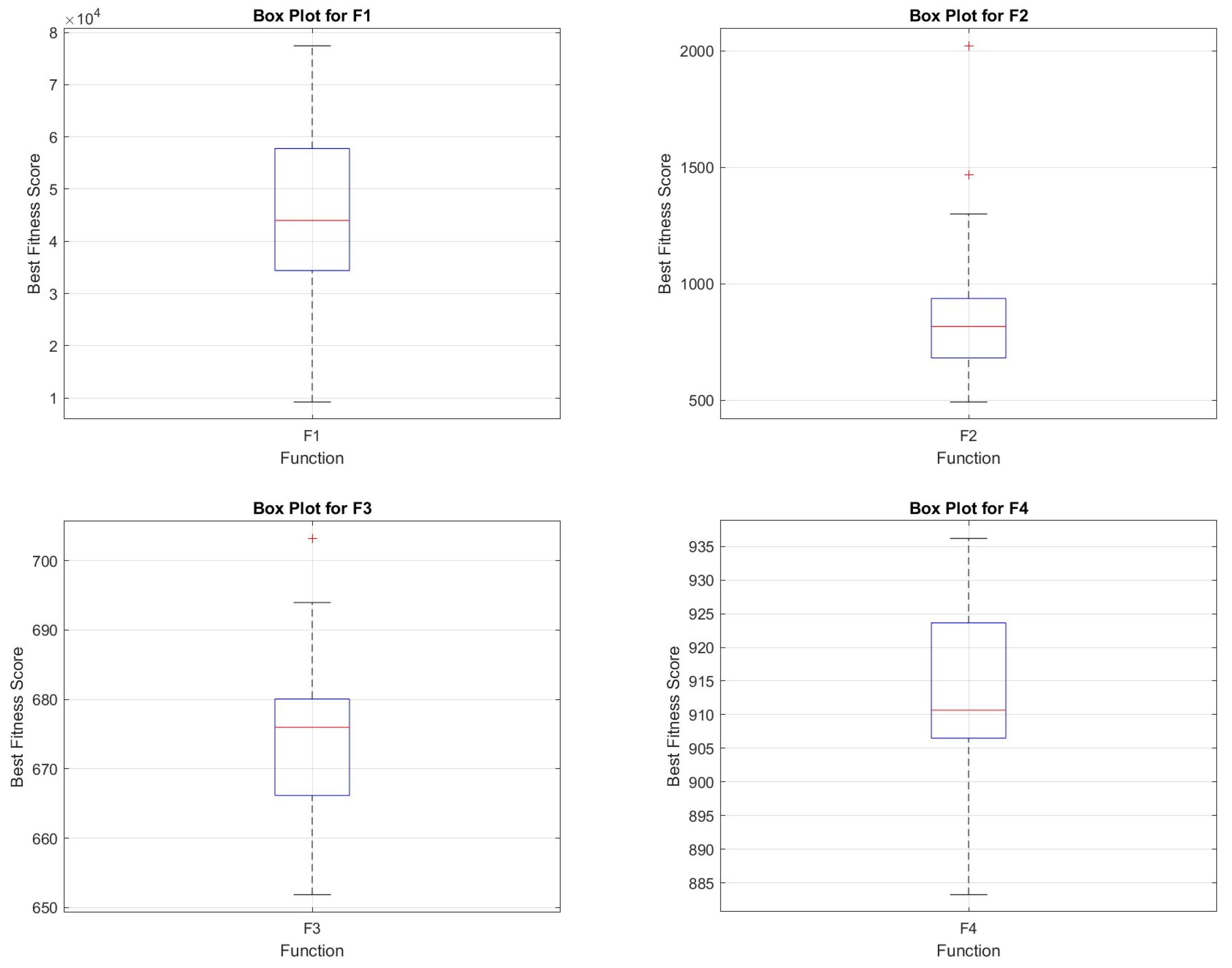
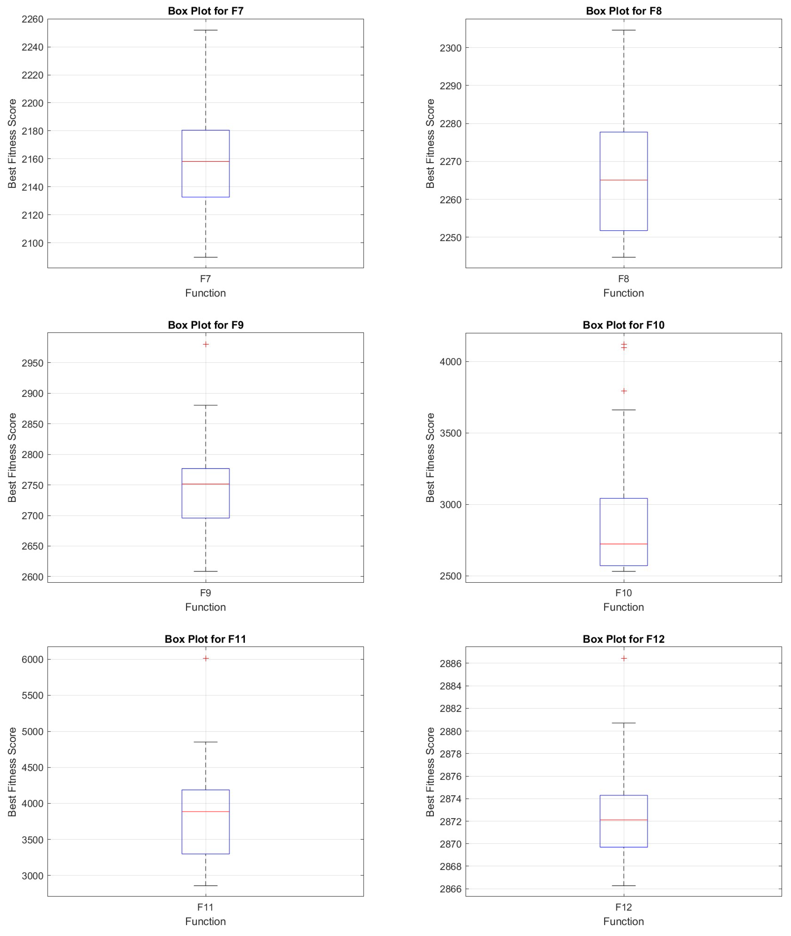
5.8.4. Box Plot Analysis
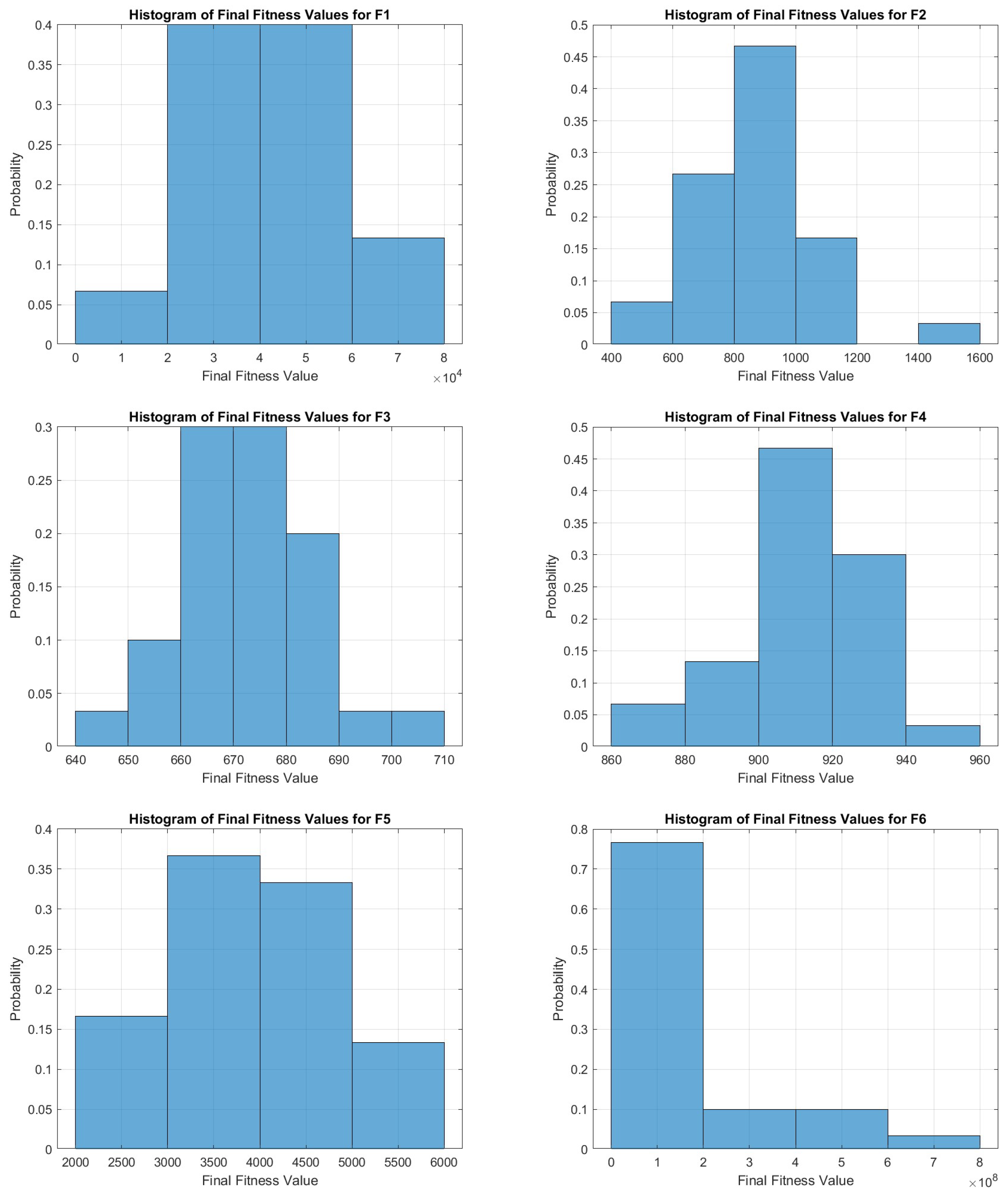
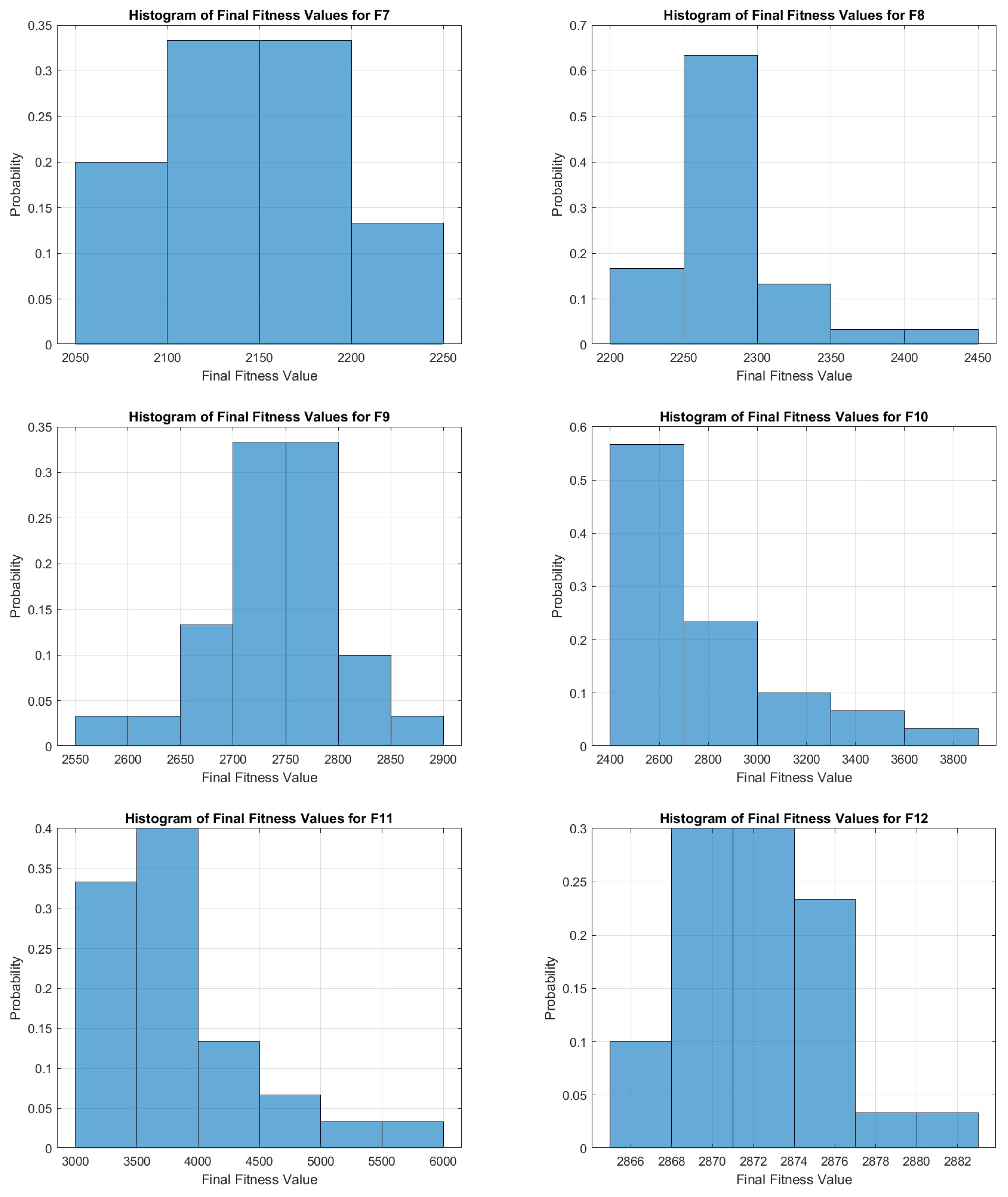
5.9. Histogram Analysis
6. Application of COASaD for Solving Engineering Design Problems
6.1. Welded Beam Design Problem
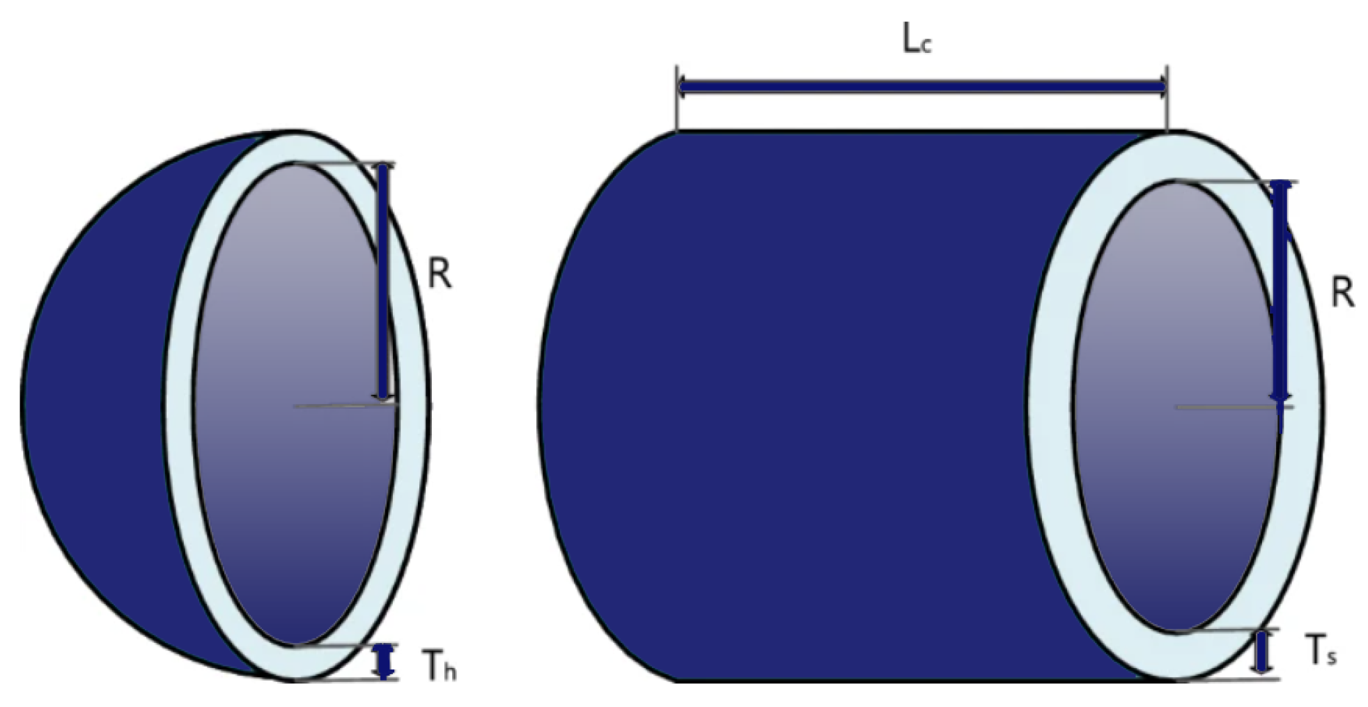
6.2. Pressure Vessel Design Problem
6.3. Spring Design Problem
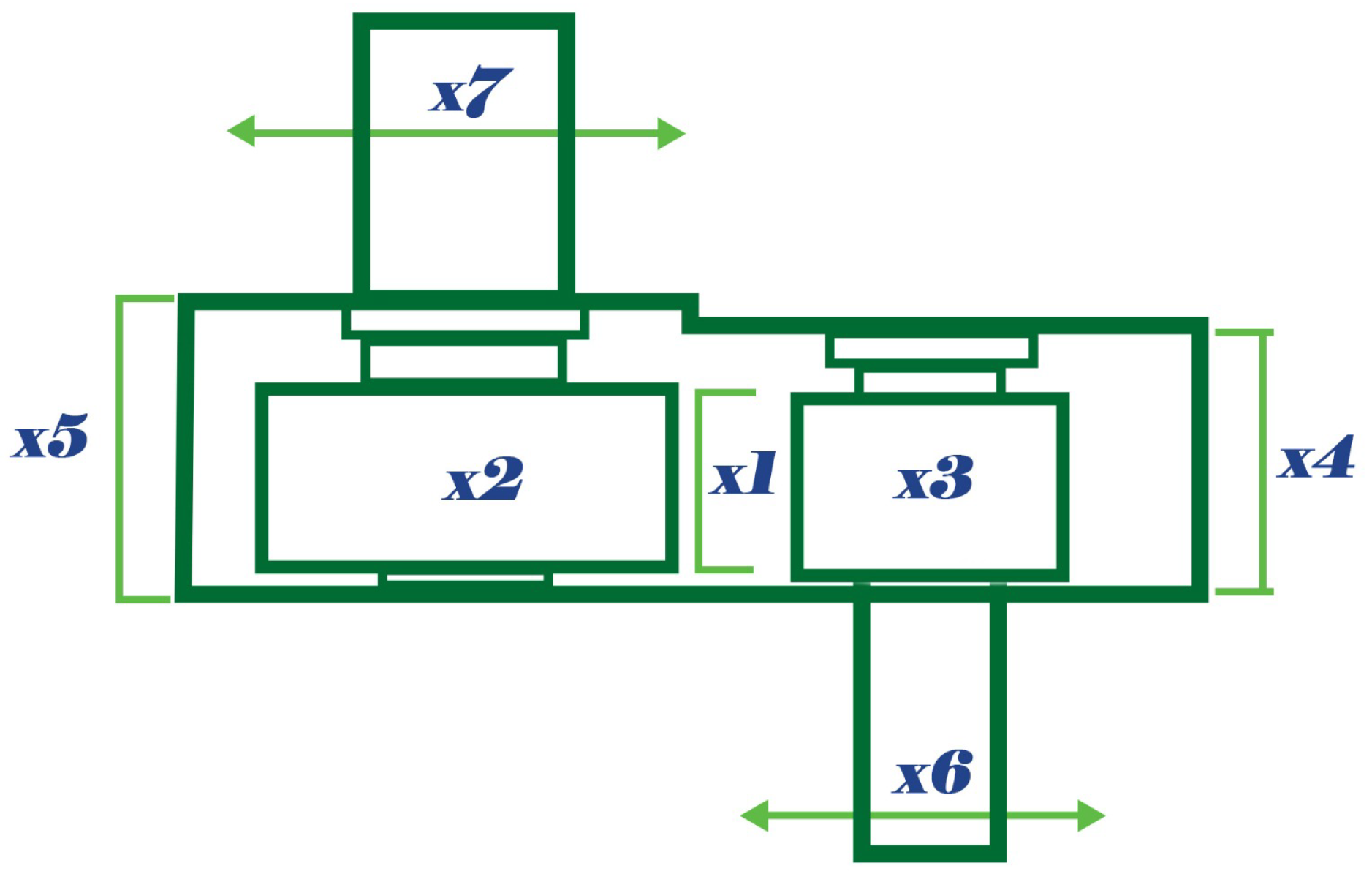
6.4. Speed Reducer Design Problem
6.5. Cantiliver Design Problem
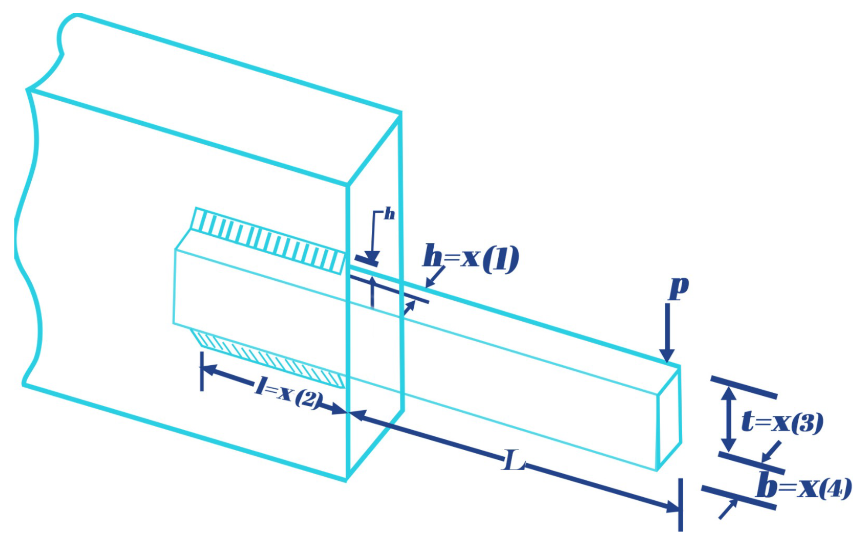
6.6. I-Beam Design Problem
6.7. Three-Bar Design Problem
7. Conclusions
Author Contributions
Funding
Data Availability Statement
Conflicts of Interest
References
- Abdel-Basset, M.; Abdel-Fatah, L.; Sangaiah, A.K. Metaheuristic algorithms: A comprehensive review. In Computational Intelligence for Multimedia Big Data on the Cloud with Engineering Applications; Academic Press: Cambridge, MA, USA, 2018; pp. 185–231. [Google Scholar]
- Kochenderfer, M.J.; Wheeler, T.A. Algorithms for Optimization; MIT Press: Cambridge, MA, USA, 2019. [Google Scholar]
- Diwekar, U.M. Introduction to Applied Optimization; Springer Nature: Berlin/Heidelberg, Germany, 2020; Volume 22. [Google Scholar]
- Blei, D.M.; Ng, A.Y.; Jordan, M.I. Latent dirichlet allocation. J. Mach. Learn. Res. 2003, 3, 993–1022. [Google Scholar]
- Fakhouri, H.N.; Alawadi, S.; Awaysheh, F.M.; Hamad, F. Novel hybrid success history intelligent optimizer with gaussian transformation: Application in CNN hyperparameter tuning. Clust. Comput. 2023, 27, 3717–3739. [Google Scholar] [CrossRef]
- Li, Q.; Tai, C.; Weinan, E. Stochastic modified equations and dynamics of stochastic gradient algorithms i: Mathematical foundations. J. Mach. Learn. Res. 2019, 20, 1474–1520. [Google Scholar]
- Gill, P.E.; Murray, W.; Wright, M.H. Practical Optimization; SIAM: Philadelphia, PA, USA, 2019. [Google Scholar]
- Yin, Z.Y.; Jin, Y.F.; Shen, J.S.; Hicher, P.Y. Optimization techniques for identifying soil parameters in geotechnical engineering: Comparative study and enhancement. Int. J. Numer. Anal. Methods Geomech. 2018, 42, 70–94. [Google Scholar] [CrossRef]
- Guo, K.; Yang, Z.; Yu, C.H.; Buehler, M.J. Artificial intelligence and machine learning in design of mechanical materials. Mater. Horizons 2021, 8, 1153–1172. [Google Scholar] [CrossRef] [PubMed]
- Fakhouri, S.N.; Hudaib, A.; Fakhouri, H.N. Enhanced optimizer algorithm and its application to software testing. J. Exp. Theor. Artif. Intell. 2020, 32, 885–907. [Google Scholar] [CrossRef]
- Shukri, S.E.; Al-Sayyed, R.; Hudaib, A.; Mirjalili, S. Enhanced multi-verse optimizer for task scheduling in cloud computing environments. Expert Syst. Appl. 2021, 168, 114230. [Google Scholar] [CrossRef]
- Hudaib, A.A.; Fakhouri, H.N. Supernova optimizer: A novel natural inspired meta-heuristic. Mod. Appl. Sci. 2018, 12, 32–50. [Google Scholar] [CrossRef]
- Fakhouri, H.N.; Alawadi, S.; Awaysheh, F.M.; Hani, I.B.; Alkhalaileh, M.; Hamad, F. A comprehensive study on the role of machine learning in 5G security: Challenges, technologies, and solutions. Electronics 2023, 12, 4604. [Google Scholar] [CrossRef]
- Zhan, Z.H.; Shi, L.; Tan, K.C.; Zhang, J. A survey on evolutionary computation for complex continuous optimization. Artif. Intell. Rev. 2022, 55, 59–110. [Google Scholar] [CrossRef]
- Ahvanooey, M.T.; Li, Q.; Wu, M.; Wang, S. A survey of genetic programming and its applications. KSII Trans. Internet Inf. Syst. (TIIS) 2019, 13, 1765–1794. [Google Scholar]
- Žilinskas, A.; Calvin, J. Bi-objective decision making in global optimization based on statistical models. J. Glob. Optim. 2019, 74, 599–609. [Google Scholar] [CrossRef]
- Fakhouri, H.N.; Hudaib, A.; Sleit, A. Hybrid particle swarm optimization with sine cosine algorithm and nelder–mead simplex for solving engineering design problems. Arab. J. Sci. Eng. 2020, 45, 3091–3109. [Google Scholar] [CrossRef]
- Lan, G. First-Order and Stochastic Optimization Methods for Machine Learning; Springer: Berlin/Heidelberg, Germany, 2020; Volume 1. [Google Scholar]
- Diakonikolas, I.; Kamath, G.; Kane, D.; Li, J.; Steinhardt, J.; Stewart, A. Sever: A robust meta-algorithm for stochastic optimization. In Proceedings of the International Conference on Machine Learning, Long Beach, CA, USA, 9–15 June 2019; pp. 1596–1606. [Google Scholar]
- Fakhouri, H.N.; Hudaib, A.; Sleit, A. Multivector particle swarm optimization algorithm. Soft Comput. 2020, 24, 11695–11713. [Google Scholar] [CrossRef]
- Erol, O.K.; Eksin, I. A new optimization method: Big bang–big crunch. Adv. Eng. Softw. 2006, 37, 106–111. [Google Scholar] [CrossRef]
- Powell, W.B. A unified framework for stochastic optimization. Eur. J. Oper. Res. 2019, 275, 795–821. [Google Scholar] [CrossRef]
- Bitar, R.; Wootters, M.; El Rouayheb, S. Stochastic gradient coding for straggler mitigation in distributed learning. IEEE J. Sel. Areas Inf. Theory 2020, 1, 277–291. [Google Scholar] [CrossRef]
- Mathew, T.V. Genetic Algorithm. 2012. Available online: https://datajobs.com/data-science-repo/Genetic-Algorithm-Guide-[Tom-Mathew].pdf (accessed on 9 June 2024).
- Zedadra, O.; Guerrieri, A.; Jouandeau, N.; Spezzano, G.; Seridi, H.; Fortino, G. Swarm intelligence-based algorithms within IoT-based systems: A review. J. Parallel Distrib. Comput. 2018, 122, 173–187. [Google Scholar] [CrossRef]
- Dorigo, M.; Stützle, T. Ant Colony Optimization: Overview and Recent Advances; Springer: Berlin/Heidelberg, Germany, 2019. [Google Scholar]
- Fakhouri, H.N.; Awaysheh, F.M.; Alawadi, S.; Alkhalaileh, M.; Hamad, F. Four vector intelligent metaheuristic for data optimization. Computing 2024, 106, 2321–2359. [Google Scholar] [CrossRef]
- Yang, X.S. Nature-Inspired Optimization Algorithms; Academic Press: Cambridge, MA, USA, 2020. [Google Scholar]
- Deng, W.; Xu, J.; Gao, X.Z.; Zhao, H. An enhanced MSIQDE algorithm with novel multiple strategies for global optimization problems. IEEE Trans. Syst. Man Cybern. Syst. 2020, 52, 1578–1587. [Google Scholar] [CrossRef]
- Seyyedabbasi, A. WOASCALF: A new hybrid whale optimization algorithm based on sine cosine algorithm and levy flight to solve global optimization problems. Adv. Eng. Softw. 2022, 173, 103272. [Google Scholar] [CrossRef]
- Ashraf, A.; Almazroi, A.A.; Bangyal, W.H.; Alqarni, M.A. Particle Swarm Optimization with New Initializing Technique to Solve Global Optimization Problems. Intell. Autom. Soft Comput. 2022, 31, 191. [Google Scholar] [CrossRef]
- Che, Y.; He, D. A hybrid whale optimization with seagull algorithm for global optimization problems. Math. Probl. Eng. 2021, 2021, 6639671. [Google Scholar] [CrossRef]
- Braik, M.; Al-Zoubi, H.; Ryalat, M.; Sheta, A.; Alzubi, O. Memory based hybrid crow search algorithm for solving numerical and constrained global optimization problems. Artif. Intell. Rev. 2023, 56, 27–99. [Google Scholar] [CrossRef]
- Wang, Z.; Luo, Q.; Zhou, Y. Hybrid metaheuristic algorithm using butterfly and flower pollination base on mutualism mechanism for global optimization problems. Eng. Comput. 2021, 37, 3665–3698. [Google Scholar] [CrossRef]
- Jia, H.; Zhou, X.; Zhang, J.; Abualigah, L.; Yildiz, A.R.; Hussien, A.G. Modified crayfish optimization algorithm for solving multiple engineering application problems. Artif. Intell. Rev. 2024, 57, 127. [Google Scholar] [CrossRef]
- Daulat, H.; Varma, T.; Chauhan, K. Augmenting the Crayfish Optimization with Gaussian Distribution Parameter for Improved Optimization Efficiency. In Proceedings of the 2024 International Conference on Cognitive Robotics and Intelligent Systems (ICC-ROBINS), Tamil Nadu, India, 17–19 April 2024; pp. 462–470. [Google Scholar]
- Jia, H.; Rao, H.; Wen, C.; Mirjalili, S. Crayfish optimization algorithm. Artif. Intell. Rev. 2023, 56, 1919–1979. [Google Scholar] [CrossRef]
- Qin, A.K.; Suganthan, P.N. Self-adaptive differential evolution algorithm for numerical optimization. In Proceedings of the 2005 IEEE Congress on Evolutionary Computation, Scotland, UK, 2–5 September 2005; Volume 2, pp. 1785–1791. [Google Scholar]
- Eltaeib, T.; Mahmood, A. Differential evolution: A survey and analysis. Appl. Sci. 2018, 8, 1945. [Google Scholar] [CrossRef]
- Pepelyshev, A.; Zhigljavsky, A.; Žilinskas, A. Performance of global random search algorithms for large dimensions. J. Glob. Optim. 2018, 71, 57–71. [Google Scholar]
- Ye, P.; Pan, G. Selecting the best quantity and variety of surrogates for an ensemble model. Mathematics 2020, 8, 1721. [Google Scholar] [CrossRef]


| Parameter Type | Assigned Value |
|---|---|
| Size of Population | 30 individuals |
| Evaluation Limit | 1000 iterations |
| Problem Dimensions (D) | 10 |
| Boundary of Search | |
| Incorporation of Rotation | Applied where specified |
| Application of Shift | Applied where specified |
| Algorithm | Parameter |
|---|---|
| MFO | a linearly decreases from −1 to −2 |
| GWO | Convergence constant a = [2, 0] |
| PSO | , , , |
| MVO | Modular modality = 0.01, Power exponent = v, Switch probability = 0.8 |
| AOA | , Mu = 0.499 |
| MVO | , |
| SHO | U = 0.05, V = 0.05, L = 0.05 |
| SCA | , , , |
| Function | Statistics | COASaDE | GWO | PSO | MFO | MVO | SHIO | OHO | AOA | FOX | FVIM | SCA |
|---|---|---|---|---|---|---|---|---|---|---|---|---|
| F1 | Mean | 3.00E+02 | 8.90E+02 | 1.58E+04 | 1.09E+04 | 8.80E+03 | 6.68E+03 | 1.20E+04 | 6.32E+03 | 1.17E+03 | 7.44E+02 | 1.39E+03 |
| Std | 1.42E-04 | 1.05E+03 | 5.10E+03 | 9.50E+03 | 4.51E+03 | 3.42E+03 | 2.05E+03 | 2.54E+03 | 4.53E+02 | 6.02E+02 | 1.41E+03 | |
| SEM | 6.34E-05 | 4.70E+02 | 2.28E+03 | 4.25E+03 | 2.02E+03 | 1.53E+03 | 9.18E+02 | 1.14E+03 | 2.03E+02 | 2.69E+02 | 6.31E+02 | |
| Rank | 1 | 3 | 11 | 9 | 8 | 7 | 10 | 6 | 4 | 2 | 5 | |
| F2 | Mean | 4.05E+02 | 4.26E+02 | 4.14E+02 | 4.10E+02 | 1.71E+03 | 4.49E+02 | 3.03E+03 | 8.06E+02 | 4.55E+02 | 4.42E+02 | 4.61E+02 |
| Std | 1.94E+00 | 3.07E+01 | 1.38E+01 | 5.29E+00 | 5.52E+02 | 3.73E+01 | 1.41E+03 | 1.01E+02 | 1.24E+01 | 2.28E+01 | 3.46E+01 | |
| SEM | 8.68E-01 | 1.37E+01 | 6.19E+00 | 2.36E+00 | 2.47E+02 | 1.67E+01 | 6.29E+02 | 4.53E+01 | 5.54E+00 | 1.02E+01 | 1.55E+01 | |
| Rank | 1 | 4 | 3 | 2 | 10 | 6 | 11 | 9 | 7 | 5 | 8 | |
| F3 | Mean | 6.00E+02 | 6.00E+02 | 6.33E+02 | 6.02E+02 | 6.42E+02 | 6.05E+02 | 6.55E+02 | 6.36E+02 | 6.14E+02 | 6.05E+02 | 6.15E+02 |
| Std | 0.00E+00 | 3.33E-01 | 1.13E+01 | 2.55E+00 | 5.20E+00 | 5.29E+00 | 6.88E+00 | 6.04E+00 | 2.75E+00 | 3.24E+00 | 8.51E+00 | |
| SEM | 0.00E+00 | 1.49E-01 | 5.06E+00 | 1.14E+00 | 2.33E+00 | 2.36E+00 | 3.08E+00 | 2.70E+00 | 1.23E+00 | 1.45E+00 | 3.80E+00 | |
| Rank | 1 | 2 | 8 | 3 | 10 | 5 | 11 | 9 | 6 | 4 | 7 | |
| F4 | Mean | 8.27E+02 | 8.15E+02 | 8.35E+02 | 8.35E+02 | 8.50E+02 | 8.12E+02 | 8.48E+02 | 8.30E+02 | 8.37E+02 | 8.28E+02 | 8.28E+02 |
| Std | 3.29E+00 | 5.10E+00 | 1.26E+01 | 3.27E+00 | 5.63E+00 | 2.85E+00 | 2.96E+00 | 3.61E+00 | 7.36E+00 | 6.65E+00 | 8.70E+00 | |
| SEM | 1.47E+00 | 2.28E+00 | 5.65E+00 | 1.46E+00 | 2.52E+00 | 1.28E+00 | 1.32E+00 | 1.62E+00 | 3.29E+00 | 2.97E+00 | 3.89E+00 | |
| Rank | 3 | 2 | 7 | 8 | 11 | 1 | 10 | 6 | 9 | 5 | 4 | |
| F5 | Mean | 9.00E+02 | 9.01E+02 | 1.32E+03 | 9.77E+02 | 1.33E+03 | 9.92E+02 | 1.55E+03 | 1.31E+03 | 9.99E+02 | 9.52E+02 | 1.05E+03 |
| Std | 0.00E+00 | 8.21E-01 | 2.83E+02 | 1.31E+02 | 8.38E+01 | 1.01E+02 | 4.61E+01 | 1.32E+02 | 1.83E+01 | 3.92E+01 | 1.26E+02 | |
| SEM | 0.00E+00 | 3.67E-01 | 1.27E+02 | 5.85E+01 | 3.75E+01 | 4.51E+01 | 2.06E+01 | 5.90E+01 | 8.18E+00 | 1.76E+01 | 5.61E+01 | |
| Rank | 1 | 2 | 9 | 4 | 10 | 5 | 11 | 8 | 6 | 3 | 7 | |
| F6 | Mean | 1.80E+03 | 5.71E+03 | 2.74E+03 | 5.72E+03 | 4.59E+07 | 2.99E+03 | 1.26E+09 | 3.68E+03 | 1.65E+06 | 1.01E+04 | 4.56E+03 |
| Std | 5.26E-01 | 3.35E+03 | 1.38E+03 | 2.53E+03 | 7.73E+07 | 1.06E+03 | 9.46E+08 | 8.62E+02 | 1.18E+06 | 2.55E+03 | 1.76E+03 | |
| SEM | 2.35E-01 | 1.50E+03 | 6.18E+02 | 1.13E+03 | 3.46E+07 | 4.72E+02 | 4.23E+08 | 3.86E+02 | 5.27E+05 | 1.14E+03 | 7.89E+02 | |
| Rank | 1 | 6 | 2 | 7 | 10 | 3 | 11 | 4 | 9 | 8 | 5 | |
| F7 | Mean | 2.00E+03 | 2.03E+03 | 2.06E+03 | 2.03E+03 | 2.09E+03 | 2.05E+03 | 2.12E+03 | 2.11E+03 | 2.05E+03 | 2.05E+03 | 2.03E+03 |
| Std | 9.39E+00 | 2.35E+01 | 2.10E+01 | 1.65E+01 | 1.75E+01 | 1.88E+01 | 1.06E+01 | 1.99E+01 | 5.12E+00 | 1.79E+01 | 1.59E+01 | |
| SEM | 4.20E+00 | 1.05E+01 | 9.40E+00 | 7.37E+00 | 7.81E+00 | 8.40E+00 | 4.76E+00 | 8.88E+00 | 2.29E+00 | 8.00E+00 | 7.12E+00 | |
| Rank | 1 | 2 | 8 | 3 | 9 | 6 | 11 | 10 | 7 | 5 | 4 | |
| F8 | Mean | 2.20E+03 | 2.22E+03 | 2.24E+03 | 2.22E+03 | 2.33E+03 | 2.23E+03 | 2.37E+03 | 2.29E+03 | 2.23E+03 | 2.23E+03 | 2.22E+03 |
| Std | 1.05E+00 | 2.24E+00 | 1.80E+01 | 1.96E+00 | 8.44E+01 | 5.01E+00 | 6.65E+01 | 1.03E+02 | 2.94E+00 | 6.57E-01 | 2.28E+00 | |
| SEM | 4.71E-01 | 1.00E+00 | 8.07E+00 | 8.75E-01 | 3.77E+01 | 2.24E+00 | 2.97E+01 | 4.61E+01 | 1.31E+00 | 2.94E-01 | 1.02E+00 | |
| Rank | 1 | 2 | 8 | 3 | 10 | 6 | 11 | 9 | 7 | 5 | 4 | |
| F9 | Mean | 2.53E+03 | 2.54E+03 | 2.55E+03 | 2.53E+03 | 2.79E+03 | 2.56E+03 | 2.82E+03 | 2.70E+03 | 2.57E+03 | 2.58E+03 | 2.57E+03 |
| Std | 0.00E+00 | 1.86E+01 | 2.88E+01 | 2.49E-01 | 8.91E+01 | 3.38E+01 | 3.82E+01 | 2.23E+01 | 2.04E+01 | 3.20E+01 | 2.03E+01 | |
| SEM | 0.00E+00 | 8.31E+00 | 1.29E+01 | 1.11E-01 | 3.98E+01 | 1.51E+01 | 1.71E+01 | 9.96E+00 | 9.13E+00 | 1.43E+01 | 9.06E+00 | |
| Rank | 1 | 3 | 4 | 2 | 10 | 5 | 11 | 9 | 6 | 8 | 7 | |
| F10 | Mean | 2.50E+03 | 2.57E+03 | 2.66E+03 | 2.50E+03 | 2.50E+03 | 2.53E+03 | 3.14E+03 | 2.74E+03 | 2.50E+03 | 2.55E+03 | 2.58E+03 |
| Std | 5.96E-02 | 6.05E+01 | 1.99E+02 | 1.24E+00 | 1.08E+00 | 5.54E+01 | 4.27E+02 | 2.00E+02 | 4.05E-01 | 6.42E+01 | 6.89E+01 | |
| SEM | 2.67E-02 | 2.71E+01 | 8.89E+01 | 5.55E-01 | 4.81E-01 | 2.48E+01 | 1.91E+02 | 8.95E+01 | 1.81E-01 | 2.87E+01 | 3.08E+01 | |
| Rank | 1 | 7 | 9 | 2 | 4 | 5 | 11 | 10 | 3 | 6 | 8 | |
| F11 | Mean | 2.60E+03 | 2.87E+03 | 2.84E+03 | 2.70E+03 | 2.99E+03 | 2.83E+03 | 3.69E+03 | 3.20E+03 | 2.77E+03 | 2.94E+03 | 2.72E+03 |
| Std | 3.94E-13 | 2.12E+02 | 1.20E+02 | 9.31E+01 | 1.30E+02 | 2.64E+02 | 7.01E+02 | 3.10E+02 | 4.19E+00 | 2.37E+02 | 5.71E+01 | |
| SEM | 1.76E-13 | 9.46E+01 | 5.37E+01 | 4.16E+01 | 5.81E+01 | 1.18E+02 | 3.14E+02 | 1.38E+02 | 1.87E+00 | 1.06E+02 | 2.56E+01 | |
| Rank | 1 | 7 | 6 | 2 | 9 | 5 | 11 | 10 | 4 | 8 | 3 | |
| F12 | Mean | 2.86E+03 | 2.87E+03 | 2.89E+03 | 2.86E+03 | 2.90E+03 | 2.88E+03 | 3.09E+03 | 2.99E+03 | 2.87E+03 | 2.87E+03 | 2.89E+03 |
| Std | 7.50E-01 | 2.48E+00 | 3.03E+01 | 7.52E-01 | 2.25E+01 | 1.43E+01 | 4.32E+01 | 3.01E+01 | 1.73E+00 | 3.40E+00 | 2.20E+01 | |
| SEM | 3.35E-01 | 1.11E+00 | 1.36E+01 | 3.36E-01 | 1.01E+01 | 6.37E+00 | 1.93E+01 | 1.34E+01 | 7.72E-01 | 1.52E+00 | 9.85E+00 | |
| Rank | 1 | 3 | 8 | 2 | 9 | 6 | 11 | 10 | 5 | 4 | 7 |
| Function | Statistics | COASaDE | COA | LDE | BBDE | ODE | JADE | DEEM | SADE | CMAES |
|---|---|---|---|---|---|---|---|---|---|---|
| F1 | Mean | 3.00E+02 | 3.01E+02 | 3.18E+02 | 8.25E+02 | 3.00E+02 | 3.64E+02 | 3.01E+02 | 7.65E+02 | 2.28E+04 |
| Std | 1.42E-04 | 6.39E-01 | 1.09E+01 | 6.10E+02 | 1.38E-03 | 8.27E+01 | 0.00E+00 | 2.53E+02 | 1.08E+04 | |
| SEM | 6.34E-05 | 2.86E-01 | 4.88E+00 | 2.73E+02 | 6.17E-04 | 3.70E+01 | 0.00E+00 | 1.13E+02 | 4.81E+03 | |
| Rank | 1 | 4 | 5 | 8 | 2 | 6 | 3 | 7 | 9 | |
| F2 | Mean | 4.05E+02 | 4.06E+02 | 4.08E+02 | 4.07E+02 | 4.08E+02 | 4.07E+02 | 4.06E+02 | 4.08E+02 | 5.80E+02 |
| Std | 1.94E+00 | 3.50E+00 | 1.76E+00 | 1.64E+00 | 1.87E+00 | 2.64E+00 | 4.05E+00 | 7.99E-01 | 6.89E+01 | |
| SEM | 8.68E-01 | 1.57E+00 | 7.87E-01 | 7.34E-01 | 8.34E-01 | 1.18E+00 | 1.81E+00 | 3.57E-01 | 3.08E+01 | |
| Rank | 1 | 2 | 6 | 5 | 7 | 4 | 3 | 8 | 9 | |
| F3 | Mean | 6.00E+02 | 6.07E+02 | 6.00E+02 | 6.00E+02 | 6.00E+02 | 6.00E+02 | 6.00E+02 | 6.00E+02 | 6.28E+02 |
| Std | 0.00E+00 | 1.35E+01 | 3.16E-02 | 8.04E-14 | 0.00E+00 | 7.85E-07 | 5.32E-02 | 0.00E+00 | 2.98E+01 | |
| SEM | 0.00E+00 | 6.03E+00 | 1.41E-02 | 3.60E-14 | 0.00E+00 | 3.51E-07 | 2.38E-02 | 0.00E+00 | 1.33E+01 | |
| Rank | 1 | 8 | 7 | 1 | 1 | 5 | 6 | 1 | 9 | |
| F4 | Mean | 8.27E+02 | 8.33E+02 | 8.30E+02 | 8.12E+02 | 8.30E+02 | 8.06E+02 | 8.11E+02 | 8.28E+02 | 8.27E+02 |
| Std | 3.29E+00 | 4.45E-01 | 3.85E+00 | 5.23E+00 | 1.74E+00 | 8.22E-01 | 7.22E+00 | 5.32E+00 | 1.04E+01 | |
| SEM | 1.47E+00 | 1.99E-01 | 1.72E+00 | 2.34E+00 | 7.80E-01 | 3.68E-01 | 3.23E+00 | 2.38E+00 | 4.65E+00 | |
| Rank | 4 | 9 | 8 | 3 | 7 | 1 | 2 | 6 | 5 | |
| F5 | Mean | 900 | 902.4721 | 900.2119 | 900.0179 | 900 | 900.0001 | 900.1088 | 900.0001 | 900 |
| Std | 0 | 4.641643 | 0.046755 | 0.040038 | 0 | 7.37E-05 | 0.243218 | 0.000172 | 0 | |
| SEM | 0 | 2.075806 | 0.02091 | 0.017906 | 0 | 3.3E-05 | 0.10877 | 7.68E-05 | 0 | |
| Rank | 1 | 9 | 8 | 6 | 1 | 4 | 7 | 5 | 1 | |
| F6 | Mean | 1.80E+03 | 3.64E+03 | 5.98E+03 | 2.77E+03 | 1.80E+03 | 1.85E+03 | 1.81E+03 | 1.84E+03 | 7.61E+07 |
| Std | 5.26E-01 | 2.56E+03 | 2.80E+03 | 1.08E+03 | 4.98E-01 | 2.79E+01 | 5.82E+00 | 1.47E+01 | 1.10E+08 | |
| SEM | 2.35E-01 | 1.14E+03 | 1.25E+03 | 4.83E+02 | 2.23E-01 | 1.25E+01 | 2.60E+00 | 6.57E+00 | 4.92E+07 | |
| Rank | 1 | 7 | 8 | 6 | 2 | 5 | 3 | 4 | 9 | |
| F7 | Mean | 2.00E+03 | 2.02E+03 | 2.02E+03 | 2.02E+03 | 2.00E+03 | 2.01E+03 | 2.02E+03 | 2.00E+03 | 2.09E+03 |
| Std | 9.39E+00 | 1.11E+00 | 1.71E+00 | 6.83E-01 | 2.70E-01 | 1.06E+01 | 8.45E+00 | 1.52E+00 | 5.05E+01 | |
| SEM | 4.20E+00 | 4.96E-01 | 7.66E-01 | 3.06E-01 | 1.21E-01 | 4.76E+00 | 3.78E+00 | 6.80E-01 | 2.26E+01 | |
| Rank | 2 | 6 | 8 | 7 | 1 | 4 | 5 | 3 | 9 | |
| F8 | Mean | 2.20E+03 | 2.23E+03 | 2.22E+03 | 2.22E+03 | 2.20E+03 | 2.21E+03 | 2.21E+03 | 2.21E+03 | 2.25E+03 |
| Std | 1.05E+00 | 2.61E+00 | 5.99E+00 | 2.28E+00 | 9.85E-01 | 8.33E+00 | 1.12E+01 | 2.95E+00 | 6.40E+00 | |
| SEM | 4.71E-01 | 1.17E+00 | 2.68E+00 | 1.02E+00 | 4.41E-01 | 3.72E+00 | 5.01E+00 | 1.32E+00 | 2.86E+00 | |
| Rank | 1 | 8 | 6 | 7 | 2 | 5 | 4 | 3 | 9 | |
| F9 | Mean | 2.53E+03 | 2.53E+03 | 2.53E+03 | 2.53E+03 | 2.53E+03 | 2.53E+03 | 2.53E+03 | 2.53E+03 | 2.57E+03 |
| Std | 0.00E+00 | 6.15E-06 | 1.82E-03 | 0.00E+00 | 0.00E+00 | 4.57E-05 | 0.00E+00 | 0.00E+00 | 4.22E+01 | |
| SEM | 0 | 2.75E-06 | 0.000815 | 0 | 0 | 2.04E-05 | 0 | 0 | 18.86533 | |
| Rank | 1 | 6 | 8 | 1 | 1 | 7 | 1 | 1 | 9 | |
| F10 | Mean | 2.50E+03 | 2.53E+03 | 2.50E+03 | 2.50E+03 | 2.50E+03 | 2.52E+03 | 2.50E+03 | 2.50E+03 | 2.68E+03 |
| Std | 5.96E-02 | 5.74E+01 | 5.12E-02 | 8.11E-02 | 1.03E-02 | 4.68E+01 | 1.45E-01 | 6.80E-02 | 2.22E+02 | |
| SEM | 2.67E-02 | 2.57E+01 | 2.29E-02 | 3.63E-02 | 4.61E-03 | 2.09E+01 | 6.50E-02 | 3.04E-02 | 9.93E+01 | |
| Rank | 2 | 8 | 4 | 6 | 1 | 7 | 5 | 3 | 9 | |
| F11 | Mean | 2.60E+03 | 2.75E+03 | 2.61E+03 | 2.63E+03 | 2.60E+03 | 2.68E+03 | 2.80E+03 | 2.63E+03 | 3.13E+03 |
| Std | 3.94E-13 | 1.50E+02 | 7.91E-01 | 6.73E+01 | 3.22E-13 | 1.79E+02 | 1.54E+02 | 6.73E+01 | 2.58E+02 | |
| SEM | 1.76E-13 | 6.71E+01 | 3.54E-01 | 3.01E+01 | 1.44E-13 | 7.99E+01 | 6.89E+01 | 3.01E+01 | 1.15E+02 | |
| Rank | 1 | 7 | 3 | 4 | 1 | 6 | 8 | 5 | 9 | |
| F12 | Mean | 2.86E+03 | 2.87E+03 | 2.86E+03 | 2.86E+03 | 2.86E+03 | 2.86E+03 | 2.86E+03 | 2.86E+03 | 2.87E+03 |
| Std | 7.50E-01 | 1.18E+00 | 1.04E+00 | 6.62E-01 | 2.04E+00 | 6.71E-01 | 2.03E+00 | 9.78E-01 | 2.37E+00 | |
| SEM | 3.35E-01 | 5.27E-01 | 4.67E-01 | 2.96E-01 | 9.11E-01 | 3.00E-01 | 9.09E-01 | 4.38E-01 | 1.06E+00 | |
| Rank | 1 | 8 | 2 | 5 | 4 | 7 | 3 | 6 | 9 |
| Fun | GWO | PSO | MFO | MVO | SHIO | OHO | AOA | FOX | SCA |
|---|---|---|---|---|---|---|---|---|---|
| F1 | 3.97E-03 | 3.97E-03 | 3.97E-03 | 3.97E-03 | 3.97E-03 | 3.97E-03 | 3.97E-03 | 3.97E-03 | 3.97E-03 |
| F2 | 3.97E-03 | 3.97E-03 | 3.97E-03 | 3.97E-03 | 3.97E-03 | 9.96E-01 | 1.59E-02 | 3.97E-03 | 7.94E-03 |
| F3 | 3.97E-03 | 3.97E-03 | 3.97E-03 | 3.97E-03 | 3.97E-03 | 3.97E-03 | 3.97E-03 | 3.97E-03 | 3.97E-03 |
| F4 | 3.97E-03 | 3.97E-03 | 3.97E-03 | 3.97E-03 | 3.97E-03 | 3.97E-03 | 3.97E-03 | 3.97E-03 | 3.97E-03 |
| F5 | 3.97E-03 | 3.97E-03 | 3.97E-03 | 3.97E-03 | 3.97E-03 | 3.97E-03 | 3.97E-03 | 3.97E-03 | 3.97E-03 |
| F6 | 3.97E-03 | 3.97E-03 | 3.97E-03 | 3.97E-03 | 3.97E-03 | 9.84E-01 | 3.97E-03 | 3.97E-03 | 7.26E-01 |
| F7 | 3.97E-03 | 7.94E-03 | 1.59E-02 | 3.97E-03 | 3.97E-03 | 3.45E-01 | 1.55E-01 | 3.97E-03 | 2.74E-01 |
| F8 | 3.97E-03 | 2.78E-02 | 3.97E-03 | 3.97E-03 | 3.97E-03 | 1.00E+00 | 7.54E-02 | 3.97E-03 | 7.54E-02 |
| F9 | 3.97E-03 | 3.97E-03 | 3.97E-03 | 3.97E-03 | 3.97E-03 | 7.26E-01 | 3.97E-03 | 3.97E-03 | 2.10E-01 |
| F10 | 2.74E-01 | 5.00E-01 | 1.11E-01 | 3.97E-03 | 2.78E-02 | 9.84E-01 | 7.90E-01 | 1.11E-01 | 6.55E-01 |
| F11 | 3.97E-03 | 3.97E-03 | 3.97E-03 | 3.97E-03 | 2.78E-02 | 3.45E-01 | 2.74E-01 | 7.94E-03 | 2.78E-02 |
| F12 | 1.59E-02 | 7.90E-01 | 3.97E-03 | 3.97E-03 | 9.92E-01 | 1.00E+00 | 1.00E+00 | 2.10E-01 | 1.00E+00 |
| Fun | LDE | BBDE | ODE | CCDE | JADE | DEEM | SADE | JADE | CMAES |
|---|---|---|---|---|---|---|---|---|---|
| F1 | 3.97E-03 | 3.97E-03 | 3.97E-03 | 3.97E-03 | 3.97E-03 | 3.97E-03 | 3.97E-03 | 3.97E-03 | 3.97E-03 |
| F2 | 3.97E-03 | 3.97E-03 | 3.97E-03 | 3.97E-03 | 3.97E-03 | 3.97E-03 | 3.97E-03 | 3.97E-03 | 3.97E-03 |
| F3 | 3.97E-03 | 3.97E-03 | 3.97E-03 | 3.97E-03 | 3.97E-03 | 3.97E-03 | 3.97E-03 | 3.97E-03 | 1.59E-02 |
| F4 | 3.97E-03 | 3.97E-03 | 3.97E-03 | 3.97E-03 | 3.97E-03 | 3.97E-03 | 3.97E-03 | 3.97E-03 | 3.97E-03 |
| F5 | 3.97E-03 | 3.97E-03 | 3.97E-03 | 3.97E-03 | 3.97E-03 | 3.97E-03 | 3.97E-03 | 3.97E-03 | 3.97E-03 |
| F6 | 3.97E-03 | 3.97E-03 | 3.97E-03 | 3.97E-03 | 3.97E-03 | 3.97E-03 | 3.97E-03 | 3.97E-03 | 3.45E-01 |
| F7 | 3.97E-03 | 3.97E-03 | 3.97E-03 | 3.97E-03 | 3.97E-03 | 3.97E-03 | 3.97E-03 | 3.97E-03 | 7.54E-02 |
| F8 | 3.97E-03 | 3.97E-03 | 3.97E-03 | 3.97E-03 | 3.97E-03 | 3.97E-03 | 3.97E-03 | 3.97E-03 | 7.94E-03 |
| F9 | 3.97E-03 | 3.97E-03 | 3.97E-03 | 3.97E-03 | 3.97E-03 | 3.97E-03 | 3.97E-03 | 3.97E-03 | 3.97E-03 |
| F10 | 3.97E-03 | 3.97E-03 | 3.97E-03 | 3.97E-03 | 2.78E-02 | 3.97E-03 | 3.97E-03 | 3.97E-03 | 4.21E-01 |
| F11 | 3.97E-03 | 3.97E-03 | 3.97E-03 | 3.97E-03 | 3.97E-03 | 3.97E-03 | 3.97E-03 | 3.97E-03 | 1.11E-01 |
| F12 | 3.97E-03 | 3.97E-03 | 3.97E-03 | 3.97E-03 | 3.97E-03 | 3.97E-03 | 3.97E-03 | 3.97E-03 | 9.96E-01 |
| Fun | Statistics | COASaDE | GWO | PSO | MFO | MVO | SHIO | OHO | FOX | FVIM | SCA |
|---|---|---|---|---|---|---|---|---|---|---|---|
| F1 | Mean | 6.85E+09 | 1.65E+10 | 8.00E+09 | 1.35E+10 | 1.67E+10 | 1.29E+10 | 1.09E+10 | 1.63E+10 | 1.61E+10 | 1.47E+10 |
| Std | 1.65E+09 | 3.62E+09 | 2.29E+09 | 4.24E+09 | 7.28E+09 | 3.34E+09 | 3.21E+09 | 7.03E+09 | 3.37E+09 | 4.35E+09 | |
| SEM | 7.36E+08 | 1.62E+09 | 1.02E+09 | 1.90E+09 | 3.25E+09 | 1.50E+09 | 1.44E+09 | 3.14E+09 | 1.51E+09 | 1.95E+09 | |
| Rank | 1 | 9 | 2 | 5 | 10 | 4 | 3 | 8 | 7 | 6 | |
| F2 | Mean | 2.30E+12 | 3.13E+12 | 7.20E+11 | 6.69E+12 | 8.99E+12 | 9.80E+12 | 1.32E+13 | 1.27E+14 | 2.96E+13 | 1.18E+12 |
| Std | 3.80E+12 | 4.66E+12 | 1.13E+12 | 6.28E+12 | 1.33E+13 | 1.68E+13 | 1.84E+13 | 2.78E+14 | 4.21E+13 | 1.59E+12 | |
| SEM | 1.70E+12 | 2.09E+12 | 5.04E+11 | 2.81E+12 | 5.95E+12 | 7.52E+12 | 8.23E+12 | 1.24E+14 | 1.88E+13 | 7.13E+11 | |
| Rank | 3 | 4 | 1 | 5 | 6 | 7 | 8 | 10 | 9 | 2 | |
| F3 | Mean | 4.12E+04 | 4.39E+04 | 7.84E+04 | 5.24E+04 | 7.87E+04 | 5.22E+04 | 2.26E+04 | 2.64E+04 | 4.24E+04 | 6.16E+04 |
| Std | 7.94E+03 | 1.23E+04 | 3.57E+04 | 2.09E+04 | 3.92E+04 | 2.24E+04 | 6.82E+03 | 1.55E+04 | 2.69E+04 | 9.12E+03 | |
| SEM | 3.55E+03 | 5.49E+03 | 1.60E+04 | 9.35E+03 | 1.75E+04 | 1.00E+04 | 3.05E+03 | 6.95E+03 | 1.20E+04 | 4.08E+03 | |
| Rank | 3 | 5 | 9 | 7 | 10 | 6 | 1 | 2 | 4 | 8 | |
| F4 | Mean | 1.09E+03 | 1.57E+03 | 1.25E+03 | 1.74E+03 | 1.28E+03 | 1.88E+03 | 1.66E+03 | 1.85E+03 | 1.41E+03 | 1.56E+03 |
| Std | 2.01E+02 | 3.31E+02 | 5.51E+02 | 2.98E+02 | 4.19E+02 | 6.57E+02 | 2.82E+02 | 8.11E+02 | 4.69E+02 | 4.27E+02 | |
| SEM | 8.98E+01 | 1.48E+02 | 2.46E+02 | 1.33E+02 | 1.88E+02 | 2.94E+02 | 1.26E+02 | 3.63E+02 | 2.10E+02 | 1.91E+02 | |
| Rank | 1 | 6 | 2 | 8 | 3 | 10 | 7 | 9 | 4 | 5 | |
| F5 | Mean | 6.13E+02 | 6.31E+02 | 6.20E+02 | 6.43E+02 | 6.29E+02 | 6.17E+02 | 6.14E+02 | 6.24E+02 | 6.21E+02 | 6.26E+02 |
| Std | 8.74E+00 | 1.80E+01 | 2.37E+01 | 7.98E+00 | 2.39E+01 | 1.66E+01 | 1.79E+01 | 1.10E+01 | 1.48E+01 | 3.58E+00 | |
| SEM | 3.91E+00 | 8.06E+00 | 1.06E+01 | 3.57E+00 | 1.07E+01 | 7.42E+00 | 8.00E+00 | 4.90E+00 | 6.62E+00 | 1.60E+00 | |
| Rank | 1 | 9 | 4 | 10 | 8 | 3 | 2 | 6 | 5 | 7 | |
| F6 | Mean | 6.59E+02 | 6.69E+02 | 6.61E+02 | 6.69E+02 | 6.74E+02 | 6.75E+02 | 6.63E+02 | 6.68E+02 | 6.62E+02 | 6.83E+02 |
| Std | 1.33E+01 | 1.02E+01 | 1.93E+01 | 1.09E+01 | 7.17E+00 | 1.88E+01 | 8.29E+00 | 5.39E+00 | 6.06E+00 | 9.77E+00 | |
| SEM | 5.93E+00 | 4.56E+00 | 8.63E+00 | 4.86E+00 | 3.21E+00 | 8.42E+00 | 3.71E+00 | 2.41E+00 | 2.71E+00 | 4.37E+00 | |
| Rank | 1 | 7 | 2 | 6 | 8 | 9 | 4 | 5 | 3 | 10 | |
| F7 | Mean | 1.01E+03 | 1.01E+03 | 1.02E+03 | 1.11E+03 | 8.52E+02 | 1.01E+03 | 8.20E+02 | 1.01E+03 | 1.01E+03 | 1.07E+03 |
| Std | 2.59E+01 | 6.54E+01 | 2.49E+01 | 8.23E+01 | 4.50E+00 | 2.86E+01 | 3.03E+01 | 3.49E+01 | 2.71E+01 | 9.70E+01 | |
| SEM | 1.16E+01 | 2.93E+01 | 1.11E+01 | 3.68E+01 | 2.01E+00 | 1.28E+01 | 1.36E+01 | 1.56E+01 | 1.21E+01 | 4.34E+01 | |
| Rank | 3 | 4 | 8 | 10 | 2 | 7 | 1 | 6 | 5 | 9 | |
| F8 | Mean | 8.81E+02 | 9.03E+02 | 8.91E+02 | 9.12E+02 | 8.95E+02 | 8.83E+02 | 8.68E+02 | 8.87E+02 | 8.90E+02 | 8.99E+02 |
| Std | 7.28E+00 | 7.40E+00 | 1.36E+01 | 1.68E+01 | 1.15E+01 | 1.40E+01 | 8.01E+00 | 7.17E+00 | 2.25E+01 | 1.67E+01 | |
| SEM | 3.26E+00 | 3.31E+00 | 6.08E+00 | 7.51E+00 | 5.14E+00 | 6.25E+00 | 3.58E+00 | 3.21E+00 | 1.01E+01 | 7.45E+00 | |
| Rank | 2 | 9 | 6 | 10 | 7 | 3 | 1 | 4 | 5 | 8 | |
| F9 | Mean | 3.69E+03 | 3.75E+03 | 3.71E+03 | 4.57E+03 | 2.06E+03 | 3.76E+03 | 1.84E+03 | 3.71E+03 | 3.73E+03 | 3.83E+03 |
| Std | 1.28E+03 | 5.35E+02 | 1.00E+03 | 6.99E+02 | 2.76E+02 | 3.86E+02 | 4.24E+02 | 8.82E+02 | 1.17E+03 | 6.68E+02 | |
| SEM | 5.72E+02 | 2.39E+02 | 4.49E+02 | 3.13E+02 | 1.24E+02 | 1.72E+02 | 1.90E+02 | 3.94E+02 | 5.25E+02 | 2.99E+02 | |
| Rank | 3 | 7 | 4 | 10 | 2 | 8 | 1 | 5 | 6 | 9 | |
| F10 | Mean | 3.28E+03 | 3.34E+03 | 3.05E+03 | 3.50E+03 | 3.32E+03 | 3.31E+03 | 3.30E+03 | 3.34E+03 | 3.36E+03 | 3.64E+03 |
| Std | 5.27E+01 | 2.09E+02 | 1.62E+02 | 3.16E+02 | 2.40E+02 | 2.07E+02 | 3.03E+02 | 2.17E+02 | 3.41E+02 | 2.05E+02 | |
| SEM | 2.36E+01 | 9.36E+01 | 7.25E+01 | 1.41E+02 | 1.07E+02 | 9.25E+01 | 1.36E+02 | 9.71E+01 | 1.52E+02 | 9.18E+01 | |
| Rank | 2 | 6 | 1 | 9 | 5 | 4 | 3 | 7 | 8 | 10 | |
| F11 | Mean | 4.30E+03 | 3.35E+03 | 1.34E+04 | 1.28E+04 | 9.75E+03 | 4.31E+03 | 4.63E+03 | 4.12E+03 | 5.85E+03 | 5.51E+03 |
| Std | 1.94E+03 | 1.45E+03 | 8.35E+03 | 6.83E+03 | 6.19E+03 | 1.97E+03 | 2.08E+03 | 2.39E+03 | 1.48E+03 | 2.71E+03 | |
| SEM | 8.68E+02 | 6.49E+02 | 3.73E+03 | 3.05E+03 | 2.77E+03 | 8.79E+02 | 9.32E+02 | 1.07E+03 | 6.62E+02 | 1.21E+03 | |
| Rank | 3 | 1 | 10 | 9 | 8 | 4 | 5 | 2 | 7 | 6 | |
| F12 | Mean | 6.95E+08 | 1.37E+09 | 8.01E+08 | 9.42E+08 | 1.27E+09 | 9.35E+08 | 5.73E+08 | 1.36E+09 | 1.31E+09 | 1.05E+09 |
| Std | 3.38E+08 | 1.11E+09 | 5.16E+08 | 4.54E+08 | 7.85E+07 | 5.00E+08 | 2.58E+08 | 5.87E+08 | 5.28E+08 | 4.55E+08 | |
| SEM | 1.51E+08 | 4.98E+08 | 2.31E+08 | 2.03E+08 | 3.51E+07 | 2.24E+08 | 1.15E+08 | 2.62E+08 | 2.36E+08 | 2.03E+08 | |
| Rank | 2 | 10 | 3 | 5 | 7 | 4 | 1 | 9 | 8 | 6 | |
| F13 | Mean | 3.24E+07 | 3.31E+07 | 6.79E+05 | 3.48E+07 | 8.47E+07 | 3.45E+07 | 3.85E+07 | 9.84E+07 | 1.05E+08 | 4.50E+06 |
| Std | 2.02E+07 | 2.62E+07 | 7.25E+05 | 2.68E+07 | 8.23E+07 | 2.16E+07 | 1.22E+07 | 7.32E+07 | 1.18E+08 | 4.28E+06 | |
| SEM | 9.06E+06 | 1.17E+07 | 3.24E+05 | 1.20E+07 | 3.68E+07 | 9.67E+06 | 5.43E+06 | 3.27E+07 | 5.26E+07 | 1.92E+06 | |
| Rank | 3 | 4 | 1 | 6 | 8 | 5 | 7 | 9 | 10 | 2 | |
| F14 | Mean | 1.94E+04 | 6.55E+04 | 1.10E+04 | 5.31E+05 | 5.31E+05 | 9.32E+05 | 1.44E+05 | 1.65E+05 | 5.90E+05 | 1.92E+05 |
| Std | 2.27E+04 | 8.24E+04 | 1.07E+04 | 1.07E+06 | 4.78E+05 | 6.52E+05 | 1.51E+05 | 1.51E+05 | 6.84E+05 | 1.26E+05 | |
| SEM | 1.01E+04 | 3.68E+04 | 4.79E+03 | 4.80E+05 | 2.14E+05 | 2.91E+05 | 6.74E+04 | 6.76E+04 | 3.06E+05 | 5.62E+04 | |
| Rank | 2 | 3 | 1 | 7 | 8 | 10 | 4 | 5 | 9 | 6 | |
| F15 | Mean | 2.78E+05 | 6.15E+04 | 6.65E+04 | 6.20E+05 | 8.90E+06 | 2.90E+05 | 6.66E+04 | 5.95E+04 | 3.18E+06 | 3.05E+05 |
| Std | 3.34E+05 | 9.78E+04 | 6.39E+04 | 1.21E+06 | 1.45E+07 | 2.87E+05 | 7.60E+04 | 3.94E+04 | 4.77E+06 | 5.06E+05 | |
| SEM | 1.49E+05 | 4.37E+04 | 2.86E+04 | 5.40E+05 | 6.50E+06 | 1.28E+05 | 3.40E+04 | 1.76E+04 | 2.13E+06 | 2.26E+05 | |
| Rank | 5 | 2 | 3 | 8 | 10 | 6 | 4 | 1 | 9 | 7 |
| Fun | Statistics | COASaDE | GWO | PSO | MFO | MVO | SHIO | OHO | FOX | FVIM | SCA |
|---|---|---|---|---|---|---|---|---|---|---|---|
| F16 | Mean | 2.25E+03 | 2.36E+03 | 2.28E+03 | 2.50E+03 | 2.30E+03 | 2.43E+03 | 2.37E+03 | 2.30E+03 | 2.40E+03 | 2.57E+03 |
| Std | 1.02E+02 | 3.26E+01 | 2.69E+02 | 1.04E+02 | 1.53E+02 | 2.13E+02 | 1.11E+02 | 1.30E+02 | 1.95E+02 | 2.26E+02 | |
| SEM | 4.57E+01 | 1.46E+01 | 1.20E+02 | 4.64E+01 | 6.86E+01 | 9.55E+01 | 4.98E+01 | 5.80E+01 | 8.73E+01 | 1.01E+02 | |
| Rank | 1 | 5 | 2 | 9 | 4 | 8 | 6 | 3 | 7 | 10 | |
| F17 | Mean | 2.09E+03 | 2.15E+03 | 1.98E+03 | 2.10E+03 | 1.99E+03 | 2.09E+03 | 2.10E+03 | 2.17E+03 | 2.17E+03 | 2.13E+03 |
| Std | 2.18E+01 | 8.84E+01 | 1.35E+02 | 1.02E+02 | 7.50E+01 | 1.36E+02 | 4.68E+01 | 9.27E+01 | 9.25E+01 | 1.96E+02 | |
| SEM | 9.73E+00 | 3.95E+01 | 6.03E+01 | 4.56E+01 | 3.35E+01 | 6.09E+01 | 2.09E+01 | 4.14E+01 | 4.14E+01 | 8.78E+01 | |
| Rank | 3 | 8 | 1 | 5 | 2 | 4 | 6 | 9 | 10 | 7 | |
| F18 | Mean | 1.21E+07 | 9.42E+08 | 1.12E+08 | 1.72E+08 | 3.35E+08 | 3.21E+08 | 1.07E+09 | 4.58E+08 | 6.68E+08 | 1.60E+08 |
| Std | 7.91E+06 | 2.40E+08 | 2.33E+08 | 1.35E+08 | 2.49E+08 | 4.39E+08 | 1.24E+09 | 4.83E+08 | 4.16E+08 | 2.08E+08 | |
| SEM | 3.54E+06 | 1.07E+08 | 1.04E+08 | 6.05E+07 | 1.12E+08 | 1.97E+08 | 5.56E+08 | 2.16E+08 | 1.86E+08 | 9.29E+07 | |
| Rank | 1 | 9 | 2 | 4 | 6 | 5 | 10 | 7 | 8 | 3 | |
| F19 | Mean | 5.85E+05 | 7.08E+05 | 6.08E+05 | 1.26E+06 | 3.24E+06 | 2.34E+07 | 1.21E+06 | 9.89E+05 | 1.01E+08 | 8.73E+06 |
| Std | 6.82E+05 | 8.79E+05 | 6.15E+05 | 1.63E+06 | 3.28E+06 | 4.82E+07 | 1.23E+06 | 1.06E+06 | 1.89E+08 | 1.11E+07 | |
| SEM | 3.05E+05 | 3.93E+05 | 2.75E+05 | 7.28E+05 | 1.47E+06 | 2.16E+07 | 5.50E+05 | 4.73E+05 | 8.47E+07 | 4.95E+06 | |
| Rank | 1 | 3 | 2 | 6 | 7 | 9 | 5 | 4 | 10 | 8 | |
| F20 | Mean | 2.31E+03 | 2.40E+03 | 2.28E+03 | 2.50E+03 | 2.38E+03 | 2.44E+03 | 2.39E+03 | 2.38E+03 | 2.33E+03 | 2.38E+03 |
| Std | 7.14E+01 | 1.04E+02 | 1.67E+02 | 6.63E+01 | 1.22E+02 | 1.04E+02 | 9.68E+01 | 6.21E+01 | 7.77E+01 | 8.80E+01 | |
| SEM | 3.19E+01 | 4.66E+01 | 7.48E+01 | 2.97E+01 | 5.45E+01 | 4.64E+01 | 4.33E+01 | 2.78E+01 | 3.47E+01 | 3.94E+01 | |
| Rank | 2 | 8 | 1 | 10 | 6 | 9 | 7 | 4 | 3 | 5 | |
| F21 | Mean | 2.39E+03 | 2.41E+03 | 2.40E+03 | 2.40E+03 | 2.40E+03 | 2.40E+03 | 2.43E+03 | 2.42E+03 | 2.34E+03 | 2.43E+03 |
| Std | 3.51E+01 | 3.50E+01 | 6.28E+01 | 4.91E+01 | 5.89E+01 | 5.13E+01 | 2.67E+01 | 2.72E+01 | 4.33E+01 | 1.75E+01 | |
| SEM | 1.57E+01 | 1.57E+01 | 2.81E+01 | 2.19E+01 | 2.63E+01 | 2.30E+01 | 1.20E+01 | 1.22E+01 | 1.94E+01 | 7.84E+00 | |
| Rank | 2 | 7 | 4 | 6 | 5 | 3 | 9 | 8 | 1 | 10 | |
| F22 | Mean | 3.08E+03 | 3.81E+03 | 3.25E+03 | 3.69E+03 | 3.32E+03 | 3.56E+03 | 3.12E+03 | 3.45E+03 | 3.09E+03 | 3.35E+03 |
| Std | 1.71E+02 | 2.08E+02 | 2.54E+02 | 5.78E+02 | 2.99E+02 | 4.69E+02 | 1.81E+02 | 3.36E+02 | 2.92E+02 | 3.19E+02 | |
| SEM | 7.63E+01 | 9.28E+01 | 1.14E+02 | 2.58E+02 | 1.34E+02 | 2.10E+02 | 8.08E+01 | 1.50E+02 | 1.30E+02 | 1.43E+02 | |
| Rank | 1 | 10 | 4 | 9 | 5 | 8 | 3 | 7 | 2 | 6 | |
| F23 | Mean | 2.71E+03 | 2.83E+03 | 2.75E+03 | 2.76E+03 | 2.86E+03 | 2.82E+03 | 2.89E+03 | 2.86E+03 | 2.79E+03 | 2.76E+03 |
| Std | 1.07E+01 | 4.29E+01 | 4.73E+01 | 4.32E+01 | 6.89E+01 | 4.28E+01 | 5.78E+01 | 7.75E+01 | 4.46E+01 | 3.43E+01 | |
| SEM | 4.77E+00 | 1.92E+01 | 2.12E+01 | 1.93E+01 | 3.08E+01 | 1.91E+01 | 2.58E+01 | 3.47E+01 | 2.00E+01 | 1.53E+01 | |
| Rank | 1 | 7 | 2 | 4 | 9 | 6 | 10 | 8 | 5 | 3 | |
| F24 | Mean | 2.85E+03 | 3.02E+03 | 2.85E+03 | 2.91E+03 | 2.93E+03 | 3.00E+03 | 2.97E+03 | 2.97E+03 | 2.95E+03 | 2.89E+03 |
| Std | 2.26E+01 | 1.10E+02 | 1.01E+02 | 5.43E+01 | 2.34E+01 | 1.36E+01 | 4.75E+01 | 6.15E+01 | 7.25E+01 | 2.84E+01 | |
| SEM | 1.01E+01 | 4.91E+01 | 4.54E+01 | 2.43E+01 | 1.05E+01 | 6.08E+00 | 2.13E+01 | 2.75E+01 | 3.24E+01 | 1.27E+01 | |
| Rank | 1 | 10 | 2 | 4 | 5 | 9 | 8 | 7 | 6 | 3 | |
| F25 | Mean | 3.58E+03 | 3.91E+03 | 3.67E+03 | 4.17E+03 | 3.61E+03 | 3.58E+03 | 3.59E+03 | 3.69E+03 | 3.60E+03 | 3.44E+03 |
| Std | 2.47E+02 | 4.65E+02 | 3.51E+02 | 4.89E+02 | 1.37E+02 | 3.62E+02 | 2.22E+02 | 2.94E+02 | 1.98E+02 | 2.99E+02 | |
| SEM | 1.10E+02 | 2.08E+02 | 1.57E+02 | 2.19E+02 | 6.13E+01 | 1.62E+02 | 9.93E+01 | 1.31E+02 | 8.85E+01 | 1.34E+02 | |
| Rank | 2 | 9 | 7 | 10 | 6 | 3 | 4 | 8 | 5 | 1 | |
| F26 | Mean | 4.56E+03 | 4.76E+03 | 4.67E+03 | 4.58E+03 | 4.58E+03 | 4.67E+03 | 4.27E+03 | 4.69E+03 | 4.58E+03 | 4.66E+03 |
| Std | 4.72E+02 | 2.21E+02 | 5.27E+02 | 4.92E+02 | 3.97E+02 | 1.16E+02 | 2.21E+02 | 3.67E+02 | 3.38E+02 | 4.52E+02 | |
| SEM | 2.11E+02 | 9.90E+01 | 2.36E+02 | 2.20E+02 | 1.78E+02 | 5.17E+01 | 9.86E+01 | 1.64E+02 | 1.51E+02 | 2.02E+02 | |
| Rank | 2 | 10 | 8 | 3 | 5 | 7 | 1 | 9 | 4 | 6 | |
| F27 | Mean | 3.19E+03 | 3.41E+03 | 3.22E+03 | 3.22E+03 | 3.25E+03 | 3.36E+03 | 3.35E+03 | 3.40E+03 | 3.31E+03 | 3.32E+03 |
| Std | 3.67E+01 | 1.04E+02 | 6.38E+01 | 8.25E+01 | 8.47E+01 | 9.53E+01 | 7.01E+01 | 2.02E+02 | 5.60E+01 | 8.86E+01 | |
| SEM | 1.64E+01 | 4.66E+01 | 2.85E+01 | 3.69E+01 | 3.79E+01 | 4.26E+01 | 3.13E+01 | 9.05E+01 | 2.51E+01 | 3.96E+01 | |
| Rank | 1 | 10 | 2 | 3 | 4 | 8 | 7 | 9 | 5 | 6 | |
| F28 | Mean | 3.62E+03 | 3.96E+03 | 3.83E+03 | 4.02E+03 | 3.91E+03 | 3.93E+03 | 3.90E+03 | 4.03E+03 | 3.78E+03 | 3.85E+03 |
| Std | 1.60E+02 | 1.48E+02 | 2.16E+02 | 1.13E+02 | 8.30E+01 | 6.98E+01 | 4.79E+01 | 1.74E+02 | 1.83E+02 | 2.96E+02 | |
| SEM | 7.14E+01 | 6.62E+01 | 9.66E+01 | 5.05E+01 | 3.71E+01 | 3.12E+01 | 2.14E+01 | 7.78E+01 | 8.19E+01 | 1.32E+02 | |
| Rank | 1 | 8 | 3 | 9 | 6 | 7 | 5 | 10 | 2 | 4 | |
| F29 | Mean | 3.67E+03 | 3.68E+03 | 3.68E+03 | 3.69E+03 | 3.72E+03 | 3.69E+03 | 3.82E+03 | 3.72E+03 | 3.69E+03 | 3.73E+03 |
| Std | 7.80E+01 | 1.60E+02 | 1.66E+02 | 1.86E+02 | 2.12E+02 | 2.60E+02 | 8.63E+01 | 1.27E+02 | 1.40E+02 | 1.08E+02 | |
| SEM | 3.49E+01 | 7.14E+01 | 7.43E+01 | 8.31E+01 | 9.46E+01 | 1.16E+02 | 3.86E+01 | 5.69E+01 | 6.27E+01 | 4.85E+01 | |
| Rank | 1 | 2 | 3 | 6 | 8 | 5 | 10 | 7 | 4 | 9 | |
| F30 | Mean | 2.56E+07 | 1.43E+08 | 2.67E+07 | 3.09E+07 | 2.76E+07 | 6.85E+07 | 8.06E+07 | 9.65E+07 | 5.90E+07 | 3.92E+07 |
| Std | 1.24E+07 | 2.98E+07 | 1.05E+07 | 1.31E+07 | 1.42E+07 | 4.45E+07 | 2.34E+07 | 3.88E+07 | 2.79E+07 | 2.13E+07 | |
| SEM | 5.55E+06 | 1.33E+07 | 4.68E+06 | 5.87E+06 | 6.37E+06 | 1.99E+07 | 1.05E+07 | 1.74E+07 | 1.25E+07 | 9.51E+06 | |
| Rank | 1 | 10 | 2 | 4 | 3 | 7 | 8 | 9 | 6 | 5 |
| Fun | Statistics | COASaDE | COA | LDE | BBDE | ODE | JADE | DEEM | SADE | CMAES |
|---|---|---|---|---|---|---|---|---|---|---|
| F1 | Mean | 6.85E+09 | 8.90E+09 | 1.09E+10 | 7.39E+09 | 7.00E+09 | 3.86E+09 | 7.34E+09 | 8.82E+09 | 8.01E+09 |
| Std | 1.65E+09 | 4.28E+09 | 3.98E+09 | 2.37E+09 | 2.49E+09 | 1.60E+09 | 1.72E+09 | 2.42E+09 | 6.98E+09 | |
| SEM | 7.36E+08 | 1.91E+09 | 1.78E+09 | 1.06E+09 | 1.11E+09 | 7.14E+08 | 7.70E+08 | 1.08E+09 | 3.12E+09 | |
| Rank | 2 | 8 | 9 | 5 | 3 | 1 | 4 | 7 | 6 | |
| F2 | Mean | 2.30E+12 | 7.73E+13 | 3.55E+12 | 2.40E+12 | 3.67E+12 | 5.76E+10 | 1.60E+11 | 2.36E+12 | 4.93E+13 |
| Std | 3.80E+12 | 1.02E+14 | 5.48E+11 | 9.03E+11 | 9.36E+11 | 8.44E+10 | 2.25E+11 | 1.21E+12 | 7.95E+13 | |
| SEM | 1.70E+12 | 4.56E+13 | 2.45E+11 | 4.04E+11 | 4.19E+11 | 3.77E+10 | 1.01E+11 | 5.42E+11 | 3.56E+13 | |
| Rank | 3 | 9 | 6 | 5 | 7 | 1 | 2 | 4 | 8 | |
| F3 | Mean | 4.12E+04 | 5.16E+04 | 4.28E+04 | 6.34E+04 | 4.30E+04 | 4.35E+04 | 4.17E+04 | 6.28E+04 | 5.72E+04 |
| Std | 7.94E+03 | 8.22E+03 | 2.11E+04 | 2.22E+04 | 1.26E+04 | 1.35E+04 | 1.60E+04 | 3.05E+04 | 2.20E+04 | |
| SEM | 3.55E+03 | 3.68E+03 | 9.42E+03 | 9.92E+03 | 5.64E+03 | 6.06E+03 | 7.17E+03 | 1.37E+04 | 9.85E+03 | |
| Rank | 1 | 6 | 3 | 9 | 4 | 5 | 2 | 8 | 7 | |
| F4 | Mean | 1.05E+03 | 1.08E+03 | 1.09E+03 | 1.14E+03 | 1.06E+03 | 1.08E+03 | 1.06E+03 | 1.20E+03 | 1.09E+03 |
| Std | 2.01E+02 | 2.43E+02 | 1.51E+02 | 3.06E+02 | 2.39E+02 | 1.91E+02 | 7.15E+01 | 4.24E+02 | 2.29E+02 | |
| SEM | 8.98E+01 | 1.08E+02 | 6.73E+01 | 1.37E+02 | 1.07E+02 | 8.53E+01 | 3.20E+01 | 1.90E+02 | 1.02E+02 | |
| Rank | 1 | 4 | 7 | 8 | 2 | 5 | 3 | 9 | 6 | |
| F5 | Mean | 6.13E+02 | 6.31E+02 | 6.01E+02 | 6.20E+02 | 6.03E+02 | 5.92E+02 | 5.82E+02 | 6.20E+02 | 6.14E+02 |
| Std | 8.74E+00 | 3.87E+01 | 1.13E+01 | 1.40E+01 | 1.04E+01 | 1.39E+01 | 2.18E+01 | 1.76E+01 | 2.26E+01 | |
| SEM | 3.91E+00 | 1.73E+01 | 5.05E+00 | 6.28E+00 | 4.64E+00 | 6.22E+00 | 9.73E+00 | 7.86E+00 | 1.01E+01 | |
| Rank | 5 | 9 | 3 | 7 | 4 | 2 | 1 | 8 | 6 | |
| F6 | Mean | 6.59E+02 | 6.77E+02 | 6.65E+02 | 6.71E+02 | 6.63E+02 | 6.67E+02 | 6.60E+02 | 6.62E+02 | 6.77E+02 |
| Std | 1.33E+01 | 1.51E+01 | 8.64E+00 | 1.15E+01 | 7.41E+00 | 1.15E+01 | 9.81E+00 | 9.25E+00 | 2.81E+01 | |
| SEM | 5.93E+00 | 6.74E+00 | 3.87E+00 | 5.16E+00 | 3.31E+00 | 5.15E+00 | 4.39E+00 | 4.14E+00 | 1.26E+01 | |
| Rank | 1 | 9 | 5 | 7 | 4 | 6 | 2 | 3 | 8 | |
| F7 | Mean | 8.71E+02 | 8.61E+02 | 9.71E+02 | 1.08E+03 | 9.41E+02 | 8.93E+02 | 8.77E+02 | 9.76E+02 | 1.01E+03 |
| Std | 2.45E+01 | 6.66E+00 | 2.49E+01 | 3.84E+01 | 2.45E+01 | 2.28E+01 | 1.82E+01 | 6.28E+01 | 2.59E+01 | |
| SEM | 1.10E+01 | 2.98E+00 | 1.11E+01 | 1.72E+01 | 1.10E+01 | 1.02E+01 | 8.13E+00 | 2.81E+01 | 1.16E+01 | |
| Rank | 2 | 1 | 6 | 9 | 5 | 4 | 3 | 7 | 8 | |
| F8 | Mean | 8.99E+02 | 8.97E+02 | 9.07E+02 | 9.22E+02 | 9.11E+02 | 8.91E+02 | 8.88E+02 | 9.02E+02 | 9.14E+02 |
| Std | 1.28E+01 | 2.16E+01 | 1.17E+01 | 6.36E+00 | 7.28E+00 | 5.22E+00 | 5.00E+00 | 1.33E+01 | 1.95E+01 | |
| SEM | 5.74E+00 | 9.67E+00 | 5.22E+00 | 2.84E+00 | 3.26E+00 | 2.33E+00 | 2.24E+00 | 5.93E+00 | 8.72E+00 | |
| Rank | 4 | 3 | 6 | 9 | 7 | 2 | 1 | 5 | 8 | |
| F9 | Mean | 2.27E+03 | 2.36E+03 | 3.36E+03 | 3.42E+03 | 2.87E+03 | 3.69E+03 | 2.45E+03 | 4.06E+03 | 3.47E+03 |
| Std | 5.57E+02 | 4.93E+02 | 6.71E+02 | 1.12E+03 | 6.12E+02 | 1.28E+03 | 6.74E+02 | 4.81E+02 | 1.55E+03 | |
| SEM | 2.49E+02 | 2.20E+02 | 3.00E+02 | 5.01E+02 | 2.73E+02 | 5.72E+02 | 3.02E+02 | 2.15E+02 | 6.94E+02 | |
| Rank | 1 | 2 | 5 | 6 | 4 | 8 | 3 | 9 | 7 | |
| F10 | Mean | 3.28E+03 | 3.62E+03 | 3.31E+03 | 3.34E+03 | 3.35E+03 | 3.25E+03 | 3.28E+03 | 3.43E+03 | 3.36E+03 |
| Std | 5.27E+01 | 2.76E+02 | 2.29E+02 | 2.47E+02 | 2.24E+02 | 1.56E+02 | 2.52E+02 | 2.14E+02 | 8.20E+01 | |
| SEM | 2.36E+01 | 1.24E+02 | 1.02E+02 | 1.10E+02 | 1.00E+02 | 6.99E+01 | 1.13E+02 | 9.56E+01 | 3.67E+01 | |
| Rank | 3 | 9 | 4 | 5 | 6 | 1 | 2 | 8 | 7 | |
| F11 | Mean | 4.30E+03 | 1.02E+04 | 4.81E+03 | 2.92E+03 | 3.00E+03 | 2.46E+03 | 2.82E+03 | 5.48E+03 | 1.42E+04 |
| Std | 1.94E+03 | 6.31E+03 | 2.73E+03 | 1.47E+03 | 9.06E+02 | 6.23E+02 | 1.38E+03 | 3.75E+03 | 4.96E+03 | |
| SEM | 8.68E+02 | 2.82E+03 | 1.22E+03 | 6.59E+02 | 4.05E+02 | 2.79E+02 | 6.18E+02 | 1.68E+03 | 2.22E+03 | |
| Rank | 5 | 8 | 6 | 3 | 4 | 1 | 2 | 7 | 9 | |
| F12 | Mean | 3.62E+08 | 7.33E+08 | 6.97E+08 | 7.49E+08 | 4.98E+08 | 6.95E+08 | 1.65E+08 | 3.68E+08 | 6.35E+08 |
| Std | 2.05E+08 | 6.49E+08 | 1.87E+08 | 6.37E+08 | 2.93E+08 | 3.38E+08 | 8.58E+07 | 8.79E+07 | 3.82E+08 | |
| SEM | 9.18E+07 | 2.90E+08 | 8.38E+07 | 2.85E+08 | 1.31E+08 | 1.51E+08 | 3.84E+07 | 3.93E+07 | 1.71E+08 | |
| Rank | 2 | 8 | 7 | 9 | 4 | 6 | 1 | 3 | 5 | |
| F13 | Mean | 5.33E+06 | 2.70E+07 | 4.76E+06 | 1.76E+07 | 1.69E+07 | 1.00E+07 | 3.24E+07 | 2.07E+07 | 3.06E+07 |
| Std | 4.49E+06 | 2.00E+07 | 3.20E+06 | 2.42E+07 | 1.61E+07 | 1.11E+07 | 2.02E+07 | 1.51E+07 | 5.14E+07 | |
| SEM | 2.01E+06 | 8.96E+06 | 1.43E+06 | 1.08E+07 | 7.22E+06 | 4.95E+06 | 9.06E+06 | 6.77E+06 | 2.30E+07 | |
| Rank | 2 | 7 | 1 | 5 | 4 | 3 | 9 | 6 | 8 | |
| F14 | Mean | 1.94E+04 | 9.66E+05 | 7.72E+04 | 4.67E+04 | 1.24E+04 | 2.71E+05 | 1.52E+04 | 7.76E+04 | 1.25E+05 |
| Std | 2.27E+04 | 1.85E+06 | 1.14E+05 | 5.15E+04 | 1.17E+04 | 3.89E+05 | 1.34E+04 | 8.89E+04 | 1.09E+05 | |
| SEM | 1.01E+04 | 8.26E+05 | 5.08E+04 | 2.30E+04 | 5.24E+03 | 1.74E+05 | 6.00E+03 | 3.97E+04 | 4.89E+04 | |
| Rank | 3 | 9 | 5 | 4 | 1 | 8 | 2 | 6 | 7 | |
| F15 | Mean | 1.04E+05 | 3.62E+05 | 3.32E+05 | 2.78E+05 | 1.57E+05 | 1.10E+05 | 6.70E+04 | 1.72E+06 | 2.52E+05 |
| Std | 1.15E+05 | 5.95E+05 | 3.39E+05 | 3.34E+05 | 2.24E+05 | 1.26E+05 | 4.62E+04 | 2.40E+06 | 2.48E+05 | |
| SEM | 5.14E+04 | 2.66E+05 | 1.52E+05 | 1.49E+05 | 1.00E+05 | 5.63E+04 | 2.07E+04 | 1.07E+06 | 1.11E+05 | |
| Rank | 2 | 8 | 7 | 6 | 4 | 3 | 1 | 9 | 5 |
| Fun | Statistics | COASaDE | COA | LDE | BBDE | ODE | JADE | DEEM | SADE | CMAES |
|---|---|---|---|---|---|---|---|---|---|---|
| F16 | Mean | 2.25E+03 | 2.54E+03 | 2.36E+03 | 2.49E+03 | 2.34E+03 | 2.12E+03 | 2.10E+03 | 2.53E+03 | 2.60E+03 |
| Std | 1.02E+02 | 2.21E+02 | 1.99E+02 | 9.57E+01 | 1.42E+02 | 1.94E+02 | 1.49E+02 | 1.45E+02 | 2.43E+02 | |
| SEM | 4.57E+01 | 9.90E+01 | 8.89E+01 | 4.28E+01 | 6.35E+01 | 8.69E+01 | 6.67E+01 | 6.50E+01 | 1.08E+02 | |
| Rank | 3 | 8 | 5 | 6 | 4 | 2 | 1 | 7 | 9 | |
| F17 | Mean | 1.99E+03 | 2.06E+03 | 2.09E+03 | 2.10E+03 | 2.05E+03 | 2.01E+03 | 2.05E+03 | 2.05E+03 | 2.17E+03 |
| Std | 1.14E+02 | 2.44E+02 | 2.18E+01 | 1.18E+02 | 1.06E+02 | 7.76E+01 | 4.77E+01 | 1.48E+02 | 1.44E+02 | |
| SEM | 5.08E+01 | 1.09E+02 | 9.73E+00 | 5.27E+01 | 4.74E+01 | 3.47E+01 | 2.13E+01 | 6.64E+01 | 6.43E+01 | |
| Rank | 1 | 6 | 7 | 8 | 4 | 2 | 3 | 5 | 9 | |
| F18 | Mean | 1.21E+07 | 4.41E+08 | 4.25E+07 | 3.01E+07 | 3.20E+07 | 3.53E+07 | 1.26E+07 | 6.16E+07 | 3.12E+07 |
| Std | 7.91E+06 | 5.06E+08 | 4.69E+07 | 3.25E+07 | 2.13E+07 | 3.17E+07 | 1.35E+07 | 5.02E+07 | 1.81E+07 | |
| SEM | 3.54E+06 | 2.26E+08 | 2.10E+07 | 1.45E+07 | 9.54E+06 | 1.42E+07 | 6.04E+06 | 2.24E+07 | 8.08E+06 | |
| Rank | 1 | 9 | 7 | 3 | 5 | 6 | 2 | 8 | 4 | |
| F19 | Mean | 4.08E+05 | 3.13E+06 | 8.85E+05 | 1.03E+06 | 4.56E+05 | 5.85E+05 | 4.41E+05 | 1.24E+07 | 2.64E+06 |
| Std | 3.67E+05 | 3.40E+06 | 1.33E+06 | 9.44E+05 | 6.81E+05 | 6.82E+05 | 7.97E+05 | 1.25E+07 | 2.93E+06 | |
| SEM | 1.64E+05 | 1.52E+06 | 5.94E+05 | 4.22E+05 | 3.05E+05 | 3.05E+05 | 3.56E+05 | 5.59E+06 | 1.31E+06 | |
| Rank | 1 | 8 | 5 | 6 | 3 | 4 | 2 | 9 | 7 | |
| F20 | Mean | 2.31E+03 | 2.47E+03 | 2.33E+03 | 2.38E+03 | 2.37E+03 | 2.26E+03 | 2.35E+03 | 2.39E+03 | 2.45E+03 |
| Std | 7.14E+01 | 1.13E+02 | 6.29E+01 | 7.43E+01 | 9.32E+01 | 9.72E+01 | 7.89E+01 | 1.55E+02 | 1.35E+02 | |
| SEM | 3.19E+01 | 5.05E+01 | 2.81E+01 | 3.32E+01 | 4.17E+01 | 4.35E+01 | 3.53E+01 | 6.91E+01 | 6.02E+01 | |
| Rank | 2 | 9 | 3 | 6 | 5 | 1 | 4 | 7 | 8 | |
| F21 | Mean | 2.39E+03 | 2.41E+03 | 2.41E+03 | 2.40E+03 | 2.39E+03 | 2.39E+03 | 2.39E+03 | 2.39E+03 | 2.41E+03 |
| Std | 3.51E+01 | 1.70E+01 | 1.14E+01 | 1.58E+01 | 6.16E+00 | 4.07E+01 | 7.36E+00 | 2.15E+01 | 1.04E+01 | |
| SEM | 1.57E+01 | 7.60E+00 | 5.10E+00 | 7.06E+00 | 2.75E+00 | 1.82E+01 | 3.29E+00 | 9.60E+00 | 4.64E+00 | |
| Rank | 1 | 9 | 8 | 6 | 5 | 4 | 3 | 2 | 7 | |
| F22 | Mean | 3.07E+03 | 3.08E+03 | 3.50E+03 | 3.34E+03 | 3.16E+03 | 3.07E+03 | 3.07E+03 | 3.36E+03 | 3.98E+03 |
| Std | 1.71E+02 | 2.72E+02 | 1.72E+02 | 2.76E+02 | 2.45E+02 | 2.32E+02 | 2.63E+02 | 3.10E+02 | 9.20E+02 | |
| SEM | 7.63E+01 | 1.22E+02 | 7.69E+01 | 1.24E+02 | 1.10E+02 | 1.04E+02 | 1.18E+02 | 1.39E+02 | 4.11E+02 | |
| Rank | 1 | 4 | 8 | 6 | 5 | 3 | 2 | 7 | 9 | |
| F23 | Mean | 2.71E+03 | 2.78E+03 | 2.72E+03 | 2.73E+03 | 2.72E+03 | 2.73E+03 | 2.72E+04 | 2.73E+03 | 2.73E+03 |
| Std | 1.07E+01 | 5.92E+01 | 2.34E+01 | 1.56E+01 | 1.82E+01 | 3.45E+01 | 1.79E+01 | 2.01E+01 | 3.39E+01 | |
| SEM | 4.77E+00 | 2.65E+01 | 1.05E+01 | 6.99E+00 | 8.14E+00 | 1.54E+01 | 8.01E+00 | 9.00E+00 | 1.52E+01 | |
| Rank | 1 | 8 | 2 | 4 | 3 | 7 | 9 | 5 | 6 | |
| F24 | Mean | 2.85E+03 | 2.88E+03 | 2.85E+03 | 2.86E+03 | 2.86E+03 | 2.86E+03 | 2.86E+03 | 2.87E+03 | 2.85E+03 |
| Std | 2.26E+01 | 7.40E+01 | 2.62E+01 | 1.19E+01 | 7.00E+01 | 2.31E+01 | 5.33E+00 | 2.41E+01 | 1.13E+01 | |
| SEM | 1.01E+01 | 3.31E+01 | 1.17E+01 | 5.31E+00 | 3.13E+01 | 1.03E+01 | 2.39E+00 | 1.08E+01 | 5.05E+00 | |
| Rank | 1 | 9 | 2 | 5 | 6 | 7 | 4 | 8 | 3 | |
| F25 | Mean | 3.55E+03 | 4.10E+03 | 3.56E+03 | 3.56E+03 | 3.62E+03 | 3.19E+03 | 3.20E+03 | 3.59E+03 | 3.70E+03 |
| Std | 2.47E+02 | 7.20E+02 | 2.10E+02 | 2.44E+02 | 9.48E+01 | 6.84E+01 | 1.49E+02 | 1.52E+02 | 1.12E+02 | |
| SEM | 1.10E+02 | 3.22E+02 | 9.40E+01 | 1.09E+02 | 4.24E+01 | 3.06E+01 | 6.64E+01 | 6.80E+01 | 5.01E+01 | |
| Rank | 3 | 9 | 4 | 5 | 7 | 1 | 2 | 6 | 8 | |
| F26 | Mean | 4.46E+03 | 4.63E+03 | 4.55E+03 | 4.58E+03 | 3.97E+03 | 3.48E+03 | 4.79E+03 | 4.68E+03 | 4.58E+03 |
| Std | 4.72E+02 | 6.34E+02 | 1.78E+02 | 4.52E+02 | 3.31E+02 | 7.19E+01 | 3.83E+02 | 2.42E+02 | 6.88E+02 | |
| SEM | 2.11E+02 | 2.83E+02 | 7.97E+01 | 2.02E+02 | 1.48E+02 | 3.22E+01 | 1.71E+02 | 1.08E+02 | 3.08E+02 | |
| Rank | 3 | 7 | 4 | 5 | 2 | 1 | 9 | 8 | 6 | |
| F27 | Mean | 3.17E+03 | 3.20E+03 | 3.19E+03 | 3.17E+03 | 3.18E+03 | 3.18E+03 | 3.18E+03 | 3.23E+03 | 3.28E+03 |
| Std | 3.67E+01 | 1.06E+02 | 2.03E+01 | 3.83E+01 | 2.72E+01 | 4.79E+01 | 3.88E+01 | 4.93E+01 | 8.52E+01 | |
| SEM | 1.64E+01 | 4.73E+01 | 9.07E+00 | 1.71E+01 | 1.21E+01 | 2.14E+01 | 1.74E+01 | 2.20E+01 | 3.81E+01 | |
| Rank | 1 | 7 | 6 | 2 | 4 | 5 | 3 | 8 | 9 | |
| F28 | Mean | 3.62E+03 | 4.00E+03 | 3.79E+03 | 3.62E+03 | 3.65E+03 | 3.67E+03 | 3.62E+03 | 3.78E+03 | 3.89E+03 |
| Std | 1.60E+02 | 2.78E+02 | 1.45E+02 | 1.09E+02 | 8.13E+01 | 1.36E+02 | 5.47E+01 | 8.62E+01 | 1.30E+02 | |
| SEM | 7.14E+01 | 1.24E+02 | 6.49E+01 | 4.86E+01 | 3.64E+01 | 6.06E+01 | 2.45E+01 | 3.86E+01 | 5.79E+01 | |
| Rank | 1 | 9 | 7 | 2 | 4 | 5 | 3 | 6 | 8 | |
| F29 | Mean | 3.67E+03 | 3.69E+03 | 3.67E+03 | 3.70E+03 | 3.69E+03 | 3.51E+03 | 3.69E+03 | 3.69E+03 | 3.69E+03 |
| Std | 7.80E+01 | 1.51E+02 | 1.50E+02 | 1.11E+02 | 7.06E+01 | 1.73E+02 | 9.44E+01 | 1.00E+02 | 1.39E+02 | |
| SEM | 3.49E+01 | 6.76E+01 | 6.70E+01 | 4.94E+01 | 3.16E+01 | 7.74E+01 | 4.22E+01 | 4.47E+01 | 6.23E+01 | |
| Rank | 2 | 5 | 3 | 9 | 4 | 1 | 6 | 8 | 7 | |
| F30 | Mean | 2.56E+07 | 4.59E+07 | 2.64E+07 | 2.80E+07 | 2.58E+07 | 2.81E+07 | 1.31E+07 | 3.85E+07 | 4.59E+07 |
| Std | 1.24E+07 | 5.18E+07 | 1.25E+07 | 1.53E+07 | 5.66E+06 | 1.15E+07 | 7.09E+06 | 2.34E+07 | 5.30E+07 | |
| SEM | 5.55E+06 | 2.32E+07 | 5.59E+06 | 6.82E+06 | 2.53E+06 | 5.15E+06 | 3.17E+06 | 1.05E+07 | 2.37E+07 | |
| Rank | 2 | 8 | 4 | 5 | 3 | 6 | 1 | 7 | 9 |
| Fun | GWO | PSO | MFO | MVO | SHIO | OHO | FOX | FVIM | SCA |
|---|---|---|---|---|---|---|---|---|---|
| F1 | 4.21E-01 | 1.00E+00 | 3.97E-03 | 9.96E-01 | 7.54E-02 | 9.52E-01 | 1.59E-02 | 8.45E-01 | 9.72E-01 |
| F2 | 9.25E-01 | 6.55E-01 | 1.11E-05 | 6.55E-01 | 4.76E-02 | 1.11E-05 | 4.55E-04 | 4.21E-01 | 9.25E-01 |
| F3 | 8.89E-01 | 6.55E-01 | 3.97E-03 | 1.11E-05 | 3.97E-03 | 9.84E-01 | 7.54E-02 | 9.52E-01 | 8.45E-01 |
| F4 | 3.45E-01 | 9.84E-01 | 3.97E-03 | 1.00E+00 | 2.74E-01 | 5.00E-01 | 3.97E-03 | 7.26E-01 | 1.00E+00 |
| F5 | 5.00E-01 | 9.52E-01 | 3.97E-03 | 4.55E-04 | 7.54E-02 | 4.76E-02 | 3.97E-03 | 2.48E-05 | 1.00E+00 |
| F6 | 8.89E-01 | 8.45E-01 | 3.97E-03 | 3.45E-01 | 4.21E-01 | 8.89E-01 | 5.00E-01 | 5.79E-01 | 9.25E-01 |
| F7 | 3.97E-03 | 2.74E-01 | 3.97E-03 | 3.97E-03 | 3.97E-03 | 7.94E-03 | 3.97E-03 | 3.97E-03 | 9.52E-01 |
| F8 | 6.55E-01 | 1.11E-05 | 3.97E-03 | 3.97E-03 | 7.94E-03 | 7.54E-02 | 1.59E-02 | 1.59E-02 | 5.00E-01 |
| F9 | 5.00E-01 | 5.79E-01 | 3.97E-03 | 1.59E-02 | 2.48E-05 | 7.54E-02 | 4.76E-02 | 5.79E-01 | 9.25E-01 |
| F10 | 9.52E-01 | 7.26E-01 | 9.25E-01 | 9.25E-01 | 2.48E-05 | 3.97E-03 | 4.76E-02 | 3.97E-03 | 9.25E-01 |
| F11 | 1.00E+00 | 2.10E-01 | 5.00E-01 | 4.76E-02 | 4.21E-01 | 4.55E-04 | 1.11E-05 | 9.92E-01 | 1.00E+00 |
| F12 | 5.79E-01 | 7.90E-01 | 3.97E-03 | 2.74E-01 | 3.97E-03 | 4.76E-02 | 3.97E-03 | 5.00E-01 | 8.45E-01 |
| F13 | 4.55E-04 | 5.00E-01 | 3.97E-03 | 2.48E-05 | 3.97E-03 | 7.54E-02 | 3.97E-03 | 3.97E-03 | 5.00E-01 |
| F14 | 9.52E-01 | 9.25E-01 | 5.00E-01 | 4.76E-02 | 2.74E-01 | 5.79E-01 | 4.21E-01 | 3.45E-01 | 9.84E-01 |
| F15 | 6.55E-01 | 7.54E-02 | 4.55E-04 | 4.55E-04 | 1.11E-05 | 4.76E-02 | 1.11E-05 | 2.10E-01 | 6.55E-01 |
| F16 | 1.00E+00 | 9.84E-01 | 4.21E-01 | 7.26E-01 | 7.26E-01 | 4.21E-01 | 7.26E-01 | 4.21E-01 | 9.96E-01 |
| F17 | 7.26E-01 | 9.52E-01 | 4.76E-02 | 7.54E-02 | 3.45E-01 | 7.26E-01 | 3.97E-03 | 7.54E-02 | 7.90E-01 |
| F18 | 9.72E-01 | 1.00E+00 | 4.76E-02 | 7.26E-01 | 2.48E-05 | 3.97E-03 | 3.97E-03 | 5.79E-01 | 9.52E-01 |
| F19 | 9.52E-01 | 5.79E-01 | 4.55E-04 | 6.55E-01 | 3.45E-01 | 1.11E-05 | 4.55E-04 | 5.79E-01 | 8.45E-01 |
| F20 | 9.52E-01 | 5.79E-01 | 5.00E-01 | 6.55E-01 | 8.45E-01 | 8.45E-01 | 2.10E-01 | 2.10E-01 | 1.00E+00 |
| F21 | 6.55E-01 | 9.25E-01 | 7.54E-02 | 6.55E-01 | 2.10E-01 | 7.90E-01 | 2.10E-01 | 4.55E-04 | 8.45E-01 |
| F22 | 9.92E-01 | 1.00E+00 | 3.97E-03 | 9.92E-01 | 1.11E-05 | 7.26E-01 | 3.97E-03 | 8.45E-01 | 9.72E-01 |
| F23 | 6.55E-01 | 1.00E+00 | 7.54E-02 | 1.00E+00 | 7.94E-03 | 4.21E-01 | 3.97E-03 | 8.45E-01 | 9.72E-01 |
| F24 | 8.45E-01 | 1.00E+00 | 3.97E-03 | 9.72E-01 | 7.94E-03 | 9.52E-01 | 4.76E-02 | 2.74E-01 | 9.92E-01 |
| F25 | 1.59E-02 | 8.89E-01 | 3.97E-03 | 6.55E-01 | 1.11E-05 | 4.21E-01 | 1.59E-02 | 5.79E-01 | 9.72E-01 |
| F26 | 5.00E-01 | 7.26E-01 | 7.94E-03 | 4.55E-04 | 1.11E-05 | 1.11E-05 | 2.48E-05 | 4.21E-01 | 5.79E-01 |
| F27 | 9.84E-01 | 1.00E+00 | 2.10E-01 | 1.00E+00 | 7.90E-01 | 7.26E-01 | 2.74E-01 | 6.55E-01 | 6.55E-01 |
| F28 | 9.92E-01 | 9.96E-01 | 3.45E-01 | 9.84E-01 | 4.55E-04 | 7.90E-01 | 8.89E-01 | 9.72E-01 | 1.00E+00 |
| F29 | 2.48E-05 | 5.79E-01 | 7.94E-03 | 6.55E-01 | 7.54E-02 | 4.21E-01 | 4.76E-02 | 2.48E-05 | 6.55E-01 |
| F30 | 5.79E-01 | 1.00E+00 | 2.10E-01 | 9.52E-01 | 5.00E-01 | 6.55E-01 | 4.76E-02 | 2.74E-01 | 7.90E-01 |
| Fun | LDE | BBDE | ODE | CCDE | JADE | DEEM | SADE | JADE | CMAES |
|---|---|---|---|---|---|---|---|---|---|
| F1 | 8.45E-01 | 9.72E-01 | 7.90E-01 | 5.79E-01 | 3.97E-03 | 1.59E-02 | 7.94E-03 | 8.89E-01 | 4.76E-02 |
| F2 | 9.25E-01 | 5.00E-01 | 7.26E-01 | 3.45E-01 | 3.97E-03 | 7.54E-02 | 1.11E-05 | 7.26E-01 | 1.11E-05 |
| F3 | 9.72E-01 | 2.74E-01 | 9.72E-01 | 7.26E-01 | 7.54E-02 | 7.54E-02 | 6.55E-01 | 8.89E-01 | 2.48E-05 |
| F4 | 4.55E-04 | 4.55E-04 | 7.26E-01 | 7.54E-02 | 3.97E-03 | 1.59E-02 | 3.97E-03 | 7.26E-01 | 4.76E-02 |
| F5 | 8.89E-01 | 2.48E-05 | 7.90E-01 | 1.11E-05 | 3.97E-03 | 3.97E-03 | 2.48E-05 | 7.26E-01 | 2.48E-05 |
| F6 | 9.72E-01 | 7.90E-01 | 9.25E-01 | 4.55E-04 | 3.97E-03 | 4.76E-02 | 2.74E-01 | 4.21E-01 | 2.74E-01 |
| F7 | 3.97E-03 | 4.76E-02 | 9.92E-01 | 7.94E-03 | 3.97E-03 | 3.97E-03 | 3.97E-03 | 2.74E-01 | 3.97E-03 |
| F8 | 1.11E-05 | 3.45E-01 | 9.92E-01 | 1.11E-05 | 3.97E-03 | 3.97E-03 | 3.97E-03 | 7.54E-02 | 1.59E-02 |
| F9 | 7.54E-02 | 3.45E-01 | 3.45E-01 | 2.10E-01 | 3.97E-03 | 4.76E-02 | 7.54E-02 | 7.26E-01 | 3.97E-03 |
| F10 | 1.00E+00 | 3.45E-01 | 7.26E-01 | 9.25E-01 | 3.97E-03 | 4.21E-01 | 7.26E-01 | 9.52E-01 | 7.54E-02 |
| F11 | 9.25E-01 | 6.55E-01 | 4.55E-04 | 2.10E-01 | 3.97E-03 | 4.76E-02 | 1.11E-05 | 7.90E-01 | 1.11E-05 |
| F12 | 5.79E-01 | 7.90E-01 | 5.00E-01 | 4.55E-04 | 3.97E-03 | 2.48E-05 | 3.97E-03 | 1.59E-02 | 7.54E-02 |
| F13 | 4.21E-01 | 3.97E-03 | 7.54E-02 | 4.55E-04 | 3.97E-03 | 2.48E-05 | 3.97E-03 | 2.10E-01 | 1.59E-02 |
| F14 | 9.25E-01 | 9.25E-01 | 8.89E-01 | 4.21E-01 | 7.54E-02 | 9.92E-01 | 5.79E-01 | 9.25E-01 | 7.90E-01 |
| F15 | 6.55E-01 | 6.55E-01 | 4.21E-01 | 4.21E-01 | 2.48E-05 | 3.45E-01 | 4.21E-01 | 8.89E-01 | 2.74E-01 |
| F16 | 9.92E-01 | 8.89E-01 | 9.96E-01 | 8.89E-01 | 3.97E-03 | 4.55E-04 | 1.11E-05 | 1.00E+00 | 5.79E-01 |
| F17 | 3.45E-01 | 1.11E-05 | 4.21E-01 | 3.45E-01 | 3.97E-03 | 4.76E-02 | 4.55E-04 | 3.45E-01 | 4.76E-02 |
| F18 | 9.52E-01 | 8.45E-01 | 9.25E-01 | 9.72E-01 | 3.97E-03 | 9.72E-01 | 3.45E-01 | 9.72E-01 | 7.26E-01 |
| F19 | 9.25E-01 | 5.79E-01 | 8.45E-01 | 3.45E-01 | 3.97E-03 | 5.00E-01 | 3.45E-01 | 9.84E-01 | 6.55E-01 |
| F20 | 9.84E-01 | 7.26E-01 | 9.25E-01 | 9.25E-01 | 3.97E-03 | 2.10E-01 | 7.90E-01 | 9.52E-01 | 4.55E-04 |
| F21 | 7.90E-01 | 7.90E-01 | 5.00E-01 | 7.54E-02 | 2.48E-05 | 1.11E-05 | 7.54E-02 | 1.11E-05 | 2.10E-01 |
| F22 | 4.21E-01 | 9.96E-01 | 9.52E-01 | 6.55E-01 | 3.97E-03 | 1.11E-05 | 1.11E-05 | 9.72E-01 | 4.76E-02 |
| F23 | 1.00E+00 | 4.21E-01 | 8.89E-01 | 8.45E-01 | 3.97E-03 | 9.52E-01 | 4.76E-02 | 8.45E-01 | 9.72E-01 |
| F24 | 6.55E-01 | 3.45E-01 | 2.74E-01 | 7.90E-01 | 3.97E-03 | 4.55E-04 | 3.97E-03 | 9.25E-01 | 6.55E-01 |
| F25 | 7.90E-01 | 2.74E-01 | 4.21E-01 | 7.54E-02 | 3.97E-03 | 3.97E-03 | 1.59E-02 | 1.11E-05 | 1.59E-02 |
| F26 | 7.54E-02 | 7.54E-02 | 2.10E-01 | 2.48E-05 | 3.97E-03 | 3.97E-03 | 4.76E-02 | 4.76E-02 | 7.94E-03 |
| F27 | 3.45E-01 | 5.79E-01 | 2.10E-01 | 2.10E-01 | 3.97E-03 | 2.74E-01 | 1.11E-05 | 9.25E-01 | 8.45E-01 |
| F28 | 9.92E-01 | 9.72E-01 | 6.55E-01 | 7.90E-01 | 1.59E-02 | 7.90E-01 | 1.11E-05 | 9.52E-01 | 7.26E-01 |
| F29 | 4.21E-01 | 7.54E-02 | 3.45E-01 | 1.11E-05 | 3.97E-03 | 4.76E-02 | 7.54E-02 | 5.00E-01 | 4.76E-02 |
| F30 | 6.55E-01 | 5.79E-01 | 4.55E-04 | 4.76E-02 | 3.97E-03 | 4.21E-01 | 7.54E-02 | 8.45E-01 | 2.74E-01 |
| Optimizer | Optimal | x1 | x2 | x3 | x4 | Mean | Std | Min | Max | Time | Rank |
|---|---|---|---|---|---|---|---|---|---|---|---|
| COASaDE | 1.674E+00 | 1.982E-01 | 3.355E+00 | 9.198E+00 | 1.990E-01 | 1.674E+00 | 8.940E-04 | 1.674E+00 | 1.676E+00 | 0.379633 | 1 |
| COA | 1.670E+00 | 1.988E-01 | 3.338E+00 | 9.192E+00 | 1.989E-01 | 1.731E+00 | 6.635E-02 | 1.670E+00 | 1.833E+00 | 0.416728 | 2 |
| GWO | 1.673E+00 | 1.995E-01 | 3.329E+00 | 9.178E+00 | 1.995E-01 | 1.733E+00 | 1.089E-01 | 1.673E+00 | 1.926E+00 | 0.375307 | 3 |
| AVOA | 1.698E+00 | 1.766E-01 | 3.813E+00 | 9.192E+00 | 1.988E-01 | 1.792E+00 | 1.422E-01 | 1.698E+00 | 2.042E+00 | 0.389991 | 4 |
| CSA | 1.777E+00 | 1.650E-01 | 4.231E+00 | 9.400E+00 | 2.001E-01 | 1.793E+00 | 1.366E-02 | 1.777E+00 | 1.809E+00 | 0.5748 | 5 |
| COOT | 1.782E+00 | 1.926E-01 | 3.328E+00 | 1.000E+01 | 1.973E-01 | 1.838E+00 | 4.840E-02 | 1.782E+00 | 1.916E+00 | 0.377452 | 6 |
| ChOA | 1.784E+00 | 1.747E-01 | 3.657E+00 | 1.000E+01 | 1.955E-01 | 1.863E+00 | 5.167E-02 | 1.784E+00 | 1.922E+00 | 0.446606 | 7 |
| SCA | 1.679E+00 | 1.910E-01 | 3.491E+00 | 9.192E+00 | 1.989E-01 | 1.873E+00 | 2.438E-01 | 1.679E+00 | 2.265E+00 | 0.406579 | 8 |
| DBO | 1.721E+00 | 2.053E-01 | 3.220E+00 | 9.189E+00 | 2.064E-01 | 1.976E+00 | 1.736E-01 | 1.721E+00 | 2.194E+00 | 0.902343 | 9 |
| HGS | 1.732E+00 | 1.953E-01 | 3.485E+00 | 8.913E+00 | 2.115E-01 | 1.979E+00 | 2.393E-01 | 1.732E+00 | 2.336E+00 | 0.708962 | 10 |
| HHO | 1.787E+00 | 1.806E-01 | 3.662E+00 | 9.743E+00 | 2.000E-01 | 1.998E+00 | 1.733E-01 | 1.787E+00 | 2.222E+00 | 0.795756 | 11 |
| SA | 1.801E+00 | 1.413E-01 | 4.878E+00 | 9.188E+00 | 2.029E-01 | 1.998E+00 | 2.133E-01 | 1.801E+00 | 2.354E+00 | 0.901079 | 12 |
| AO | 1.959E+00 | 6.835E-01 | 4.449E-01 | 1.758E+00 | 5.167E-01 | 2.253E+00 | 2.606E-01 | 1.959E+00 | 2.542E+00 | 2.6031 | 13 |
| HHO | 2.131E+00 | 1.000E-01 | 7.425E+00 | 8.509E+00 | 2.336E-01 | 2.267E+00 | 1.300E-01 | 2.131E+00 | 2.475E+00 | 0.467793 | 14 |
| BO | 1.913E+00 | 1.028E-01 | 6.841E+00 | 9.192E+00 | 1.988E-01 | 2.273E+00 | 3.253E-01 | 1.913E+00 | 2.587E+00 | 0.430476 | 15 |
| BWO | 2.147E+00 | 1.000E-01 | 9.238E+00 | 9.187E+00 | 1.991E-01 | 2.279E+00 | 8.143E-02 | 2.147E+00 | 2.354E+00 | 0.963234 | 16 |
| FOX | 2.116E+00 | −2.334E+26 | -5.457E+23 | 7.235E+20 | 5.518E+21 | 2.295E+00 | 1.446E-01 | 2.116E+00 | 2.423E+00 | 0.712557 | 17 |
| WOA | 1.964E+00 | 1.084E-01 | 6.835E+00 | 8.982E+00 | 2.083E-01 | 2.509E+00 | 7.561E-01 | 1.964E+00 | 3.655E+00 | 0.373818 | 18 |
| GA | 4.841E+00 | 1.000E-01 | 1.000E-01 | 1.000E-01 | 1.000E-01 | 6.198E+00 | 1.266E+00 | 4.841E+00 | 7.620E+00 | 0.399814 | 19 |
| Optimizer | Optimal | x1 | x2 | x3 | x4 | Min | Mean | Max | Std | Time | Rank |
|---|---|---|---|---|---|---|---|---|---|---|---|
| COASaDE | 5.885E+03 | 1.245E+01 | 6.154E+00 | 4.032E+01 | 2.000E+02 | 5.885E+03 | 6.091E+03 | 7.319E+03 | 4.492E+02 | 1.312386 | 1 |
| WOA | 5.885E+03 | 1.245E+01 | 6.154E+00 | 4.032E+01 | 2.000E+02 | 5.885E+03 | 5.921E+03 | 6.085E+03 | 6.968E+01 | 1.158006 | 2 |
| COA | 5.885E+03 | 1.245E+01 | 6.154E+00 | 4.032E+01 | 2.000E+02 | 5.885E+03 | 5.885E+03 | 5.885E+03 | 3.008E-02 | 1.628219 | 3 |
| AO | 5.886E+03 | 1.245E+01 | 6.156E+00 | 4.032E+01 | 1.999E+02 | 5.886E+03 | 5.902E+03 | 5.936E+03 | 1.841E+01 | 0.623258 | 4 |
| CSA | 5.889E+03 | 1.248E+01 | 6.170E+00 | 4.042E+01 | 1.986E+02 | 5.889E+03 | 6.314E+03 | 7.197E+03 | 4.464E+02 | 1.200329 | 5 |
| AVOA | 5.901E+03 | 1.247E+01 | 6.188E+00 | 4.037E+01 | 1.995E+02 | 5.901E+03 | 5.943E+03 | 6.049E+03 | 4.891E+01 | 0.58723 | 6 |
| SA | 5.903E+03 | 1.260E+01 | 6.233E+00 | 4.079E+01 | 1.936E+02 | 5.903E+03 | 6.308E+03 | 6.779E+03 | 3.346E+02 | 0.814459 | 7 |
| ChOA | 5.920E+03 | 1.277E+01 | 6.310E+00 | 4.134E+01 | 1.863E+02 | 5.920E+03 | 6.316E+03 | 7.130E+03 | 4.471E+02 | 0.543118 | 8 |
| COOT | 5.947E+03 | 1.273E+01 | 6.331E+00 | 4.118E+01 | 1.891E+02 | 5.947E+03 | 6.419E+03 | 7.363E+03 | 5.168E+02 | 0.730856 | 9 |
| DBO | 5.969E+03 | 1.316E+01 | 6.501E+00 | 4.259E+01 | 1.706E+02 | 5.969E+03 | 7.367E+03 | 1.572E+04 | 2.981E+03 | 1.031498 | 10 |
| SCA | 5.976E+03 | 1.325E+01 | 6.549E+00 | 4.290E+01 | 1.669E+02 | 5.976E+03 | 6.602E+03 | 7.205E+03 | 3.892E+02 | 3.228425 | 11 |
| HGS | 6.137E+03 | 1.424E+01 | 7.162E+00 | 4.611E+01 | 1.326E+02 | 6.137E+03 | 6.612E+03 | 7.212E+03 | 3.840E+02 | 0.707306 | 12 |
| GWO | 6.417E+03 | 1.269E+01 | 7.801E+00 | 4.100E+01 | 2.000E+02 | 6.417E+03 | 7.291E+03 | 8.326E+03 | 6.150E+02 | 0.497152 | 13 |
| HHO | 7.614E+03 | 1.465E+01 | 7.496E+00 | 4.264E+01 | 2.000E+02 | 7.614E+03 | 1.282E+04 | 1.754E+04 | 3.202E+03 | 0.676377 | 14 |
| Optimizer | Optimal | Variable 1 | Variable 2 | Variable 3 | Min | Mean | Max | Std | Time | Rank |
|---|---|---|---|---|---|---|---|---|---|---|
| COASaDE | 1.267E-02 | 5.169E-02 | 3.567E-01 | 1.129E+01 | 1.267E-02 | 1.267E-02 | 1.267E-02 | 3.570E-08 | 0.944562 | 1 |
| COA | 1.267E-02 | 5.164E-02 | 3.556E-01 | 1.135E+01 | 1.267E-02 | 1.268E-02 | 1.272E-02 | 1.655E-05 | 0.827274 | 2 |
| SA | 1.267E-02 | 5.144E-02 | 3.508E-01 | 1.165E+01 | 1.267E-02 | 1.269E-02 | 1.281E-02 | 4.403E-05 | 1.246854 | 3 |
| GWO | 1.267E-02 | 5.187E-02 | 3.612E-01 | 1.103E+01 | 1.267E-02 | 1.269E-02 | 1.281E-02 | 4.496E-05 | 0.724503 | 4 |
| CSA | 1.267E-02 | 5.198E-02 | 3.637E-01 | 1.089E+01 | 1.267E-02 | 1.314E-02 | 1.431E-02 | 6.621E-04 | 1.592948 | 5 |
| COOT | 1.267E-02 | 5.204E-02 | 3.651E-01 | 1.081E+01 | 1.267E-02 | 1.517E+05 | 1.517E+06 | 4.798E+05 | 0.81524 | 6 |
| ChOA | 1.267E-02 | 5.101E-02 | 3.406E-01 | 1.230E+01 | 1.267E-02 | 1.313E-02 | 1.554E-02 | 9.834E-04 | 2.219108 | 7 |
| WOA | 1.267E-02 | 5.100E-02 | 3.404E-01 | 1.232E+01 | 1.267E-02 | 1.303E-02 | 1.409E-02 | 5.279E-04 | 0.699102 | 8 |
| HGS | 1.267E-02 | 5.108E-02 | 3.422E-01 | 1.219E+01 | 1.267E-02 | 1.352E-02 | 1.520E-02 | 7.506E-04 | 1.054886 | 9 |
| AO | 1.268E-02 | 5.100E-02 | 3.404E-01 | 1.232E+01 | 1.268E-02 | 1.272E-02 | 1.293E-02 | 7.665E-05 | 0.504661 | 10 |
| AVOA | 1.269E-02 | 5.100E-02 | 3.402E-01 | 1.234E+01 | 1.269E-02 | 1.274E-02 | 1.298E-02 | 8.709E-05 | 0.745025 | 11 |
| DBO | 1.275E-02 | 5.100E-02 | 3.391E-01 | 1.245E+01 | 1.275E-02 | 1.710E-02 | 1.857E-02 | 2.246E-03 | 0.668569 | 12 |
| SCA | 1.282E-02 | 5.205E-02 | 3.651E-01 | 1.096E+01 | 1.282E-02 | 1.313E-02 | 1.346E-02 | 1.875E-04 | 0.672099 | 13 |
| HHO | 1.394E-02 | 5.100E-02 | 3.268E-01 | 1.440E+01 | 1.394E-02 | 1.575E-02 | 3.051E-02 | 5.186E-03 | 0.644913 | 14 |
| Optimizer | Best Score | Variable 1 | Variable 2 | Variable 3 | Variable 4 | Variable 5 | Variable 6 | Variable 7 | Min | Mean | Max | Std | Time | Rank |
|---|---|---|---|---|---|---|---|---|---|---|---|---|---|---|
| COASaDE | 2.994E+03 | 3.500E+00 | 7.000E-01 | 1.700E+01 | 7.300E+00 | 7.715E+00 | 3.350E+00 | 5.287E+00 | 2.994E+03 | 2.998E+03 | 3.034E+03 | 1.242E+01 | 0.557706 | 1 |
| COA | 2.994E+03 | 3.500E+00 | 7.000E-01 | 1.700E+01 | 7.300E+00 | 7.715E+00 | 3.350E+00 | 5.287E+00 | 2.994E+03 | 2.994E+03 | 2.994E+03 | 1.104E-12 | 2.472202 | 2 |
| ChOA | 2.994E+03 | 3.500E+00 | 7.000E-01 | 1.700E+01 | 7.300E+00 | 7.715E+00 | 3.350E+00 | 5.287E+00 | 2.994E+03 | 3.000E+03 | 3.017E+03 | 9.610E+00 | 1.451612 | 3 |
| CSA | 2.994E+03 | 3.500E+00 | 7.000E-01 | 1.700E+01 | 7.300E+00 | 7.715E+00 | 3.350E+00 | 5.287E+00 | 2.994E+03 | 2.994E+03 | 2.994E+03 | 1.696E-08 | 1.317274 | 4 |
| AO | 2.994E+03 | 3.500E+00 | 7.000E-01 | 1.700E+01 | 7.300E+00 | 7.715E+00 | 3.350E+00 | 5.287E+00 | 2.994E+03 | 2.994E+03 | 2.994E+03 | 1.000E-02 | 0.694945 | 5 |
| CSA | 2.994E+03 | 3.500E+00 | 7.000E-01 | 1.700E+01 | 7.300E+00 | 7.716E+00 | 3.350E+00 | 5.287E+00 | 2.994E+03 | 2.995E+03 | 2.995E+03 | 2.458E-02 | 1.345214 | 6 |
| WOA | 2.995E+03 | 3.500E+00 | 7.000E-01 | 1.700E+01 | 7.306E+00 | 7.716E+00 | 3.350E+00 | 5.287E+00 | 2.995E+03 | 3.003E+03 | 3.020E+03 | 8.954E+00 | 1.373817 | 7 |
| SA | 2.996E+03 | 3.500E+00 | 7.000E-01 | 1.700E+01 | 7.302E+00 | 7.731E+00 | 3.351E+00 | 5.287E+00 | 2.996E+03 | 2.999E+03 | 3.012E+03 | 5.676E+00 | 0.886892 | 8 |
| AVOA | 3.006E+03 | 3.506E+00 | 7.000E-01 | 1.701E+01 | 7.300E+00 | 7.950E+00 | 3.354E+00 | 5.288E+00 | 3.006E+03 | 3.012E+03 | 3.021E+03 | 5.014E+00 | 0.588294 | 9 |
| HGS | 3.012E+03 | 3.502E+00 | 7.000E-01 | 1.700E+01 | 7.545E+00 | 8.290E+00 | 3.357E+00 | 5.287E+00 | 3.012E+03 | 3.035E+03 | 3.057E+03 | 1.328E+01 | 0.736164 | 10 |
| DBO | 3.013E+03 | 3.500E+00 | 7.000E-01 | 1.700E+01 | 8.224E+00 | 8.181E+00 | 3.352E+00 | 5.287E+00 | 3.013E+03 | 3.526E+03 | 5.509E+03 | 8.822E+02 | 0.887727 | 11 |
| COOT | 3.015E+03 | 3.505E+00 | 7.000E-01 | 1.700E+01 | 7.410E+00 | 8.000E+00 | 3.375E+00 | 5.295E+00 | 3.015E+03 | 3.031E+03 | 3.060E+03 | 1.410E+01 | 0.790502 | 12 |
| GWO | 3.087E+03 | 3.600E+00 | 7.000E-01 | 1.700E+01 | 8.300E+00 | 7.790E+00 | 3.367E+00 | 5.347E+00 | 3.087E+03 | 3.154E+03 | 3.197E+03 | 3.692E+01 | 0.527177 | 13 |
| HHO | 3.096E+03 | 3.600E+00 | 7.000E-01 | 1.700E+01 | 7.300E+00 | 8.300E+00 | 3.486E+00 | 5.308E+00 | 3.096E+03 | 3.150E+03 | 3.206E+03 | 3.942E+01 | 0.71506 | 14 |
| Optimizer | Optimal | x1 | x2 | x3 | x4 | Mean | Std | Min | Max | Time | Rank |
|---|---|---|---|---|---|---|---|---|---|---|---|
| COASaDE | 1.340E+00 | 6.027E+00 | 5.300E+00 | 4.485E+00 | 3.506E+00 | 1.340E+00 | 2.171E-05 | 1.340E+00 | 1.340E+00 | 0.276578 | 1 |
| CSA | 1.340E+00 | 6.021E+00 | 5.285E+00 | 4.504E+00 | 3.499E+00 | 1.340E+00 | 1.005E-04 | 1.340E+00 | 1.340E+00 | 0.239871 | 2 |
| GWO | 1.340E+00 | 6.027E+00 | 5.274E+00 | 4.505E+00 | 3.499E+00 | 1.340E+00 | 8.980E-05 | 1.340E+00 | 1.340E+00 | 0.25402 | 3 |
| COA | 1.340E+00 | 5.983E+00 | 5.302E+00 | 4.502E+00 | 3.530E+00 | 1.340E+00 | 3.502E-04 | 1.340E+00 | 1.341E+00 | 0.282362 | 4 |
| HGS | 1.340E+00 | 6.055E+00 | 5.304E+00 | 4.477E+00 | 3.492E+00 | 1.341E+00 | 6.407E-04 | 1.340E+00 | 1.342E+00 | 0.258944 | 5 |
| DBO | 1.340E+00 | 6.046E+00 | 5.269E+00 | 4.445E+00 | 3.511E+00 | 1.341E+00 | 4.527E-04 | 1.340E+00 | 1.342E+00 | 0.29273 | 6 |
| COOT | 1.341E+00 | 6.011E+00 | 5.444E+00 | 4.437E+00 | 3.456E+00 | 1.341E+00 | 1.117E-03 | 1.341E+00 | 1.343E+00 | 0.259909 | 7 |
| HHO | 1.340E+00 | 5.997E+00 | 5.253E+00 | 4.590E+00 | 3.450E+00 | 1.343E+00 | 2.584E-03 | 1.340E+00 | 1.346E+00 | 0.586414 | 8 |
| AVOA | 1.340E+00 | 6.060E+00 | 5.267E+00 | 4.497E+00 | 3.441E+00 | 1.344E+00 | 3.639E-03 | 1.340E+00 | 1.349E+00 | 0.586687 | 9 |
| AO | 1.343E+00 | 6.056E+00 | 5.175E+00 | 4.722E+00 | 3.399E+00 | 1.346E+00 | 2.847E-03 | 1.343E+00 | 1.350E+00 | 0.529126 | 10 |
| SA | 1.343E+00 | 5.847E+00 | 5.150E+00 | 4.604E+00 | 3.732E+00 | 1.352E+00 | 1.224E-02 | 1.343E+00 | 1.374E+00 | 0.468416 | 11 |
| ChOA | 1.346E+00 | 5.793E+00 | 5.425E+00 | 4.658E+00 | 3.617E+00 | 1.355E+00 | 8.011E-03 | 1.346E+00 | 1.366E+00 | 0.498574 | 12 |
| BWO | 1.344E+00 | 5.772E+00 | 5.501E+00 | 4.719E+00 | 3.406E+00 | 1.364E+00 | 1.372E-02 | 1.344E+00 | 1.382E+00 | 0.325334 | 13 |
| SCA | 1.368E+00 | 5.778E+00 | 5.695E+00 | 4.167E+00 | 3.735E+00 | 1.405E+00 | 2.244E-02 | 1.368E+00 | 1.424E+00 | 0.247594 | 14 |
| WOA | 1.365E+00 | 7.128E+00 | 4.988E+00 | 4.352E+00 | 3.418E+00 | 1.419E+00 | 4.823E-02 | 1.365E+00 | 1.471E+00 | 0.242587 | 15 |
| Optimizer | Best Score | Variable 1 | Variable 2 | Variable 3 | Variable 4 | Min | Mean | Max | Std | Time | Rank |
|---|---|---|---|---|---|---|---|---|---|---|---|
| COASaDE | 6.626E-03 | 5.000E+01 | 8.000E+01 | 1.765E+00 | 5.000E+00 | 6.626E-03 | 6.626E-03 | 6.626E-03 | 1.042E-18 | 1.060202 | 1 |
| COA | 6.626E-03 | 5.000E+01 | 8.000E+01 | 1.765E+00 | 5.000E+00 | 6.626E-03 | 6.626E-03 | 6.626E-03 | 9.143E-19 | 0.454492 | 2 |
| CSA | 6.626E-03 | 5.000E+01 | 8.000E+01 | 1.765E+00 | 5.000E+00 | 6.626E-03 | 6.626E-03 | 6.626E-03 | 9.143E-19 | 1.025612 | 3 |
| ChOA | 6.626E-03 | 5.000E+01 | 8.000E+01 | 1.765E+00 | 5.000E+00 | 6.626E-03 | 6.626E-03 | 6.626E-03 | 9.143E-19 | 0.984948 | 4 |
| SCA | 6.626E-03 | 5.000E+01 | 8.000E+01 | 1.765E+00 | 5.000E+00 | 6.626E-03 | 6.626E-03 | 6.626E-03 | 9.143E-19 | 2.291116 | 5 |
| DBO | 6.626E-03 | 5.000E+01 | 8.000E+01 | 1.765E+00 | 5.000E+00 | 6.626E-03 | 6.626E-03 | 6.626E-03 | 6.176E-09 | 0.823816 | 6 |
| WOA | 6.626E-03 | 5.000E+01 | 8.000E+01 | 1.765E+00 | 5.000E+00 | 6.626E-03 | 6.626E-03 | 6.626E-03 | 9.143E-19 | 0.543795 | 7 |
| AO | 6.626E-03 | 5.000E+01 | 8.000E+01 | 1.765E+00 | 5.000E+00 | 6.626E-03 | 6.626E-03 | 6.626E-03 | 1.075E-11 | 0.576118 | 8 |
| AVOA | 6.626E-03 | 5.000E+01 | 8.000E+01 | 1.765E+00 | 5.000E+00 | 6.626E-03 | 6.626E-03 | 6.626E-03 | 4.446E-08 | 0.437802 | 9 |
| SA | 6.626E-03 | 5.000E+01 | 8.000E+01 | 1.765E+00 | 5.000E+00 | 6.626E-03 | 6.626E-03 | 6.626E-03 | 1.902E-08 | 0.684637 | 10 |
| HGS | 6.626E-03 | 5.000E+01 | 8.000E+01 | 1.765E+00 | 5.000E+00 | 6.626E-03 | 6.626E-03 | 6.626E-03 | 9.691E-08 | 0.57949 | 11 |
| COOT | 6.626E-03 | 5.000E+01 | 8.000E+01 | 1.765E+00 | 5.000E+00 | 6.626E-03 | 6.626E-03 | 6.626E-03 | 4.473E-08 | 0.620857 | 12 |
| GWO | 6.626E-03 | 5.000E+01 | 8.000E+01 | 1.764E+00 | 5.000E+00 | 6.626E-03 | 6.628E-03 | 6.632E-03 | 2.062E-06 | 0.460884 | 13 |
| HHO | 6.627E-03 | 5.000E+01 | 8.000E+01 | 1.763E+00 | 5.000E+00 | 6.627E-03 | 6.627E-03 | 6.629E-03 | 7.931E-07 | 0.510059 | 14 |
| Optimizer | Optimal | x1 | x2 | Mean | Std | Min | Max | Time | Rank |
|---|---|---|---|---|---|---|---|---|---|
| COASaDE | 2.639E+02 | 7.887E-01 | 4.082E-01 | 2.639E+02 | 8.994E-12 | 2.639E+02 | 2.639E+02 | 0.372215 | 1 |
| CSA | 2.639E+02 | 7.887E-01 | 4.082E-01 | 2.639E+02 | 1.067E-10 | 2.639E+02 | 2.639E+02 | 0.372444 | 2 |
| GWO | 2.639E+02 | 7.884E-01 | 4.090E-01 | 2.639E+02 | 8.707E-04 | 2.639E+02 | 2.639E+02 | 0.409853 | 3 |
| COA | 2.639E+02 | 7.880E-01 | 4.101E-01 | 2.639E+02 | 4.776E-03 | 2.639E+02 | 2.639E+02 | 0.376158 | 4 |
| GOA | 2.639E+02 | 7.884E-01 | 4.091E-01 | 2.639E+02 | 8.400E-03 | 2.639E+02 | 2.639E+02 | 0.822799 | 5 |
| COOT | 2.639E+02 | 7.885E-01 | 4.087E-01 | 2.639E+02 | 9.651E-03 | 2.639E+02 | 2.639E+02 | 0.388216 | 6 |
| AVOA | 2.639E+02 | 7.863E-01 | 4.150E-01 | 2.639E+02 | 2.154E-02 | 2.639E+02 | 2.640E+02 | 0.4107 | 7 |
| HHO | 2.639E+02 | 7.877E-01 | 4.109E-01 | 2.640E+02 | 8.407E-02 | 2.639E+02 | 2.641E+02 | 0.942015 | 8 |
| DBO | 2.639E+02 | 7.828E-01 | 4.251E-01 | 2.640E+02 | 1.217E-01 | 2.639E+02 | 2.642E+02 | 0.426548 | 9 |
| ChOA | 2.640E+02 | 7.832E-01 | 4.246E-01 | 2.640E+02 | 5.212E-02 | 2.640E+02 | 2.641E+02 | 0.476215 | 10 |
| SCA | 2.639E+02 | 7.892E-01 | 4.068E-01 | 2.641E+02 | 1.321E-01 | 2.639E+02 | 2.642E+02 | 0.375773 | 11 |
| BO | 2.640E+02 | 5.483E-01 | 1.133E-01 | 2.642E+02 | 1.889E-01 | 2.640E+02 | 2.645E+02 | 2.636269 | 12 |
| SA | 2.639E+02 | 7.960E-01 | 3.879E-01 | 2.644E+02 | 4.867E-01 | 2.639E+02 | 2.650E+02 | 0.703317 | 13 |
| BWO | 2.640E+02 | 7.938E-01 | 3.945E-01 | 2.646E+02 | 6.032E-01 | 2.640E+02 | 2.656E+02 | 0.466737 | 14 |
| WOA | 2.640E+02 | 7.792E-01 | 4.359E-01 | 2.650E+02 | 2.007E+00 | 2.640E+02 | 2.686E+02 | 0.37526 | 15 |
Disclaimer/Publisher’s Note: The statements, opinions and data contained in all publications are solely those of the individual author(s) and contributor(s) and not of MDPI and/or the editor(s). MDPI and/or the editor(s) disclaim responsibility for any injury to people or property resulting from any ideas, methods, instructions or products referred to in the content. |
© 2024 by the authors. Licensee MDPI, Basel, Switzerland. This article is an open access article distributed under the terms and conditions of the Creative Commons Attribution (CC BY) license (https://creativecommons.org/licenses/by/4.0/).
Share and Cite
Fakhouri, H.N.; Ishtaiwi, A.; Makhadmeh, S.N.; Al-Betar, M.A.; Alkhalaileh, M. Novel Hybrid Crayfish Optimization Algorithm and Self-Adaptive Differential Evolution for Solving Complex Optimization Problems. Symmetry 2024, 16, 927. https://doi.org/10.3390/sym16070927
Fakhouri HN, Ishtaiwi A, Makhadmeh SN, Al-Betar MA, Alkhalaileh M. Novel Hybrid Crayfish Optimization Algorithm and Self-Adaptive Differential Evolution for Solving Complex Optimization Problems. Symmetry. 2024; 16(7):927. https://doi.org/10.3390/sym16070927
Chicago/Turabian StyleFakhouri, Hussam N., Abdelraouf Ishtaiwi, Sharif Naser Makhadmeh, Mohammed Azmi Al-Betar, and Mohannad Alkhalaileh. 2024. "Novel Hybrid Crayfish Optimization Algorithm and Self-Adaptive Differential Evolution for Solving Complex Optimization Problems" Symmetry 16, no. 7: 927. https://doi.org/10.3390/sym16070927
APA StyleFakhouri, H. N., Ishtaiwi, A., Makhadmeh, S. N., Al-Betar, M. A., & Alkhalaileh, M. (2024). Novel Hybrid Crayfish Optimization Algorithm and Self-Adaptive Differential Evolution for Solving Complex Optimization Problems. Symmetry, 16(7), 927. https://doi.org/10.3390/sym16070927