k-Nearest Neighbors Estimator for Functional Asymmetry Shortfall Regression

Abstract

This paper deals with the problem of financial risk management using a new expected shortfall regression. The latter is based on the expectile model for financial risk-threshold. Unlike the VaR model, the expectile threshold is constructed by an asymmetric least square loss function. We construct an estimator of this new model using the k-nearest neighbors (kNN) smoothing approach. The mathematical properties of the constructed estimator are stated through the establishment of the pointwise complete convergence. Additionally, we prove that the constructed estimator is uniformly consistent over the nearest neighbors (UCNN). Such asymptotic results constitute a good mathematical support of the proposed financial risk process. Thus, we examine the easy implantation of this process through an artificial and real data. Our empirical analysis confirms the superiority of the kNN-approach over the kernel method as well as the superiority of the expectile over the quantile in financial risk analysis.

1. Introduction

Defining an accurate financial risk-metric is a challenging issue for financial institutions. Usually, the value at risk (VaR) is the standard risk-metric for financial risk management. The VaR-model was approved by the Basel committee in (1996, 2006). However, the financial operators have recognized the limitations and the weaknesses of this risk-metric of the VaR-model through the successive financial crises in the last decade. The primary weakness of the VaR model in financial risk management is its insensitivity to the extreme values. Consequently, the Basel committee in 2014 proposed enhancing the financial risk surveillance with the expected shortfall (ES) function. This function examines the expected loss when we exceed a specific threshold. Generally the threshold is defined through the VaR level. The novelty of this paper is to define the ES-function using an alternative risk-threshold that is the expectile regression.

The shortfall risk model was investigated by [1]. Motivated by its coherency feature, the ES function has widely developed in the last decade. A comparison study between VaR and ES-model was carried out by [1]. They stated that the VaR is inaccurate when the profit or the loss is not Gaussian. In this context, the ES-model is a more accurate financial risk metric than the VaR function. From a statistical point of view, the ES model behaves at different manners such as parametric, semi-parametric, or free distribution approaches. For an overview in the parametric approach, we refer to [2,3,4]. The present paper considers the nonparametric strategy. At this stage, we point out that the first study in nonparametric modeling was introduced by [5]. He estimated the ES-model by the kernel method. The same estimator was considered by [6]. They stated the asymptotic normality of their estimator. Alternatively, another estimator using the Bahadur representation was constructed by [7]. The literature concerning the nonparametric estimation of the ES is limited when the data are functional. To the best of our knowledge, only two works have treated the functional ES-model using the nonparametric regression structure. The first results are developed by [8] when the financial time series is modeled under the strong mixing assumption. The authors of [9] have used a weak correlation assumption to model the financial time series. They proved the complete consistency of the functional kernel estimator of the ES-function under the quasi-associated auto-correlation.

The second component of our contribution concerns the expectile model. It was introduced by [10]. It can be considered an alternative to the VaR-function. However, it corrects the main drawback of the quantile, which is the fact that it is the insensitive to the outliers. The expectile metric is very sensitive to the outliers. In financial risk analysis, the expectile has been developed by [11,12,13,14]. It should be noted that the expectile function has been used for other statistical problems, including for the outlier analysis (see [15]) or heteroscedasticity detection (see [16,17]). The expectile regression for vectorial statistics was studied by [18]. The authors of this last paper have developed a semi-parametric estimation of the expectile. Concerning the functional expectile model, we point out that the first result was stated by [19]. They established the asymptotic convergence rate of the kernel estimator of the functional expectile regression. We return to [20] for the parametric version of the functional expectile regression. They established the asymptotic convergence rate of an estimator constructed from the reproducing kernel Hilbert-space structure. For more recent advances and results in functional regression data analysis, we may refer to [21,22,23,24,25].

The third component of this paper is the k-NN smoothing approach. It is an attractive approach for many applied statistics such as the classification problems, the clustering issues or the prediction questions. The kNN estimation approach has been popularized by the contribution of [26]. This cited paper can be considered as pioneer work in nonparametric estimation by the kNN method. Pushed by its diversified applications, the kNN estimation algorithm has been introduced in functional data analysis by [27]. They proved the almost complete point-wise convergence of the functional regression using the kNN estimator. Such a result has been stated under the independence condition. We refer to [28] for the uniform convergence of the kNN estimation of the functional regression. They established the convergence rate using the entropy property. More recent advances and references in the functional kNN method, we may cite [21,29,30].

In this paper, we aim to estimate expectile shortfall regression using the k-NN smoothing approach. The principal motivations on the use of this estimation methodology are as follows: (1) usually, financial data are not Gaussian and the parametric approach fails to fit its randomize movement; (2) the functional approach explores the high frequency of the financial data by treating it as continuous curves; (3) the kNN approach explores the functional structure of the data by considering a varied local bandwidth adapted to functional curves. This feature allows one to update the estimator and identify the financial risk systematically; (4) the last motivation is the possibility of remedying the problem of the outliers’ insensitivity using the expectile instead to the VaR. The mathematical support of this contribution is highlighted by establishing the almost complete convergence of the constructed estimator. Additionally, we provide the convergence rate of the UCNN consistency of the constructed estimator. It should be noted that this last result has a great importance in practice. In particular, it can be used to resolve some practical purpose, namely the problem of the choice of the best number of neighborhood. So, we emphasize our theoretical development to examine the applicability as well as the efficiency of the kNN estimator of expectile shortfall regression. More precisely, we examine the attainability of the estimator using artificial and real financial data.

This paper is structured as follows: In Section 2, we present the risk metric function and its kNN estimator. In Section 3, we state the point-wise convergence of the constructed estimator. The UCNN consistency is sated in Section 4. Section 6 is dedicated to discuss the computation-ability of the estimator over simulated and real-data applications. Finally, the proofs of the auxiliary results are given in Section 7.

2. KNN Estimator of Expectile Shortfall Regression

Let $(A_1,B_1),\dots ,(A_n,B_n)$ be n independent random pairs in $\mathcal{F}\times \mathrm{I}\mathrm{R}$ which are independent and have the same distribution as $(A,B)$. The functional space $\mathcal{F}$ is a semi-metric space with a semi-metric d. For our expected shortfall regression analysis, we assume that A is the functional explanatory variable and B is the real response variable. Often, the conventional ES-regression is defined for $a\in \mathcal{F}$,

$$ES{R}_p\left(a\right)=\mathrm{I}\mathrm{E}\left[B|B>CVa{R}_p\left(a\right),A=a\right]$$

where $CVa{R}_p(·)$ is the conditional value at risk. In this paper, instead of $CVa{R}_p$, we explicate the ES-regression using the conditional expectile of B given $A=a$. The latter is denoted by $CE{A}_p(·)$ and is defined by

$$CE{A}_p\left(a\right)=\mathrm{I}\mathrm{E}\left[B|B>EX{R}_p\left(a\right),A=a\right]$$

where ${EXR}_p(·)$ is the expectile regression of B given $A=a$ defined by

$${EXR}_p\left(a\right)=arg\underset{t\in \mathrm{I}\mathrm{R}}{min}\left\{\mathrm{I}\mathrm{E}\left[p{(B-t)}^2{\mathbb{1}}_{\left\{\right(B-t)>0\}}\mid A=a\right]\right.$$

$$+\left.\mathrm{I}\mathrm{E}\left[(1-p){(B-t)}^2{\mathbb{1}}_{\left\{\right(B-t)\le 0\}}\mid A=a\right]\right\},$$

where ${\mathbb{1}}_{\mathcal{A}}$ is the indicator function of the set $\mathcal{A}$. Of course, this replacement of $CVa{R}_p$ by ${EXR}_p$ enables one to overcome the lack of risk insensitivity of the quantile to the extreme values. This characteristic is very important in practice because the catastrophic losses are characterized in the extremities. The second feature of our contribution is the use of the kNN estimation approach. This latter feature is based on the determination of the smoothing parameter as

$$A_{n,k}=min\left\{{\displaystyle h_n\in {\mathbb{R}}^{+}:\sum _{i=1}^n{\mathbb{1}}_{B(a,h_n)}\left(A_i\right)=k}\right\},$$

(1)

where $B(a,h_n)$ is a ball of the center a with a radius $h_n>0$ defined as follows

$$B(a,h_n)=\{a^{\prime }\in \mathcal{F},d(a,a^{\prime })\le h_n\}.$$

So, the kNN estimator of EXES-regression is

$$\widehat{CE{A}_p}\left(a\right)={\displaystyle \frac{{\sum }_{i=1}^n\mathbf{F}\left[A_{n,k}^{-1}d(a,A_i)\right]B_i{\mathbb{1}}_{B_i>{\widehat{EXR}}_p\left(a\right)}}{{\sum }_{i=1}^n\mathbf{F}\left(A_{n,k}^{-1}d(a,A_i)\right)}}$$

(2)

where $\mathbf{F}(·)$ is a known measurable function and ${\widehat{EXR}}_p$ is the kNN estimator of ${EXR}_p$. The latter is defined as the solution of

$$\tilde{G}({\widehat{EXR}}_p\left(a\right);x)={\displaystyle \frac{p}{1-p}}$$

with

$$\tilde{G}(t;x)={\displaystyle \frac{{\displaystyle -\sum _{i=1}^n{\mathbf{F}}_{ni}\left(a\right)(B_i-t)1{\mathrm{I}}_{\{(B_i-t)\le 0\}}}}{{\displaystyle \sum _{i=1}^n{\mathbf{F}}_{ni}\left(a\right)(B_i-t)1{\mathrm{I}}_{\{(B_i-t)>0\}}}}},\hspace{1em}\mathrm{for} t\in \mathrm{I}\mathrm{R},$$

with

$${\mathbf{F}}_{ni}\left(a\right)=\frac{{\mathbf{F}}_i}{{\displaystyle \sum _{i=1}^n}{\mathbf{F}}_i} \mathrm{and} {\mathbf{F}}_i\left(a\right)=\mathbf{F}\left[A_{n,k}^{-1}d(a,A_i)\right].$$

3. Pointwise Convergence

Before establishing the asymptotic properties of the estimator $\widehat{CE{A}_p}$, we consider some notation and assumptions. For the notation, we set by $C_a$ or $C_a^{\prime }$ some strictly positive generic constants, $N_a$ is a given neighborhood of a. Furthermore, for all $t\in \mathrm{I}\mathrm{R}$, we define $CE(t,a)=\mathrm{I}\mathrm{E}\left[B{\mathbb{1}}_{B>t}|A=a\right]$. Now, to formulate our main result, we will use the hypotheses listed below:

(P1)

${\displaystyle P(A\in \mathbf{B}(a,r\left)\right)=\phi (a,r)>0}$ where $\mathbf{B}(a,h)=\left\{x^{\prime }\in \mathcal{F}:d(x^{\prime },a)<h\right\}$.

(P2)

There exists an invertible non-negative function $\varphi (·)$, a bounded and positive function $\mathcal{L}(·)$, and a function ${\zeta }_0\left(u\right)$ such that

(i)

$\varphi \left(ϵ\right)$ tends to zero as $ϵ$ goes to zero and, ${\displaystyle \frac{\phi (a,ϵ)}{\varphi \left(ϵ\right)}}-\mathcal{L}\left(a\right)=O\left({ϵ}^{\alpha }\right)$, as $ϵ⟶0$, for certain $\alpha >0$

(ii)

For all ${\displaystyle u>0,\underset{ϵ⟶0}{lim}\frac{\varphi \left(uϵ\right)}{\varphi \left(ϵ\right)}={\zeta }_0\left(u\right)}$,

(P3)

$\exists \delta >0,\forall (t_1,t_2)\in [{EXR}_p\left(a\right)-\delta ,{EXR}_p\left(a\right)+\delta ]$, $\forall (a_1,a_2)\in N_x^2$,

$$|CE(t_1,a_1)-CE(t_2,a_2)|\le C_x\left(d^b{(a_1,a_2)}^b+|t_1-t_2|\right),b>0.$$

(P4)

For all $m>2$,

$$\mathbb{E}\left[|B{|}^m\mid A=a\right]\le C_{m,a}^{\prime }<\infty ,a.s.$$

(P5)

The kernel function $\mathbf{F}(·)$ is supported on $(0,1)$ such that

$$C1{\mathrm{I}}_{[0,1]}\left(t\right)<\mathbf{F}\left(t\right)<C^{\prime }1{\mathrm{I}}_{[0,1]}\left(t\right)$$

(P6)

The number of the neighborhood k such that

$${\varphi }^{-1}\left({\displaystyle \frac{k}{n}}\right)\to 0\mathrm{and}{\displaystyle \frac{lnn}{k}}\to 0.$$

Comments on the hypotheses.

All the considered assumptions are classical in functional data analysis, namely for the kNN smoothing approach. They are used for a similar study (see, for instance [30]). The assumptions (P1) and (P2) relate the functional variable to the probability structure. As discussed in the last paragraph of introduction, the nonparametric path is motivated by the fact that the distribution of the financial movement is unknown in practice. Assumption (P4) concerns the conditional moment integrability of the interest variable B. Such a condition is usually used in the regression analysis. Observe that the upper bound in (P4) is not uniform, but strongly depends on the order of the moment m and the location point a. This assumption is used to apply the Bernstein inequality where the constant $C_{m,a}^{\prime }$ should be inferior to $C_1{\displaystyle \frac{m!}{2}}{C}_2^{m-2}$, ($C_1$, (resp. $C_2$) being constant independent to m). The assumption over the kernel function is defined in condition (P5). Such a technical assumption is used to precise the convergence rate of the estimator.

Now, we obtain the following result

Theorem 1. 

From the suppositions (P1)–(P6), we have

$$\left|\widehat{CE{A}_p}\left(a\right)-CE{A}_p\left(a\right)\right|=O\left({\varphi }^{-1}{\left({\displaystyle \frac{k}{n}}\right)}^b\right)+O\left(\sqrt{{\displaystyle \frac{lnn}{k}}}\right)almost completely.$$

(3)

Proof of Theorem 1. 

For $t\in \mathrm{I}\mathrm{R}$, we define

$$\widehat{CE}(t,a)={\displaystyle \frac{{\sum }_{i=1}^n\mathbf{F}\left[h^{-1}d(a,A_i)\right]B_i{\mathbb{1}}_{B_i>t}}{{\sum }_{i=1}^n\mathbf{F}\left[h^{-1}d(a,A_i)\right]}}$$

Then,

$$\widehat{CE}({\widehat{EXR}}_p\left(a\right),a)=\widehat{CE{A}_p}\left(a\right),\mathrm{and}CE({EXR}_p\left(a\right),a)=CE{A}_p\left(a\right).$$

So

$$\widehat{CE{A}_p}\left(a\right)-CE{A}_p\left(a\right)=\widehat{CE}({\widehat{EXR}}_p\left(a\right),a)-CE({\widehat{CEXR}}_p\left(a\right),a)$$

$$+CE({\widehat{CEXR}}_p\left(a\right),a)-CE({CEXR}_p\left(a\right),a).$$

Therefore,

$$|\widehat{CE{A}_p}\left(a\right)-CE{A}_p\left(a\right)|\le \underset{t\in [{EXR}_p\left(a\right)-\delta ,{EXR}_p\left(a\right)+\delta ]}{sup}|\widehat{CE}(t,a)-CE(t,a)|$$

$$+C|{\widehat{EXR}}_p\left(a\right)-{EXR}_p\left(a\right)|.$$

It suffices to prove the following lemmas. □

Lemma 1. 

From the suppositions of Theorem 1, we have

$$\underset{t\in [{EXR}_p\left(a\right)-\delta ,{EXR}_p\left(a\right)+\delta ]}{sup}|\widehat{CE}(t,a)-CE(t,a)|=O\left({\varphi }^{-1}{\left({\displaystyle \frac{k}{n}}\right)}^b\right)$$

$$+O\left(\sqrt{{\displaystyle \frac{lnn}{k}}}\right)almost completely$$

and

Lemma 2. 

From the suppositions of Theorem 1, we have

$$|{\widehat{EXR}}_p\left(a\right)-{EXR}_p\left(a\right)|=O\left({\varphi }^{-1}{\left({\displaystyle \frac{k}{n}}\right)}^b\right)$$

$$+O\left(\sqrt{{\displaystyle \frac{lnn}{k}}}\right)almost completely$$

The proof of both required results is based on the technique of kNN smoothing summarized on the following lemmas.

Lemma 3 

(see [28]). Let ${({\mathfrak{Z}}_i,Z_i)}_{i=1,\dots ,n}$ be a sequence of independent random variables identically distributed as $(\mathfrak{Z},Z)$, which are valued in $\mathcal{F}\times \mathbb{R}$. Let

$${\mathfrak{C}}_n\left(t\right)={\displaystyle \frac{{\displaystyle \sum _{i=1}^n{Z}_i\mathfrak{L}(t,(z,{\mathfrak{Z}}_i))}}{{\displaystyle \sum _{i=1}^n\mathfrak{L}(t,(z,{\mathfrak{Z}}_i))}}}.$$

(4)

where $\mathfrak{L}(·,·)$ is a measurable function in ${\mathbb{R}}^{+}\times (\mathcal{F}\times \mathcal{F})⟶{\mathbb{R}}^{+}$. Consider ${\left(A_n\right)}_{n\ge 1}$ as a sequence of real random variables and ${\left({\mathcal{V}}_n\right)}_{n\in \mathbb{N}}$ a decreasing positive sequence (with ${\displaystyle \underset{n⟶\infty }{lim}{\mathcal{V}}_n=0}$), and $\mathfrak{C}(·):\mathcal{F}⟶\mathbb{R}$ be a non-random function. If, for all increasing sequence ${\zeta }_n=\zeta \in (0,1)$ with limit 1 ($\zeta -1=O\left({\mathcal{V}}_n\right)$), there exist two sequences of real random variables ${\left(A_n^{-}\left(\zeta \right)\right)}_{n\ge 1}$ and ${\left(A_n^{+}\left(\zeta \right)\right)}_{n\ge 1}$ such that

C1. 

$\forall n\ge 1,A_n^{-}\left(\zeta \right)\le A_n^{+}\left(\zeta \right)$ and

$${\mathbb{1}}_{\{A_n^{-}\left(\zeta \right)\le A_n\le A_n^{+}\left(\zeta \right)\}}\stackrel{almost completely}{⟶}1;$$

C2. 

$${\displaystyle \frac{{\displaystyle \sum _{i=1}^n\mathfrak{L}(A_n^{-}\left(\zeta \right),(z,{\mathfrak{Z}}_i))}}{{\displaystyle \sum _{i=1}^n\mathfrak{L}\left(A_n^{+}\left(\zeta \right)(z,{\mathfrak{Z}}_i)\right)}}}-\zeta =O_{almost completely}\left({\mathcal{V}}_n\right);$$

C3. 

$${\mathfrak{C}}_n\left(A_n^{-}\left(\zeta \right)\right)-\mathfrak{C}\left(z\right)=O_{almost completely}\left({\mathcal{V}}_n\right),$$

and

$${\mathfrak{C}}_n\left(A_n^{+}\left(\zeta \right)\right)-\mathfrak{C}\left(z\right)=O_{almost completely}\left({\mathcal{V}}_n\right).$$

Then, we have

$${\mathfrak{C}}_n\left(A_n\left(z\right)\right)-\mathfrak{C}\left(z\right)=O_{almost completely}\left({\mathcal{V}}_n\right).$$

(5)

4. UCNN Convergence

We aim to establish the almost complete consistency of $\widehat{CE{A}_p}\left(a\right)$ uniformly in the numbers of neighbors $k\in (k_{1,n},k_{2,n})$. To do that, we denote by C and $C^{\prime }$ some strictly positive generic constants. In order to announce the first theorem, we will need the following assumptions.

U1

The function’s class

$$\mathcal{F}=\left\{·\mapsto \mathbf{F}\left({\gamma }^{-1}d(x,·)\right),\gamma >0\right\}$$

is a pointwise measurable class, such that:

$$\underset{\mathcal{Q}}{sup}{\int }_0^1\sqrt{1+ln\mathcal{N}(ϵ\parallel G{\parallel }_{\mathcal{Q},2},\mathcal{F})}dϵ<\infty ,$$

where the maximum is an overall probability $\mathcal{Q}$ on the space $\mathcal{F}$ with $\mathcal{Q}\left(G^2\right)<\infty$ with G being the envelope function of the set $\mathcal{F}$. $\mathcal{N}(ϵ,\mathcal{F})$ is the number of open balls with a radius $ϵ$, which is necessary to cover the class of functions $\mathcal{F}$. The balls are constructed using the $L_2\left(\mathcal{Q}\right)$-metric.

U2

The kernel $\mathbf{F}$ is supported within $(-1/2,1/2)$ and has a continuous first derivative, such that:

$$0<C1{\mathrm{I}}_{(-1/2,1/2)}(·)\le \mathbf{K}(·)\le C^{\prime }1{\mathrm{I}}_{(-1/2,1/2)}(·),$$

$$\mathbf{K}(1/2){\zeta }_0(1/2)-{\int }_{-1/2}^{1/2}{\mathbf{K}}^{\prime }\left(s\right){\zeta }_0\left(s\right)ds>0,$$

$$\mathrm{and}(1/4)\mathbf{K}(1/2){\zeta }_0(1/2)-{\int }_{-1/2}^{1/2}\left(s^2{\mathbf{K}}^{\prime }\left(s\right)\right){\zeta }_0\left(s\right)ds>0,$$

where $1{\mathrm{I}}_A$ is the indicator function of set A.

U3

The sequences $\left(k_{1,n}\right)$ and $\left(k_{2,n}\right)$ verify:

$${\displaystyle {\varphi }^{-1}\left(\frac{k_{2,n}}{n}\right)\to 0\mathrm{and}\frac{lnn}{k_{1,n},n{\varphi }^{-1}\left(\frac{k_{1,n}}{n}\right)}.}$$

Then, the following theorem gives the UINN consistency of $\widehat{CE{A}_p}$.

Theorem 2. 

Under assumptions (P1)–(P4) and (U1)–(U3), we have

$$\begin{array}{ccc}& & {\displaystyle \underset{k_{1,n}\le k\le k_{2,n}}{sup}\left|\widehat{CE{A}_p}\left(a\right)-CE{A}_p\left(a\right)\right|}\hfill \\ & & =O\left({\varphi }^{-1}{\left({\displaystyle \frac{k_{2,n}}{n}}\right)}^{b_1}\right)+O\left(\sqrt{{\displaystyle \frac{lnn}{k_{1,n}}}}\right)almost completely (a.co.).\hfill \end{array}$$

Proof of Theorem 2. 

Similarly to Theorem 1, the claimed result is the consequence of

Lemma 4. 

From the suppositions of Theorem 2, we have

$$\underset{k_{1,n}\le k\le k_{2,n}}{sup}\underset{t\in [{EXR}_p\left(s\right)-\delta ,{EXR}_p\left(a\right)+\delta ]}{sup}|\widehat{CE}(t,a)-CE(t,a)|=O\left({\varphi }^{-1}{\left({\displaystyle \frac{k_{2,n}}{n}}\right)}^{b_1}\right)$$

+

$$O_{a.co.}\left(\sqrt{{\displaystyle \frac{lnn}{k_{1,n}}}}\right)$$

and

Lemma 5 

([11]). From the suppositions of Theorem 2, we have

$$\underset{k_{1,n}\le k\le k_{2,n}}{sup}|{\widehat{EXR}}_p\left(a\right)-{EXR}_p\left(a\right)|=O\left({\varphi }^{-1}{\left({\displaystyle \frac{k_{2,n}}{n}}\right)}^{b_1}\right)$$

$$+O_{a.co.}\left(\sqrt{{\displaystyle \frac{lnn}{k_{1,n}}}}\right).$$

 □

5. Empirical Analysis

In this section, we discuss the practical use of the risk metric studied in the present work. This section is divided into three sections. In the first part, we propose an approach to choose the best number of neighborhood. The selection of this number constitutes a primordial for the practical use of this financial model. The second part is devoted to evaluate the behavior of the estimator for an artificial datum. In the last section, we examine the constructed model over real financial data from the Dow–Jones stock market.

5.1. Smoothing Parameter Selection: Cross-Validation

Generally, the optimal number k is obtained by optimizing some criterion as

$$k_{opt}=arg\underset{k}{min}L(\mathbf{A},\mathbf{B},k)$$

where L is a given loss function which is fixed according to the employed selector algorithm. In particular, for the expectile regression, many selector approaches exist; for instance, different cross-validation rules that were used, as can be seen in [19]. For instance, we can use

$$k_{C{V}_{opt}}=arg\underset{k}{min}\sum _{i=1}^n{\left(B_i-{\widehat{EXR}}_{0.5}\left(A_i\right)\right)}^2,$$

(6)

or more generally

$$k_{opt}=arg\underset{k}{min}\sum _{i=1}^n\rho {\left(B_i-{\widehat{EXR}}_p\left(A_i\right)\right)}^2$$

(7)

where $\rho$ is the scoring function defining ${EXR}_p$. In practice, these selectors provide an efficient estimator. In this context, the UCNN convergence allows one to ensure the consistency of ${\widehat{CE{A}_p}}^{opt}\left(a\right)$ which is associated with $k_{opt}$. Therefore, we deduce the following corollary.

Corollary 1. 

If $k_{opt}\in (k_{1,n},k_{2,n})$ and if the conditions of Theorem 2 hold, then we have

$$|{\widehat{CE{A}_p}}^{opt}-CE{A}_p\left(a\right)|=O\left({\varphi }^{-1}{\left({\displaystyle \frac{k_{2,n}}{n}}\right)}^b\right)+O_{a.co.}\left(\sqrt{{\displaystyle \frac{logn}{k_{1,n}}}}\right).$$

5.2. Simulated Data

The first part is devoted to the examination of the performance of the ES-expectile function using artificial observations. We compute this estimator for independent functional data. More precisely, we compare the proposed model to the same estimator obtained by the standard smoothing parameter. Additionally, we compare our estimator to the standard expected shortfall based on the percentile regression. For this empirical study, we generate the functional variable $A_i\left(t\right)$ defined, for any $t\in [0,1]$, by:

$$A_i\left(t\right)=3W_{i}sin\left(2\pi t\right)+{\eta }_{i}t.$$

where $W_i$ and ${\eta }_i$ are two real random variables. In order to cover more general cases, we consider two examples of $(W_i,{\eta }_i)$. In the first example, we assume that $W_i\sim \mathcal{N}(0,0.5)$ and ${\eta }_i\sim \mathcal{N}(0,1)$. While, in the second example, we generate $W_i$ from $Lognormal(0,0.5)$ and ${\eta }_i$ from $Lognormal(0,1)$. In both cases, the obtained functional variables are relatively smooth, allowing one to choose the spline $L_2$-metric (see [31]). A sample of the first co-variate curves is plotted in Figure 1.

Figure 1. Some explanatory curves of the sample $A_i$.

We assume that the functional regressor represents a continuous trajectory of a financial asset. The interest variable B represents a future characteristic of this trajectory. More precisely, for all i, we assume that $B_i=A_{i+1}\left(0\right)$. Recall that the principal aim of this computational part is to conduct a comparison study between the kNN ES-expectile regression $\widehat{CE{A}_p}$ and the standard expected shortfall based on the $Va{R}_p$ regression associated with the percentile regression

$$Va{R}_p\left(a\right)=inf\left\{z\in \mathrm{I}\mathrm{R}:F\left(z\right|a)\ge p\right\},$$

where F is the conditional cumulative function of B given A. The latter is estimated using the kNN estimator of the function F as

$$\widehat{F}\left(z\right|a)={\displaystyle \frac{{\displaystyle \sum _{i=1}^n{\mathbb{1}}_{(B_i-z)<0}\mathbf{F}\left(\frac{d(a,A_i)}{A_{n,k}}\right)}}{{\displaystyle \sum _{i=1}^n\mathbf{F}\left(\frac{d(a,A_i)}{A_{n,k}}\right)}}}.$$

Thereafter, we estimate the $Va{R}_p$ function by

$${\widehat{VaR}}_p\left(a\right)=inf\left\{z\in \mathrm{I}\mathrm{R}:\widehat{F}\left(z\right|a)\ge p\right\}.$$

Recall that, in this case, the expected shortfall regression is expressed by

$$\widetilde{CE{A}_p}\left(a\right)={\displaystyle \frac{{\sum }_{i=1}^n\mathbf{F}\left[A_{n,k}^{-1}d(a,A_i)\right]B_i{\mathbb{1}}_{B_i>\widehat{Va{R}_p}\left(a\right)}}{{\sum }_{i=1}^n\mathbf{F}\left(A_{n,k}^{-1}d(a,A_i)\right)}}.$$

(8)

So, we aim to compare the three estimators $\widehat{CE{A}_p}$ (see Equation (2)), $\widetilde{CE{A}_p}$ (see, Equation (8)) and $\overline{CE{A}_p}$ (obtained by replacing $A_{n,k}$ in Equation (2) by a standard bandwidth $h_n$). All these estimators are calculated using the $\beta$-kernel, and the spline $L_2$ metric and the smoothing parameter (h or k) are selected by the cross-validation rule (6). In the kNN estimation, we select the best k by

$$k_{opt}=arg\underset{k\in \{5,10,15,20,\dots ,40\}}{min}\sum _{i=1}^n{\left(B_i-{\widehat{EXR}}_{0.5}\left(A_i\right)\right)}^2,$$

and for the standard bandwidth, we select h

$$h_{C{V}_{opt}}\left(a\right)=arg\underset{h\in H_n\left(a\right)}{min}\sum _{i=1}^n{\left(B_i-{\widehat{EXR}}_{0.5}\left(A_i\right)\right)}^2,$$

where $H_n\left(a\right)$ is the set of the positive real $h\left(a\right)$ such as the ball centered at a with radius $h\left(a\right)$ ‘contains exactly k neighbors of a. We compare this selection procedure using an arbitrary choice. Specifically, we execute the three optimal estimators ${\widehat{CE{A}_p}}^{opt}$, ${\widetilde{CE{A}_p}}^{opt}$ and ${\overline{CE{A}_p}}^{opt}$, and the arbitrary one ${\widehat{CE{A}_p}}^{arb}$, ${\widetilde{CE{A}_p}}^{arb}$ and ${\overline{CE{A}_p}}^{arb}$. The efficiency of the estimation approaches is examined using the backtesting measure defined by

$$Mse={\displaystyle \frac{1}{n}}\sum _{i=1}^n{\left(B_i-{\widehat{\vartheta }}_p(·)\right)}^{2}1{\mathrm{I}}_{B_i>\widehat{EXR}\left(A_i\right)}\hspace{1em}\mathrm{and}\hspace{1em}Msp={\displaystyle \frac{1}{n}}\sum _{i=1}^n{\left(B_i-{\widehat{\vartheta }}_p(·)\right)}^{2}1{\mathrm{I}}_{B_i>\widehat{VaR}\left(A_i\right)}.$$

(9)

Such an error is evaluated for various values of $p=0.9, 0.5, 0.1, 0.05$, and $p=0.01$. The abstained results are given in the following tables (see Table 1 and Table 2).

Table 1. Comparison of Mse-error.

Example	Cases	p = 0.9	p = 0.5	p = 0.1	p = 0.05	p = 0.01
Case: Normal distribution	${\widehat{CE{A}_p}}^{opt}$	0.06	0.04	0.03	0.098	0.096
	${\widetilde{CE{A}_p}}^{opt}$	0.091	0.092	0.098	0.094	0.07
	${\overline{CE{A}_p}}^{opt}$	0.12	0.13	0.17	0.14	0.19
	${\widehat{CE{A}_p}}^{arb}$	0.18	0.17	0.15	0.11	0.10
	${\widetilde{CE{A}_p}}^{arb}$	0.23	0.39	0.22	0.27	0.37
	${\overline{CE{A}_p}}^{arb}$	0.32	0.37	0.35	0.33	0.39
Case: Log-normal distribution	${\widehat{CE{A}_p}}^{opt}$	0.02	0.01	0.007	0.0042	0.006
	${\widetilde{CE{A}_p}}^{opt}$	0.089	0.091	0.098	0.090	0.06
	${\overline{CE{A}_p}}^{opt}$	0.091	0.097	0.065	0.078	0.081
	${\widehat{CE{A}_p}}^{arb}$	0.11	0.10	0.098	0.087	0.086
	${\widetilde{CE{A}_p}}^{arb}$	0.15	0.19	0.16	0.12	0.19
	${\overline{CE{A}_p}}^{arb}$	0.13	0.17	0.18	0.15	0.15

Table 2. Comparison of Msp-error.

Example	Cases	p = 0.9	p = 0.5	p = 0.1	p = 0.05	p = 0.01
Case: Normal distribution	${\widehat{CE{A}_p}}^{opt}$	0.11	0.12	0.13	0.14	0.099
	${\widetilde{CE{A}_p}}^{opt}$	0.091	0.094	0.099	0.089	0.107
	${\overline{CE{A}_p}}^{opt}$	0.18	0.20	0.27	0.32	0.39
	${\widehat{CE{A}_p}}^{arb}$	0.46	0.49	0.32	0.38	0.29
	${\widetilde{CE{A}_p}}^{arb}$	0.23	0.22	0.24	0.27	0.24
	${\overline{CE{A}_p}}^{arb}$	0.42	0.39	0.41	0.40	0.36
Case: Log-normal distribution	${\widehat{CE{A}_p}}^{opt}$	0.096	0.082	0.088	0.065	0.074
	${\widetilde{CE{A}_p}}^{opt}$	0.088	0.089	0.095	0.091	0.06
	${\overline{CE{A}_p}}^{opt}$	0.12	0.13	0.17	0.14	0.19
	${\widehat{CE{A}_p}}^{arb}$	0.093	0.089	0.092	0.087	0.088
	${\widetilde{CE{A}_p}}^{arb}$	0.22	0.34	0.17	0.22	0.34
	${\overline{CE{A}_p}}^{arb}$	0.13	0.24	0.27	0.19	0.16

Clearly, the behavior of the three estimators are strongly impacted by the choice of the smoothing parameter. However, we observe that the kNN approach is more appropriate compared to a standard case. Moreover, the expected shortfall based on expectile is more accurate than the expected shortfall based on the VaR threshold. Without suppressing the behavior of the estimators, it is also affected by the definition of the regressors with respect to the distribution of $(W_i,{\eta }_i)$ (normal or lognormal). In particular, the estimators $\widehat{CE{A}_p}$ and $\overline{CE{A}_p}$ are more sensitive to this aspect than the estimator $\widetilde{CE{A}_p}$. The variability of the Mse and Msp is more important in $\widehat{CE{A}_p}$ and $\overline{CE{A}_p}$ than $\widetilde{CE{A}_p}$. This sensitivity confirms the importance of the expectile regression as a financial risk model.

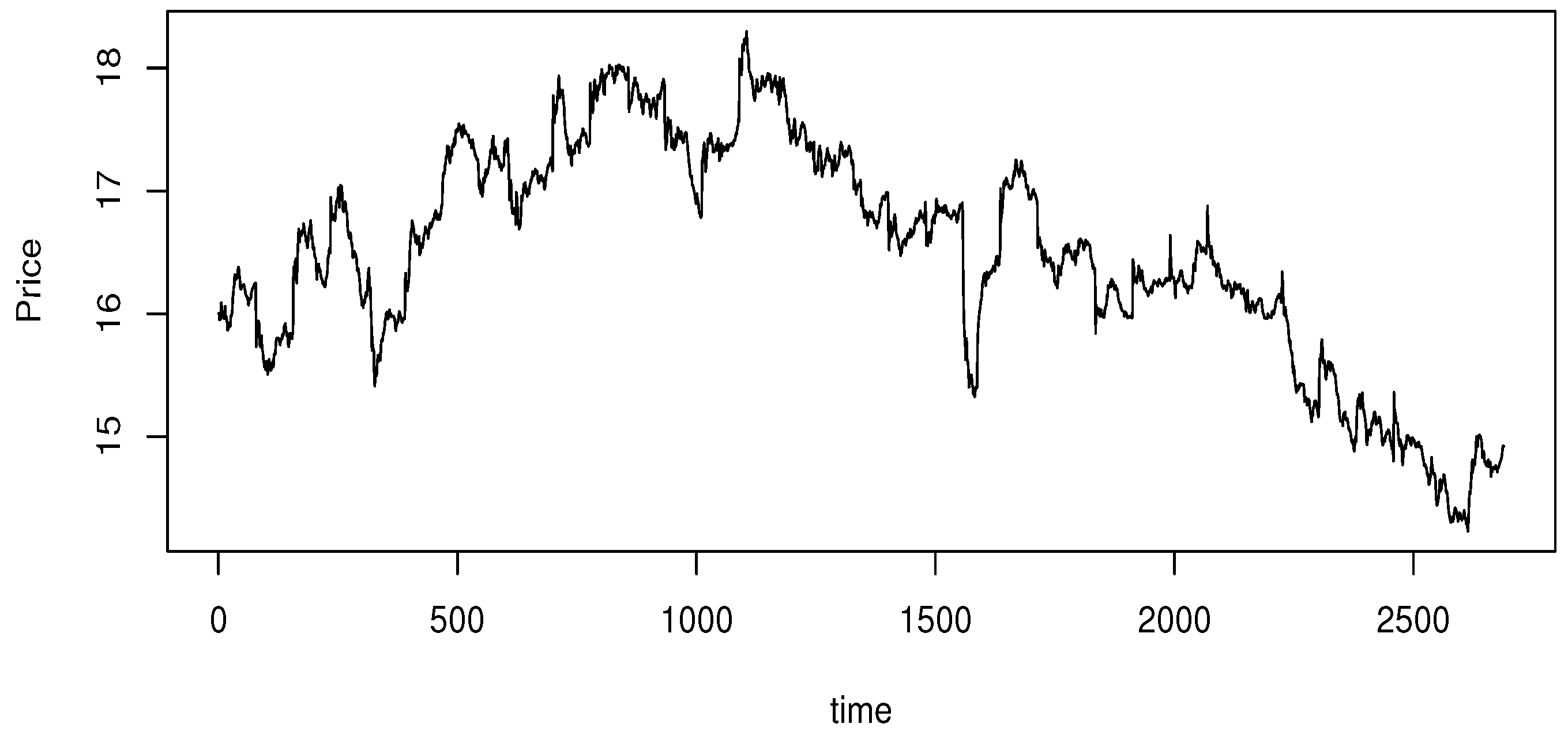
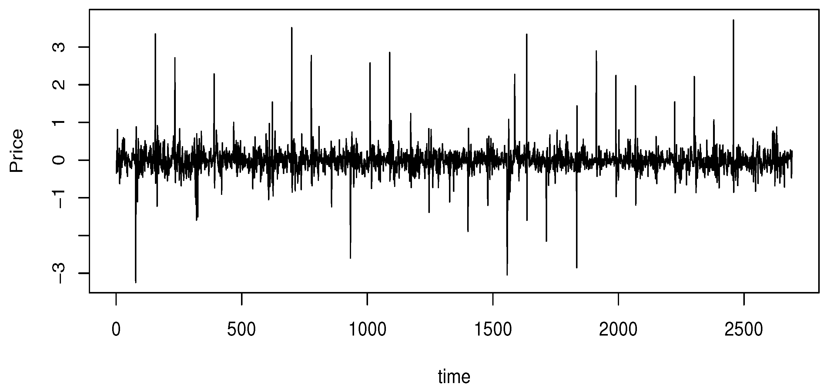
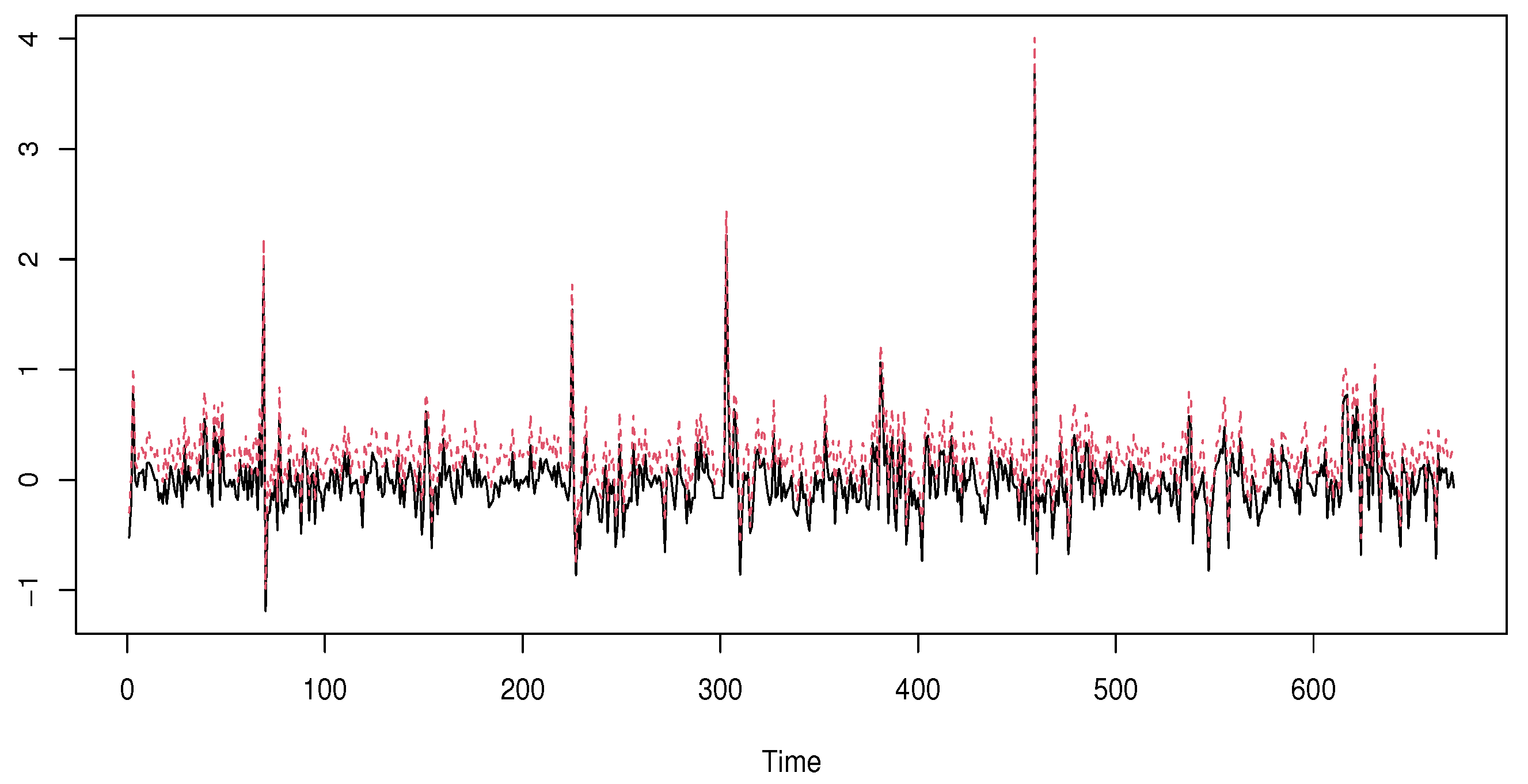
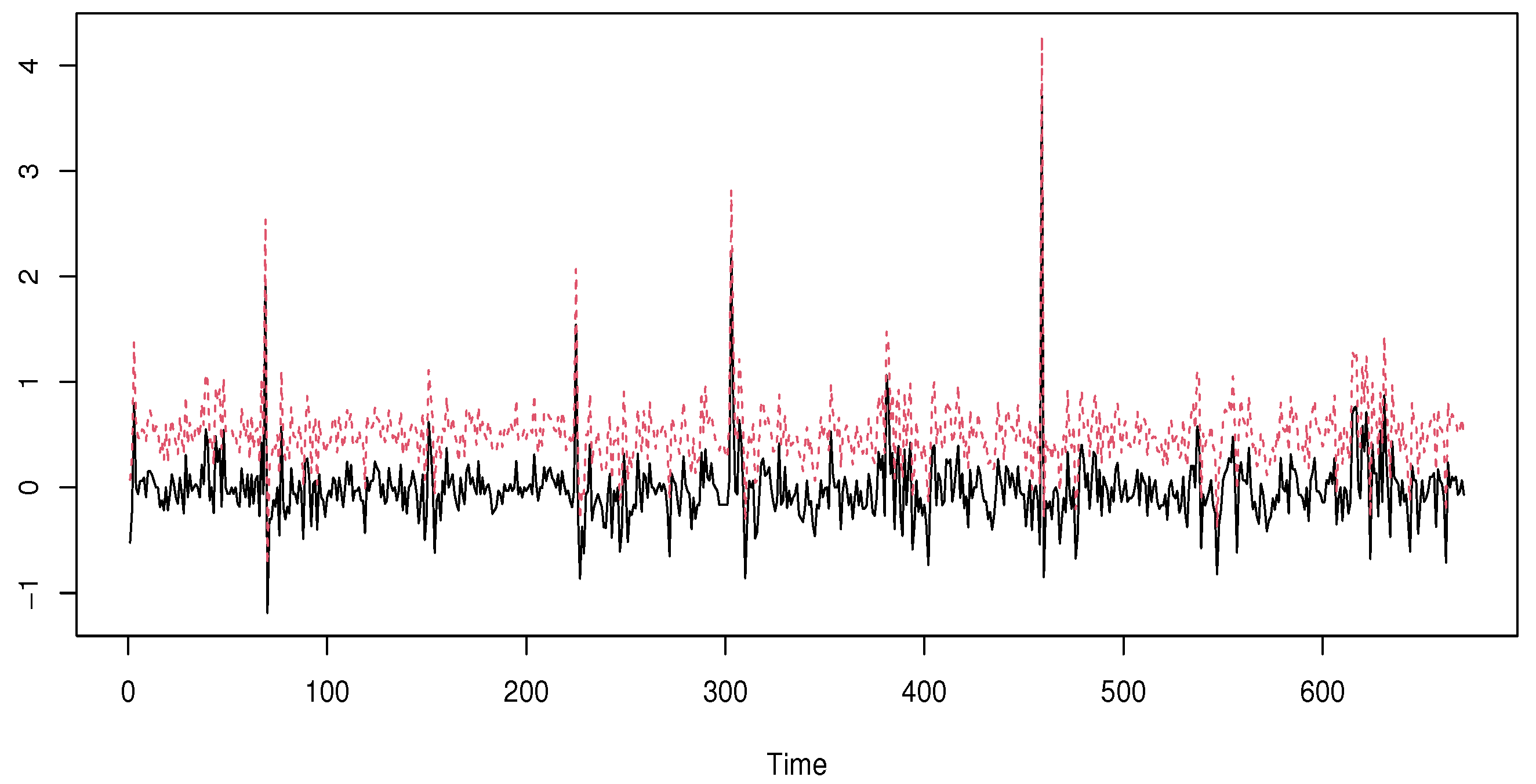
5.3. Real Data Application

This last paragraph is devoted to the applicability of our model to real data. More precisely, we examine the efficiency of the ES-expectile model over financial data associated with real-time stock prices of liberty energy company. This last is one of a major energy industry service provider across North America. Using these data, we compare our financial metric to its competitive ones. In this financial data analysis, we study the high price $P{\left(t\right)}_t$ of this company during October 2024, observed within a frame of five minutes. The parent data contains more than 2700 values. The process of $P{\left(t\right)}_t$ is displayed in Figure 2. It is available in https://stooq.com/db/l (accessed on 24 April 2024).

Figure 2. The high price $P\left(t\right)$.

To insure the stability, we proceeded with the difference algorithmic. We constructed the functional data from the process $R\left(t\right)=log\left(P\right(t+1)-log(P\left(t\right)\left)\right)$. The transformed data are given in Figure 3.

Figure 3. The process R(t).

We explore the functional path of the considered data by cutting the process $R\left(t\right)$ with pieces of 30 points. These pieces represent the functional regressors $A_i$. Furthermore, we use the same strategy as in the simulated data. Indeed, we choose $A_i$ as the curve of $R{\left(t\right)}_{t\in [s-30,s[}$ and $B_i=R\left(s\right)$. Now, to insure the independence structure of our work, we select distanced observations. Specifically, from 2790 observations, we choose 90 equidistant independent values from which we construct our learning sample ${(A_i,B_i)}_{i=1,\dots ,90}$. Thus, we compare the three estimators $\overline{CE{A}_p}$, $\widehat{CE{A}_p}$, and $\widetilde{CE{A}_p}$ using a real datum, ${(A_i,B_i)}_{i=1,\dots ,90}$. Such estimators are computed using the same algorithm of the simulated data. We use the same kernel and select the smoothing parameters k and h by the rule (6). We use the $L_2$ metric obtained by the PCA-metric. We refer to Ferraty and Vieu [31] for more details on the mathematical formulation of this metric. The comparison results are given in Figure 4, Figure 5 and Figure 6, where we plot the true values of 670 testing observations (black line) ${\left(B_i\right)}_{i=1,\dots ,670}$ versus the estimator $\widehat{CE{X}_p}\left(A_i\right)$ and $\widetilde{CE{A}_p}\left(A_i\right)$ (red line) for values of $p=0.1$.

Figure 4. kNN expectile expected shortfall.

Figure 5. kNN VaR expected shortfall.

Figure 6. Standard expectile expected shortfall.

Once again, the comparison confirms the superiority of the kNN ES-expectile regression over the standard ES-expectile and the kNN ES-quantile model. This superiority is confirmed by computing the Mse error (9) of the three models. We obtain, respectively, 0.0274 for the kNN ES-expectile, 0.108 for the standard ES-expectile 0.201, and for the kNN ES-quantile. For a deep examination of the behavior of the three estimators as financial risk models, we use the backtesting measure based on the cover test developed Bayer and Dimitriadis [32]. Specifically, we apply the version so-called one-side intercept expected shortfall regression backtest. This last is obtained using the routine code esr-backtest from the R-package esrback with $\alpha =0.05$. We compute the p-values of the 70 observations, randomly chosen, from the above 670 testing observations. The average of the obtained values confirms the first statement that is the kNN ES-expectile regression, which is more adequate than the standard ES-expectile and the kNN ES-quantile model. Specifically, the average of the p-values of the kNN ES-expectile is 0.035 against 0.067 for the standard ES-expectile, and for the 0.058 kNN ES- quantile.

6. Conclusions and Prospects

In the present work, we developed a free-parameter estimation of the ES-expectile-with-regression. We constructed an estimator using kNN smoothing. This study covers two principal aspects of the financial data analysis: In the theoretical part, we establish the almost complete convergence of the constructed estimator; moreover, to ensure the applicability of the constructed estimator, we also determine the convergence rate of the UCNN consistency. Of course, this theoretical analysis constitutes a good mathematical support for the use of the new developed risk-metric in practice. We point out that the obtained asymptotic results are established under standard conditions and with the precision of the convergence rate. In particular, all the assumed conditions are related to the functional structure of the regressors and the nonparametric path of the model. On the other hand, we observe that the applicability of the estimator is very easy and gives better results compared to the other financial risk metric. In addition, our contribution leaves many open questions. For instance, the first natural prospect is the treatment of the dependent case, which allows the control of the movement of the stock exchange in its natural path, that is, the functional time series case. The second future work is the establishment of the asymptotic distribution of our new estimator, which in both cases, are independent or dependent cases. Moreover, the third prospect concerns the determination of the single structure case. This last permit enables one to improve the convergence rate of the estimator. Furthermore, we can also treat the partial model case or the parametric case.

7. The Demonstration of the Intermediate Results

The proof of the intermediate results are regrouped in this Section.

Proof of Lemma 1. 

It suffices to apply Lemma 3 for $A_n^{-}\left(\zeta \right)={\varphi }^{-1}\left(\sqrt{\zeta }{\displaystyle \frac{k}{n}}\right)$, $A_n^{+}={\varphi }^{-1}\left({\displaystyle \frac{k}{\sqrt{\zeta }n}}\right)$ and $\mathfrak{L}(t,(z,{\mathfrak{Z}}_i))=\mathbf{F}\left[t^{-1}d(z,{\mathfrak{Z}}_i)\right]$ Since the choice of $A_n^{-}$, $A_n^{+}$ and $\mathfrak{L}$ are the same as in [27], Conditions (C1 and C2) are satisfied. So, all that remains is checking condition (C3). Indeed, by a simple decomposition, for $t\in \mathrm{I}\mathrm{R}$,

$$\widehat{CE}(t,s)-\widehat{CE}(t,s)={\displaystyle \frac{1}{{\widehat{CE}}_D\left(s\right)}}\left[\right({\widehat{CE}}_N(t,s)-\mathrm{I}\mathrm{E}\left[{\widehat{CE}}_N(t,s)\right])$$

$$-\left(\widehat{CE}(t,s))-\mathrm{I}\mathrm{E}\left[{\widehat{CE}}_N(t,s)\right]\right)]-{\displaystyle \frac{{\widehat{CE}}_N(t,s)}{{\widehat{CE}}_D\left(s\right)}}[{\widehat{CE}}_D\left(s\right)-\mathrm{I}\mathrm{E}\left[{\widehat{CE}}_D\left(s\right)\right]]$$

where

$${\widehat{CE}}_N(t,s)={\displaystyle \frac{1}{\mathrm{I}\mathrm{E}\left[\mathbf{F}\left[h^{-1}d(s,A_1)\right]\right]}}\sum _{i=1}^n\mathbf{F}\left[h^{-1}d(s,A_i)\right]B_i{\mathbb{1}}_{B_i>t}$$

$$\mathrm{and}{\widehat{CE}}_D\left(s\right)={\displaystyle \frac{1}{\mathrm{I}\mathrm{E}\left[\mathbf{F}\left[h^{-1}d(s,A_1)\right]\right]}}\sum _{i=1}^n\mathbf{F}\left[h^{-1}d(s,A_i)\right].$$

and $h=A_n^{-}$, or $a=A_n^{+}$ Therefore, (C3) is a consequence of

$${\widehat{CE}}_D\left(s\right)-\mathrm{I}\mathrm{E}\left[{\widehat{CE}}_D\left(s\right)\right]=O\left({\left({\displaystyle \frac{lnn}{n\varphi \left(h\right)}}\right)}^{1/2}\right)a.co.$$

$$\underset{t\in [{EXR}_p\left(s\right)-\delta ,{EXR}_p\left(s\right)+\delta ]}{sup}\left|{\widehat{CE}}_N(t,s)-\mathrm{I}\mathrm{E}\left[{\widehat{CE}}_N(t,s)\right]\right|=O\left({\left({\displaystyle \frac{lnn}{n\varphi \left(h\right)}}\right)}^{1/2}\right),a.co.$$

and

$$\underset{t\in [{EXR}_p\left(a\right)-\delta ,{EXR}_p\left(a\right)+\delta ]}{sup}\left|CE(t,s)-\mathrm{I}\mathrm{E}\left[{\widehat{CE}}_N(t,s)\right]\right|=O\left(h^b\right).$$

Because the proof of the three required results is based on similar analytical arguments in FDA, we only focus on the second results, namely,

$$\underset{t\in [{EXR}_p\left(a\right)-\delta ,{EXR}_p\left(a\right)+\delta ]}{sup}\left|{\widehat{CE}}_N(t,s)-\mathrm{I}\mathrm{E}\left[{\widehat{CE}}_N(t,s)\right]\right|=O\left({\left({\displaystyle \frac{lnn}{n\varphi \left(h\right)}}\right)}^{1/2}\right),a.co.$$

To do that, we write

$$[{EXR}_p\left(a\right)-\delta ,{EXR}_p\left(a\right)+\delta ]\subset \bigcup _{j=1}^{l_n}]B_j-d_n,y_j+d_n[$$

(10)

with ${\displaystyle d_n=O\left(\frac{1}{\sqrt{n}}\right)}$ and $l_n=O\left(\sqrt{n}\right)$. Since $\mathrm{I}\mathrm{E}\left[{\widehat{CE}}_N(·,s)\right]$ and ${\widehat{CE}}_N(·,s)$ are increasing functions. Thus, ∀$1\le j\le l_n$

$$\mathrm{I}\mathrm{E}{\widehat{CE}}_N(y_j-d_n,s)\le \underset{t\in ]y_j-d_n,y_j+d_n[}{sup}\mathrm{I}\mathrm{E}{\widehat{CE}}_N(t,s)\le \mathrm{I}\mathrm{E}{\widehat{CE}}_N(y_j+d_n,s)$$

$${\widehat{CE}}_N(t,s)(y_j-d_n,s)\le \underset{t\in ]y_j-d_n,y_j+d_n[}{sup}{\widehat{CE}}_N(t,s)\le {\widehat{CE}}_N(y_j+d_n,t).$$

(11)

Now, by (P2), we obtain

$$\underset{t\in [{EXR}_p\left(a\right)-\delta ,{EXR}_p\left(a\right)+\delta ]}{sup}\left|{\widehat{CE}}_N(t,s)-\mathrm{I}\mathrm{E}{\widehat{CE}}_N(t,s)\right|$$

$$\le \underset{1\le j\le l_n}{max}\underset{z\in \{y_j-d_n,y_j+d_n\}}{max}\left|{\widehat{CE}}_N(z,s)-\mathrm{I}\mathrm{E}{\widehat{CE}}_N(z,s)\right|+C{d}_n.$$

As

$$d_n=n^{-1/2}=o\left(\sqrt{{\displaystyle \frac{lnn}{n\varphi \left(h\right)}}}\right).$$

We treat

$$\underset{1\le j\le l_n}{max}\underset{z\in \{y_j-d_n,y_j+d_n\}}{max}\left|{\widehat{CE}}_N(z,s)-\mathrm{I}\mathrm{E}{\widehat{CE}}_N(z,s)\right|=O\left(\sqrt{{\displaystyle \frac{lnn}{n\varphi \left(h\right)}}}\right),a.co.$$

For this, we write for any $\eta >0$

$$\begin{array}{ccc}& & \mathrm{I}\mathrm{P}\left(\underset{1\le j\le l_n}{max}\underset{z\in \{y_j-d_n,y_j+d_n\}}{max}\left|{\widehat{CE}}_N(z,s)-\mathrm{I}\mathrm{E}{\widehat{CE}}_N(z,s)\right|>\eta \sqrt{{\displaystyle \frac{lnn}{n\varphi \left(h\right)}}}\right)\hfill \\ & & \le 2l_n\underset{1\le j\le l_n}{max}\underset{z\in \{y_j-d_n,y_j+d_n\}}{max}\mathrm{I}\mathrm{P}\left(\left|{\widehat{CE}}_N(z,s)-\mathrm{I}\mathrm{E}{\widehat{CE}}_N(z,s)\right|>\eta \sqrt{{\displaystyle \frac{lnn}{n\varphi \left(h\right)}}}\right).\hfill \end{array}$$

Now, we evaluate

$$\mathrm{I}\mathrm{P}\left(\left|{\widehat{CE}}_N(z,s)-\mathrm{I}\mathrm{E}{\widehat{CE}}_N(z,s)\right|>\eta \sqrt{{\displaystyle \frac{lnn}{n\varphi \left(h\right)}}}\right).$$

Indeed, let

$${\tilde{\mathbf{F}}}_i={\displaystyle \frac{1}{\mathrm{I}\mathrm{E}\left[\mathbf{F}\left[h^{-1}d(s,A_1)\right]\right]}}\left[\mathbf{F}\left[h^{-1}d(s,A_i)\right]B_{i}1{\mathrm{I}}_{\left\{B_i\le z\right\}}-\mathrm{I}\mathrm{E}\left[\mathbf{F}\left[h^{-1}d(s,A_i)\right]B_{i}1{\mathrm{I}}_{\left\{B_1\le z\right\}}\right]\right].$$

We write

$${\displaystyle \forall \epsilon >0,\mathrm{I}\mathrm{P}\left[|{\widehat{CE}}_N(z,s)-\mathrm{I}\mathrm{E}{\widehat{CE}}_N(z,s)|>\epsilon \right]=\mathrm{I}\mathrm{P}\left[\frac{1}{n}\left[\left|\sum _{i=1}^n{\tilde{\mathbf{F}}}_i\right|>\epsilon \right]\right]}$$

Since

$$\mathbb{E}|{\tilde{\mathbf{F}}}_i\left(a\right){|}^m=O\left({\left(\varphi \left(h\right)\right)}^{-m+1}\right).$$

(12)

we can apply the inequality of Bernstein with $a_n^2={\left(\varphi \left(h\right)\right)}^{-1},$ to obtain, for all $\tau >0$,

$$\begin{array}{ccc}\hfill \mathbb{P}\left(|{\widehat{CE}}_N(z,s)-\mathrm{I}\mathrm{E}{\widehat{CE}}_N(z,s)|>\tau \sqrt{{\displaystyle \frac{lnn}{n\varphi \left(h\right)}}}\right)& =& \mathbb{P}\left({\displaystyle \left|\sum _{i=1}^n{\tilde{\mathbf{F}}}_i\left(a\right)\right|>n\tau \sqrt{\frac{lnn}{n\varphi \left(h\right)}}}\right)\hfill \\ & \le & 2exp\left(-{\displaystyle \frac{1}{2}}{\displaystyle \frac{{\tau }^{2}lnn}{1+\tau \sqrt{\frac{lnn}{n\varphi \left(h\right)}}}}\right),\hfill \end{array}$$

Thus

$$\begin{array}{c}\hfill {\displaystyle \sum _{n\ge 1}\mathbb{P}\left(|{\widehat{CE}}_N(z,s)-\mathrm{I}\mathrm{E}{\widehat{CE}}_N(z,s)|>\tau \sqrt{\frac{lnn}{n\varphi \left(h\right)}}\right)\le 2\sum _{n\ge 1}exp\left(-C{\tau }^{2}lnn\right).}\end{array}$$

Thereby, for $\tau >{\displaystyle \frac{1}{\sqrt{C}}}$ gives

$$\left|{\widehat{CE}}_N(z,s)-\mathrm{I}\mathrm{E}{\widehat{CE}}_N(z,s)\right|=O_{a.co.}\left(\sqrt{{\displaystyle \frac{lnn}{n\varphi \left(h\right)}}}\right).$$

(13)

 □

Proof of Lemma 2. 

Let

$$z_n={\varphi }^{-1}{\left({\displaystyle \frac{k}{n}}\right)}^b+\sqrt{{\displaystyle \frac{lnn}{k}}}$$

Similarly to [19], we have

$$\begin{array}{c}{\displaystyle \sum _n\mathrm{I}\mathrm{P}\left(|{\widehat{EXR}}_p\left(a\right)-{EXR}_p\left(a\right)|>z_n\right)}\hfill \\ \le \sum _n\mathrm{I}\mathrm{P}\left(su{p}_{t\in [{EXR}_p\left(a\right)-\delta ,{EXR}_p\left(a\right)+\delta ]}|\tilde{G}(t,a)-G(t,a)|\ge C{z}_n\right)<\infty .\hfill \end{array}$$

where

$$G(t,a):={\displaystyle \frac{{\displaystyle G_1(t,a)}}{{\displaystyle G_2(t,a)}}},$$

with

$$\left\{\begin{array}{lll}{G}_1(t,a)& =& -\mathrm{I}\mathrm{E}\left[(B-t)1{\mathrm{I}}_{\left\{\right(B-t)\le 0\}}\mid A=a\right],\\ G_2(t,a)& =& \mathrm{I}\mathrm{E}\left[(b-t)1{\mathrm{I}}_{\left\{\right(B-t)>0\}}\mid A=a\right].\end{array}\right.$$

Therefore,

$$su{p}_{t\in [{EXR}_p\left(a\right)-\delta ,{EXR}_p\left(a\right)+\delta ]}\left|{\tilde{G}}_h(t,a)-G(t,a)\right|=O_{a.co.}\left(z_n\right).$$

(14)

Similarly to the previous lemma, we write

$$\begin{array}{ccc}\hfill {\tilde{G}}_h(t,a)-G(t,a)& =& {\displaystyle \frac{{\displaystyle {\tilde{G}}_1(t,a)}}{{\displaystyle {\tilde{G}}_2(t,a)}}}-{\displaystyle \frac{{\displaystyle G_1(t,a)}}{{\displaystyle G_2(t,a)}}}\hfill \\ \hfill & =& {\displaystyle \frac{{\displaystyle 1}}{{\displaystyle {\tilde{G}}_2(t,a)}}}\left[{\tilde{G}}_1(t,a)-G_1(t,a)\right]\hfill \\ & & +{\displaystyle \frac{{\displaystyle G(t,a)}}{{\displaystyle {\tilde{G}}_2(t,a)}}}\left[G_2(t,a)-{\tilde{G}}_2(t,a)\right],\hfill \end{array}$$

(15)

where

$${\tilde{G}}_1(t,a)=-{\displaystyle \frac{1}{n\mathrm{I}\mathrm{E}\left[{\mathbf{F}}_1\right]}}\sum _{i=1}^n{\mathbf{F}}_i(B_i-t)1{\mathrm{I}}_{\left\{\right(B_i-t)\le 0\}},$$

and

$${\tilde{G}}_2(t,a)=-{\displaystyle \frac{1}{n\mathrm{I}\mathrm{E}\left[{\mathbf{F}}_1\right]}}\sum _{i=1}^n{\mathbf{F}}_i(B_i-t)1{\mathrm{I}}_{\left\{\right(B_i-t)>0\}}.$$

We prove

$$su{p}_{t\in [{EXR}_p\left(a\right)-\delta ,{EXR}_p\left(a\right)+\delta ]}\left|{\widehat{G}}_1(t,a)-\mathrm{I}\mathrm{E}\left[{\widehat{G}}_1(t,a)\right]\right|=O_{a.co.}\left(z_n\right),$$

(16)

and

$$su{p}_{t\in [{EXR}_p\left(a\right)-\delta ,{EXR}_p\left(a\right)+\delta ]}\left|{\widehat{G}}_2(t,a)-\mathrm{I}\mathrm{E}\left[{\widehat{G}}_2(t,a)\right]\right|=O_{a.co.}\left(z_n\right).$$

(17)

The rest of the proof is based on the same arguments of Lemma 1 where $\widehat{CE}(t,a)$ is replaced by ${\widehat{G}}_1(t,a)$ or ${\widehat{G}}_2(t,a)$. □

Proof of Lemma 4. 

Let $\alpha \in ]0,1[$; thus, we write

$$\mathrm{I}\mathrm{P}\left\{{\displaystyle \underset{k_{1,n}\le k\le k_{2,n}}{sup}\underset{t\in [{EXR}_p\left(a\right)-\delta ,{EXR}_p\left(a\right)+\delta ]}{sup}\left|\widehat{CE}(t,a)-CE(t,a)\right|\ge z_n}\right\}$$

$$\le \mathrm{I}\mathrm{P}\left\{{\displaystyle \underset{k_{1,n}\le k\le k_{2,n}}{sup}\underset{t\in [{EXR}_p\left(a\right)-\delta ,{EXR}_p\left(a\right)+\delta ]}{sup}\left|\widehat{CE}(t,a)-CE(t,a)\right|\times 1{\mathrm{I}}_{\left\{{\varphi }^{-1}\left(\frac{\alpha k_{1,n}}{n}\right)\le h_k\le {\varphi }^{-1}\left(\frac{k_{2,n}}{n\alpha }\right)\right\}}\ge \frac{z_n}{2}}\right\}$$

$$+\mathrm{I}\mathrm{P}\left\{{\displaystyle h\notin \left({\varphi }^{-1}\left(\frac{\alpha k_{1,n}}{n}\right),{\varphi }^{-1}\left(\frac{k_{2,n}}{n\alpha }\right)\right)}\right\}.$$

It is shown, in [33], that

$${\displaystyle \sum _n\sum _{k=k_{1,n}}^{k_{2,n}}\mathrm{I}\mathrm{P}\left(h_k\le {\varphi }^{-1}\left(\frac{\alpha k_{1,n}}{n}\right)\right)<\infty \mathrm{and}\sum _n\sum _{k=k_{1,n}}^{k_{2,n}}\mathrm{I}\mathrm{P}\left(h_k\ge {\varphi }^{-1}\left(\frac{k_{2,n}}{n\alpha }\right)\right)<\infty .}$$

So, all that is left to be proven is

$$\begin{array}{c}\hfill {\displaystyle \underset{{\varphi }^{-1}\left(\frac{\alpha k_{1,n}}{n}\right)\le h\le {\varphi }^{-1}\left(\frac{k_{2,n}}{n\alpha }\right)}{sup}\underset{t\in [{EXR}_p\left(a\right)-\delta ,{EXR}_p\left(a\right)+\delta ]}{sup}\left|\widetilde{CE}(t,a)-CE(t,a)\right|=O_{a.co.}\left(z_n\right).}\end{array}$$

where $\widetilde{CE}(t,a)$ is obtained by replacing h by $A_{n,k}$ in $\widehat{CE}(t,a)$. For this aim, we use the following decomposition

$$\begin{array}{c}\hfill \widetilde{CE}(t,a)-CE(t,a)=\tilde{B}(t,a)+{\displaystyle \frac{\tilde{D}(t,a)}{{\widetilde{CE}}_D\left(a\right)}}+{\displaystyle \frac{\tilde{Q}(t,a)}{{\widetilde{CE}}_D\left(a\right)}},\end{array}$$

where

$$\begin{array}{ccc}\hfill \tilde{Q}(t,a)& =& {\displaystyle ({\widetilde{CE}}_N(t,a)-\mathrm{I}\mathrm{E}[{\widetilde{CE}}_N(t,a)])-CE(t,a)({\widetilde{CE}}_D(a)-\mathrm{I}\mathrm{E}[{\widetilde{CE}}_D(a)]),}\hfill \\ \hfill \tilde{B}(t,a)& =& {\displaystyle \frac{\mathrm{I}\mathrm{E}[{\widetilde{CE}}_N(t,a)]}{\mathrm{I}\mathrm{E}[{\widetilde{CE}}_D(a)]}-CE(t,a)\mathrm{and}\tilde{D}(t,a)=-\tilde{B}(t,a)({\widetilde{CE}}_D(a)-\mathrm{I}\mathrm{E}[{\widetilde{CE}}_D(a)]),}\hfill \end{array}$$

with

$${\widetilde{CE}}_N(t,a)={\displaystyle \frac{1}{n\varphi \left(h\right)}}\sum _{i=1}^n\mathbf{F}\left[h^{-1}d(a,A_i)\right]B_i{\mathbb{1}}_{B_i>t}$$

and

$${\widetilde{CE}}_D\left(a\right)={\displaystyle \frac{1}{n\varphi \left(h\right)}}\sum _{i=1}^n\mathbf{F}\left[h^{-1}d(a,A_i)\right].$$

Thus, we split the proof of Lemma 4 into

$$\underset{a_n\le h\le b_n}{sup}\left|{\widetilde{CE}}_D\left(a\right)-\mathrm{I}\mathrm{E}\left[{\widetilde{CE}}_D\left(a\right)\right]\right|=O_{a.co.}\left(\sqrt{{\displaystyle \frac{lnn}{n\varphi \left(a_n\right)}}}\right).$$

$$\underset{a_n\le h\le b_n}{sup}\underset{t\in [{EXR}_p\left(a\right)-\delta ,{EXR}_p\left(a\right)+\delta ]}{sup}\left|{\widetilde{CE}}_N(t,a)-\mathrm{I}\mathrm{E}\left[{\widetilde{CE}}_N(t,a)\right]\right|=O_{a.co.}\left(\sqrt{{\displaystyle \frac{lnn}{n\varphi \left(a_n\right)}}}\right),$$

where ${\displaystyle a_n={\varphi }^{-1}\left(\frac{\alpha k_{1,n}}{n}\right)}$ and $b_n={\varphi }^{-1}\left({\displaystyle \frac{k_{2,n}}{n\alpha }}\right)$.

We concentrate on the second convergence. The first one can be deduced by the same tools. Indeed, we write that

$$\begin{array}{c}\hfill [{EXR}_p\left(a\right)-\delta ,{EXR}_p\left(a\right)+\delta ]\subset \bigcup _{j=1}^{d_n}\left(t_j-l_n,t_j+l_n\right),\end{array}$$

with ${\displaystyle l_n=n^{-1/2}}$ and $d_n=O\left(n^{1/2}\right)$.

Next, since the functions $\mathrm{I}\mathrm{E}\left[{\widetilde{CE}}_N(x,·)\right]$ and ${\widetilde{CE}}_N(x,·)$ are monotone, which implies that, for $1\le j\le d_n$,

$$\begin{array}{ccc}\hfill \mathrm{I}\mathrm{E}\left[{\widetilde{CE}}_N(x,t_j-l_n)\right]& \le & \underset{t\in (t_j-l_n,t_j+l_n)}{sup}\mathrm{I}\mathrm{E}\left[{\widetilde{CE}}_N(t,a)\right]\le \mathrm{I}\mathrm{E}\left[{\widetilde{CE}}_N(x,t_j+l_n)\right],\hfill \\ \hfill {\widetilde{CE}}_N(x,t_j-l_n)& \le & \underset{t\in (t_j-l_n,t_j+l_n)}{sup}{\widetilde{CE}}_N(t,a)\le {\widetilde{CE}}_N(x,t_j+l_n).\hfill \end{array}$$

Thus

$$\begin{array}{c}{\displaystyle \underset{t\in [{EXR}_p\left(a\right)-\delta ,{EXR}_p\left(a\right)+\delta ]}{sup}\left|{\widetilde{CE}}_N(t,a)-\mathrm{I}\mathrm{E}\left[{\widetilde{CE}}_N(t,a)\right]\right|}\\ \le \underset{1\le j\le d_n}{max}\underset{z\in \{t_j-l_n,t_j+l_n\}}{max}\left|{\widetilde{CE}}_N(z,a)-\mathrm{I}\mathrm{E}\left[{\widetilde{CE}}_N(z,a)\right]\right|+2C{l}_n.\hfill \end{array}$$

Observe that ${\displaystyle l_n=o{\left(\frac{lnn}{n\varphi \left(a_n\right)}\right)}^{1/2}.}$ Now, it suffices to

$$\underset{a_n\le h\le b_n}{sup}\underset{1\le j\le d_n}{max}\underset{z\in \{t_j-l_n,t_j+l_n\}}{max}\left|{\widetilde{CE}}_N(x,z)-\mathrm{I}\mathrm{E}\left[{\widetilde{CE}}_N(x,z)\right]\right|=O{\left({\displaystyle \frac{lnn}{n\varphi \left(a_n\right)}}\right)}^{1/2},a.co.$$

(18)

For this, we write that

$$\begin{array}{c}{\displaystyle \mathrm{I}\mathrm{P}\left(\underset{a_n\le h\le b_n}{sup}\underset{1\le j\le d_n}{max}\underset{z\in \{t_j-l_n,t_j+l_n\}}{max}\left|{\widetilde{CE}}_N(x,z)-\mathrm{I}\mathrm{E}\left[{\widetilde{CE}}_N(x,z)\right]\right|>\eta \sqrt{\frac{lnn}{n\varphi \left(a_n\right)}}\right)}\\ \le 2d_n\underset{1\le j\le d_n}{max}\underset{z\in \{t_j-l_n,t_j+l_n\}}{max}\mathrm{I}\mathrm{P}\left(\underset{a_n\le h\le b_n}{sup}\left|{\widetilde{CE}}_N(x,z)-\mathrm{I}\mathrm{E}\left[{\widetilde{CE}}_N(x,z)\right]\right|>\eta \sqrt{{\displaystyle \frac{lnn}{n\varphi \left(a_n\right)}}}\right).\end{array}$$

We evaluate the following quantity

$$\mathrm{I}\mathrm{P}\left(\underset{a_n\le h\le b_n}{sup}\left|{\widetilde{CE}}_N(x,z)-\mathrm{I}\mathrm{E}\left[{\widetilde{CE}}_N(x,z)\right]\right|>\eta \sqrt{{\displaystyle \frac{lnn}{n\varphi \left(a_n\right)}}}\right), \mathrm{for} \mathrm{all} z=t_j\mp l_n,1\le j\le d_n.$$

The proof of the latter is based on Bernstein’s inequality for empirical processes as in [33]. The empirical processes are

$${\alpha }_n\left(\mathcal{K}\right)={\displaystyle \frac{1}{\sqrt{n}}}\sum _{i=1}^n\left({\mathcal{F}}_{i}1{\mathrm{I}}_{\left\{B_i\ge t\right\}}-\mathrm{I}\mathrm{E}\left[{\mathcal{F}}_{i}1{\mathrm{I}}_{\left\{B_i\ge t\right\}}\right]\right).$$

where ${\mathcal{F}}_i=\mathbf{F}\left[h^{-1}d(a,A_i)\right]$. Thereafter, we obtain

$$\mathrm{I}\mathrm{P}\left(\underset{a_n\le h\le b_0}{sup}\sqrt{{\displaystyle \frac{n\varphi \left(h\right)}{lnn}}}\left|{\widetilde{CE}}_N(z,a)-\mathrm{I}\mathrm{E}\left[{\widetilde{CE}}_N(z,a)\right]\right|\ge {\eta }_0^{\prime }\right)\le ln\left(n\right)n^{-C^{\prime }{\eta }_0^2}.$$

Consequently, an adequate choice of ${\eta }_0$ enables us to deduce (18). □

References

- Artzner, P.; Delbaen, F.; Eber, J.M.; Heath, D. Coherent measures of risk. Math. Financ. 1999, 9, 203–228. [Google Scholar] [CrossRef]
- Righi, M.B.; Ceretta, P.S. A comparison of expected shortfall estimation models. J. Econ. Bus. 2015, 78, 14–47. [Google Scholar] [CrossRef]
- Moutanabbir, K.; Bouaddi, M. A new non-parametric estimation of the expected shortfall for dependent financial losses. J. Stat. Plan. Inference 2024, 232, 106151. [Google Scholar] [CrossRef]
- Lazar, E.; Pan, J.; Wang, S. On the estimation of Value-at-Risk and Expected Shortfall at extreme levels. J. Commod. Mark. 2024, 3, 100391. [Google Scholar] [CrossRef]
- Scaillet, O. Nonparametric estimation and sensitivity analysis of expected shortfall. Math. Financ. Int. J. Math. Stat. Financ. Econ. 2004, 14, 115–129. [Google Scholar] [CrossRef]
- Cai, Z.; Wang, X. Nonparametric estimation of conditional VaR and expected shortfall. J. Econom. 2008, 147, 120–130. [Google Scholar] [CrossRef]
- Wu, Y.; Yu, W.; Balakrishnan, N.; Wang, X. Nonparametric estimation of expected shortfall via Bahadur-type representation and Berry–Esséen bounds. J. Stat. Comput. Simul. 2022, 92, 544–566. [Google Scholar] [CrossRef]
- Ferraty, F.; Quintela-Del-Río, A. Conditional VAR and expected shortfall: A new functional approach. Econom. Rev. 2016, 35, 263–292. [Google Scholar] [CrossRef]
- Ait-Hennani, L.; Kaid, Z.; Laksaci, A.; Rachdi, M. Nonparametric estimation of the expected shortfall regression for quasi-associated functional data. Mathematics 2022, 10, 4508. [Google Scholar] [CrossRef]
- Newey, W.K.; Powell, J.L. Asymmetric least squares estimation and testing. Econom. J. Econom. Soc. 1987, 55, 819–847. [Google Scholar] [CrossRef]
- Waltrup, L.S.; Sobotka, F.; Kneib, T.; Kauermann, G. Expectile and quantile regression—David and Goliath? Stat. Model. 2015, 15, 433–456. [Google Scholar] [CrossRef]
- Bellini, F.; Di Bernardino, E. Risk management with expectiles. Eur. J. Financ. 2017, 23, 487–506. [Google Scholar] [CrossRef]
- Farooq, M.; Steinwart, I. Learning rates for kernel-based expectile regression. Mach. Learn. 2019, 108, 203–227. [Google Scholar] [CrossRef]
- Bellini, F.; Negri, I.; Pyatkova, M. Backtesting VaR and expectiles with realized scores. Stat. Methods Appl. 2019, 28, 119–142. [Google Scholar] [CrossRef]
- Chakroborty, S.; Iyer, R.; Trindade, A.A. On the use of the M-quantiles for outlier detection in multivariate data. arXiv 2024, arXiv:2401.01628. [Google Scholar]
- Gu, Y.; Zou, H. High-dimensional generalizations of asymmetric least squares regression and their applications. Ann. Stat. 2016, 44, 2661–2694. [Google Scholar] [CrossRef]
- Zhao, J.; Chen, Y.; Zhang, Y. Expectile regression for analyzing heteroscedasticity in high dimension. Stat. Probab. Lett. 2018, 137, 304–311. [Google Scholar] [CrossRef]
- Kneib, T. Beyond mean regression. Stat. Model. 2013, 13, 275–303. [Google Scholar] [CrossRef]
- Mohammedi, M.; Bouzebda, S.; Laksaci, A. The consistency and asymptotic normality of the kernel type expectile regression estimator for functional data. J. Multivar. Anal. 2021, 181, 104673. [Google Scholar] [CrossRef]
- Girard, S.; Stupfler, G.; Usseglio-Carleve, A. Functional estimation of extreme conditional expectiles. Econom. Stat. 2022, 21, 131–158. [Google Scholar] [CrossRef]
- Almanjahie, I.M.; Bouzebda, S.; Kaid, Z.; Laksaci, A. The local linear functional kNN estimator of the conditional expectile: Uniform consistency in number of neighbors. Metrika 2024, 1–29. [Google Scholar] [CrossRef]
- Aneiros, G.; Cao, R.; Fraiman, R.; Genest, C.; Vieu, P. Recent advances in functional data analysis and high-dimensional statistics. H. Multivar. Anal. 2019, 170, 3–9. [Google Scholar] [CrossRef]
- Goia, A.; Vieu, P. An introduction to recent advances in high/infinite dimensional statistics. J. Multivar. Anal. 2016, 170, 1–6. [Google Scholar] [CrossRef]
- Yu, D.; Pietrosanu, M.; Mizera, I.; Jiang, B.; Kong, L.; Tu, W. Functional Linear Partial Quantile Regression with Guaranteed Convergence for Neuroimaging Data Analysis. Stat. Biosci. 2024, 1–17. [Google Scholar] [CrossRef]
- Di Bernardino, E.; Laloe, T.; Pakzad, C. Estimation of extreme multivariate expectiles with functional covariates. J. Multivar. Anal. 2024, 202, 105292. [Google Scholar] [CrossRef]
- Collomb, G.; Härdle, W.; Hassani, S. A note on prediction via conditional mode estimation. J. Statist. Plann. Inference 1987, 15, 227–236. [Google Scholar] [CrossRef]
- Burba, F.; Ferraty, F.; Vieu, P. k-nearest neighbor method in functional nonparametric regression. J. Nonparametr. Statist. 2009, 21, 453–469. [Google Scholar] [CrossRef]
- Kudraszow, N.; Vieu, P. Uniform consistency of kNN regressors for functional variables. Statist. Probab. Lett. 2013, 83, 1863–1870. [Google Scholar] [CrossRef]
- Bouzebda, S.; Nezzal, A. Uniform consistency and uniform in number of neighbors consistency for nonparametric regression estimates and conditional U-statistics involving functional data. Jpn. J. Stat. Data Sci. 2022, 5, 431–533. [Google Scholar] [CrossRef]
- Bouzebda, S.; Mohammedi, M.; Laksaci, A. The k-nearest neighbors method in single index regression model for functional quasi-associated time series data. Rev. Mat. Complut. 2022, 36, 361–391. [Google Scholar] [CrossRef]
- Ferraty, F.; Vieu, P. Nonparametric Functional Data Analysis; Springer Series in Statistics; Springer: New York, NY, USA, 2006. [Google Scholar]
- Bayer, S.; Dimitriadis, T. Regression-Based Expected Shortfall Backtesting. J. Financ. Econom. 2022, 20, 437–471. [Google Scholar] [CrossRef]
- Kara-Zaïtri, L.; Laksaci, A.; Rachdi, M.; Vieu, P. Data-driven kNN estimation for various problems involving functional data. J. Multivariate Anal. 2017, 153, 176–188. [Google Scholar] [CrossRef]
Disclaimer/Publisher’s Note: The statements, opinions and data contained in all publications are solely those of the individual author(s) and contributor(s) and not of MDPI and/or the editor(s). MDPI and/or the editor(s) disclaim responsibility for any injury to people or property resulting from any ideas, methods, instructions or products referred to in the content. |
© 2024 by the authors. Licensee MDPI, Basel, Switzerland. This article is an open access article distributed under the terms and conditions of the Creative Commons Attribution (CC BY) license (https://creativecommons.org/licenses/by/4.0/).