Closed-Form Solutions for Kermack–McKendrick Dynamical System

Abstract

This work offers a (semi-analytical) solution for a second-order nonlinear differential equation associated to the dynamical Kermack–McKendrick system. The approximate closed-form solutions are obtained by means of the Optimal Homotopy Asymptotic Method (OHAM) using only one iteration. These solutions represent the $\epsilon$-approximate OHAM solutions. The advantages of this analytical procedure are reflected by comparison between the analytical solutions, numerical results, and corresponding iterative solutions (via a known iterative method). The obtained results are in a good agreement with the exact parametric solutions and corresponding numerical results, and they highlight that our procedure is effective, accurate, and useful for implementation in applications.

1. Introduction

In order to understand the threshold between the disappearance of disease and epidemic outbreak, mathematical models and numerical simulations are a necessity [1]. A basic model is given by the Kermack–McKendrick system, which describes the spread of infection within a population in a function of time. The total population is constant, and it is divided into three distinct groups: first, the exposed individuals (susceptible); second, the infected population who can further transmit the disease; and last, the individuals who already had the disease and cannot be infected or infect the others. The Susceptible–Infected–Recovered (SIR) epidemic model was analytically approached by Harko et al. [2] using the Laplace–Adomian decomposition method, resulting in establishing the exact analytical solution of SIR in a parametric form [3].

Semendyaeva et al. [4] evaluated analytically and numerically the SIR model regarding the COVID-19 propagation dynamic. Prodanov [5] highlighted some computational aspects of the SIR model used for the COVID-19 outbreaks. Furthermore, Pakes [6] extended the deterministic SIR model, resulting in the possibility of infected individuals becoming susceptible once again.

MacFarlane [7] developed a dynamic structure theory based on the relationships between the structure of ecosystems, social systems, or physiological functions characterized by several parameters. Motee et al. [8] investigated the asymptotic stability properties of a class of quasi-polynomial dynamical systems with applications in various biochemical and biological systems. Toledo–Hernandez et al. [9,10] studied the behavior of fermentation and thermal hydrolysis reactive systems. Figueiredo et al. [11] discussed simple examples of biological regulatory networks using a well-developed computational tool, differential dynamic logic $\left(d\mathcal{L}\right)$. Liu et al. [12] designed a new conservative hyperchaotic system and dynamic biogenetic gene algorithms, proposing a novel image encryption algorithm. Cheung et al. [13] developed an optimization algorithm, a human readable fuzzy rule-based model, for two dynamic biological networks. Daun et al. [14] reviewed differential equations as a simulation tool in the biological and clinical sciences, including their assumptions, strengths, and weaknesses, based on inference and empirical data analysis. Malchow [15] approached analytical and numerical investigations of well-known models from population dynamics and chemical physics. Liu et al. [16] proposed a computationally effective fractional Predictor–Corrector method for a dynamical model of competence induction in a cell with measurement error and noisy data. Gulati et al. [17] discussed the optimization of the biological control strategies to study global stability analysis using a Lyapunov function. Al-Nassir [18] examined the dynamic behavior of the fractional-order prey–predator system and its discretization with harvesting on prey species, using the discrete version of the Pontryagin maximum principle. Lampartova et al. [19] designed a classification of trajectories of explored systems, reflecting persistence, regularity, chaos, intermittency, and transiency. They investigated dynamical properties such as stability, dissipativity, and the stability of feedback interconnections using linear Lyapunov functions. Francis et al. [20] used the Routh–Hurwitz (RH) criterion and the eigenvalue technique to study the local stabilities of multi-species ecological systems.

The paper is organized in six sections: following the Introduction, Section 2 presents the Kermack–McKendrick system. Section 3 is dedicated to the Optimal Homotopy Asymptotic Method. Section 4 develops semi-analytical solutions via the OHAM technique, while Section 5 contains the numerical results and validation through comparison with iterative solutions and corresponding exact parametric solutions. The final Section 6 summarizes the concluding remarks.

2. The Dynamical Kermack–McKendrick System

The epidemic model was first introduced by Kermack et al. [21], wherein it is considered that the total population is constant (the Hamiltonian of the system), and it is divided into three distinct groups represented by x, y, and z. The dynamical Kermack–McKendrick system is written as [22]:

$$\left\{\begin{array}{c}\dot{x}=-axy\hfill \\ \dot{y}=axy-by\hfill \\ \dot{z}=by\hfill \end{array}\right.,a,b>0,$$

(1)

where a is the infection rate, b is the removal rate of the infected subjects, $x=x\left(t\right)$ denotes the number of individuals who can catch the disease, named the susceptible, $y=y\left(t\right)$ denotes the number of individuals who have the disease and can transmit it, and $z=z\left(t\right)$ denotes the number of individuals who had the disease, cannot be reinfected, and cannot infect other individuals.

The system (1) is a Hamiltonian mechanical system, having a Hamiltonian–Poisson structure characterized by the constants of motion given by:

$$\begin{array}{c}H(x,y,z)=x+y+z\mathrm{the}\mathrm{Hamiltonian},\hfill \\ C(x,y,z)=ln\left|x\right|+\frac{a}{b}z\mathrm{the}\mathrm{Casimir},\hfill \end{array}$$

(2)

with $x\ne 0$.

Considering the initial conditions

$$x\left(0\right)=x_0,y\left(0\right)=y_0,z\left(0\right)=z_0,$$

(3)

the exact solution of Equations (1) and (3) is written as the intersection of the surfaces:

$$\left\{\begin{array}{c}x+y+z=x_0+y_0+z_0\hfill \\ ln\left|x\right|+\frac{a}{b}z=ln\left|x_0\right|+\frac{a}{b}{z}_0\hfill \end{array}\right.,$$

(4)

for $x_0\ne 0$.

The trivial case $x_0=0$ is neglected.

Taking into account Equation (2), it is more convenient to consider the transformation

$$\left\{\begin{array}{c}x=x_0{e}^{-\frac{a}{b}u}\hfill \\ y=\frac{1}{b}\dot{u}\hfill \\ z-z_0=u\hfill \end{array}\right.,$$

(5)

which describes the closed-form solutions of Equations (1) and (3). The unknown smooth function u from Equation (5) is a solution of the nonlinear initial value problem:

$$\left\{\begin{array}{c}\ddot{u}+b\dot{u}-a{x}_0{e}^{-\frac{a}{b}u}\dot{u}=0\hfill \\ u\left(0\right)=0,\dot{u}\left(0\right)=b{y}_0,\hfill \end{array}\right.$$

(6)

obtained from the second Equation (1).

In Section 4 are presented some semi-analytical solutions of Equation (6) using the OHAM procedure, denoted by $\overline{u}$ or ${\overline{u}}_{OHAM}$.

Taking into consideration Equation (5), the semi-analytical closed-form solutions of the Equations (1) and (3) are

$$\left\{\begin{array}{c}\overline{x}=x_0{e}^{-\frac{a}{b}\overline{u}}\hfill \\ \overline{y}=\frac{1}{b}\dot{\overline{u}}\hfill \\ \overline{z}=z_0+\overline{u}\hfill \end{array}\right.,$$

(7)

where $\overline{u}$ is a semi-analytical solution of Equation (6).

3. The Idea of Optimal Homotopy Asymptotic Method

The OHAM technique is an analytical method to build approximate solutions. The dynamic system is reduced to a second-order nonlinear ordinary differential equation which is solved analytically with the OHAM method.

The nonlinear differential equation is assumed as [23]:

$$\mathcal{L}\left(F\left(t\right)\right)+\mathcal{N}\left(F\left(t\right)\right)=0,$$

(8)

with the initial condition (for $t=0$)

$$\mathcal{B}\left(F\left(0\right),\frac{dF\left(0\right)}{dt}\right)=0,$$

(9)

where $\mathcal{L}$ is an arbitrary linear operator, $\mathcal{N}$ is the corresponding nonlinear operator, $F\left(t\right)$ is the unknown smooth function, and $\mathcal{B}$ is an operator characterizing the boundary conditions.

The residual function depending on the approximate solution $\tilde{F}\left(t\right)$ of Equation (8) is given by:

$$\mathcal{R}(t,\tilde{F})=\mathcal{L}\left(\tilde{F}\left(t\right)\right)+\mathcal{N}\left(\tilde{F}\left(t\right)\right),t>0.$$

(10)

For $p\in [0,1]$, an embedding parameter, and $\mathrm{\Phi }(t,p)$, an unknown function, the homotopic relation has the form:

$$\begin{array}{c}\mathcal{H}\left[\mathcal{L}\left(\mathrm{\Phi }(t,p)\right),H(t,C_i),\mathcal{N}\left(\mathrm{\Phi }(t,p)\right)\right]=\hfill \\ \\ =\mathcal{L}\left(F_0\left(t\right)\right)+p\left[\mathcal{L}\left(F_1(t,C_i)\right)-H(t,C_i)\mathcal{N}\left(F_0\left(t\right)\right)\right]=0,\hfill \end{array}$$

(11)

where $H(t,C_i)\ne 0$ is an auxiliary convergence control function depending on the variable t and the unknown parameters $C_1$, $C_2$, …, $C_s$; and $F_0\left(t\right)$ denotes the initial approximation function and $F_1(t,C_i)$ denotes the first approximation function, respectively, of the exact solution $F\left(t\right)$.

If p increases from 0 to 1, then the solution $\mathrm{\Phi }(t,p)$ of Equation (8) varies from $\mathrm{\Phi }(t,0)=F_0\left(t\right)$ to the solution $\mathrm{\Phi }(t,1)=F\left(t\right)$ of Equation (8).

Considering the unknown function $\mathrm{\Phi }(t,p)$ in the form:

$$\mathrm{\Phi }(t,p)=F_0\left(t\right)+p{F}_1(t,C_i),$$

(12)

and equating the coefficients of $p^0$ and $p^1$, respectively, the following deformation problems are obtained:

-

The zeroth-order deformation problem

$$\mathcal{L}\left(F_0\left(t\right)\right)=0,\mathcal{B}\left(F_0\left(0\right),\frac{d{F}_0\left(0\right)}{dt}\right)=0,$$

(13)

whose solution is the initial approximation function $F_0\left(t\right)$.

-

The first-order deformation problem

$$\begin{array}{c}\mathcal{L}\left(F_1(t,C_i)\right)=H(t,C_i)\mathcal{N}\left(F_0\left(t\right)\right),\hfill \\ \\ \mathcal{B}\left(F_1(0,C_i),\frac{d{F}_1(0,C_i)}{dt}\right)=0,i=1,2,\cdots ,s,\hfill \end{array}$$

(14)

with solution the first approximation function $F_1(t,C_i)$.

On the other hand, to obtain $F_1(t,C_i)$ from Equation (14), the nonlinear operator $\mathcal{N}$ is assumed to have the general form:

$$\begin{array}{c}{\displaystyle \mathcal{N}\left(F_0\left(t\right)\right)=\sum _{i=1}^n{h}_i\left(t\right)g_i\left(t\right),}\hfill \end{array}$$

(15)

where n is a positive integer, and $h_i\left(t\right)$ and $g_i\left(t\right)$ are known elementary functions that depend on $F_0\left(t\right)$ and $\mathcal{N}$.

To compute the function $F_1(t,C_i)$, we consider the method presented in [23], and the following form is obtained:

$$\begin{array}{c}{F}_1(t,C_i)={\sum }_{i=1}^m{H}_i(t,h_j\left(t\right),C_j)g_i\left(t\right),j=1,\cdots ,s,\hfill \end{array}$$

(16)

or

$$\begin{array}{c}{F}_1(t,C_i)={\sum }_{i=1}^m{H}_i(t,g_j\left(t\right),C_j)h_i\left(t\right),j=1,\cdots ,s,\hfill \\ \\ \mathcal{B}\left(F_1(t,C_i),\frac{d{F}_1(t,C_i)}{dt}\right)=0,\hfill \end{array}$$

(17)

with $H_i(t,h_j\left(t\right),C_j)$—linear combination of the functions $h_j$, $j=1,\dots ,s$ and the parameters $C_j$, $j=1,\dots ,s$. The summation limit m is an arbitrary positive integer number.

For $p=1$, the first-order analytical approximate solution of Equations (8) and (9), taking into account Equation (12), has the form:

$$\tilde{F}(t,C_i)=\mathrm{\Phi }(t,1)=F_0\left(t\right)+F_1(t,C_i),$$

(18)

where $\tilde{F}(t,C_i)$ is a real linear combination of these functions $h_j$.

The unknown parameters $C_1$, $C_2$, …, $C_s$ can be optimally computed by means of various methods, such as the weighted residual method, the Kantorowich method, the least square method, the Galerkin method, and the collocation method.

The first-order approximate solution (18) is well-determined if the convergence control parameters $C_1$, $C_2$, …, $C_s$ are known.

Some mathematical notions, such as OHAM sequence, OHAM functions, $\epsilon$-approximate OHAM solutions, and weak $\epsilon$-approximate OHAM solutions, are defined in [24]. Theorem 1, introduced after these definitions, emphasizes the existence of weak $\epsilon$-approximate OHAM solutions.

4. Semi-Analytical Solutions via OHAM Technique

The applicability of the OHAM method for the nonlinear differential problems given by Equation (6) is pointed out in this section. This problem has the form of Equation (8), using the following operators:

$$\begin{array}{c}{\displaystyle \mathcal{L}\left[u\left(t\right)\right]=\ddot{u}\left(t\right)+K\dot{u}\left(t\right)}\hfill \\ {\displaystyle \mathcal{N}[t,u\left(t\right),\dot{u}\left(t\right),\ddot{u}\left(t\right)]=(b-K)\dot{u}\left(t\right)-a{x}_0{e}^{-\frac{a}{b}u\left(t\right)}\dot{u}\left(t\right),t>0,}\hfill \end{array}$$

(19)

where $K>0$ is unknown parameter at this moment.

The semi-analytical solution of Equation (6) is constructed using the follow expand series:

$${\displaystyle e^{u\left(t\right)}=\sum _{n=0}^{\infty }\frac{1}{n!}{u}^n\left(t\right)=1+\frac{1}{1!}u\left(t\right)+\frac{1}{2!}{u}^2\left(t\right)+\dots +\frac{1}{N_{max}!}{u}^{N_{max}}\left(t\right)+\dots .}$$

(20)

Using the linear operator from Equation (19), the initial approximation function $u_0\left(t\right)$, the solution of Equation (13) is

$$\begin{array}{c}{\displaystyle u_0\left(t\right)=\frac{b{y}_0}{K}\left(1-e^{-Kt}\right).}\hfill \end{array}$$

(21)

Using Equations (19)–(21), a simple computation provides the following expression:

$$\begin{array}{c}{\displaystyle \mathcal{N}[t,u_0,{\dot{u}}_0,{\ddot{u}}_0]=(b-K)b{y}_0{e}^{-Kt}-ab{x}_0{y}_0\left[1-\frac{1}{1!}{\left(\frac{a{y}_0}{K}\right)}^1{\left(1-e^{-Kt}\right)}^1+\right.}\hfill \\ +\frac{1}{2!}{\left(\frac{a{y}_0}{K}\right)}^2{\left(1-e^{-Kt}\right)}^2-\frac{1}{3!}{\left(\frac{a{y}_0}{K}\right)}^3{\left(1-e^{-Kt}\right)}^3+\dots +\hfill \\ \left.+{(-1)}^{N_{max}}\frac{1}{N_{max}!}{\left(\frac{a{y}_0}{K}\right)}^{N_{max}}{\left(1-e^{-Kt}\right)}^{N_{max}}+\dots \right]e^{-Kt}.\hfill \end{array}$$

(22)

Taking into account Equation (14), the auxiliary functions could be chosen by the form:

$$\begin{array}{c}{\displaystyle H(t,{\tilde{D}}_i)=(D_{1}t+D_2{t}^2)e^{-Kt},}\hfill \end{array}$$

(23)

or $\begin{array}{c}{\displaystyle H(t,{\tilde{C}}_i)=({\tilde{C}}_1+{\tilde{C}}_{2}t)e^{-Kt}+({\tilde{C}}_{3}t+{\tilde{C}}_4{t}^2)e^{-2Kt},}\hfill \end{array}$ and so on.

Combining Equations (22) and (23), for $N_{max}=3$, a simple integration of Equation (14), by using only one iteration $n=1$, yields

$$\begin{array}{c}{\displaystyle u_1\left(t\right)=E_0+(E_1+E_{2}t+E_3{t}^2)e^{-Kt}+(E_4+E_{5}t+E_6{t}^2)e^{-2Kt}+}\hfill \\ +(E_7+E_{8}t+E_9{t}^2)e^{-3Kt}+(E_{10}+E_{11}t+E_{12}{t}^2)e^{-4Kt}+(E_{13}+E_{14}t+E_{15}{t}^2)e^{-5Kt},\hfill \end{array}$$

(24)

where $E_j$, $j=\overline{0,15}$ are unknown control convergence parameters at this moment depending on $D_1$, $D_2$, with $E_0=-(E_1+E_{10}+E_{13}+E_4+E_7)$ and $E_{14}=-(E_{11}+E_2+E_5+E_8-E_{1}K-4E_{10}K-5E_{13}K-2E_{4}K-3E_{7}K)$. These parameters will be optimally computed.

Thus, the OHAM solution is well determined by Equation (18) as

$$\begin{array}{c}{\displaystyle {\overline{u}}_{OHAM}\left(t\right)=u_0\left(t\right)+u_1\left(t\right),}\hfill \end{array}$$

(25)

with $u_0\left(t\right)$ given by Equation (21) and $u_1\left(t\right)$ given by Equation (24), respectively.

5. Numerical Examples and Validation

For highlighting the precision and efficiency of the OHAM technique (using only one iteration), the approximate closed-form solutions are compared both graphically and tabularly with the corresponding iterative method (using six iterations) in this section. Moreover, the iterative method is applied and validated to solve functional equations (as differential equations, the Volterra integral equation, the Fredholm integral equation, nonlinear dynamical 3D system, fractional-order equation, and algebraic equation) whose exact solution is known. After 3, 4 or 5 iterations, it is easy to observe the expansion in power series of the exact solution. The iterative method gives power series solutions, but in the case of the nonlinear problems when the exact solution is unknown, the iterative method is uncertain and inflexible.

The results of the numerical study, computed via the fourth-order Runge–Kutta method, are provided in this section.

The obtained results by OHAM are validated by comparison with the corresponding exact parametric solutions.

The Kermack–McKendrick system studied admits asymptotic solutions independently of the initial conditions as it was proved in [22].

Firstly, the absolute values of the difference ${ϵ}_u=|u_{numerical}-{\overline{u}}_{OHAM}|$ are examined for the index $N_{max}=3$ in Table 1 and Figure 1.

Table 1. Absolute values of the difference between semi-analytical and numerical solutions: ${ϵ}_u=|u_{numerical}-{\overline{u}}_{OHAM}|$ and the approximate/numerical analytic solutions ${\overline{u}}_{OHAM}$ of the Equation (6) given by Equation (25) for the initial conditions $x_0=0.25$, $y_0=0.5$, and $z_0=0.65$ and physical parameters $a=0.01$ and $b=0.5$, respectively.

t	${\mathit{u}}_{\mathit{numerical}}$	${\overline{\mathit{u}}}_{\mathit{OHAM}}$	${\mathit{ϵ}}_{\mathit{u}}$
0	0	0	0
1.4	0.2520965413	0.2520965367	4.6372 · ${10}^{-9}$
2.8	0.3777208924	0.3777208918	6.0481 · ${10}^{-10}$
4.2	0.4403212225	0.4403212213	1.2261 · ${10}^{-9}$
5.6	0.4715156744	0.4715156753	9.7196 · ${10}^{-10}$
7	0.4870601778	0.4870601790	1.1985 · ${10}^{-9}$
8.4	0.4948061522	0.4948061516	6.3037 · ${10}^{-10}$
9.8	0.4986660439	0.4986660437	2.7313 · ${10}^{-10}$
11.2	0.5005894628	0.5005894637	9.0143 · ${10}^{-10}$
12.6	0.5015479215	0.5015479213	2.4688 · ${10}^{-10}$
14	0.5020255293	0.5020255292	1.0421 · ${10}^{-10}$

Figure 1. Profile of the difference between semi-analytical and numerical solutions: ${ϵ}_u=|u_{numerical}-{\overline{u}}_{OHAM}|$ for the initial conditions $x_0=0.25$, $y_0=0.5$, and $z_0=0.65$ and physical parameters $a=0.01$ and $b=0.5$; ${\overline{u}}_{OHAM}$ is an analytic approximate solution of Equation (6) obtained from Equations (25) and (A1).

From Table 1, it can be observed that the magnitude of the absolute values of the difference then decreases, until ${10}^{-10}$, which proves the accuracy of the used method.

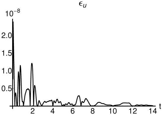
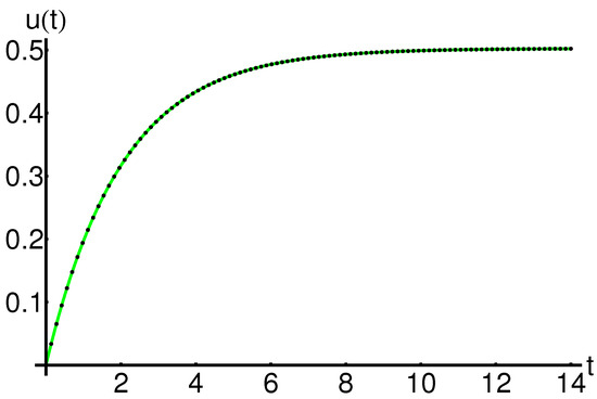
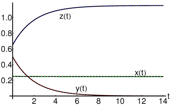
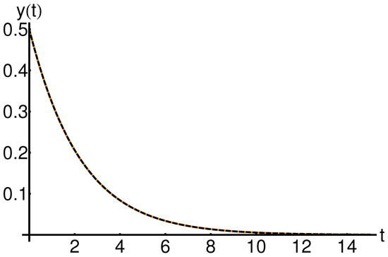
For arbitrary values of the initial conditions $x_0=0.25$, $y_0=0.5$, and $z_0=0.65$, the variations of the approximate analytic solutions ${\overline{u}}_{OHAM}$, ${\overline{x}}_{OHAM}$, ${\overline{y}}_{OHAM}$ and ${\overline{z}}_{OHAM}$ are displayed in Figure 2 and Figure 3, highlighting the accuracy of the analytical procedure.

Figure 2. Variation of the approximate analytic solution ${\overline{u}}_{OHAM}$ of the Equation (6) obtained from Equations (25) and (A1) for the initial conditions $x_0=0.25$, $y_0=0.5$, and $z_0=0.65$ and physical parameters $a=0.01$ and $b=0.5$: OHAM solution (dotted black line) and numerical solution (solid color line), respectively.

Figure 3. Variation of the closed-form solutions ${\overline{x}}_{OHAM}$, ${\overline{y}}_{OHAM}$, ${\overline{z}}_{OHAM}$ given by Equations (7) and (A1) for the initial conditions $x_0=0.25$, $y_0=0.5$, and $z_0=0.65$ and physical parameters $a=0.01$ and $b=0.5$: OHAM solution (dotted black line) and numerical solution (solid color line), respectively.

The semi-analytic closed-form solutions ${\overline{u}}_{OHAM}$ and their corresponding numerical solutions are shown in Table 2, Table 3 and Table 4 for different values of the parameter a and Figure 2.

Table 2. Absolute values of the difference between semi-analytical and numerical solutions: ${ϵ}_u=|u_{numerical}-{\overline{u}}_{OHAM}|$ and the approximate analytic/numerical solution ${\overline{u}}_{OHAM}$ of the Equation (6) given by Equation (25) for the initial conditions $x_0=0.25$, $y_0=0.5$, and $z_0=0.65$ and physical parameters $a=0.25$ and $b=0.5$, respectively.

t	${\mathit{u}}_{\mathit{numerical}}$	${\overline{\mathit{u}}}_{\mathit{OHAM}}$	${\mathit{ϵ}}_{\mathit{u}}$
0	0	0	0
1.4	0.2612420403	0.2612420382	2.1785 · ${10}^{-9}$
2.8	0.4014415549	0.4014415539	1.0805 · ${10}^{-9}$
4.2	0.4762594726	0.4762594725	9.4406 · ${10}^{-11}$
5.6	0.5160735197	0.5160735188	8.5235 · ${10}^{-10}$
7	0.5372295409	0.5372295420	1.0649 · ${10}^{-9}$
8.4	0.5484626729	0.5484626705	2.4558 · ${10}^{-9}$
9.8	0.5544246903	0.5544246900	2.1209 · ${10}^{-10}$
11.2	0.5575883868	0.5575883859	8.8151 · ${10}^{-10}$
12.6	0.5592669866	0.5592669873	6.7086 · ${10}^{-10}$
14	0.5601575693	0.5601575700	6.5030 · ${10}^{-10}$

Table 3. Absolute values of the difference between semi-analytical and numerical solutions: ${ϵ}_u=|u_{numerical}-{\overline{u}}_{OHAM}|$ and the approximate analytic/numerical solution ${\overline{u}}_{OHAM}$ of the Equation (6) given by Equation (25) for the initial conditions $x_0=0.25$, $y_0=0.5$, and $z_0=0.65$ and physical parameters $a=0.5$ and $b=0.5$, respectively.

t	${\mathit{u}}_{\mathit{numerical}}$	${\overline{\mathit{u}}}_{\mathit{OHAM}}$	${\mathit{ϵ}}_{\mathit{u}}$
0	0	0	0
1.4	0.2703163697	0.2703163688	9.2971 · ${10}^{-10}$
2.8	0.4242086592	0.4242086585	6.5222 · ${10}^{-10}$
4.2	0.5100229101	0.5100229099	1.8519 · ${10}^{-10}$
5.6	0.5573923070	0.5573923069	1.1543 · ${10}^{-10}$
7	0.5834044520	0.5834044518	2.0025 · ${10}^{-10}$
8.4	0.5976494461	0.5976494469	8.1155 · ${10}^{-10}$
9.8	0.6054389482	0.6054389477	4.9784 · ${10}^{-10}$
11.2	0.6096950452	0.6096950476	2.4606 · ${10}^{-9}$
12.6	0.6120195336	0.6120195338	2.3045 · ${10}^{-10}$
14	0.6132887639	0.6132887643	3.3906 · ${10}^{-10}$

Table 4. Absolute values of the difference between semi-analytical and numerical solutions: ${ϵ}_u=|u_{numerical}-{\overline{u}}_{OHAM}|$ and the approximate analytic/numerical solution ${\overline{u}}_{OHAM}$ of the Equation (6) given by Equation (25) for the initial conditions $x_0=0.25$, $y_0=0.5$, and $z_0=0.65$ and physical parameters $a=1.5$ and $b=0.5$, respectively.

t	${\mathit{u}}_{\mathit{numerical}}$	${\overline{\mathit{u}}}_{\mathit{OHAM}}$	${\mathit{ϵ}}_{\mathit{u}}$
0	0	0	0
1.4	0.3010382211	0.3010382219	7.8059 · ${10}^{-10}$
2.8	0.4903432586	0.4903432618	3.2032 · ${10}^{-9}$
4.2	0.5971611021	0.5971611019	2.5910 · ${10}^{-10}$
5.6	0.6552077786	0.6552077788	2.0147 · ${10}^{-10}$
7	0.6862665421	0.6862665419	1.5364 · ${10}^{-10}$
8.4	0.7027669743	0.7027669745	2.4074 · ${10}^{-10}$
9.8	0.7115024925	0.7115024920	4.7414 · ${10}^{-10}$
11.2	0.7161189825	0.7161189823	1.9304 · ${10}^{-10}$
12.6	0.7185564406	0.7185564419	1.3568 · ${10}^{-9}$
14	0.7198427802	0.7198427799	2.9513 · ${10}^{-10}$

Comparisons between the semi-analytic closed-form solutions ${\overline{x}}_{OHAM}$ and their corresponding numerical solutions are presented in Table 5, Table 6 and Table 7 for $x_0=0.25$, $y_0=0.5$, and $z_0=0.65$ and physical parameters $a=0.01$ and $b=0.5$, respectively, and Figure 3.

Table 5. Absolute values of the difference between semi-analytical and numerical solutions: ${ϵ}_x=|x_{numerical}-{\overline{x}}_{OHAM}|$ and the approximate analytic/numerical solution ${\overline{x}}_{OHAM}$ given by Equation (7) for the initial conditions $x_0=0.25$, $y_0=0.5$, and $z_0=0.65$ and physical parameters $a=0.01$ and $b=0.5$, respectively.

t	${\mathit{x}}_{\mathit{numerical}}$	${\overline{\mathit{x}}}_{\mathit{OHAM}}$	${\mathit{ϵ}}_{\mathit{x}}$
0	0.25	0.25	0
1.4	0.2487426894	0.2487426896	1.2348 · ${10}^{-10}$
2.8	0.2481185107	0.2481185112	5.5494 · ${10}^{-10}$
4.2	0.2478080592	0.2478080596	4.1476 · ${10}^{-10}$
5.6	0.2476535030	0.2476535031	8.0883 · ${10}^{-11}$
7	0.2475765217	0.2475765220	2.7246 · ${10}^{-10}$
8.4	0.2475381705	0.2475381706	6.0962 · ${10}^{-11}$
9.8	0.2475190618	0.2475190619	7.9550 · ${10}^{-11}$
11.2	0.2475095404	0.2475095404	2.6310 · ${10}^{-11}$
12.6	0.2475047959	0.2475047959	4.6679 · ${10}^{-11}$
14	0.2475024317	0.2475024317	2.6396 · ${10}^{-11}$

Table 6. Absolute values of the difference between semi-analytical and numerical solutions: ${ϵ}_y=|y_{numerical}-{\overline{y}}_{OHAM}|$ and the approximate analytic/numerical solutions ${\overline{y}}_{OHAM}$ given by Equation (7) for the initial conditions $x_0=0.25$, $y_0=0.5$, and $z_0=0.65$ and physical parameters $a=0.01$ and $b=0.5$, respectively.

t	${\mathit{y}}_{\mathit{numerical}}$	${\overline{\mathit{y}}}_{\mathit{OHAM}}$	${\mathit{ϵ}}_{\mathit{y}}$
0	0.5	0.5	0
1.4	0.2491607489	0.2491607498	8.7785 · ${10}^{-10}$
2.8	0.1241604891	0.1241606103	1.2121 · ${10}^{-7}$
4.2	0.0618706396	0.0618707313	9.1618 · ${10}^{-8}$
5.6	0.0308308092	0.0308308314	2.2159 · ${10}^{-8}$
7	0.0153632479	0.0153632924	4.4559 · ${10}^{-8}$
8.4	0.0076556690	0.0076556753	6.2894 · ${10}^{-9}$
9.8	0.0038148819	0.0038148952	1.3269 · ${10}^{-8}$
11.2	0.0019009940	0.0019009970	2.9958 · ${10}^{-9}$
12.6	0.0009472768	0.0009472838	6.9959 · ${10}^{-9}$
14	0.0004720372	0.0004720397	2.5038 · ${10}^{-9}$

Table 7. Absolute values of the difference between semi-analytical and numerical solutions: ${ϵ}_z=|z_{numerical}-{\overline{z}}_{OHAM}|$ and the approximate analytic/numerical solution ${\overline{z}}_{OHAM}$ given by Equation (7) for the initial conditions $x_0=0.25$, $y_0=0.5$, and $z_0=0.65$ and physical parameters $a=0.01$ and $b=0.5$, respectively.

t	${\mathit{z}}_{\mathit{numerical}}$	${\overline{\mathit{z}}}_{\mathit{OHAM}}$	${\mathit{ϵ}}_{\mathit{z}}$
0	0.65	0.65	0
1.4	0.9020965615	0.9020965367	2.4823 · ${10}^{-8}$
2.8	1.0277210001	1.0277208918	1.0828 · ${10}^{-7}$
4.2	1.0903213010	1.0903212213	7.9741 · ${10}^{-8}$
5.6	1.1215156876	1.1215156753	1.2301 · ${10}^{-8}$
7	1.1370602302	1.1370601790	5.1236 · ${10}^{-8}$
8.4	1.1448061603	1.1448061516	8.7078 · ${10}^{-9}$
9.8	1.1486660562	1.1486660437	1.2484 · ${10}^{-8}$
11.2	1.1505894654	1.1505894637	1.7411 · ${10}^{-9}$
12.6	1.1515479272	1.1515479213	5.8597 · ${10}^{-9}$
14	1.1520255310	1.1520255292	1.7628 · ${10}^{-9}$

The variations of the approximate analytic solution ${\overline{u}}_{OHAM}$ and each of ${\overline{x}}_{OHAM}$, ${\overline{y}}_{OHAM}$ and ${\overline{z}}_{OHAM}$ have an asymptotic behavior as displayed in Figure 2 and Figure 3.

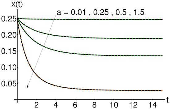
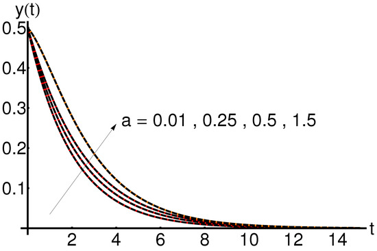
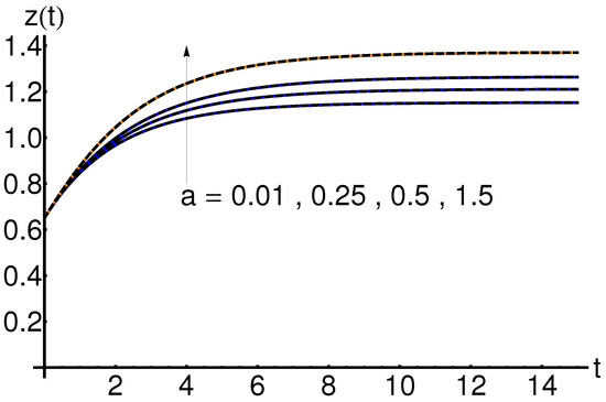
5.1. Effect of the Parameter a

The effect of the parameter a on the system states $x\left(t\right)$, $y\left(t\right)$ and $z\left(t\right)$ is shown in Figure 4, Figure 5 and Figure 6. An increase in the infection rate a leads to an increase in the functions ${\overline{y}}_{OHAM}$ and ${\overline{z}}_{OHAM}$ respectively, while the function ${\overline{x}}_{OHAM}$ slowly decreases with time.

Figure 4. Influence of the parameter a on the closed-form solutions ${\overline{x}}_{OHAM}$ given by Equations (7) and (A1)–(A4) for the initial conditions $x_0=0.25$, $y_0=0.5$, and $z_0=0.65$ and physical parameter $b=0.5$: OHAM solution (dotted black line) and numerical solution (solid color line), respectively.

Figure 5. Influence of the parameter a on the closed-form solutions ${\overline{y}}_{OHAM}$ given by Equations (7) and (A1)–(A4) for the initial conditions $x_0=0.25$, $y_0=0.5$, and $z_0=0.65$ and physical parameter $b=0.5$: OHAM solution (dotted black line) and numerical solution (solid color line), respectively.

Figure 6. Influence of the parameter a on the closed-form solutions ${\overline{z}}_{OHAM}$ given by Equations (7) and (A1)–(A4) for the initial conditions $x_0=0.25$, $y_0=0.5$, and $z_0=0.65$ and physical parameter $b=0.5$: OHAM solution (dotted black line) and numerical solution (solid color line), respectively.

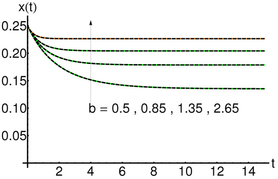
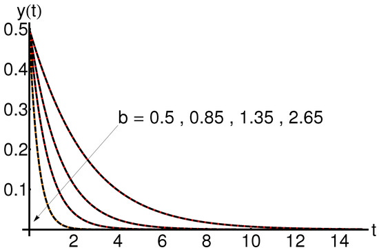
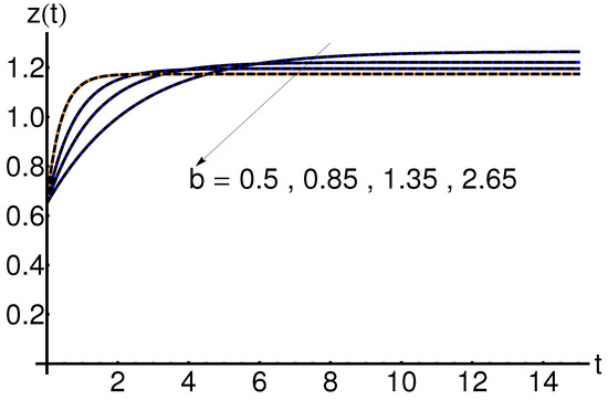
5.2. Effect of the Parameter b

The effect of the parameter b on the system states $x\left(t\right)$, $y\left(t\right)$ and $z\left(t\right)$ is shown in Figure 7, Figure 8 and Figure 9. An increase in the removal rate of the infected subjects b leads to an increase in the function ${\overline{x}}_{OHAM}$ and a decrease in the function ${\overline{y}}_{OHAM}$, respectively, while the variation of the function ${\overline{z}}_{OHAM}$ is determined by the value of the infection rate a.

Figure 7. Influence of the parameter b on the closed-form solutions ${\overline{x}}_{OHAM}$ given by Equations (7), (A3) and (A5)–(A7) for the initial conditions $x_0=0.25$, $y_0=0.5$, and $z_0=0.65$ and physical parameter $a=0.5$: OHAM solution (dotted black line) and numerical solution (solid color line), respectively.

Figure 8. Influence of the parameter b on the closed-form solutions ${\overline{y}}_{OHAM}$ given by Equations (7), (A3) and (A5)–(A7) for the initial conditions $x_0=0.25$, $y_0=0.5$, and $z_0=0.65$ and physical parameter $a=0.5$: OHAM solution (dotted black line) and numerical solution (solid color line), respectively.

Figure 9. Influence of the parameter b on the closed-form solutions ${\overline{z}}_{OHAM}$ given by Equations (7), (A3) and (A5)–(A7) for the initial conditions $x_0=0.25$, $y_0=0.5$, and $z_0=0.65$ and physical parameter $a=0.5$: OHAM solution (dotted black line) and numerical solution (solid color line), respectively.

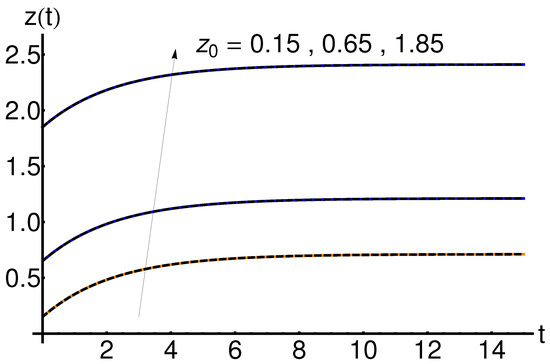
5.3. Effect of the Initial Condition $x_0$

The effect of the initial condition $x_0$ on the system states $x\left(t\right)$, $y\left(t\right)$, and $z\left(t\right)$ is shown in Figure 10, Figure 11 and Figure 12. An increase in the initial condition $x_0$ leads to an increase in the functions ${\overline{x}}_{OHAM}$, ${\overline{y}}_{OHAM}$, and ${\overline{z}}_{OHAM}$, respectively, for fixed values of the physical parameters a and b.

Figure 10. Influence of the initial condition $x_0$ on the closed-form solutions ${\overline{x}}_{OHAM}$ given by Equations (7), (A3) and (A8)–(A10) for the initial conditions $y_0=0.5$ and $z_0=0.65$ and physical parameters $a=0.5$ and $b=0.5$: OHAM solution (dotted black line) and numerical solution (solid color line), respectively.

Figure 11. Influence of the initial condition $x_0$ on the closed-form solutions ${\overline{y}}_{OHAM}$ given by Equations (7), (A3) and (A8)–(A10) for the initial conditions $y_0=0.5$ and $z_0=0.65$ and physical parameters $a=0.5$ and $b=0.5$: OHAM solution (dotted black line) and numerical solution (solid color line), respectively.

Figure 12. Influence of the initial condition $x_0$ on the closed-form solutions ${\overline{z}}_{OHAM}$ given by Equations (7), (A3) and (A8)–(A10) for the initial conditions $y_0=0.5$ and $z_0=0.65$ and physical parameters $a=0.5$ and $b=0.5$: OHAM solution (dotted black line) and numerical solution (solid color line), respectively.

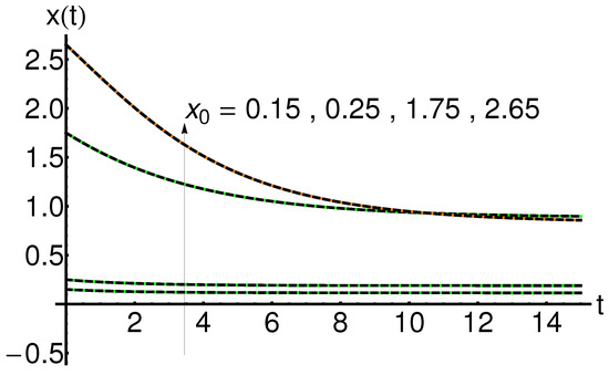
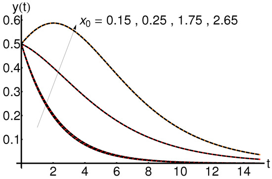
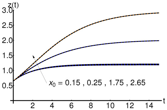
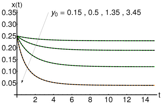
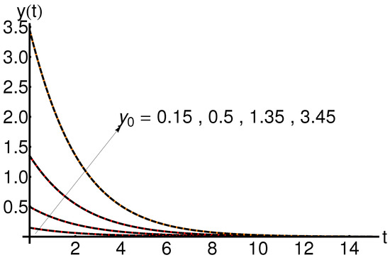
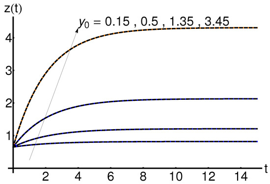
5.4. Effect of the Initial Condition $y_0$

The effect of the initial condition $y_0$ on the system states $x\left(t\right)$, $y\left(t\right)$, and $z\left(t\right)$ is shown in Figure 13, Figure 14 and Figure 15. An increase in the initial condition $y_0$ leads to an increase in the functions ${\overline{y}}_{OHAM}$, ${\overline{z}}_{OHAM}$ respectively, while the function ${\overline{x}}_{OHAM}$ decreases with time, for fixed values of the physical parameters a and b.

Figure 13. Influence of the initial condition $y_0$ on the closed-form solutions ${\overline{x}}_{OHAM}$ given by Equations (7), (A3) and (A11)–(A13) for the initial conditions $x_0=0.25$ and $z_0=0.65$ and physical parameters $a=0.5$ and $b=0.5$: OHAM solution (dotted black line) and numerical solution (solid color line), respectively.

Figure 14. Influence of the initial condition $y_0$ on the closed-form solutions ${\overline{y}}_{OHAM}$ given by Equations (7), (A3) and (A11)–(A13) for the initial conditions $x_0=0.25$ and $z_0=0.65$ and physical parameters $a=0.5$ and $b=0.5$: OHAM solution (dotted black line) and numerical solution (solid color line), respectively.

Figure 15. Influence of the initial condition $y_0$ on the closed-form solutions ${\overline{z}}_{OHAM}$ given by Equations (7), (A3) and (A11)–(A13) for the initial conditions $x_0=0.25$ and $z_0=0.65$ and physical parameters $a=0.5$ and $b=0.5$: OHAM solution (dotted black line) and numerical solution (solid color line), respectively.

5.5. Effect of the Initial Condition $z_0$

The effect of the initial condition $z_0$ on the system states $x\left(t\right)$, $y\left(t\right)$ and $z\left(t\right)$ is shown in Figure 16, Figure 17 and Figure 18. An increase in the initial condition $y_0$ leads to an increase in the function ${\overline{z}}_{OHAM}$, while the functions ${\overline{x}}_{OHAM}$ and ${\overline{y}}_{OHAM}$, respectively, are not influenced for fixed values of the physical parameters a and b.

Figure 16. Influence of the initial condition $z_0$=$0.15,0.65,1.85$ on the closed-form solutions ${\overline{x}}_{OHAM}$ given by Equations (7), (A3), (A14) and (A15) for the initial conditions $x_0=0.25$ and $y_0=0.5$ and physical parameters $a=0.5$ and $b=0.5$: OHAM solution (dotted black line) and numerical solution (solid color line), respectively.

Figure 17. Influence of the initial condition $z_0$=$0.15,0.65,1.85$ on the closed-form solutions ${\overline{y}}_{OHAM}$ given by Equations (7), (A3), (A14) and (A15) for the initial conditions $x_0=0.25$ and $y_0=0.5$ and physical parameters $a=0.5$ and $b=0.5$: OHAM solution (dotted black line) and numerical solution (solid color line), respectively.

Figure 18. Influence of the initial condition $z_0$ on the closed-form solutions ${\overline{z}}_{OHAM}$ given by Equations (7), (A3), (A14) and (A15) for the initial conditions $x_0=0.25$ and $y_0=0.5$ and physical parameters $a=0.5$ and $b=0.5$: OHAM solution (dotted black line) and numerical solution (solid color line), respectively.

5.6. OHAM Solutions versus Iterative Solutions

The OHAM solutions are validation by comparison with the corresponding iterative solutions using the iterative method [25].

Integration of the system (1) over the interval $[0,t]$ yields:

$$\begin{array}{c}{\displaystyle x\left(t\right)=x\left(0\right)+\underset{0}{\overset{t}{\int }}\left(-ax\left(s\right)y\left(s\right)\right)ds}\hfill \\ {\displaystyle y\left(t\right)=y\left(0\right)+\underset{0}{\overset{t}{\int }}\left(ax\left(s\right)y\left(s\right)-by\left(s\right)\right)ds}\hfill \\ {\displaystyle z\left(t\right)=z\left(0\right)+\underset{0}{\overset{t}{\int }}by\left(s\right)ds}\hfill \end{array}.$$

(26)

The iterative algorithm leads to:

$$\begin{array}{c}{\displaystyle x_0\left(t\right)=x\left(0\right),x_1\left(t\right)=N_1(x_0,y_0,z_0)=\underset{0}{\overset{t}{\int }}\left(-a{x}_0\left(s\right)y_0\left(s\right)\right)ds,}\hfill \\ {\displaystyle y_0\left(t\right)=y\left(0\right),y_1\left(t\right)=N_2(x_0,y_0,z_0)=\underset{0}{\overset{t}{\int }}\left(a{x}_0\left(s\right)y_0\left(s\right)-b{y}_0\left(s\right)\right)ds,}\hfill \\ {\displaystyle z_0\left(t\right)=z\left(0\right),z_1\left(t\right)=N_3(x_0,y_0,z_0)=\underset{0}{\overset{t}{\int }}b{y}_0\left(s\right)ds,}\hfill \\ \cdots \hfill \\ x_m\left(t\right)=N_1\left({\displaystyle \sum _{i=0}^{m-1}{x}_i,\sum _{i=0}^{m-1}{y}_i,\sum _{i=0}^{m-1}{z}_i}\right)-N_1\left({\displaystyle \sum _{i=0}^{m-2}{x}_i,\sum _{i=0}^{m-2}{y}_i,\sum _{i=0}^{m-2}{z}_i}\right),\hfill \\ y_m\left(t\right)=N_2\left({\displaystyle \sum _{i=0}^{m-1}{x}_i,\sum _{i=0}^{m-1}{y}_i,\sum _{i=0}^{m-1}{z}_i}\right)-N_2\left({\displaystyle \sum _{i=0}^{m-2}{x}_i,\sum _{i=0}^{m-2}{y}_i,\sum _{i=0}^{m-2}{z}_i}\right),\hfill \\ z_m\left(t\right)=N_3\left({\displaystyle \sum _{i=0}^{m-1}{x}_i,\sum _{i=0}^{m-1}{y}_i,\sum _{i=0}^{m-1}{z}_i}\right)-N_3\left({\displaystyle \sum _{i=0}^{m-2}{x}_i,\sum _{i=0}^{m-2}{y}_i,\sum _{i=0}^{m-2}{z}_i}\right),\hfill \\ m\ge 2.\hfill \end{array}$$

(27)

The solutions of Equation (1), using the iterative algorithm, can be written as:

$${\displaystyle x_{iter}\left(t\right)=\sum _{m=0}^{\infty }{x}_m\left(t\right),y_{iter}\left(t\right)=\sum _{m=0}^{\infty }{y}_m\left(t\right),z_{iter}\left(t\right)=\sum _{m=0}^{\infty }{z}_m\left(t\right),}$$

The iterative solutions $x_{iter}\left(t\right)$, after 6 iterations and considering the initial conditions $x\left(0\right)=2.65$, $y\left(0\right)=0.5$, and $z\left(0\right)=0.65$ (presented in Table 8), taking into account algorithm (27), become:

$$\begin{array}{c}{\displaystyle x_{iter}\left(t\right)=\sum _{m=0}^6{x}_m\left(t\right)=2.65-0.33125t-0.0062109374t^2+0.0056157226t^3+}\hfill \\ +0.0001049443t^4-0.0001240799t^5-1.482662·{10}^{-6}{t}^6+2.855943·{10}^{-6}{t}^7+\hfill \\ +6.846024·{10}^{-9}{t}^8-6.412486·{10}^{-8}{t}^9+8.825498·{10}^{-10}{t}^{10}+\hfill \\ +1.314505·{10}^{-9}{t}^{11}+\mathcal{O}\left({10}^{-11}\right)\hfill \\ \\ {\displaystyle y_{iter}\left(t\right)=\sum _{m=0}^6{y}_m\left(t\right)=0.5+0.0812499999t-0.0141015625t^2-0.0032654622t^3+}\hfill \\ +0.0003032384t^4+0.0000937561t^5-6.330349·{10}^{-6}{t}^6-2.411638·{10}^{-6}{t}^7+\hfill \\ +1.353642·{10}^{-7}{t}^8+5.707997·{10}^{-8}{t}^9-3.044148·{10}^{-9}{t}^{10}-\hfill \\ -1.209882·{10}^{-9}{t}^{11}+\mathcal{O}\left({10}^{-11}\right)\hfill \\ \\ {\displaystyle z_{iter}\left(t\right)=\sum _{m=0}^6{z}_m\left(t\right)=0.65+0.25t+0.0203124999t^2-0.0023502604t^3-}\hfill \\ -0.0004081827t^4+0.0000303238t^5+7.813012·{10}^{-6}{t}^6-4.443055·{10}^{-7}{t}^7-\hfill \\ -1.422102·{10}^{-7}{t}^8+7.044892·{10}^{-9}{t}^9+2.161598·{10}^{-9}{t}^{10}-\hfill \\ -1.046225·{10}^{-10}{t}^{11}+\mathcal{O}\left({10}^{-11}\right).\hfill \end{array}$$

(28)

Table 8. Values of the approximate analytical solution ${\overline{x}}_{OHAM}\left(t\right)$ (A10), the iterative solution $x_{iter}\left(t\right)$ Equation (28) and the corresponding numerical solution.

t	${\mathit{x}}_{\mathit{numerical}}$	${\overline{\mathit{x}}}_{\mathit{OHAM}}$	${\mathit{x}}_{\mathit{iter}}$
0	2.65	2.65	2.65
4/5	2.3839027541	2.3839029712	2.3839027796
8/5	2.1265371138	2.1265365783	2.1265366737
12/5	1.8913510362	1.8913513920	1.8913455854
16/5	1.6863059873	1.6863056711	1.6862867053
4	1.5138975803	1.5138971816	1.5138965974
24/5	1.3726607934	1.3726608378	1.3728898569
28/5	1.2589780741	1.2589782405	1.2600385486
32/5	1.1684877088	1.1684876850	1.1715506355
36/5	1.0969288554	1.0969286855	1.1037806698
8	1.0405377496	1.0405375783	1.0534780923
44/5	0.9961676597	0.9961676512	1.0178983901
48/5	0.9612691958	0.9612693104	0.9952158376
52/5	0.9338130529	0.9338131801	0.9866939239
56/5	0.9121993795	0.9121994313	1.0082617489
12	0.8951728310	0.8951727843	1.1713190209

The precision and efficiency of the OHAM method (using just one iteration) compared to the iterative method described in [25] (using six iterations) are represented in Table 8 and Figure 19, Figure 20 and Figure 21, respectively, highlighting the accuracy and efficiency of the OHAM technique (using just one iteration) by comparison with the iterative method described in [25] (using six iterations).

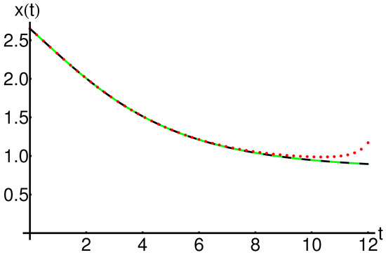
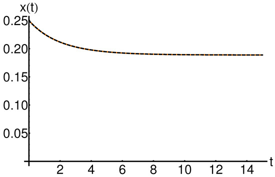
Figure 19. Profile of the approximate analytical solution ${\overline{x}}_{OHAM}\left(t\right)$ of Equation (1) given by Equation (A10), the iterative solution $x_{iter}\left(t\right)$ given by Equation (28) and the corresponding numerical solution: OHAM solution (dashing black line), iterative solution (dotted red line) and numerical solution (solid color line), respectively.

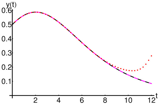
Figure 20. Profile of the approximate analytical solution ${\overline{y}}_{OHAM}\left(t\right)$ of Equation (1) given by Equation (A10), the iterative solution $y_{iter}\left(t\right)$ given by Equation (28) and the corresponding numerical solution: OHAM solution (dashing black line), iterative solution (dotted red line) and numerical solution (solid color line), respectively.

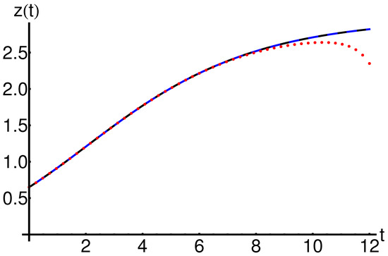
Figure 21. Profile of the approximate analytical solution ${\overline{z}}_{OHAM}\left(t\right)$ of Equation (1) given by Equation (A10), the iterative solution $z_{iter}\left(t\right)$ given by Equation (28) and the corresponding numerical solution: OHAM solution (dashing black line), iterative solution (dotted red line) and numerical solution (solid color line), respectively.

Figure 19, Figure 20 and Figure 21 and Table 8, respectively, present a parallel between the OHAM solutions ${\overline{x}}_{OHAM}$, ${\overline{y}}_{OHAM}$, ${\overline{z}}_{OHAM}$ and the corresponding iterative solutions $x_{iter}$ given in Equation (28).

The semi-analytical solutions ${\overline{u}}_{OHAM}$ for different values of the initial conditions $x_0$, $y_0$, and $z_0$ and different values of the physical parameters a and b are presented in detail in Appendix A.

5.7. OHAM Solutions versus Exact Parametric Solutions

Harko et al. [3] established the exact parametric solution of Equation (1) as:

$$\begin{array}{c}{\displaystyle x\left(t\right)=X_{0}v\left(t\right)}\hfill \\ {\displaystyle y\left(t\right)=\frac{b}{a}ln\left(v\left(t\right)\right)-X_{0}v\left(t\right)-\frac{P_1}{a}}\hfill \\ {\displaystyle z\left(t\right)=-\frac{b}{a}ln\left(v\left(t\right)\right)}\hfill \end{array},$$

(29)

where the unknown smooth function $v\left(t\right)$ (as parameter) is a solution of the nonlinear second-order differential equation:

$$\left\{\begin{array}{c}{\displaystyle v\frac{d^{2}v}{d{t}^2}-{\left(\frac{dv}{dt}\right)}^2+\left(b-X_{0}av\right)v\frac{dv}{dt}=0}\hfill \\ {\displaystyle v\left(0\right)=v_0=e^{-\frac{a}{b}{N}_3},\frac{dv}{dt}\left(0\right)=-a{N}_2{e}^{-\frac{a}{b}{N}_3}}\hfill \end{array}.\right.$$

(30)

The exact solution of the above Equation (30) in explicit form remains an open problem and could be just analytically solved by different analytical methods.

The implicit solution of Equation (30) in integral representation form is:

$$\begin{array}{c}{\displaystyle t-t_0={\int }_{v_0}^v\frac{d\xi }{\xi \left(P_1-bln\left(\xi \right)+X_{0}a\xi \right)}}\hfill \end{array},$$

(31)

with $x\left(0\right)=N_1$, $y\left(0\right)=N_2$, $z\left(0\right)=N_3$, $N=N_1+N_2+N_3$, $P_1=-aN$, and $X_0=N_1{e}^{\frac{a}{b}{N}_3}$.

A comparison between the OHAM solution with the exact parametric solution [3] is shown in Figure 22.

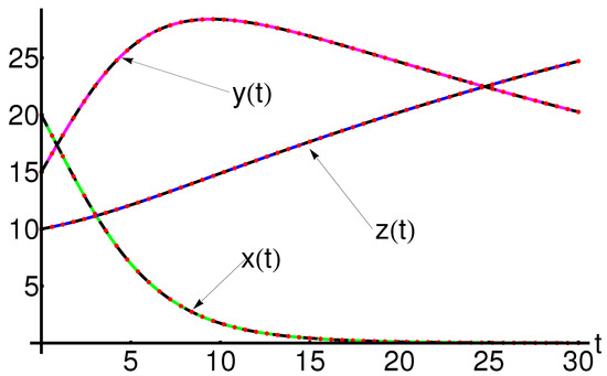
Figure 22. Comparison between the closed-form solutions ${\overline{x}}_{OHAM}$, ${\overline{y}}_{OHAM}$, ${\overline{z}}_{OHAM}$ given by Equations (7) and (A16), exact parametric solutions given by Equations (29) and (30) and corresponding numerical solutions, respectively, for initial conditions $x_0=N_1=20$, $y_0=N_2=15$, and $z_0=N_3=10$ and physical parameters $a=0.01$ and $b=0.02$: OHAM solution (dashing black line), exact parametric solution (dotted red line) and numerical solution (solid color line), respectively.

6. Conclusions

An analytical approach, namely OHAM, for solving second-order nonlinear differential equations is adopted using only one iteration. The analytical approximate solutions represent the $\epsilon$-approximate OHAM solutions.

Advantages of this analytical method are reflected by comparison between the analytical solutions, numerical results (via the fourth-order Runge–Kutta method) and corresponding iterative solutions (via a known iterative method).

The obtained results are validated by graphically comparing them with the corresponding numerical solutions and by numerical integral values of the square residuals. The corresponding absolute values of the difference between semi-analytical and numerical solutions are tabulated. These comparisons prove the precision of the applied method in the sense that the analytical solutions are approaching the exact solution. The obtained results are in a good agreement with the exact parametric solutions and corresponding numerical results.

The achieved results encourage the study of dynamical systems with similar properties, as epidemic approach to equilibrium, for the future work.

References

- Brauer, F. The Kermack-McKendrick epidemic model revisited. Math. Biosci. 2005, 198, 119–131. [Google Scholar] [CrossRef] [PubMed]
- Harko, T.; Mak, M.K. A simple computational approach to the Susceptible-Infected-Recovered (SIR) epidemic model via the Laplace-Adomian Decomposition Method. Rom. Rep. Phys. 2021, 73, 11. [Google Scholar]
- Harko, T.; Lobo, F.S.N.; Mak, M.K. Exact analytical solutions of the Susceptible-Infected-Recovered (SIR) epidemic model and of the SIR model with equal death and birth rates. Appl. Math. Comput. 2014, 236, 184–194. [Google Scholar] [CrossRef]
- Semendyaeva, N.L.; Orlov, M.V.; Rui, T.; Enping, Y. Analytical and numerical investigation of the SIR mathematical model. Comput. Math. Model. 2022, 33, 284–299. [Google Scholar] [CrossRef]
- Prodanov, D. Computational aspects of the approximate analytic solutions of the SIR model: Applications to modelling of COVID-19 outbreaks. Nonlinear Dynam. 2023, 111, 15613–15631. [Google Scholar] [CrossRef]
- Pakes, A.G. A SIR Epidemic Model Allowing Recovery. Axioms 2024, 13, 115. [Google Scholar] [CrossRef]
- MacFarlane, A.I. Dynamic structure theory: A structural approach to social and biological systems. Bull. Math. Biol. 1981, 43, 579–591. [Google Scholar] [CrossRef]
- Motee, N.; Bamieh, B.; Khammash, M. Stability analysis of quasi-polynomial dynamical systems with applications to biological network models. Automatica 2012, 48, 2945–2950. [Google Scholar] [CrossRef]
- Toledo-Hernandez, R.; Rico-Ramirez, V.; Rico-Martinez, R.; Hernandez-Castro, S.; Diwekar, U.M. A fractional calculus approach to the dynamic optimization of biological reactive systems. Part II: Numerical solution of fractional optimal control problems. Chem. Eng. Sci. 2014, 117, 239–247. [Google Scholar] [CrossRef]
- Toledo-Hernandez, R.; Rico-Ramirez, V.; Rico-Martinez, R.; Hernandez-Castro, S.; Diwekar, U.M. A fractional calculus approach to the dynamic optimization of biological reactive systems. Part I: Fractional models for biological reactions. Chem. Eng. Sci. 2014, 117, 217–228. [Google Scholar] [CrossRef]
- Figueiredo, D.; Martins, M.A.; Chaves, M. Applying differential dynamic logic to reconfigurable biological networks. Math. Biosci. 2017, 291, 10–20. [Google Scholar] [CrossRef] [PubMed]
- Liu, X.; Tong, X.; Zhang, M.; Wang, Z. A highly secure image encryption algorithm based on conservative hyperchaotic system and dynamic biogenetic gene algorithms. Chaos Solitons Fract. 2023, 171, 113450. [Google Scholar] [CrossRef]
- Cheung, N.J.; Xu, Z.-K.; Ding, X.-M.; Shen, H.-B. Modeling nonlinear dynamic biological systems with human–readable fuzzy rules optimized by convergent heterogeneous particle swarm. Eur. J. Oper. Res. 2015, 247, 349–358. [Google Scholar] [CrossRef]
- Daun, S.; Rubin, J.; Vodovotz, Y.; Clermont, G. Equation-based models of dynamic biological systems. J. Crit. Care 2008, 23, 585–594. [Google Scholar] [CrossRef] [PubMed]
- Malchow, H. Dynamical Stabilization of an Unstable Equilibrium in Chemical and Biological Systems. Math. Comput. Model. 2002, 36, 307–319. [Google Scholar] [CrossRef]
- Liu, F.; Burrage, K. Novel techniques in parameter estimation for fractional dynamical models arising from biological systems. Comput. Math. Appl. 2011, 62, 822–833. [Google Scholar] [CrossRef]
- Gulati, P.; Chauhan, S.; Mubayi, A.; Singh, T.; Rana, P. Dynamical analysis, optimum control and pattern formation in the biological pest (EFSB) control model. Chaos Solitons Fract. 2021, 147, 110920. [Google Scholar] [CrossRef]
- Al-Nassir, S. Dynamic analysis of a harvested fractional-order biological system with its discretization. Chaos Solitons Fract. 2021, 152, 111308. [Google Scholar] [CrossRef]
- Lampartová, A.; Lampart, M. Exploring diverse trajectory patterns in nonlinear dynamic systems. Chaos Solitons Fract. 2024, 182, 114863. [Google Scholar] [CrossRef]
- Francis, O.; Aminer, T.; Okelo, B.; Manyala, J. Dynamical Analysis of Prey Refuge Effects on the Stability of Holling Type III Four-species Predator-Prey System. Results Control Optim. 2024, 14, 100390. [Google Scholar] [CrossRef]
- Kermack, W.O.; McKendrick, A.G. A contribution to the mathematical theory of epidemics. Proc. R. Soc. A Math. 1927, 115, 700–721. [Google Scholar]
- Lazureanu, C.; Binzar, T. Stability and energy-Casimir mapping for integrable deformations of the Kermack-McKendrick system. Adv. Math. Phys. 2018, 2018, 5398768. [Google Scholar] [CrossRef]
- Marinca, V.; Herisanu, N. The Optimal Homotopy Asymptotic Method–Engineering Applications; Springer: Berlin/Heidelberg, Germany, 2015. [Google Scholar]
- Ene, R.D.; Pop, N.; Lapadat, M.; Dungan, L. Approximate closed-form solutions for the Maxwell–Bloch equations via the Optimal Homotopy Asymptotic Method. Mathematics 2022, 10, 4118. [Google Scholar] [CrossRef]
- Daftardar-Gejji, V.; Jafari, H. An iterative method for solving nonlinear functional equations. J. Math. Anal. Appl. 2006, 316, 753–763. [Google Scholar] [CrossRef]
Disclaimer/Publisher’s Note: The statements, opinions and data contained in all publications are solely those of the individual author(s) and contributor(s) and not of MDPI and/or the editor(s). MDPI and/or the editor(s) disclaim responsibility for any injury to people or property resulting from any ideas, methods, instructions or products referred to in the content. |
© 2024 by the authors. Licensee MDPI, Basel, Switzerland. This article is an open access article distributed under the terms and conditions of the Creative Commons Attribution (CC BY) license (https://creativecommons.org/licenses/by/4.0/).