Modeling the Nonmonotonic Immune Response in a Tumor–Immune System Interaction

Abstract

Tumor–immune system interactions are very complicated, being highly nonlinear and not well understood. A large number of tumors can potentially weaken the immune system through various mechanisms such as secreting cytokines that suppress the immune response. In this paper, we propose a tumor–immune system interaction model with a nonmonotonic immune response function and adoptive cellular immunotherapy (ACI). The model has a tumor-free equilibrium and at most three tumor-presence equilibria (low, moderate and high ones). The stability of all equilibria is studied by analyzing their characteristic equations. The consideration of nonmonotonic immune response results in a series of bifurcations such as the saddle-node bifurcation, transcritical bifurcation, Hopf bifurcation and Bogdanov–Takens bifurcation. In addition, numerical simulation results show the coexistence of periodic orbits and homoclinic orbits. Interestingly, along with various bifurcations, we also found two bistable scenarios: the coexistence of a stable tumor-free as well as a high-tumor-presence equilibrium and the coexistence of a stable-low as well as a high-tumor-presence equilibrium, which can show symmetric and antisymmetric properties in a range of model parameters and initial cell concentrations. The new findings indicate that under ACI, patients can possibly reach either a stable tumor-free state or a low-tumor-presence state in the presence of nonmonotonic immune response once the immune system is activated.

1. Introduction

The immune system can recognize and control nascent tumor cells through a process called immunosurveillance [1]. This involves main antitumor immune cells such as dendritic cells, T cells, natural killer (NK) cells and tumor-associated macrophages (TAMs) to identify and eliminate abnormal or cancerous cells [2]. However, tumors can evade attacks from the immune system by various mechanisms, such as restricting antigen recognition, orchestrating an immunosuppressive microenvironment, inducing T cell exhaustion and so on [3,4]. Understanding tumor–immune system interactions is essential for developing effective immunotherapies to treat tumors. Immunotherapy is a transformative strategy that activates the body’s immune response against a tumor [5]. It can include treatments like adoptive cellular immunotherapy (ACI), oncolytic virus therapy, cancer vaccines, immune checkpoint therapy and combination therapies [6,7].

A variety of mathematical models have been proposed and analyzed to explore the dynamics of tumor–immune system interactions and have evolved to capture much more complex aspects of the immune response [8], such as healthy cells [9], natural killer cells [10], helper T cells [11], regulatory T cells [12], macrophages [13] and so on. For mathematical simplicity, a bilinear form has mainly been used to describe the growth of the immune response to tumors [14]. However, tumor–immune system interactions are very complicated, being highly nonlinear, and evolve with time to a certain extent [15]. So it is necessary to model tumor–immune system interactions using nonlinear response functions, which are widely used in the modeling of tumor–immune interactions [16], the ecological system [17], virus dynamics [18], the metabolic system [19] and so on.

Kuznetsov et al. [20] developed a classical model describing the effector cell response to the growth of an immunogenic tumor, where the rate of stimulated accumulation of effector cells attains a maximum value as the number of T cells becomes large. Kirschner et al. [21] introduced cytokine interleukin-2 (IL-2) and ACI into the tumor–immune interaction model with the Michaelis–Menten form to indicate the saturated effects of the immune response. Their model can explain both short-term oscillations in tumor sizes and long-term tumor relapse. Dritschel et al. [22] considered adding a helper T cell compartment to Kuznetsov’s model to distinguish immune cell promotion and tumor cell killing, and they implicitly incorporated tumor-modulated immunosupression by altering the functions describing immune recruitment and proliferation. Their model can exhibit the three phases (elimination, equilibrium and escape) of cancer immunoediting, periodic growth and suppression of the immune and tumor populations. Talkington [23] explored and compared four previous models with adoptive immunotherapy that predict successful tumor elimination. Song et al. [24] developed a tumor growth model with immune system response and drug therapy to study the mechanisms of chemotherapy. Bekker et al. [25] carried out a survey of mathematical models to evaluate the effects of radiotherapy on tumor–immune system interactions. Butner et al. [26] presented a comprehensive review of mathematical models on cancer immunotherapy for clinical applications. Tang et al. [27] developed a mathematical model to investigate the interactions between effector cells, tumor cells and cytokines with pulsed radio/chemo-immunotherapy. Recently, Zhang et al. [28] investigated a tumor–immune system interaction model with saturated activation of T cells and dendritic cell therapy showing rich dynamics.

We investigate the effect of nonlinear interactions between tumor and immune cells in the tumor microenvironment. Inspired by previous studies, we propose the following ordinary differential equations model with nonlinear tumor–immune interactions:

$$\left\{\begin{array}{cc}\hfill \frac{dT}{dt}=& aT(1-bT)-\frac{ncET}{T^2+c^2},\hfill \\ \hfill \frac{dE}{dt}=& s_1-d_{1}E+pEH,\hfill \\ \hfill \frac{dH}{dt}=& s_2-d_{2}H+kTH,\hfill \end{array}\right.$$

(1)

where $T\left(t\right)$, $E\left(t\right)$ and $H\left(t\right)$ represent the populations of tumor cells (TCs), effector cells (ECs) and helper T cells (HTCs), respectively. Here, both ECs and HTCs correspond to the immune system/immune response. The growth of TCs is assumed to follow the logistic form $aT(1-bT)$, where a is the maximal growth rate and $b^{-1}$ is the maximal carrying capacity of the biological environment for TCs. In the initial stage, the immune system recognizes tumor antigens, and a large number of immune cells are recruited into the tumor microenvironment. Over time, tumors can generate various mechanisms to escape immune surveillance, such as recruiting immunosuppressive cells like regulatory T cells and secreting immunosuppressive cytokines like IL-6 [29]. Furthermore, the presence of a large number of tumor cells can suppress and weaken the immune system, allowing tumors to evade immune surveillance and continue to grow [30,31]. Therefore, we assume that the inhibition of TCs by ECs follows biphasic dependence on the number of TCs using a nonmonotonic response function $F\left(T\right)=\frac{ncT}{T^2+c^2}$, where $F\left(T\right)$ increases first to the peak and then decreases to zero as T is sufficiently large [32]. n represents the maximal inhibition rate of TCs by ECs, and c is the number of TCs at which ECs’ inhibition is half-maximal. The inhibition rate of ECs on TCs attains a maximum value of $n/2$ when $T=c$ and decays to zero as $T\to +\infty$. Here, we consider a weak proliferation of ECs stimulating TCs as $pEH$, while ignoring the ECs’ stimulation from TCs [33]. p is the activation rate of ECs by HTCs, and k is the HTCs’ stimulation rate by the presence of identified tumor antigens. $s_1$ refers to the constant inflow of ACI, and $s_2$ is the birth rate of HTCs produced in the bone marrow. $d_1$ and $d_2$ are the natural death rates of ECs and HTCs, respectively. All model parameters are positive and described in Table 1.

Table 1. Model parameters.

Parameter	Description	Reference
a	Proliferation rate of TCs	[20]
$b^{-1}$	Carrying capacity of TCs	[20]
n	Maximal inhibition rate of TCs by ECs	[20]
c	Half-velocity constant	[22]
$s_1$	Constant inflow of ACI	[11,22]
$d_1$	Death rate of ECs	[11,22]
p	Activation rate of ECs by HTCs	[11]
$s_2$	Birth rate of HTCs produced in the bone marrow	[11,22]
$d_2$	Death rate of HTCs	[11,22]
k	HTCs’ stimulation rate by identified tumor antigens	[11]

As far as we know, this is the first attempt to model the immune response against a tumor by a nonmonotonic response function, which can capture long-term tumor–immune system interactions. In this study, we aim to exploit the rich dynamics of model (1), with nonmonotonic immune response function and ACI, and explain the biological implications of dynamical properties. The rest of this paper is organized as follows. In Section 2, we firstly nondimensionalize system (1) by scaling the parameters. Then we study the existence and stability of possible equilibria of the dimensionless system. In Section 3, we carry out a bifurcation analysis including saddle-node bifurcation, transcritical bifurcation and Hopf bifurcation. In Section 4, we investigate the effects of some parameters on the stability of each equilibrium and perform the numerical simulations to show several types of bifurcations and bistability phenomena. In the last section, we give a summary and discussion.

2. Stability Analysis

In this section, we firstly nondimensionalize system (1), and then we study the existence and stability of possible equilibria of the dimensionless system.

2.1. Dimensionless Model

The first step is to nondimensionalize system (1). Let

$$\widehat{t}=t{d}_1,x=bT,y=bE,z=\frac{pH}{d_1}.$$

Then we obtain

$$\left\{\begin{array}{cc}\hfill \frac{dx}{d\widehat{t}}=& \widehat{a}x(1-x)-\frac{\widehat{n}xy}{x^2+{\widehat{c}}^2},\hfill \\ \hfill \frac{dy}{d\widehat{t}}=& \widehat{s_1}-y+yz,\hfill \\ \hfill \frac{dz}{d\widehat{t}}=& \widehat{s_2}-\widehat{d_2}z+\widehat{k}xz,\hfill \end{array}\right.$$

(2)

where

$$\widehat{a}=\frac{a}{d_1},\widehat{n}=\frac{ncb}{d_1},\widehat{c}=bc,\widehat{s_1}=\frac{s_{1}b}{d_1},\widehat{s_2}=\frac{s_{2}p}{d_1^2},\widehat{d_2}=\frac{d_2}{d_1},\widehat{k}=\frac{k}{b{d}_1}.$$

Without any loss of generality, we can ignore the hat and write the dimensionless model as follows:

$$\left\{\begin{array}{cc}\hfill \frac{dx}{dt}=& ax(1-x)-\frac{nxy}{x^2+c^2},\hfill \\ \hfill \frac{dy}{dt}=& s_1-y+yz,\hfill \\ \hfill \frac{dz}{dt}=& s_2-d_{2}z+kxz,\hfill \end{array}\right.$$

(3)

with initial conditions $x\left(0\right)\ge 0,y\left(0\right)>0,z\left(0\right)>0$, where $x\left(t\right)$, $y\left(t\right)$ and $z\left(t\right)$ denote the dimensionless densities of TCs, ECs and HTCs.

2.2. Existence of Equilibria

In this section, we study the existence of the equilibrium points of system (3). We set $\frac{dx}{dt}=0,\frac{dy}{dt}=0$ and $\frac{dz}{dt}=0$ in system (3), and we have

$$0=ax(1-x)-\frac{nxy}{x^2+c^2},0=s_1-y+yz,0=s_2-d_{2}z+kxz.$$

(4)

Assuming $x=0$ yields the tumor-free equilibrium, namely,

$$E_0=(x^0,y^0,z^0)=\left(0,\frac{s_1{d}_2}{d_2-s_2},\frac{s_2}{d_2}\right),$$

which exists when $s_2<d_2$.

Putting $x\ne 0$ and eliminating z in (4), we find following two equations:

$$\begin{array}{cc}\hfill & y=\frac{a(1-x)(x^2+c^2)}{n}\triangleq f\left(x\right),\hfill \\ \hfill & y=\frac{s_1}{1-\frac{s_2}{d_2-kx}}=\frac{s_1(d_2-kx)}{d_2-s_2-kx}\triangleq g\left(x\right).\hfill \end{array}$$

(5)

If the tumor-presence equilibrium $E^{\ast }=(x^{\ast },y^{\ast },z^{\ast })=(x^{\ast },\frac{s_1(d_2-k{x}^{\ast })}{d_2-s_2-k{x}^{\ast }},\frac{s_2}{d_2-k{x}^{\ast }})$ exists, then $x^{\ast }$ is the positive root of the equation $f\left(x\right)=g\left(x\right)$ and $x^{\ast }$ should satisfy $0<x^{\ast }<min\{1,\frac{d_2-s_2}{k}\}\triangleq \tilde{x}$ and $s_2<d_2$, since $y^{\ast }$ and $z^{\ast }$ are both positive. It is straightforward to show that these steady-state solutions lie at the intersection of the two curves $y=f\left(x\right)$ and $y=g\left(x\right)$ for $x>0$ only.

We differentiate $f\left(x\right)$ and $g\left(x\right)$ with respect to x in (5) as follows:

$$\begin{array}{cc}\hfill & f^{\prime }\left(x\right)=\frac{a}{n}(-3x^2+2x-c^2),\hfill \\ \hfill & g^{\prime }\left(x\right)=\frac{s_1{s}_{2}k}{{(d_2-s_2-kx)}^2}.\hfill \end{array}$$

(6)

From the expression of $f\left(x\right)$ in (5), we have $f\left(0\right)=\frac{a{c}^2}{n}>0$, $f\left(x\right)\ge 0$ when $x\le 1$, and $f\left(x\right)<0$ when $x>1$. From the expression of $f^{\prime }\left(x\right)$ in (6), we can obtain the following cases.

Case (a): When $c\ge \frac{\sqrt{3}}{3}$, $f\left(x\right)$ decreases in the range $x\in (0,1)$ (see Figure 1a).

Case (b): When $0<c<\frac{\sqrt{3}}{3}$, $f^{\prime }\left(x\right)$ has two zero points $x_1=\frac{1-\sqrt{1-3c^2}}{3}(0<x_1<\frac{1}{3})$ and $x_2=\frac{1+\sqrt{1-3c^2}}{3}(\frac{1}{3}<x_2<\frac{2}{3})$, where $\frac{1}{3}$ is the inflection point. So $f\left(x\right)$ decreases when $x\in (0,x_1)$ or $(x_2,1)$ and increases when $x\in (x_1,x_2)$ (see Figure 1b). By direct calculations, we have

$$\begin{array}{cc}\hfill & f\left(x_1\right)=\frac{2a}{27n}(2+\sqrt{1-3c^2})(1+3c^2-\sqrt{1-3c^2})\in \left(0,\frac{8a}{27n}\right),\hfill \\ \hfill & f\left(x_2\right)=\frac{2a}{27n}(2-\sqrt{1-3c^2})(1+3c^2+\sqrt{1-3c^2})\in \left(\frac{4a}{27n},\frac{8a}{27n}\right).\hfill \end{array}$$

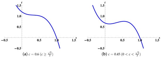
Figure 1. Two possible shapes of $f\left(x\right)$. We fix $a=10,n=3,s_1=0.31,s_2=0.5,d_2=1,k=0.19$.

From the expression of $g\left(x\right)$ in (5), we have $g\left(0\right)=\frac{s_1{d}_2}{d_2-s_2}>0$ when $d_2>s_2$. The asymptotic line of $g\left(x\right)$ is $x=\frac{d_2-s_2}{k}\triangleq x_0$. As $x\to \infty$, $g\left(x\right)\to s_1$. From the expression of $g^{\prime }\left(x\right)$ in (6), we have $g^{\prime }\left(x\right)>0$ and $g^{″}\left(x\right)=\frac{2s_1{s}_2{k}^2}{{(d_2-s_2-kx)}^3}>0$ for $0<x<\tilde{x}$. So $f\left(x\right)$ is a convex function in the interval $(0,\tilde{x})$.

The above analysis can be summarized into the following results:

Case (a): $c\ge \frac{\sqrt{3}}{3}$.

A1. If $f\left(0\right)\ge g\left(0\right)$, then there exists one intersection point of $f\left(x\right)$ and $g\left(x\right)$.

A2. If $f\left(0\right)<g\left(0\right)$, then there is no intersection point of $f\left(x\right)$ and $g\left(x\right)$.

Case (b): $0<c<\frac{\sqrt{3}}{3}$.

In order to find the intersection point of $f\left(x\right)$ and $g\left(x\right)$, we study the critical point in which $f\left(x\right)$ and $g\left(x\right)$ are tangent. We set

$$f^{\prime }\left(x\right)=g^{\prime }\left(x\right),\mathrm{i}.\mathrm{e}.,\frac{a}{n}(-3x^2+2x-c^2)=\frac{s_1{s}_{2}k}{{(d_2-s_2-kx)}^2},$$

(7)

and

$$f\left(x\right)=g\left(x\right),\mathrm{i}.\mathrm{e}.,\frac{a(1-x)(x^2+c^2)}{n}=\frac{s_1(d_2-kx)}{d_2-s_2-kx}.$$

(8)

We suppose that $x^{+}$ is a root of the equation in (7), and we show the existence of $x^{+}$ as follows. Firstly, we study the interaction point of $f^{\prime }\left(x\right)$ and $g^{\prime }\left(x\right)$.

Case (1): If $f^{\prime }\left(\frac{1}{3}\right)<g^{\prime }\left(\frac{1}{3}\right)$, i.e., $\frac{a}{n}(\frac{1}{3}-c^2)<\frac{s_1{s}_{2}k}{{(d_2-s_2-\frac{1}{3}k)}^2}$, then there is no intersection point of $f^{\prime }\left(x\right)$ and $g^{\prime }\left(x\right)$ (see Figure 2a).

Case (2): If $f^{\prime }\left(\frac{1}{3}\right)=g^{\prime }\left(\frac{1}{3}\right)$, i.e., $\frac{a}{n}(\frac{1}{3}-c^2)=\frac{s_1{s}_{2}k}{{(d_2-s_2-\frac{1}{3}k)}^2}$, then there exists one intersection point of $f^{\prime }\left(x\right)$ and $g^{\prime }\left(x\right)$ (see Figure 2b).

Case (3): If $f^{\prime }\left(\frac{1}{3}\right)>g^{\prime }\left(\frac{1}{3}\right)$, i.e., $\frac{a}{n}(\frac{1}{3}-c^2)>\frac{s_1{s}_{2}k}{{(d_2-s_2-\frac{1}{3}k)}^2}$, then there exist two intersection points of $f^{\prime }\left(x\right)$ and $g^{\prime }\left(x\right)$ (see Figure 2c). We suppose that these two intersection points are $x_1^{+}$ and $x_2^{+}$ ($x_{1,2}^{+}$). Then we have $x_1<x_1^{+}<\frac{1}{3}<x_2^{+}<x_2$. When x is a root of both Equations (7) and (8), $f\left(x\right)$ and $g\left(x\right)$ will be tangent.

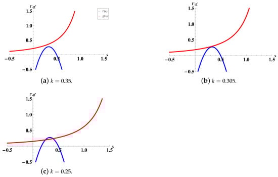
Figure 2. The relative positions of $f^{\prime }\left(x\right)$ and $g^{\prime }\left(x\right)$ depending on k. We fix $a=10,n=3,$ $s_1=0.31,s_2=0.5,d_2=1,c=0.5$.

Next, we discuss the intersection point of $f\left(x\right)$ and $g\left(x\right)$ as follows.

B1. When $f\left(0\right)\ge g\left(0\right)$, i.e., $\frac{a{c}^2}{n}\ge \frac{s_1{d}_2}{d_2-s_2}$, there exists at least one intersection point (since when $x\to \frac{d_2-s_2}{k}$, $g\left(x\right)\to +\infty$).

Case B1.1. When $f^{\prime }\left(\frac{1}{3}\right)<g^{\prime }\left(\frac{1}{3}\right)$, then $f\left(x\right)$ and $g\left(x\right)$ only have one intersection point. In fact, if $f\left(x\right)$ and $g\left(x\right)$ have two intersection points $x_3$ and $x_4$ (that is, $F\left(x_3\right)=F\left(x_4\right)$ where $F\left(x\right)=f\left(x\right)-g\left(x\right)$), then by intermediate value theorem, there exists $\eta \in (x_3,x_4)$, such that $F^{\prime }\left(\eta \right)=0$, i.e., $f^{\prime }\left(\eta \right)=g^{\prime }\left(\eta \right)$. It is a contradiction.

Case B1.2. When $f^{\prime }\left(\frac{1}{3}\right)=g^{\prime }\left(\frac{1}{3}\right)$, there exists at least one intersection point.

Case B1.3. When $f^{\prime }\left(\frac{1}{3}\right)>g^{\prime }\left(\frac{1}{3}\right)$, note that $x_{1,2}^{+}$ satisfies (7), and we have

$f\left(x_{1,2}^{+}\right)=\frac{a(1-x_{1,2}^{+})({\left(x_{1,2}^{+}\right)}^2+c^2)}{n}$ and $g\left(x_{1,2}^{+}\right)=\frac{s_1(d_2-k{x}_{1,2}^{+})}{d_2-s_2-k{x}_{1,2}^{+}}$, then we have the following cases:

(a)

If $f\left(x_1^{+}\right)>g\left(x_1^{+}\right)$, there exists one intersection point (see Figure 3a).

(b)

If $f\left(x_1^{+}\right)=g\left(x_1^{+}\right)$, there exist two intersection points (see Figure 3b).

(c)

If $f\left(x_1^{+}\right)<g\left(x_1^{+}\right)$, $f\left(x_2^{+}\right)>g\left(x_2^{+}\right)$, there exist three intersection points (see Figure 3c).

(d)

If $f\left(x_2^{+}\right)=g\left(x_2^{+}\right)$, there exist two intersection points (see Figure 3d).

(e)

If $f\left(x_2^{+}\right)<g\left(x_2^{+}\right)$, there exists one intersection point (see Figure 3e).

B2. When $f\left(0\right)<g\left(0\right)$, i.e., $\frac{a{c}^2}{n}<\frac{s_1{d}_2}{d_2-s_2}$, we have the following cases:

Case B2.1. When $f^{\prime }\left(\frac{1}{3}\right)\le g^{\prime }\left(\frac{1}{3}\right)$, i.e., $\frac{a}{n}(\frac{1}{3}-c^2)<\frac{s_1{s}_{2}k}{{(d_2-s_2-\frac{1}{3}k)}^2}$, there is no intersection point (see Figure 3f).

Case B2.2. When $f^{\prime }\left(\frac{1}{3}\right)>g^{\prime }\left(\frac{1}{3}\right)$, i.e., $\frac{a}{n}(\frac{1}{3}-c^2)>\frac{s_1{s}_{2}k}{{(d_2-s_2-\frac{1}{3}k)}^2}$ (we know $f\left(x_1\right)<g\left(x_1\right)$, $f\left(x_1^{+}\right)<g\left(x_1^{+}\right)$).

(a)

If $f\left(x_2^{+}\right)<g\left(x_2^{+}\right)$, there is no intersection point (see Figure 3g).

(b)

If $f\left(x_2^{+}\right)=g\left(x_2^{+}\right)$, there exists one intersection point (see Figure 3h).

(c)

If $f\left(x_2^{+}\right)>g\left(x_2^{+}\right)$, there exist two intersection points (see Figure 3i).

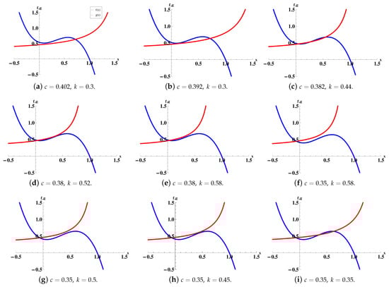
Figure 3. The interactions of $f\left(x\right)$ and $g\left(x\right)$, illustrating the possible number of equilibrium points. We choose $a=10,n=3,s_1=0.23,s_2=0.5,d_2=1$.

2.3. Stability of Equilibria

In order to investigate the local stability of the equilibria of system (3), we linearize the system and obtain the characteristic equation evaluated at a typical equilibrium $\overline{E}=(\overline{x},\overline{y},\overline{z})$.

$$\det \left(\begin{array}{ccc}a-2a\overline{x}-\frac{n\overline{y}(c^2-{\overline{x}}^2)}{{({\overline{x}}^2+c^2)}^2}-\lambda & -\frac{n\overline{x}}{{\overline{x}}^2+c^2}& 0\\ 0& \overline{z}-1-\lambda & \overline{y}\\ k\overline{z}& 0& k\overline{x}-d_2-\lambda \end{array}\right)=0.$$

(9)

At $E_0$, characteristic Equation (9) becomes

$$\left[\lambda -\left(a-\frac{n{y}_0}{c^2}\right)\right]\left[\lambda -\left(\frac{s_2}{d_2}-1\right)\right](\lambda +d_2)=0.$$

Three eigenvalues are ${\lambda }_1=a-\frac{n{y}_0}{c^2}$, ${\lambda }_2=\frac{s_2}{d_2}-1<0$, ${\lambda }_3=-d_2<0$. Note that the feasibility of $E_0$ is $s_2<d_2$. It is easy to show that ${\lambda }_1<0$ if $a<\frac{n{s}_1{d}_2}{(d_2-s_2)c^2},\mathrm{i}.\mathrm{e}.,c<\sqrt{\frac{n{s}_1{d}_2}{a(d_2-s_2)}}$. Therefore, we have the following result.

Theorem 1.

System (3) has one tumor-free equilibrium $E_0$, which is locally asymptotically stable (LAS) if $s_2<d_2$ and $a<\frac{n{s}_1{d}_2}{(d_2-s_2)c^2}$.

Note that $n{y}^{\ast }=a(1-x^{\ast })({x^{\ast }}^2+c^2)$, $y^{\ast }=\frac{s_1}{1-z^{\ast }}$, $\frac{s_2}{z^{\ast }}=d_2-k{x}^{\ast }$ for $E^{\ast }=(x^{\ast },y^{\ast },z^{\ast })$, so the feasibility of equilibrium components requires that $x^{\ast }<1$, $z^{\ast }<1$.

At $E^{\ast }$, characteristic Equation (9) becomes

$${\lambda }^3+b_1{\lambda }^2+b_2\lambda +b_3=0,$$

(10)

where

$$\begin{array}{cc}\hfill b_1& =-\frac{a{x}^{\ast }(-3{x^{\ast }}^2+2x^{\ast }-c^2)}{{x^{\ast }}^2+c^2}+1-z^{\ast }+\frac{s_2}{z^{\ast }},\hfill \\ \hfill b_2& =-\frac{a{x}^{\ast }(-3{x^{\ast }}^2+2x^{\ast }-c^2)}{{x^{\ast }}^2+c^2}(1-z^{\ast }+\frac{s_2}{z^{\ast }})+(1-z^{\ast })\frac{s_2}{z^{\ast }},\hfill \\ \hfill b_3& =-\frac{a{x}^{\ast }(-3{x^{\ast }}^2+2x^{\ast }-c^2)}{{x^{\ast }}^2+c^2}(1-z^{\ast })\frac{s_2}{z^{\ast }}+k{z}^{\ast }\frac{n{x}^{\ast }{y}^{\ast }}{{x^{\ast }}^2+c^2}.\hfill \end{array}$$

(11)

By some algebraic calculations, we find

$$b_1>0\iff 1-z^{\ast }+\frac{s_2}{z^{\ast }}>\frac{a{x}^{\ast }(-3{x^{\ast }}^2+2x^{\ast }-c^2)}{{x^{\ast }}^2+c^2},$$

(12)

$$b_3>0\iff k{z}^{\ast }n{y}^{\ast }>a(-3{x^{\ast }}^2+2x^{\ast }-c^2)(1-z^{\ast })\frac{s_2}{z^{\ast }},$$

(13)

and

$$\begin{array}{cc}\hfill & b_1{b}_2-b_3>0\hfill \\ \hfill & \iff \frac{a^2{x^{\ast }}^2{(-3{x^{\ast }}^2+2x^{\ast }-c^2)}^2}{{({x^{\ast }}^2+c^2)}^2}(1-z^{\ast }+\frac{s_2}{z^{\ast }})\hfill \\ \hfill & -\frac{a{x}^{\ast }(-3{x^{\ast }}^2+2x^{\ast }-c^2)}{{x^{\ast }}^2+c^2}{(1-z^{\ast }+\frac{s_2}{z^{\ast }})}^2\hfill \\ \hfill & +(1-z^{\ast }+\frac{s_2}{z^{\ast }})(1-z^{\ast })\frac{s_2}{z^{\ast }}-k{z}^{\ast }\frac{n{x}^{\ast }{y}^{\ast }}{{x^{\ast }}^2+c^2}>0.\hfill \end{array}$$

(14)

By Routh–Hurwitz criteria, $E^{\ast }$ is stable if the conditions (12)–(14) hold. Therefore, we have the following results.

Theorem 2.

System (3) has at most three tumor-presence equilibria $E^{\ast }$, which are LAS if the conditions (12)–(14) hold.

3. Local Bifurcation Analysis

In this section, we carry out a bifurcation analysis including saddle-node bifurcation, transcritical bifurcation and Hopf bifurcation.

3.1. Saddle-Node Bifurcation

Consider the dimensionless model (3). y- and z-nullclines are given by

$$z=\frac{s_2}{g_1\left(x\right)},y=\frac{s_1{g}_1\left(x\right)}{g_1\left(x\right)-s_2},$$

where $g_1\left(x\right)=d_2-kx$. Then, the nontrivial x-nullcline is given by

$$y=\frac{a}{n}(1-x)f_1\left(x\right),$$

where $f_1\left(x\right)=x^2+c^2$. If $E^{\ast }(x^{\ast },y^{\ast },z^{\ast })$ denotes a typical coexistence equilibrium point, then $x^{\ast }$ is a positive root of the equation

$$\begin{array}{c}\hfill \mathrm{\Phi }\left(x\right)\equiv a(1-x)-\frac{n{s}_1{g}_1\left(x\right)}{f_1\left(x\right)(g_1\left(x\right)-s_2)}=0.\end{array}$$

(15)

Let us assume that the system undergoes a saddle-node bifurcation at $E^{\ast }$, then $x^{\ast }$ should be a double root of the equation $\mathrm{\Phi }\left(x\right)=0$, which requires

$$\begin{array}{c}\hfill \mathrm{\Phi }\left(x^{\ast }\right)=0,{\mathrm{\Phi }}^{\prime }\left(x^{\ast }\right)=0.\end{array}$$

(16)

We can prove that the Jacobian matrix of system (3) evaluated at $E^{\ast }$ should have a simple zero eigenvalue when the conditions in (16) are satisfied. The Jacobian matrix for system (3) evaluated at $E^{\ast }$ is given by

$$\begin{array}{c}\hfill J^{\ast }=\left[\begin{array}{ccc}{x}^{\ast }\left(-a+\frac{n{y}^{\ast }{f}_1^{\prime }\left(x^{\ast }\right)}{f_1^2\left(x^{\ast }\right)}\right)& -\frac{n{x}^{\ast }}{f_1\left(x^{\ast }\right)}& 0\\ 0& z^{\ast }-1& y^{\ast }\\ -z^{\ast }{g}_1^{\prime }\left(x^{\ast }\right)& 0& -g_1\left(x^{\ast }\right)\end{array}\right],\end{array}$$

(17)

where

$$y^{\ast }=\frac{s_1{g}_1\left(x^{\ast }\right)}{g_1\left(x^{\ast }\right)-s_2},z^{\ast }=\frac{s_2}{g_1\left(x^{\ast }\right)}.$$

Now we calculate the determinant of $J^{\ast }$ as follows:

$$\begin{array}{ccc}\hfill det\left(J^{\ast }\right)& =& x^{\ast }\left(-a+\frac{n{y}^{\ast }{f}_1^{\prime }\left(x^{\ast }\right)}{f_1^2\left(x^{\ast }\right)}\right)(1-z^{\ast })g_1\left(x^{\ast }\right)+\frac{n{x}^{\ast }}{f_1\left(x^{\ast }\right)}{y}^{\ast }{z}^{\ast }{g}_1^{\prime }\left(x^{\ast }\right)\hfill \\ & =& x^{\ast }\left(-a+\frac{n{s}_1{g}_1\left(x^{\ast }\right)f_1^{\prime }\left(x^{\ast }\right)}{f_1^2\left(x^{\ast }\right)(g_1\left(x^{\ast }\right)-s_2)}\right)(g_1\left(x^{\ast }\right)-s_2)+\frac{n{x}^{\ast }{s}_1{s}_2{g}_1^{\prime }\left(x^{\ast }\right)}{(g_1\left(x^{\ast }\right)-s_2)}.\hfill \end{array}$$

And we obtain from ${\mathrm{\Phi }}^{\prime }\left(x^{\ast }\right)=0$ that

$$-a+\frac{n{s}_1{g}_1\left(x^{\ast }\right)f_1^{\prime }\left(x^{\ast }\right)}{f_1^2\left(x^{\ast }\right)(g_1\left(x^{\ast }\right)-s_2)}=-\frac{n{s}_1{s}_2{g}_1^{\prime }\left(x^{\ast }\right)}{{(g_1\left(x^{\ast }\right)-s_2)}^2}.$$

Hence, we can find

$$\begin{array}{c}\hfill det\left(J^{\ast }\right)=-x^{\ast }\frac{n{s}_1{s}_2{g}_1^{\prime }\left(x^{\ast }\right)}{{(g_1\left(x^{\ast }\right)-s_2)}^2}(g_1\left(x^{\ast }\right)-s_2)+\frac{n{x}^{\ast }{s}_1{s}_2{g}_1^{\prime }\left(x^{\ast }\right)}{(g_1\left(x^{\ast }\right)-s_2)}=0.\end{array}$$

Next, we have to verify the transversality conditions. The eigenvectors associated with the zero eigenvalue of the matrices $J^{\ast }$ and ${\left(J^{\ast }\right)}^T$ are given by

$$V=\left[\begin{array}{c}1\\ -\frac{s_1{s}_2{g}_1^{\prime }\left(x^{\ast }\right)}{{(g_1\left(x^{\ast }\right)-s_2)}^2}\\ -\frac{s_2{g}_1^{\prime }\left(x^{\ast }\right)}{g_1^2\left(x^{\ast }\right)}\end{array}\right],W=\left[\begin{array}{c}1\\ -\frac{n{x}^{\ast }{g}_1\left(x^{\ast }\right)}{f_1\left(x^{\ast }\right)(g_1\left(x^{\ast }\right)-s_2)}\\ -\frac{n{s}_1{x}^{\ast }{g}_1\left(x^{\ast }\right)}{f_1\left(x^{\ast }\right){(g_1\left(x^{\ast }\right)-s_2)}^2}\end{array}\right].$$

Here, we assume k as the bifurcation parameter. Then $k_{SN}$ is a threshold of k such that the condition (16) is satisfied and $E^{\ast }$ is evaluated at $k_{SN}$. Following the same notations as in [34], we have to check the transversality conditions.

First, we calculate

$$\begin{array}{c}\hfill W^T{F}_k(E^{\ast };k_{SN})=W^T\left[\begin{array}{c}0\\ 0\\ z^{\ast }{x}^{\ast }\end{array}\right]=-\frac{n{s}_1{s}_2{\left(x^{\ast }\right)}^2}{f_1\left(x^{\ast }\right){(g_1\left(x^{\ast }\right)-s_2)}^2}\ne 0,\end{array}$$

(18)

where

$$\begin{array}{c}\hfill F\equiv \left[\begin{array}{c}x\left(a(1-x)-\frac{ny}{x^2+c^2}\right)\\ s_1-y+yz\\ s_2-z(d_2-kx)\end{array}\right],\end{array}$$

(19)

and $F_k$ is the partial derivative of F with respect to k.

After some lengthy algebraic calculation, we can verify that

$$\begin{array}{c}\hfill W^T\left[D^{2}F(E^{\ast };k_{SN})(V,V)\right]\ne 0.\end{array}$$

(20)

Hence, the saddle-node bifurcation is nondegenerate. Therefore, we have the following result.

Theorem 3.

System (3) undergoes a saddle-node bifurcation at $E^{\ast }$ for $k=k_{SN}$, where $k_{SN}$ satisfies the condition (16).

3.2. Transcritical Bifurcation

Consider the dimensionless model (3). The axial equilibrium point is given by $E_0=\left(0,\frac{s_1{d}_2}{d_2-s_2},\frac{s_2}{d_2}\right)$, and the Jacobian matrix of system (3) evaluated at $E_0$ is given by

$$\begin{array}{c}\hfill J_0=\left[\begin{array}{ccc}a-\frac{n{s}_1{d}_2}{(d_2-s_2)c^2}& 0& 0\\ 0& \frac{s_2}{d_2}-1& \frac{s_1{d}_2}{d_2-s_2}\\ \frac{k{s}_2}{d_2}& 0& -d_2\end{array}\right].\end{array}$$

(21)

$E_0$ is feasible for $d_2>s_2$, and hence, two eigenvalues of $J_0$ are ${\lambda }_2=\frac{s_2}{d_2}-1<0$ and ${\lambda }_3=-d_2<0$, and the third eigenvalue is ${\lambda }_1=a-\frac{n{s}_1{d}_2}{(d_2-s_2)c^2}$. Boundary equilibrium point $E_0$ is stable for $a<\frac{n{s}_1{d}_2}{(d_2-s_2)c^2}$ and is unstable if the inequality is reversed. $E_0$ undergoes a transcritical bifurcation at $a_{TC}=\frac{n{s}_1{d}_2}{(d_2-s_2)c^2}$, and $E^{\ast }$ bifurcates from $E_0$ for $a>a_{TC}$. ${\lambda }_1$ is a simple eigenvalue of $J_0$ when $a>a_{TC}$.

The eigenvectors associated with the zero eigenvalue of $J_0$ and $J_0^T$ are given by

$$V=\left[\begin{array}{c}\frac{{(d_2-s_2)}^2}{k{s}_1{s}_2}\\ 1\\ \frac{{(d_2-s_2)}^2}{s_1{d}_2^2}\end{array}\right],W=\left[\begin{array}{c}1\\ 0\\ 0\end{array}\right].$$

Following the same notations as in [34], we have to check the transversality conditions. First, we calculate

$$\begin{array}{c}\hfill W^T{F}_a(E_0;a_{TC})=W^T{\left[\begin{array}{c}x-x^2\\ 0\\ 0\end{array}\right]}_{E_0}=0,\end{array}$$

(22)

where F is defined in (19) and $F_a$ is the partial derivative of F with respect to a.

Next, we can calculate

$$\begin{array}{c}\hfill W^T\left[D{F}_a(E_0;a_{TC})V\right]=\frac{{(d_2-s_2)}^2}{k{s}_1{s}_2}\ne 0,\end{array}$$

(23)

and

$$\begin{array}{c}\hfill W^T\left[D^{2}F(E_0;a_{TC})(V,V)\right]=-\frac{2{(d_2-s_2)}^2}{k{s}_1{s}_2}\left(\frac{a}{k{s}_1{s}_2}+\frac{n}{c^2}\right)\ne 0.\end{array}$$

(24)

Hence, all the transversality conditions are satisfied and the transcritical bifurcation is nondegenerate. Therefore, we have the following result.

Theorem 4.

System (3) exhibits a transcritical bifurcation for $a>a_{TC}$, where $a_{TC}=\frac{n{s}_1{d}_2}{(d_2-s_2)c^2}$.

3.3. Hopf Bifurcation

In order to discuss how system (3) undergoes Hopf bifurcation near the tumor-presence equilibrium $E^{\ast }$, we choose k as a bifurcation parameter and define

$$\varphi \left(k\right)=b_1\left(k\right)b_2\left(k\right)-b_3\left(k\right),$$

where $b_1,b_2$ and $b_3$ are given in (11). Without loss of generality, we suppose that $k=k_H$ such that

$$\varphi \left(k_H\right)=(b_1\left(k\right)b_2\left(k\right)-b_3\left(k\right)){|}_{k=k_H}=0.$$

Under the assumption $b_1{b}_2-b_3=0,b_1>0$ and $b_2>0$, we have that characteristic Equation (9) has one negative eigenvalue $-b_1$ and two purely imaginary eigenvalues $\pm i\omega$, where $\omega >0$ is a real number and satisfies ${\omega }^2=b_2$. By the assumption that $k=k_H$ and $b_2\left(k_H\right)>0$, characteristic Equation (9) becomes

$$({\lambda }^2+b_2)(\lambda +b_1)=0,$$

(25)

which has three roots

$${\lambda }_1=i\sqrt{b_2\left(k_H\right)},{\lambda }_2=-i\sqrt{b_2\left(k_H\right)},{\lambda }_3=-b_1\left(k_H\right).$$

When $0<|k-k_H|\ll 1$, the roots can be expressed as the general form

$${\lambda }_1\left(k\right)=\mu \left(k\right)+i\nu \left(k\right),{\lambda }_2\left(k\right)=\mu \left(k\right)-i\nu \left(k\right),{\lambda }_3\left(k\right)=-b_1\left(k\right)<0,$$

where $\mu \left(k_H\right)=0,\nu \left(k_H\right)=\sqrt{b_2\left(k_H\right)}$.

Next, we verify the transversality condition. Substituting ${\lambda }_1\left(k\right)=\mu \left(k\right)+i\nu \left(k\right)$ into the characteristic Equation (9), calculating the derivative with respect to k at $k_H$ and separating the real and imaginary parts, we achieve that

$$\begin{array}{cc}\hfill (b_2\left(k_H\right)-3{\nu }^2\left(k_H\right)){\mu }^{\prime }\left(k_H\right)-2b_1\left(k_H\right)\nu \left(k_H\right){\nu }^{\prime }\left(k_H\right)+{b_3}^{\prime }\left(k_H\right)-{\nu }^2\left(k_H\right){b_1}^{\prime }\left(k_H\right)& =0\hfill \\ \hfill 2b_1\left(k_H\right)\nu \left(k_H\right){\mu }^{\prime }\left(k_H\right)+(b_2\left(k_H\right)-3{\nu }^2\left(k_H\right)){\nu }^{\prime }\left(k_H\right)+\nu \left(k_H\right){b_2}^{\prime }\left(k_H\right)& =0.\hfill \end{array}$$

(26)

Since $\nu \left(k_H\right)=\sqrt{b_2\left(k_H\right)}$, by eliminating ${\nu }^{\prime }\left(k_H\right)$ in (26), we obtain that

$$\begin{array}{cc}\hfill \frac{\mathrm{d}\mu \left(k\right)}{\mathrm{d}k}{|}_{k=k_H}& =-\frac{(b_2\left(k_H\right)-3{\nu }^2\left(k_H\right))({b_3}^{\prime }\left(k_H\right)-{\nu }^2\left(k_H\right){b_1}^{\prime }\left(k_H\right))+2b_1\left(k_H\right){\nu }^2\left(k_H\right){b_2}^{\prime }\left(k_H\right)}{{(b_2\left(k_H\right)-3{\nu }^2\left(k_H\right))}^2+4{\nu }^2\left(k_H\right)b_1^2\left(k_H\right)}\hfill \\ \hfill & =-\frac{{b_1}^{\prime }\left(k_H\right)b_2\left(k_H\right)+{b_2}^{\prime }\left(k_H\right)b_1\left(k_H\right)-{b_3}^{\prime }\left(k_H\right)}{2(b_1^2\left(k_H\right)+b_2\left(k_H\right))}\hfill \\ \hfill & =-\frac{1}{2(b_1^2\left(k_H\right)+b_2\left(k_H\right))}\frac{\mathrm{d}\varphi \left(k\right)}{\mathrm{d}k}{|}_{k=k_H}.\hfill \end{array}$$

(27)

Therefore, if there exists $k_H>0$ such that $\frac{\mathrm{d}\varphi \left(k\right)}{\mathrm{d}k}{|}_{k=k_H}\ne 0$, then the transversality condition $\frac{\mathrm{d}\mu \left(k\right)}{\mathrm{d}k}{|}_{k=k_H}\ne 0$ can hold. Moreover, since ${\lambda }_3\left(k\right)=-b_1\left(k\right)<0$, Hopf bifurcation can occur at $k=k_H$ by the Hopf bifurcation theorem [35,36]. Therefore, we have the following result.

Theorem 5.

Suppose the tumor-presence equilibrium $E^{\ast }$ exists. If there exists $k_H>0$ such that $b_2\left(k_H\right)>0,\varphi \left(k_H\right)=0$ and $\frac{\mathrm{d}\varphi \left(k\right)}{\mathrm{d}k}{|}_{k=k_H}\ne 0$, system (3) undergoes a Hopf bifurcation near $E^{\ast }$ at $k=k_H$.

4. Numerical Simulations

In this section, we perform numerical simulations to show how parameters k and c affect the dynamics of system (3). Here, the tumor-free equilibrium is named $E_0$. Furthermore, three tumor-presence equilibria are named as follows: low tumor equilibrium $E_1^{\ast }$, intermediate tumor equilibrium $E_2^{\ast }$ and high tumor equilibrium $E_3^{\ast }$. We choose the following parameter set [11,20,22]:

$$a=10,n=3,s_1=0.31,s_2=0.5,d_2=1.$$

(28)

First, we provide the biparametric bifurcation diagram showing the Bogdanov–Takens (BT) bifurcation point where the Hopf bifurcation curve meets with the saddle-node bifurcation curve (see Figure 4). Furthermore, two saddle-node bifurcation curves intersect at the cusp point (CP). On one branch of the Hopf bifurcation, curve we find a generalized Hopf bifurcation point, which is marked as GH.

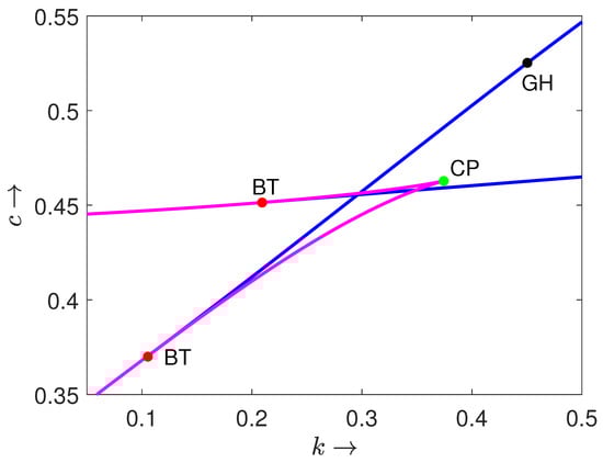
Figure 4. The biparametric bifurcation diagram of system (3) in $(k,c)$ plane. Magenta and blue curves are saddle-node bifurcation and Hopf bifurcation, respectively. BT, CP and GH denote Bogdanov–Takens bifurcation point, cusp bifurcation point and generalized Hopf bifurcation point, respectively.

Next, we provide the bifurcation diagrams of variable x with respect to k by choosing the six different fixed values of $c=0.35,0.43,0.44,0.45,0.46,0.464$. We find that system (3) can undergo saddle-node bifurcation and Hopf bifurcation (see Figure 5).

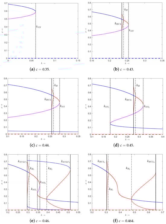
Figure 5. The bifurcation diagrams of x with respect to the parameter k of system (3) with different values of $c=0.35,0.43,0.44,0.45,0.46,0.464$. Solid and dashed curves represent tumor-presence equilibrium and tumor-free equilibrium, respectively. Blue and red (magenta) curves correspond to stable equilibrium and unstable equilibrium, respectively. Saddle-node bifurcation points are labeled as $SN$, $S{N}_1$ and $S{N}_2$. Hopf bifurcation points are labeled as $H_1$ and $H_2$. Homoclinic bifurcation thresholds are labeled as $HCL$, $HC{L}_1$ and $HC{L}_2$. Saddle-node bifurcation of periodic orbits are denoted as $SNL{C}_1$ and $SNL{C}_2$.

Case 1: $c=0.35$ (satisfying $f\left(0\right)<g\left(0\right)$, see Figure 5a).

• There is one saddle-node bifurcation point named $k_{SN}=0.0589$. For any $k>0$, the tumor-free equilibrium $E_0$ always exists, which is stable. When $0<k<k_{SN}$, there exist two tumor-presence equilibria: unstable $E_2^{\ast }$ and stable $E_3^{\ast }$. Furthermore, we find the bistability of $E_0$ and $E_3^{\ast }$.

Case 2: $c=0.43$ (satisfying $f\left(0\right)<g\left(0\right)$, see Figure 5b).

• There is one saddle-node bifurcation point named $k_{SN}=0.2538$ and one Hopf bifurcation point named $k_H=0.2398$. For any $k>0$, $E_0$ always exists, which is stable. When $0<k<k_{SN}$, there exist $E_2^{\ast }$ and $E_3^{\ast }$, where $E_2^{\ast }$ is unstable. $E_3^{\ast }$ is stable when $0<k<k_H$ and unstable when $k_H<k<k_{SN}$. Furthermore, we find that the Hopf bifurcating limit cycle disappears through a homoclinic bifurcation $k_{HCL}$.

Case 3: $c=0.44$ (satisfying $f\left(0\right)>g\left(0\right)$, see Figure 5c).

• There is one saddle-node bifurcation point named $k_{SN}=0.2835$ and a Hopf bifurcation point named $k_H=0.261$. For any $k>0$, $E_0$ always exists, which is unstable. When $0<k<k_{SN}$, there exist $E_1^{\ast }$, $E_2^{\ast }$ and $E_3^{\ast }$, where $E_1^{\ast }$ is stable and $E_2^{\ast }$ is unstable. $E_3^{\ast }$ is stable when $0<k<k_H$ and unstable when $k_H<k<k_{SN}$. When $k>k_{SN}$, there exists $E_1^{\ast }$, which is stable.

Case 4: $c=0.45$ (satisfying $f\left(0\right)>g\left(0\right)$, see Figure 5d).

• There are two saddle-node bifurcation points named $k_{SN1}=0.1774$ and $k_{SN2}=0.3171$ and one Hopf bifurcation point named $k_H=0.284$. For any $k>0$, $E_0$ always exists, which is unstable. When $0<k<k_{SN1}$, there exists $E_3^{\ast }$, which is stable. When $k_{SN1}<k<k_{SN2}$, there exist $E_1^{\ast }$, $E_2^{\ast }$ and $E_3^{\ast }$, where $E_1^{\ast }$ is stable and $E_2^{\ast }$ is unstable. $E_3^{\ast }$ is stable when $k_{SN1}<k<k_H$ and unstable when $k_H<k<k_{SN2}$. When $k>k_{SN2}$, there exists $E_1^{\ast }$, which is stable. By fixing $k=0.19(k_{SN1}<0.19<k_H)$, we can obtain $E_1^{\ast }(0.1314,0.6363,0.5128)$, $E_2^{\ast }(0.189,0.644,0.5186)$, $E_3^{\ast }(0.6593,0.7236,0.5716)$ and find the bistability of $E_1^{\ast }$ and $E_3^{\ast }$.

Case 5: $c=0.46$ (satisfying $f\left(0\right)>g\left(0\right)$, see Figure 5e).

• There are saddle-node bifurcation points named $k_{SN1}=0.347$ and $k_{SN2}=0.3586$ and two Hopf bifurcation points named $k_{H1}=0.306$ and $k_{H2}=0.3927$. For any $k>0$, $E_0$ always exists, which is unstable. When $0<k<k_{SN1}$, there exists $E_3^{\ast }$. $E_3^{\ast }$ is stable when $0<k<k_{H1}$, and unstable when $k_{H1}<k<k_{SN1}$. When $k_{SN1}<k<k_{SN2}$, there exist $E_1^{\ast }$, $E_2^{\ast }$ and $E_3^{\ast }$, where they are all unstable. When $k>k_{SN2}$, there exists $E_1^{\ast }$. $E_1^{\ast }$ is unstable when $k_{SN2}<k<k_{H2}$ and stable when $k>k_{H2}$. By fixing $k=0.39(k_{H1}<0.39<k_{H2})$, we can obtain $E_1^{\ast }=(0.1598,0.6641,0.5332)$ and find stable periodic solutions around $E_1^{\ast }$ (see Figure 6). Furthermore, we find two homoclinic bifurcation thresholds $k_{HCL1}$ and $k_{HCL2}$ in this case.

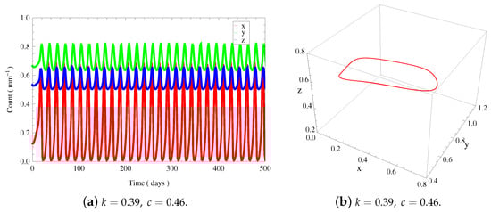
Figure 6. (a) The time evolution curves of $x,y,z$ of system (3) around $E_1^{\ast }=(0.1598,0.6641,0.5332)$, which show periodic oscillations. (b) The 3D phase portrait depicts a stable limit cycle corresponding to (a).

Case 6: $c=0.464$ (satisfying $f\left(0\right)>g\left(0\right)$, see Figure 5f).

• There are two Hopf bifurcation points named $k_{H_1}$ and $k_{H_2}$. For any $k>0$, $E_3^{\ast }$ always exists. $E_3^{\ast }$ is stable when $0<k<k_{H1}$ or $k>k_{H2}$ and unstable when $k_{H1}<k<k_{H2}$.

Next, we provide the bifurcation diagrams of variable x with respect to c by choosing the four different typical cases of $k=0.1,0.19,0.3,0.4$. We find that system (3) can appear with saddle-node bifurcation, transcritical bifurcation and Hopf bifurcation (see Figure 7). As k increases, upper saddle-node bifurcation point $c_{SN1}$ will disappear, which means that $E_2^{\ast }$ and $E_3^{\ast }$ will merge, and lower saddle-node bifurcation point $c_{SN2}$ will disappear, which means that $E_1^{\ast }$ and $E_2^{\ast }$ will merge. Furthermore, upper Hopf bifurcation point $c_{H2}$ and lower Hopf bifurcation point $c_{H1}$ will appear one after another, causing the stability switch of $E_3^{\ast }$. As k increases, the curve of $x^{\ast }$ of the tumor-presence equilibrium goes up on the right side, and the upper branch goes down. In the case of $k=0.19$ from Figure 7b, we find two bistable scenarios: $E_0$ and $E_3^{\ast }$ ($c^H<c<c^{TC}$, see Figure 8a,b), and $E_1^{\ast }$ and $E_3^{\ast }$ ($c_{TC}<c<c_{SN2}$, see Figure 8c,d), where $c_H=0.4076,c_{TC}=0.4316,c_{SN2}=0.4506$. For larger values of k (e.g., $k=0.4$), there is only one tumor-presence equilibrium $E^{\ast }$ as c varies (see Figure 7d). Furthermore, we find two Hopf bifurcation points at $c_{H1}=0.464$ and $c_{H2}=0.5381$.

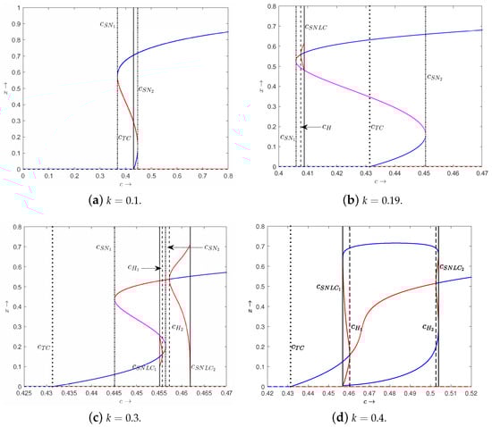
Figure 7. The bifurcation diagrams of x with respect to the parameter c of system (3) with different values of $k=0.1,0.19,0.3,0.4$. Solid and dashed curves represent tumor-presence equilibrium and tumor-free equilibrium, respectively. Blue and red(magenta) curves correspond to stable equilibrium and unstable equilibrium, respectively. Saddle-node bifurcation points are labeled as $SN1$ and $SN2$. Hopf bifurcation points are labeled as H, $H1$ and $H2$. Transcritical bifurcation is labeled as $TC$. Saddle-node bifurcations of periodic orbits are denoted as $SNL{C}_1$ and $SNL{C}_2$.

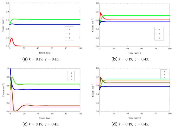
Figure 8. The time evolution curves of $x,y,z$ of system (3). (a,b) show the bistability of $E_0(0,0.62,0.5)$ and $E_3^{\ast }=(0.63,0.7176,0.568)$. (c,d) show the bistability of $E_1^{\ast }(0.1314,0.6363,0.5128)$ and $E_3^{\ast }(0.6593,0.7236,0.5716)$.

When $k=0.19$, we identify five distinct regions separated by four critical points as c varies: two saddle-node bifurcation points $c_{SN1}=0.4059$ and $c_{SN2}=0.4506$, one Hopf bifurcation point $c_H=0.4076$ and one transcritical bifurcation point $c_{TC}=0.4316$ (see Figure 7b). $E_0$ always exists. Furthermore, $E_0$ is stable when $0<c<c_{TC}$ and unstable when $c>c_{TC}$. The qualitative behavior in each region as c varies is summarized as follows:

(1)

$0<c<c_{SN1}$: there is no tumor-presence equilibrium.

(2)

$c=c_{SN1}$: one saddle-node bifurcation point at which $E_2^{\ast }$ and $E_3^{\ast }$ will appear. In this case, the functions $f\left(x\right)$ and $g\left(x\right)$ are tangent.

(3)

$c_{SN1}<c<c_H$: there exist $E_2^{\ast }$ and $E_3^{\ast }$. Both $E_2^{\ast }$ and $E_3^{\ast }$ are unstable.

(4)

$c_H<c<c_{TC}$: there exist $E_2^{\ast }$ and $E_3^{\ast }$. $E_2^{\ast }$ is unstable and $E_3^{\ast }$ is stable.

(5)

$c=c_{TC}$: one transcritical bifurcation point at which $E_0$ loses the stability.

(6)

$c_{TC}<c<c_{SN2}$: there exist $E_1^{\ast }$, $E_2^{\ast }$ and $E_3^{\ast }$. Both $E_1^{\ast }$ and $E_3^{\ast }$ are stable, while $E_2^{\ast }$ is unstable.

(7)

$c=c_{SN2}$: one saddle-node bifurcation at which $E_1^{\ast }$ and $E_2^{\ast }$ will merge. In this case, the functions $f\left(x\right)$ and $g\left(x\right)$ are tangent.

(8)

$c>c_{SN2}$: there exists $E_3^{\ast }$, which is stable.

5. Conclusions and Discussion

In this paper, we proposed a tumor–immune system interaction model with nonmonotonic immune response function in the presence of a large number of tumors. We studied the existence and stability of tumor-free equilibrium $E_0$ and tumor-presence equilibrium $E^{\ast }$ of system (3). Our results showed that $E_0$ undergoes a transcritical bifurcation at $a_{TC}=\frac{n{s}_1{d}_2}{(d_2-s_2)c^2}$ and $E^{\ast }$ bifurcates from $E_0$ for $a>a_{TC}$. We found that system (3) displays a saddle-node bifurcation in which the sudden appearance of an equilibrium point which splits into two equilibria can be found. We also present a biparametric bifurcation diagram to show the appearance of the BT bifurcation point and cusp bifurcation point (see Figure 4). In addition, Hopf bifurcations at $E^{\ast }$ were detected by choosing k (see Figure 5) and c (see Figure 7) as the bifurcation parameter, respectively. The Hopf bifurcation is supercritical and can induce stable periodic solutions (see Figure 6). Interestingly, we also found the bistability of two tumor-presence equilibria named the low-tumor-presence equilibrium and the high-tumor-presence equilibrium (see Figure 8). Two types of bistability phenomena show symmetric and antisymmetric properties in a range of model parameters and initial cell concentrations, which reveals that patients with ACI can possibly reach either a stable tumor-free state or a low-tumor-presence state when the nonmonotonic immune response is properly activated.

The two-dimensional dynamic model proposed by Kuznetsov et al. [20] can also have at most three tumor-presence equilibria with the bistability of small and large tumor-presence equilibria, but the model has no closed orbits, shown by the Dulac–Bendixson criterion [37]. The three-dimensional dynamic model proposed by Dong et al. [11] can also exhibit a Hopf bifurcation inducing stable periodic orbits, but the model has only a unique tumor-presence equilibrium. However, the consideration of nonmonotonic immune response function in our model (3) can capture both the bistability phenomenon and periodic orbits, showing rich dynamics. Comparing the monotonic immune response function to, for example, the saturated type used in the modeling of the immune system against the tumor [21], the nonmonotonic immune response function adopted by this study made the theoretical analysis more challenging while also bringing new, interesting findings. In this study, we only considered the constant input of ACI treatment as one immunotherapy. In further studies, we can introduce other tumor therapies (radiotherapy, chemotherapy, CAR T cell therapy and oncolytic virotherapy) into the model (1) to evaluate the effects of combination treatments for tumor management [38]. In addition, due to proliferation, differentiation and transport of immune cells, the immune system needs some time to be activated, which also plays an important role in tumor–immune system interactions [39].

References

- Vesely, M.D.; Schreiber, R.D. Cancer Immunoediting: Antigens, mechanisms and implications to cancer immunotherapy. Ann. N. Y. Acad. Sci. 2013, 1284, 1–5. [Google Scholar] [CrossRef] [PubMed]
- Yang, Y.L.; Yang, F.; Huang, Z.Q.; Li, Y.Y.; Shi, H.Y.; Sun, Q.; Xu, F.H. T cells, NK cells, and tumor-associated macrophages in cancer immunotherapy and the current state of the art of drug delivery systems. Front. Immunol. 2023, 14, 1199173. [Google Scholar] [CrossRef] [PubMed]
- Beatty, G.L.; Gladney, W.L. Immune escape mechanisms as a guide for cancer immunotherapy. Clin. Cancer Res. 2015, 21, 687–692. [Google Scholar] [CrossRef] [PubMed]
- Kim, S.K.; Cho, S.W. The evasion mechanisms of cancer immunity and drug intervention in the tumor microenvironment. Front. Pharmacol. 2022, 13, 868695. [Google Scholar] [CrossRef] [PubMed]
- Tan, S.; Li, D.; Zhu, Z. T cells, Cancer immunotherapy: Pros, cons and beyond. Biomed. Pharmacother. 2020, 124, 109821. [Google Scholar] [CrossRef] [PubMed]
- Farkona, S.; Diamandis, E.P.; Blasutig, I.M. Cancer immunotherapy: The beginning of the end of cancer? BMC Med. 2016, 14, 73. [Google Scholar] [CrossRef] [PubMed]
- Waldman, A.D.; Fritz, J.M.; Lenardo, M.J. A guide to cancer immunotherapy: From T cell basic science to clinical practice. Nat. Rev. Immunol. 2020, 20, 651–668. [Google Scholar] [CrossRef] [PubMed]
- Eftimie, R.; Bramson, J.L.; Earn, D.J.D. Interactions between the immune system and cancer: A brief review of non-spatial mathematical models. Bull. Math. Biol. 2011, 73, 2–32. [Google Scholar] [CrossRef]
- de Pillis, L.G.; Radunskaya, A.E. A mathematical tumor model with immune resistance and drug therapy: An optimal control approach. Computat. Math. Methods Med. 2001, 3, 79–100. [Google Scholar]
- de Pillis, L.G.; Radunskaya, A.E.; Wiseman, C.L. A validated mathematical model of cell-mediated immune response to tumor growth. Cancer Res. 2005, 65, 7950–7958. [Google Scholar] [CrossRef]
- Dong, Y.; Miyazaki, R.; Takeuchi, Y. Mathematical modeling on helper T cells in a tumor immune system. Discret. Contin. Dyn. Syst. Ser. B 2014, 19, 55–72. [Google Scholar] [CrossRef]
- Wilson, S.; Levy, D. A mathematical model of the enhancement of tumor vaccine efficacy by immunotherapy. Bull. Math. Biol. 2012, 74, 1485–1500. [Google Scholar] [CrossRef]
- den Breems, N.Y.; Eftimie, R. The re-polarisation of M2 and M1 macrophages and its role on cancer outcomes. J. Theor. Biol. 2016, 390, 23–39. [Google Scholar] [CrossRef] [PubMed]
- Shu, Y.; Huang, J.; Dong, Y.; Takeuchi, Y. Mathematical modeling and bifurcation analysis of pro- and anti-tumor macrophages. Appl. Math. Model. 2020, 88, 758–773. [Google Scholar] [CrossRef]
- d’Onofrio, A. Metamodeling tumor-immune systeminteraction, tumor evasion and immunotherapy. Math. Comput. Model. 2008, 47, 614–637. [Google Scholar] [CrossRef]
- Mahlbacher, G.E.; Reihmer, K.C.; Frieboes, H.B. Mathematical modeling of tumor-immune cell interactions. J. Theor. Biol. 2019, 469, 47–60. [Google Scholar] [CrossRef] [PubMed]
- Tao, Y.; Campbell, S.A.; Poulin, F.J. Dynamics of a diffusive nutrient-phytoplankton-zooplankton model with spatio-temporal delay. SIAM J. Appl. Math. 2021, 81, 2405–2432. [Google Scholar] [CrossRef]
- Xu, Q.; Huang, J.; Dong, Y.; Takeuchi, Y. A delayed HIV infection model with the homeostatic proliferation of CD4 +T cells. Acta Math. Appl. Sin. Engl. Ser. 2022, 38, 441–462. [Google Scholar] [CrossRef]
- Tao, Y.; Sun, Y.; Zhu, H.; Lyu, J.; Ren, J. Nilpotent singularities and periodic perturbation of a GIβ model: A pathway to glucose disorder. J. Nonlinear Sci. 2023, 33, 33–49. [Google Scholar] [CrossRef]
- Kuznetsov, V.A.; Makalkin, I.A.; Taylor, M.A.; Perelson, A.S. Nonlinear dynamics of immunogenic tumors: Parameter estimation and global bifurcation analysis. Bull. Math. Biol. 1994, 56, 295–321. [Google Scholar] [CrossRef]
- Kirschner, D.; Panetta, J. Modeling immunotherapy of the tumor-immune interaction. J. Math. Biol. 1998, 37, 235–252. [Google Scholar] [CrossRef] [PubMed]
- Dritschel, H.; Waters, S.L.; Roller, A.; Byrne, H.M. A mathematical model of cytotoxic and helper T cell interactions in a tumour microenvironment. Lett. Biomath. 2018, 5, S36–S68. [Google Scholar] [CrossRef]
- Talkington, A.; Dantoin, C.; Durrett, R. Ordinary differential equation models for adoptive immunotherapy. Bull. Math. Biol. 2018, 80, 1059–1083. [Google Scholar] [CrossRef] [PubMed]
- Song, G.; Liang, G.; Tian, T.; Zhang, X. Mathematical modeling and analysis of tumor chemotherapy. Symmetry 2022, 14, 704. [Google Scholar] [CrossRef]
- Bekker, R.A.; Kim, S.; Pilon-Thomas, S.; Enderling, H. Mathematical modeling of radiotherapy and its impact on tumor interactions with the immune system. Neoplasia 2022, 28, 100796. [Google Scholar] [CrossRef] [PubMed]
- Butner, J.D.; Dogra, P.; Chung, C. Mathematical modeling of cancer immunotherapy for personalized clinical translation. Nat. Comput. Sci. 2022, 2, 785–796. [Google Scholar] [CrossRef] [PubMed]
- Tang, S.; Li, S.; Wang, X.; Xiao, Y.; Checke, R.A. Hormetic and synergistic effects of cancer treatments revealed by modelling combinations of radio-or chemotherapy with immunotherapy. BMC Cancer 2023, 23, 1040. [Google Scholar] [CrossRef] [PubMed]
- Zhang, Y.; Xie, L.; Dong, Y.; Ruan, S.; Takeuchi, Y. Bifurcation analysis in a tumor-immune system interaction model with dendritic cell therapy and immune response delay. SIAM J. Appl. Math. 2023, 83, 1892–1914. [Google Scholar] [CrossRef]
- Elmusrati, A.; Wang, J.; Wang, C.Y. Tumor microenvironment and immune evasion in head and neck squamous cell carcinoma. Int. J. Oral Sci. 2021, 13, 24. [Google Scholar] [CrossRef]
- Vinay, D.S.; Ryan, E.P.; Pawelec, G.; Talib, W.H.; Stagg, J.; Elkord, E.; Kwon, B.S. Immune evasion in cancer: Mechanistic basis and therapeutic strategies. Semin. Cancer Biol. 2015, 35, S185–S198. [Google Scholar] [CrossRef]
- Gonzalez, H.; Hagerling, C.; Werb, Z. Roles of the immune system in cancer: From tumor initiation to metastatic progression. Genes. Dev. 2018, 32, 1267–1284. [Google Scholar] [CrossRef] [PubMed]
- Serre, R.; Benzekry, S.; Padovani, L.; Meille, C.; André, N.; Ciccolini, J.; Barbolosi, D. Mathematical modeling of cancer immunotherapy and its synergy with radiotherapy. Cancer Res. 2016, 76, 4931–4940. [Google Scholar] [CrossRef] [PubMed]
- Yu, M.; Dong, Y.; Takeuchi, Y. Dual role of delay effects in a tumour-immune system. J. Biol. Dyn. 2017, 11, 334–347. [Google Scholar] [CrossRef] [PubMed]
- Perko, L. Differential Equations and Dynamical Systems, 3rd ed.; Springer: New York, NY, USA, 2013. [Google Scholar]
- Ruan, S.; Wolkowicz, G.S.K. Bifurcation analysis of a chemostat model with a distributed delay. J. Math. Anal. Appl. 1996, 204, 786–812. [Google Scholar] [CrossRef]
- Marsden, J.E.; McKracken, M. The Hopf Bifurcation and Its Applications, 1st ed.; Springer: New York, NY, USA, 1976. [Google Scholar]
- Wiggins, S. Introduction to Applied Nonlinear Dynamical Systems and Chaos, 2nd ed.; Springer: New York, NY, USA, 2003. [Google Scholar]
- Malinzi, J.; Basita, K.B.; Padidar, S.; Adeola, H.A. Prospect for application of mathematical models in combination cancer treatments. Int. J. Med. Inform. 2021, 23, 100534. [Google Scholar] [CrossRef]
- Ruan, S. Nonlinear dynamics in tumor-immune system interaction models with delays. Discrete Contin. Dyn. Syst. Ser. B 2021, 26, 541–602. [Google Scholar] [CrossRef]
Disclaimer/Publisher’s Note: The statements, opinions and data contained in all publications are solely those of the individual author(s) and contributor(s) and not of MDPI and/or the editor(s). MDPI and/or the editor(s) disclaim responsibility for any injury to people or property resulting from any ideas, methods, instructions or products referred to in the content. |
© 2024 by the authors. Licensee MDPI, Basel, Switzerland. This article is an open access article distributed under the terms and conditions of the Creative Commons Attribution (CC BY) license (https://creativecommons.org/licenses/by/4.0/).