Abstract
The number of failures serves as a critical indicator that dynamically impacts the reliability of self-announcing failure products, making it highly practical to incorporate the failure count into reliability management throughout the entire product life cycle. This paper investigates comprehensive methodologies for effectively managing the reliability of self-announcing failure products throughout both the warranty and post-warranty stages, taking into account factors such as the failure count, mission cycles, and limited time duration. Three renewable warranty strategies are introduced alongside proposed models for post-warranty replacements. By analyzing variables like the failure number, mission cycles, and time constraints, these proposed warranties provide practical frameworks for efficient reliability management during the warranty stage. Additionally, the introduced warranties utilize cost and time metrics to extract valuable insights that inform decision making and enable effective reliability management during the warranty stage. Moreover, this study establishes cost and time metrics for key post-warranty replacements, facilitating the development of individual cost rates and model applications in other post-warranty scenarios. Analyses of the renewable free-repair–replacement warranties demonstrate that establishing an appropriate number of failures as the replacement threshold can effectively reduce warranty-servicing costs and extend the coverage duration.
1. Introduction
Warranty strategies and post-warranty maintenance models are two types of indispensable tools to manage the life-cycle reliability of products. Manufacturers design warranty strategies and utilize them to effectively manage the warranty-stage reliability. Consumers develop post-warranty maintenance models and employ them to effectively manage reliability beyond the warranty period. Due to their crucial roles in managing product life-cycle reliability through symmetrical actions, both warranty strategies and post-warranty maintenance models have been extensively researched from various perspectives.
Through an extensive analysis of the existing literature, researchers have designed warranty strategies and formulated post-warranty maintenance models to efficiently manage the life-cycle reliability of two distinct product categories. The first type of product is known as a self-announcing failure product, where failure is self-declared by the loss of one or more functionalities. For instance, when a voltage is applied, and the electromotor fails to start, it indicates a loss of functionality, categorizing the electromotor as a self-announcing failure product. The second type of product is referred to as a degradation-based failure product, where failure is initiated when the degradation level falls below or exceeds a failure threshold. For instance, as the wireless network coverage degrades due to usage, the corresponding router will fail when the coverage falls below a specified threshold (failure threshold). This categorizes the router as a degradation-based failure product.
The failure processes of self-announcing failure products are often represented using one or more lifetime-based distribution functions, depending on the specific failure mechanism. For example, Zhang and Xie [1] employed a Weibull distribution to model lifetime data as random variables and examined parameter estimation methods for the upper truncated Weibull distribution. Similarly, Ducros and Pamphile [2] utilized a Weibull mixture model to represent the lifetime data of a two-component mixture and proposed a Bayesian bootstrap method for parameter estimation. The failure processes of degradation-based failure products are characterized as one or more stochastic degradation processes. For example, Song and Cui [3], Wang et al. [4], Ye and Xie [5], Qiu and Cui [6], and Van et al. [7] modeled the failure processes of degradation-based failure products as a Gamma process; Zhang et al. [8], Zhou et al. [9], Ye et al. [10], Mukhopadhyay et al. [11], and Lu et al. [12] modeled the failure processes of degradation-based failure products as a Markov/Wiener process; and Guo et al. [13] and Wang et al. [14] modeled the failure processes of degradation-based failure products as an Inverse Gaussian process.
Three warranty strategies, which are based on maintenance cases, have been designed to manage the warranty-stage reliability of self-announcing failure products. One warranty strategy is the free repair (i.e., minimal repair) warranty (FRW). In this strategy, minimal repairs are performed without affecting the product’s failure rate, and all costs associated with failure removal are borne by the manufacturers (see Chen et al. [15]; Ye et al. [16]; and Qiao et al. [17]). Another warranty strategy is the preventive maintenance warranty (PMW), wherein preventive maintenance (PM) is performed in the form of periodic or nonperiodic time/usage intervals to improve warranty-stage reliability and enhance availability (see Wang et al. [18] and Su et al. [19]). Under this strategy, when a product experiences its first failure, it is replaced with a new, identical product that is sold under the same warranty strategy or a different one with a nonrenewable warranty region (see Liu et al. [20]; Wang et al. [21]; Rao [22]; and Wang et al. [23]). For degradation-based failure products, both RWs have been designed to manage their reliability. For example, using a stochastic degradation process to model the failure processes of degradation-failure products, Shang et al. [24] proposed a RW for managing the warranty-stage reliability of degradation-failure products; likewise, Zhang et al. [25] introduced and modeled a condition-based nonrenewable RW.
Numerous post-warranty maintenance models have been developed based on maintenance cases to manage the reliability of self-announcing failure products after the warranty period, which can be categorized into the following categories: One prominent type of model is the replacement model, wherein age replacements, periodic replacements, and block replacements have been used to manage the post-warranty reliability of self-announcing failure products (see Liu et al. [26] and Park and Pham [27]). Another type of model is the preventive maintenance (PM) model, which utilizes either periodic or non-periodic maintenance to manage the post-warranty reliability of self-announcing failure products (see Park et al. [28]). The combination model, as a third type, integrates both the PM and replacement models to manage the post-warranty reliability of self-announcing failure products (see Shang et al. [29]). Post-warranty maintenance models for degradation-based failure products are also predominantly in the form of combination models, combining condition-based replacement and PM strategies to manage their reliability after the warranty period. For example, Shang et al. [24] proposed a combination model, integrating condition-based replacement and PM for managing the post-warranty reliability of degradation-failure products.
From the perspectives of strategy/model applications, both warranty strategies and post-warranty maintenance models for managing the life-cycle reliability of degradation-failure products rely on a range of digital technologies, such as big data, cloud computing, artificial intelligence, the Internet of Things (IoT), blockchain, and 5G technologies. This is because digital technologies enable the monitoring and logical processing of degradation data. Furthermore, digital technologies enable the precise monitoring and recording of mission cycles and failure information for self-announcing failure products. For instance, digital technologies enable the monitoring and transfer of mission cycles and failure information of new-type charging piles to equipment ledgers through a management system. Similarly, the integration of digital technologies into the management system of new-type e-bikes allows for the monitoring and recording of the mission cycles and failure information specific to these e-bikes.
The failure number of self-announcing failure products is a crucial measure for assessing changes in reliability. Specifically, the number of failures significantly impacts both the maintenance cost and the duration of servicing during the warranty and post-warranty stages. Although Liu and Wang [30] have used the failure number as the warranty term, there are three core focuses that have not been explored: ① the failure number has not been used as the replacement threshold for the renewable free-replacement warranty (RFRW), which belongs to the RW type mentioned above; ② both the failure number and mission cycles have not been incorporated into the terms of post-warranty maintenance models; and ③ the impact of using the failure number as the replacement threshold for RFRWs in managing the warranty-stage reliability of self-announcing failure products, considering mission cycles, has not been investigated.
This study focuses on self-announcing failure products and presents three renewable warranties from the manufacturers’ points of view to effectively manage the reliability of these products during the warranty stage. The first renewable warranty involves a limited failure number that serves as the replacement threshold within the warranty period, which is named a renewable free-repair–replacement warranty (RFRRW). The second renewable warranty, referred to as a two-dimensional, renewable free-repair–replacement warranty first (2DRFRRWF), incorporates two restrictions: the warranty period and limited mission cycles. It still utilizes the limited failure number as the replacement threshold within the warranty coverage, and the warranty coverage is limited by the condition ‘whichever occurs first’. The third renewable warranty, named the two-dimensional, renewable free-repair–replacement warranty last (2DRFRRWL), is introduced by modifying the condition ‘whichever occurs first’ to ‘whichever occurs last’. These three warranties are formulated considering both cost and time measures, aiming to provide valuable insights for effectively managing the warranty stage reliability of self-announcing failure products subject to mission cycles.
In the context of using the boundaries of the 2DRFRRWF region as symmetrical points to divide the life cycle into warranty and post-warranty stages, two post-warranty replacement models are proposed and developed from a consumer perspective to effectively manage the reliability during the post-warranty stage, called post-warranty reliability. The first post-warranty replacement model is proposed and modeled by incorporating the failure number, mission cycle number, and planned time into the post-warranty stage. Because these three parameters are considered as decision variables and ‘whichever occurs first’ can restrict the replacement coverage, this replacement model is referred to as trivariate random replacement first (TRRF). By setting the values of decision variables, two variations of TRRF, i.e., bivariate random replacement first (BRRF) and bivariate random discrete replacement first (BRDRF), are presented. The second post-warranty replacement model is obtained by changing ‘whichever occurs first’ to ‘whichever occurs last’, which is named a trivariate random replacement last (TRRL). Similarly, two variations of TRRL, i.e., bivariate random replacement last (BRRL) and bivariate random discrete replacement last (BRDRL), are presented by setting values of decision variables. Utilizing all the presented warranty strategies and selected proposed post-warranty replacement models as representatives, a numerical analysis is conducted to extract valuable insights.
The novel aspects of this paper are summarized as follows: (a) the RFRRW is modeled to explore the impact of a limited failure number on the warranty coverage and to identify its benefits; (b) the 2DRFRRWF and 2DRFRRWL, are designed and modeled, while also uncovering their advantages in using a limited failure number as the replacement threshold during warranty coverage; (c) the TRRF, TRRL, BRDRF, and BRDRL are defined and modeled to effectively manage the post-warranty reliability of self-announcing failure products subject to mission cycles, which is a topic that has received little attention in the existing literature; and (d) the solutions proposed in this paper not only facilitate the advancement of warranty theory but also represent a novel exploration of warranty models amidst the backdrop of digital transformation.
The paper’s structure is organized as follows: Section 2 shows the designs and models of three renewable warranties by incorporating some of the limited failure number, limited mission cycles, and warranty period or all into the classic RFRW. In Section 3, two trivariate replacement models are designed and modeled to manage the post-warranty reliability, and some of their variants are presented by setting parameter values. Section 4 shows the analyzed numerically representative models. Section 5 concludes the paper.
2. The Design and Modeling of Renewable Warranties
The paper relies on the following commonly used assumptions: the self-announcing failure product, such as an automatically guided vehicle and logistics robot, carries goods at cycles, called mission cycles, throughout the whole paper. The mission cycles () are random variables following a memoryless identical distribution function , where is a realization of . Let be the distribution function of the arrival time of the first failure, where with () and () is the failure rate function. In particular, the products mentioned hereinafter are referred to as self-announcing failure products, and vice versa, and the repair and replacement are instantaneous.
2.1. Design and Modeling of Warranty A
Denoted by a limited non-negative integer and denoted by a non-negative constant, the first warranty includes the following terms:
- If the failure occurs before the warranty period , then the failed product is replaced as a new identical product sold under the present warranty, which is terminated when the failure does not occur until the warranty period ;
- Minimal repairs are used to remove all failures before replacement, and manufacturers completely absorb the costs of the repair and replacement.
Obviously, this warranty can be divided into the following core aspects: the warranty is renewable; the repair and replacement are free to consumers; limited repairs, i.e., repairs, are considered; and the failure is set as the replacement threshold. In view of these, this warranty is called a renewable free-repair–replacement warranty (RFRRW). Such a RFRRW is explicitly displayed in Figure 1.
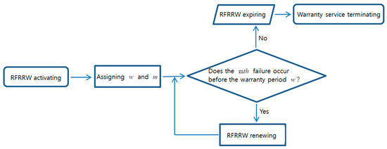
Figure 1.
The graphical representation of the RFRRW.
Let be the arrival time of the failure, which can be computed by summing interval times between failures; then, the distribution and reliability functions of can be modeled as and , respectively, where is the probability that failures occur exactly in the interval and satisfies . The replacement is triggered when the failed product has undergone failures, which have been removed by means of minimal repairs. Let and be the unit repair cost and unit replacement cost, respectively. Because these two costs are borne by the manufacturer, the total cost caused by the unit replacement is given by . In addition, for the product that goes through the RFRRW during the warranty period , the mean value of the failure number is calculated as . Obviously, the replacement process caused by the RFRRW conforms to the characteristics of the geometric distribution. By using the method to calculate the expectation of geometric variables, the warranty-servicing cost caused by the RFRRW can be obtained as
Let be the arrival time of the failure of the product that is replaced before the warranty period ; then, the warranty-servicing time caused by the RFRRW can be modeled as
where .
Because (whose proof has been provided in Appendix A) and , can rewrite as
When , the failure is not set as the replacement threshold, and the manufacturers absorb the costs of removing all failures before . The characteristics mentioned align with the criteria of the classical FRW (CFRW), as described by Chen et al. [15] and Ye et al. [16]. Therefore, can reduce the RFRRW to the CFRW with a servicing cost given by .
Likewise, the warranty-servicing time caused by the CFRW can be obtained as
Obviously, makes , which is rewritten as
The first failure rather than the failure is set as the replacement threshold when . Therefore, can reduce the RFRRW to the classic RFRW (CRFRW) (see Liu et al. [20]), whose servicing cost is given by .
Similarly, the warranty-servicing time caused by the CRFRW can be given by
One of the differences between the RFRRW and CRFRW is that the failure is set as the replacement threshold for the RFRRW, and inversely, the first failure is set as the replacement threshold for the CRFRW. When the repair cost is smaller, the warranty-servicing cost caused by the RFRRW is less than the warranty-servicing cost caused by the CRFRW. However, when the repair cost is greater, the above result does not necessarily hold. Exploring the relationships among , , and is a practical need. In view of this, Proposition 1 is obtained as follows, wherein .
Proposition 1.
The relationships among , , and are summarized as follows:
- if , then the warranty-servicing cost caused by the RFRRW has a minimum value at , satisfying such an equation;
- if , then the warranty-servicing cost caused by the RFRRW increases, with respect to , from the minimum value to the warranty-servicing cost caused by the CFRW, wherein satisfies such an inequation;
- if , then the warranty-servicing cost caused by the RFRRW decreases, with respect to , from the warranty-servicing cost caused by the CRFRW to the minimum value, where satisfies such an inequation.
The proof of Proposition 1 is provided in Appendix B.
This proposition implies that the minimum value or monotonicity of the warranty-servicing cost caused by the RFRRW is dependent on the relationships among , , and when other parameters are fixed.
Proposition 2.
The warranty-servicing time caused by the RFRRW decreases, with respect to , from the warranty-servicing time caused by the CRFRW to the warranty-servicing time caused by the CFRW.
The proof of Proposition 2 is provided in Appendix C.
This proposition implies that the value of the function , with respect to , has maximum and minimum boundaries, which are and , respectively.
By combining Propositions 1 and 2, the following results can be obtained: ① compared with the CRFW, when satisfying is designed as a replacement threshold, the RFRRW can realize the objectives of reducing the cost (i.e., the warranty-servicing cost, similarly hereinafter) and lengthening period (i.e., the warranty-servicing time, similarly hereinafter); and ② compared with the CRFRW, when satisfying is designed as a replacement threshold, the RFRRW can realize the objective of reducing the cost but cannot realize the objective of lengthening period.
2.2. Design and Modeling of Warranty B
Denoting a limited non-negative integer by and using the parameters defined above, the second warranty includes the following terms:
- If the failure occurs before the end of the mission cycle or the warranty period , whichever occurs first, then the failed product is replaced as a new identical product sold under the present warranty, which is terminated when the failure does not occur until the end of the mission cycle or the warranty period , whichever occurs first;
- Minimal repair removes all failures before replacement, and manufacturers absorb all costs of the repair and replacement, which are the same as the second term of the RFRRW.
Obviously, the core aspects of such a warranty include the following: the warranty is renewable, the repair and replacement are free to consumers, and the failure is used as the replacement threshold; these are the same as the core aspects of the RFRRW; ‘whichever occurs first’ is used, and the end of the mission cycle and the warranty period become two warranty limitations, which are different from the terms of the RFRRW. In view of these, such a warranty is called a two-dimensional, renewable free-repair–replacement warranty first (2DRFRRWF).
The 2DRFRRWF requires that if the failure occurs before the end of the mission cycle or the warranty period (whichever occurs first), then the replacement is triggered; if the failure does not occur until the end of the mission cycle or the warranty period (whichever occurs first), then such a product goes through this warranty at the end of the mission cycle or the warranty period . The probability that the former case occurs is given by
The latter case includes two subcases: the product goes through the 2DRFRRWF during the warranty period , whose occurrence probability can be given by ; and the product goes through the 2DRFRRWF at the end of the mission cycle, whose occurrence probability can be given by . By summing up both, the probability that the latter case occurs is obtained as
Obviously, .
The case of the product going through the 2DRFRRWF can be classified into two subcases: (1) the product goes through the 2DRFRRWF during the warranty period , and (2) the product goes through the 2DRFRRWF at the end of the mission cycle. The total repair cost caused by the first subcase is , and the total repair cost caused by the second subcase is . The occurrence probability of the first subcase is expressed as , and the occurrence probability of the second subcase is expressed as . By means of these two probabilities, the total repair cost for the product that goes through the 2DRFRRWF can be given by
Similar to obtaining Equation (1), the warranty-servicing cost caused by the 2DRFRRWF can be obtained as
The working time of the product in the first case is , and the working time of the product in the second case is . The expected value of is given by . By using the expectation formula, the warranty-servicing time caused by the 2DRFRRWF can be modeled as
where is the arrival time of the failure of the product that is replaced before the warranty period or the end of the mission cycle, and the expected value of is given by .
Because , makes , which is rewritten as
When , the end of the mission cycle never occurs. This means that the number of dimensions is reduced when . Therefore, reduces the 2DRFRRWF to the RFRRW, whose servicing cost is given by , which is the same as Equation (1). Likewise, the warranty-servicing time caused by the RFRRW is obtained as
which is the same as Equation (2).
Because (whose proof is similar to the proof in Appendix A) and , can rewrite as
When , the failure is not set as the replacement threshold, and the manufacturers absorb the costs of removing all failures before the warranty period or the end of the mission cycle, whichever occurs first. These characteristics accord with the terms of two-dimensional free-repair warranty first (2DFRWF) (see Shang et al. [31]). Therefore, reduces the 2DRFRRWF to the 2DFRWF, whose servicing cost is given by . Similarly, the warranty-servicing time caused by the 2DFRWF can be obtained as
Obviously, makes , which is rewritten as
When , the first failure rather than the failure is set as the replacement threshold, and the manufacturers absorb the unit replacement cost of unit failure that occurs before the warranty period or the end of the mission cycle, whichever occurs first. These characteristics accord with the terms of the two-dimensional, renewable free-replacement warranty first (2DRFRWF) (see Shang et al. [31]). Therefore, can reduce the 2DRFRRWF to the 2DRFRWF, whose servicing cost is given by .
Similarly, the warranty-servicing time caused by the 2DRFRWF can be given by
Similar to the RFRRW, the warranty-servicing cost of the 2DRFRRWF depends on and . Therefore, exploring the relationships among , , and is necessary, and their relationships are provided by Proposition 3, wherein .
Proposition 3.
The relationships among , , and are summarized as follows:
- if , then the warranty-servicing cost caused by the 2DRFRRWF has a minimum value at , satisfying such an equation;
- if , then the warranty-servicing cost caused by the 2DRFRRWF increases, with respect to , from the minimum value to the warranty-servicing cost caused by the 2DFRWF, wherein satisfies such an inequation;
- if , then the warranty-servicing cost caused by the 2DRFRRWF decreases, with respect to , from the warranty-servicing cost caused by the 2DRFRWF to the minimum value, wherein satisfies such an inequation.
The proof of Proposition 3 is similar to the proof of Proposition 1.
Proposition 4.
The warranty-servicing time caused by the 2DRFRRWF decreases, with respect to , from the warranty-servicing time caused by the 2DRFRWF to the warranty-servicing time caused by the 2DFRWF.
The proof of Proposition 4 is similar to the proof of Proposition 2.
By combining Proposition 3 and Proposition 4, some valuable results can be obtained: ① compared with the 2DFRWF, when satisfying is designed as a replacement threshold, the 2DRFRRWF can realize the objectives of reducing the cost and lengthening period; ② compared with the 2DRFRWF, when satisfying is designed as a replacement threshold, the 2DRFRRWF can realize the objective of reducing the cost while not realizing the objective of lengthening period.
2.3. Design and Modeling of Warranty C
When the product reliability and warranty limitations are given, and all types of costs are shouldered completely by the manufacturers, the consumers/users are more inclined to buy products sold under a warranty with a broader coverage area. In other words, for the given parameter situations, when the manufacturers shoulder all types of costs, an increased warranty coverage can boost the sales volume. These signals indicate that designing warranties with a greater area of warranty coverage to enhance the sales volume of products is a feasible marketing strategy. In this subsection, to extend the warranty coverage, the third warranty is designed through an alternative means of ordering warranty limitations.
In the maintenance scheduling, the method of ‘whichever occurs last’ is an alternative approach to determine the order of maintenance limitations. In view of this, by revising ‘whichever occurs first’ to ‘whichever occurs last’, the third warranty can be defined as follows:
- If the failure occurs before the end of the mission cycle or the warranty period , whichever occurs last, then the failed product is replaced as a new identical product sold under the present warranty, which is terminated when the failure does not occur until the end of the mission cycle or the warranty period , whichever occurs last;
- Minimal repairs remove all failures before replacement, and manufacturers completely absorb the costs of the repair and replacement, which are the same as the second terms of the RFRRW and 2DRFRRWF.
‘Whichever occurs first’ rather than ‘whichever occurs first’ is used to order warranty limitations; hence, this warranty is called a two-dimensional, renewable free-repair–replacement warranty last (2DRFRRWL).
If the failure occurs before the end of the mission cycle or the warranty period (whichever occurs last), then the replacement is triggered, which is named case a; if the failure does not occur until the end of the mission cycle or the warranty period (whichever occurs last), then the product goes through such a warranty at the end of the mission cycle or the warranty period (whichever occurs last), which is named case b. The probability that case a occurs is given by
The occurrence probability of case b can be given by
Clearly, .
When the product goes through the 2DRFRRWL during the warranty period , the total repair cost is ; when the product goes through the 2DRFRRWL at the end of the mission cycle, the total repair cost is . The occurrence probability that the product goes through the 2DRFRRWL during the warranty period is given by , and the probability that the product goes through the 2DRFRRWL at the end of the mission cycle is given by . By means of these two probabilities, the total repair cost for the product that goes through the 2DRFRRWL can be given by
Similar to obtaining Equation (1), the warranty-servicing cost resulting from the 2DRFRRWL can be obtained as
Clearly, the inequation holds on, the inequation holds on, and the inequation does as well. Therefore, the warranty-servicing cost caused by the 2DRFRRWF is less than the warranty-servicing cost caused by the 2DRFRRWL, i.e.,
which implies that compared with ‘whichever occurs first’, ‘whichever occurs last’ enhances the warranty-servicing cost.
For the product going through the 2DRFRRWL during the warranty period , its working time is . For the product going through the 2DRFRRWL at the end of the mission cycle, its working time is , with an expected value of . Let be the arrival time of the failure of the product that is replaced before the warranty period or the end of the mission cycle, whichever occurs last, and the expected value of is given by . By using the expectation formula, the warranty-servicing time caused by the 2DRFRRWL can be modeled as
where and .
It is clear for the inequality to hold on. By means of the second inequality in the text before Equation (22), obviously the warranty-servicing time caused by the 2DRFRRWL is greater than the warranty-servicing time caused by the 2DRFRRWF, i.e.,
Such an inequality suggests that the use of ‘whichever occurs last’ rather than ‘whichever occurs first’ can prolong the period of warranty coverage. Thus, manufacturers can boost their sales volume by using ‘whichever occurs last’ to broaden the scope of warranty coverage when the product reliability and warranty limitations are given and all types of costs are shouldered completely by the manufacturers.
Because , makes , which is rewritten as
When the end of the mission cycle never occurs. This signals that the number of dimensions is reduced when . Therefore, can reduce the 2DRFRRWL to the RFRRW, whose servicing cost is given by , which is the same as Equation (1). Likewise, can reduce the warranty-servicing time caused by the 2DRFRRWL to the warranty-servicing time caused by the RFRRW, i.e.,
which is the same as Equation (2).
Because , can rewrite as
When , the first failure is set as the replacement threshold, and the manufacturers absorb the costs of removing all failures before the warranty period or the end of the mission cycle, whichever occurs last. These characteristics accord with the terms of the two-dimensional, renewable free-replacement warranty last (2DRFRWL). Therefore, can reduce the 2DRFRRWL to the 2DRFRWL, whose servicing cost is given by . Similarly, the warranty-servicing time caused by the 2DRFRWL can be obtained as
Because (whose proof is similar to the proof in Appendix A), makes , which is rewritten as
When , the replacement triggered by the failure is removed, and the manufacturers absorb the cost of removing the unit failure before warranty period or the end of the mission cycle, whichever occurs last. These characteristics accord with the terms of two-dimensional free-repair warranty last (2DFRWL) (see Shang et al. [31]). Therefore, can reduce the 2DRFRRWL to the 2DFRWL, whose servicing cost is given by .
Similarly, the warranty-servicing time caused by the 2DFRWL can be given by
Similar to the RFRRW and 2DRFRRWF, the warranty-servicing cost caused by the 2DRFRRWL is dependent on and . Therefore, exploring the relationships among , , and is valuable, and their relationships are provided in Proposition 5, wherein
Proposition 5.
The relationships among , , and are summarized as follows:
- if , then the warranty-servicing cost caused by the 2DRFRRWL has a minimum value at , satisfying such an inequation;
- if , then the warranty-servicing cost caused by the 2DRFRRWL increases, with respect to , from the minimum value to the warranty-servicing cost caused by the 2DFRWL, wherein satisfies such an inequation;
- if , then the warranty-servicing cost caused by the 2DRFRRWL decreases, with respect to the warranty-servicing cost caused by the 2DRFRWL, to the minimum value, wherein satisfies such an inequation.
The proof of Proposition 5 is similar to the proof of Proposition 1.
Proposition 6.
The warranty-servicing time caused by the 2DRFRRWL decreases, with respect to , from the warranty-servicing time caused by the 2DRFRWL to the warranty-servicing time caused by the 2DFRWL.
The proof of Proposition 6 is similar to the proof of Proposition 2.
By combining Proposition 5 and Proposition 6, some valuable results can be obtained: ① compared with the 2DFRWL, when satisfying is designed as a replacement threshold, the 2DRFRRWL can realize the objectives of reducing the cost and lengthening period; ② compared with the 2DRFRWL, when satisfying is designed as a replacement threshold, the 2DRFRRWL can realize the objective of reducing the cost while not realizing the objective of lengthening period.
3. The Design and Modeling of Post-Warranty Replacements
In practical reliability management, the life cycle can be divided into two distinct phases: the warranty stage and the post-warranty stage, where the boundaries of the warranty region are symmetrical points with respect to both. While the aforementioned warranties effectively manage reliability during the warranty stage, it is imperative for users to address reliability management during the post-warranty stage as well. From a symmetrical perspective, implementing post-warranty maintenance models serves as an effective measure to manage reliability in this phase. In other words, both warranties and post-warranty maintenance models play a crucial role in managing the life-cycle reliability through symmetrical actions.
In view of these, this section aims to design and model post-warranty replacements for managing the reliability during the post-warranty stage, assuming the utilization of the 2DRFRRWF (referred to as warranty B) to manage the warranty-stage reliability. To conveniently model post-warranty replacements, the random replacement first/last will be presented first, which are together integrated with the limited number of failures, the limited number of mission cycles, and a planned time; then, some variants of the random replacement first/last will be presented by setting parameter values.
3.1. The Design and Modeling of Post-Warranty Replacement First Models
Let the decision variables and be two non-negative integers; let the decision variable be a planned time; then, the term of post-warranty replacement first includes the following terms:
- The product going through the 2DRFRRWF is replaced on the failure occurrence, the end of the mission cycle, or the planned time , whichever occurs first;
- Minimal repairs remove all failures before a replacement.
Notes: ① Each of the three replacement limitations, i.e., the failure, the end of the mission cycle and the planned time , can trigger the replacement of the product through the 2DRFRWF; ② ‘whichever occurs first’ is used. In view of this, such a post-warranty replacement model is named a trivariate random replacement first (TRRF).
To facilitate the modeling of the TRRF, we define the replacement cycle as the duration between the purchase of a new product under the 2DRFRWF and the subsequent replacement of that product in the form of the TRRF by consumers or users. Wang et al. [32], Wang et al. [33], and Chen et al. [34] used the cost rate as an objective function. Another objective function is the availability function, which has been used by Qiu et al. [35]; Qiu et al. [36]; Qiu et al. [37]; Qiu and Cui [38]; Qiu et al. [39]; Qiu et al. [40]; Qiu and Cui [41]; Qiu and Cui [42]; and Qiu et al. [43]. The third objective function in the availability function is the total cost, which has been used in Zhao et al. [44]; Yang et al. [45]; and Peng et al. [46]. Here, the cost rate is used to model the CBRMF.
Minimal repairs do not change the failure rate function, and the failure rate function is dependent on the working time or past age. Therefore, when the product goes through the 2DRFRRWF during the warranty period , the failure rate function of such a product can be modeled as . Let be the arrival time of the failure of the product going through the 2DRFRRWF during the warranty period ; let be the probability that failures occur exactly in the interval , where . Then, the distribution and reliability functions of can be modeled as and . Denoting by the probability that the product going through the 2DRFRRWF during the warranty period is replaced at the failure, then is given by
The probability that the product going through the 2DRFRRWF during the warranty period is replaced at the end of the mission cycle is given by
Let be the probability that the product going through the 2DRFRRWF during the warranty period is replaced at the planned time ; then, the probability is given by
Obviously, .
For the product going through the 2DRFRRWF during the warranty period , when it is replaced at the failure, the number of minimal repairs is ; when it is replaced at the end of the mission cycle, the number of minimal repairs is less than ; and when it is replaced at the planned time , the number of minimal repairs is less than . By means of (), the total cost caused by the TRRF can be modeled as
where is the unit failure cost not including the repair cost, and is the cost of unit replacement at any of the failures, the end of the mission cycle, or the planned time .
When the product goes through the 2DRFRRWF at the end of the mission cycle, the failure rate function of such a product can be modeled as . Let be the probability that failures occur exactly in the interval , where ; then, the related distribution function . Similar to obtaining Equation (34), for the product going through the 2DRRFRWF at the end of the mission cycle, the total cost caused by the TRRF can be obtained as
Because the probabilities of the product going through the 2DRRFRWF at the end of the mission cycle and the warranty period have been given by and , the total cost caused by the TRRF is given by
where and .
For the product going through the 2DRFRRWF during the warranty period , the total time caused by the TRRF can be modeled as
For the first product that goes through the 2DRFRRWF at the end of the mission cycle, the total time caused by the TRRF can be obtained by replacing in as , and the obtained is given by
Similar to obtaining Equation (36), the total time caused by the TRRF is given by
where .
Using algebraic operations, the average cost rate can be given by
where represents the expectation value of the total failure cost and can be obtained by replacing and in as .
When , the average cost rate is simplified as
The replacement limitation in the TRRF will not be reached when . Therefore, simplifies the TRRF to a bivariate random replacement first (BRRF), whose cost rate is given by Equation (41).
When and , the average cost rate is simplified as
The replacement limitations and in the TRRF will not be reached when and . Therefore, and simplify the TRRF as a univariate replacement (UR), whose cost rate is given by Equation (42).
When , the average cost rate is simplified as
The replacement limitation in the TRRF will never be reached when . Therefore, simplifies the TRRF to a bivariate random discrete replacement first (BRDRF), whose cost rate is given by Equation (43).
3.2. The Design and Modeling of Post-Warranty Replacement Last Models
By revising ‘whichever occurs first’ to ‘whichever occurs last’, the TRRF can be rewritten as follows:
- If the product going through the 2DRFRRWF is replaced on the failure occurrence, the end of the mission cycle, or the planned time , whichever occurs last;
- Minimal repairs remove all failures before a replacement.
Notes: Because ‘whichever occurs first’ rather than ‘whichever occurs first’ is used to order replacement limitations, this post-warranty replacement model is called a trivariate random replacement last (TRRL).
The probability that the product going through the 2DRFRRWL during the warranty period is replaced at the failure is given by
The probability that the product going through the 2DRFRRWL during the warranty period is replaced at the end of the mission cycle is given by
The probability that the product going through the 2DRFRRWL during warranty period is replaced at a planned time is given by
Obviously, .
For the product going through the 2DRFRRWL during the warranty period , the total cost caused by the TRRL can be modeled as
For the product going through the 2DRFRRWL at the end of the mission cycle, the total cost caused by the TRRL can be obtained by replacing and in as and , respectively, and the obtained is given by
The probabilities of the product going through the 2DRFRRWL at the end of the mission cycle or the warranty period are and , and therefore, the total cost caused by the TRRL is given by
For the first product going through the 2DRFRRWL during the warranty period , the total time caused by the TRRL can be modeled as
For the product going through the 2DRFRRWF at the end of the mission cycle, the total time caused by the TRRL can be obtained by replacing and in as and , respectively, and the obtained is given by
Similar to obtaining Equation (36), the total time caused by the TRRL is given by
Using algebraic operations, the average cost rate can be given by
When , the average cost rate is simplified as
The replacement limitation in the TRRL is ignored when . Therefore, simplifies the TRRL as a bivariate random replacement last (BRRL), whose cost rate is given by Equation (54).
When and , the average cost rate is simplified as
The replacement limitations and in the TRRL will never be reached when and . Therefore, and simplify the TRRL as a univariate replacement (UR), whose cost rate is given by Equation (55).
When , the average cost rate is simplified as
The replacement limitation in the TRRL is removed when . Therefore, simplifies the TRRL as a bivariate random discrete replacement last (BRDRL), whose cost rate is given by Equation (56).
4. Numerical Experiments
Digital technology-based management systems have facilitated the acquisition of mission cycles and failure data for self-announcing failure products that are subject to monitored mission cycles. For example, novel models of automated guided vehicles and logistics robots that transport goods on a cyclical basis can be monitored in this way. These products are activated and deactivated before and after use, respectively, with the time between activation and deactivation representing a mission cycle. In light of these factors, we employ an automated guided vehicle as a case study and assume that all mission cycles conform to an independent and identically distributed memoryless distribution function given by , where .
Based on practical experience, the failure frequencies of self-announcing failure products are increasing with respect to the working time or history page. This signals that the related failure rate functions are increasing functions with respect to the working time or history page. Therefore, the parameter in the failure rate function must be greater than or equal to 1 to ensure increases in the failure rate functions, i.e., , and the exact value of will be assigned wherever used.
Three renewable warranty strategies, three replacement first models, and three replacement last models have been proposed in the above sections. In this section, the three renewable warranty strategies presented in Section 2 and the BRRF and BRRL presented in Section 3 will be used to perform numerical analyses for mining hidden insights, and other models can be similarly analyzed from the numerical perspective, which will no longer be provided hereinafter. Some commonly used parameters are set as and .
4.1. Sensitivity Analysis of the Renewable Warranty Strategies
4.1.1. Sensitivity Analysis of the RFRRW
Using , , and , the plot in Figure 2 explores the influences of and on the warranty-servicing cost of the RFRRW and the relationships among the warranty-servicing costs of the RFRRW and the CFRW.
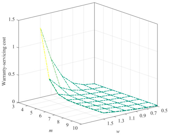
Figure 2.
The influences of and on costs.
Figure 2 shows that when is given, the increase in reduces the warranty-servicing cost of the RFRRW to a constant, which is the warranty-servicing cost of the CFRW (see Equation (3)); for a given , the increase in increases the warranty-servicing cost of the RFRRW.
Obviously, the increasing change and the minimum value in Proposition 1 do not appear in Figure 2. To illustrate the increasing change and the minimum value, the , , , and are plotted in Figure 3. Figure 3 shows that the minimum value exists, and the increasing change exists as well. These verify some of the terms in Proposition 1. , , , and are plotted in Figure 4. As shown in Figure 4, when is given, the increase in makes the warranty-servicing cost of the RFRRW increase to a constant, which belongs to the increasing change in Proposition 1.
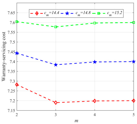
Figure 3.
The existence of the minimum value.
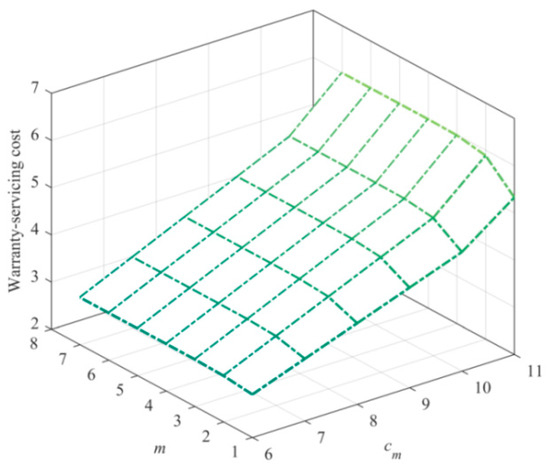
Figure 4.
The effects of and on costs.
4.1.2. Sensitivity Analysis of the 2DRFRRWF
Using , , , , and , Table 1 explores the influences of and on the warranty-servicing cost of the 2DRFRRWF and the relationships between the warranty-servicing costs of the 2DRFRRWF and CRFRRW. Table 1 shows that when is given, the increase in makes the warranty-servicing cost of the 2DRFRRWF decrease to a constant, which is the warranty-servicing cost of the RFRRW (see Equation (12)); increases the warranty-servicing cost of the 2DRFRRWF, which is similar to Figure 2.

Table 1.
The influences of and on the cost.
To explore how and influence the warranty-servicing cost of the 2DRFRRWF, , , , , and are plotted in Figure 5. Figure 5 shows that when is smaller, the warranty-servicing cost of the 2DRFRRWF decreases to a constant; when is greater, the warranty-servicing cost of the 2DRFRRWF decreases to a minimum value and then increases to a constant, which is the warranty-servicing cost of the 2DFRWF. These verify some of the terms in Proposition 3.
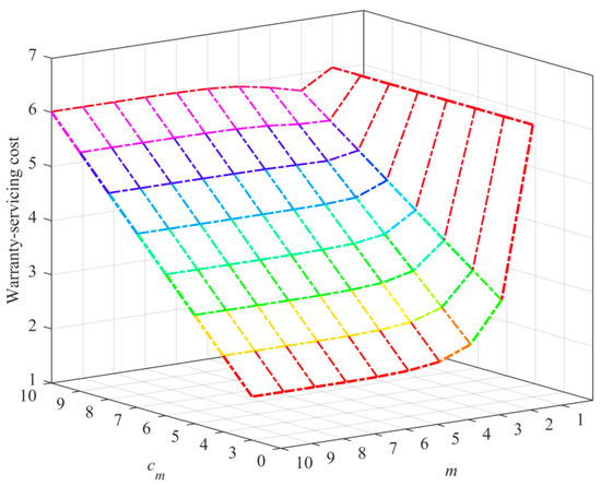
Figure 5.
The influences of and on the cost.
4.1.3. Sensitivity Analysis of the 2DRFRRWL
To explore how and influence the warranty-servicing cost of the 2DRFRRWL, , , , , and are plotted in Figure 6. Figure 6 shows that when is given, the increase of makes the warranty-servicing cost of the 2DRFRRWL increase to a constant, which is the warranty-servicing cost of the RFRRW (see Equation (25)); when is given, the increase in makes the warranty-servicing cost of the 2DRFRRWL increase, which is similar to Figure 2 and Table 1.
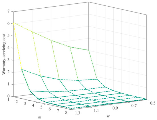
Figure 6.
The effects of and on the cost.
To explore how and influence the warranty-servicing cost of the 2DRFRRWL, , , , , and are plotted in Figure 7.
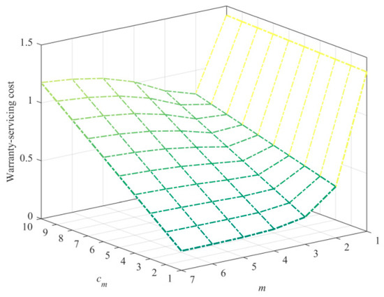
Figure 7.
The effects of and on the cost.
Figure 7 shows that when is smaller, the increase in makes the warranty-servicing cost of the 2DRFRRWL decrease to a constant, which is the warranty-servicing cost of the 2DFRWL (see Equation (29)); when is greater, the warranty-servicing cost of the 2DRFRRWL decreases to a minimum value and then increases to a constant, which is the warranty-servicing cost of the 2DFRWL. These results verify Proposition 5.
4.2. Sensitivity Analysis of the Post-Warranty Replacement Models
4.2.1. Sensitivity Analysis of the Replacement First Model
To verify that the optimal BRRF exists, , , , , and are plotted in Figure 8. As shown in Figure 8, the optimal number of mission cycles and the optimal planned time exist, and thus, the optimal BRRF exists uniquely.
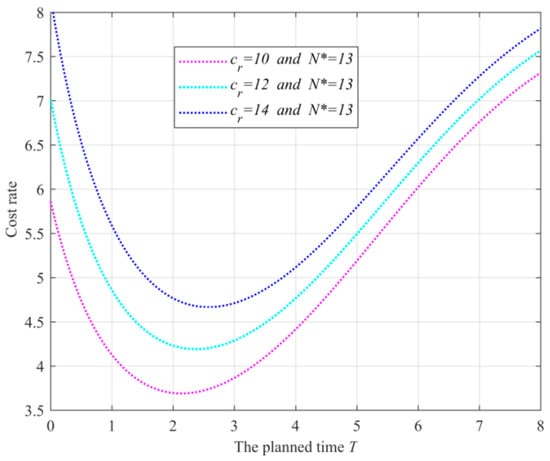
Figure 8.
Verification of the optimal BRRF.
To explore the influences of and on the optimal BRRF, Table 2 has been provided using , , , , and .
Table 2.
The influences of and on the optimal BRRF.
As shown in Table 2, ① for a given , the optimal average cost rate increases with respect to , and the optimal number of mission cycles is non-decreasing; ② for a given , the optimal average cost rate decreases with respect to , and the optimal number of mission cycles is non-decreasing. The former implies that the increase in can enhance the optimal average cost rate and that the optimal planned time can be lengthened; the latter implies that the increase in can reduce the optimal average cost rate and shorten the optimal planned time . These results indicate that consumers obtain either longer durations of warranty coverage or a longer duration of replacement coverage, but not both simultaneously.
4.2.2. Sensitivity Analysis of the Replacement Last Model
To verify whether the optimal BRRL exists, , , , , , and are plotted in Figure 9. As shown in Figure 9, the optimal number of mission cycles and the optimal planned time exist, and thus, the optimal BRRL exists uniquely.
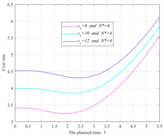
Figure 9.
Verification of the optimal BRRL.
To explore the influences of and on the optimal BRRL, Table 3 has been provided using , , , , and . As shown in Table 3, ① for a given , the optimal average cost rate increases with respect to , and the optimal number of mission cycles is also non-decreasing, which are the same as the changes in Table 2; ② for a given , the optimal average cost rate decreases with respect to , and the optimal number of mission cycles is also non-decreasing, which are the same as the changes in Table 2. The former implies that the increase in can enhance the optimal average cost rate and lengthen the optimal planned time ; the latter implies that the increase in can reduce the optimal average cost rate but cannot lengthen the optimal planned time . These results signal that the consumer only obtains either longer durations of warranty coverage or a longer duration of replacement coverage and cannot obtain both simultaneously, which is similar to the insights in Table 2.
Table 3.
The influences of and on the optimal BRRL.
4.3. Performance Analysis of the Presented Strategies/Models
4.3.1. Performance Analysis of Renewable Warranty Strategies
An ideal regulation for comparing the effectiveness of different warranty strategies would be that changes in the warranty-servicing cost and time are inversely proportional. However, according to Equations (22) and (24), the warranty-servicing cost and time uniformly increase, making it challenging to conduct an analytical comparison of performances using these strategies. The warranty-servicing time and cost are measured in different units, so it is necessary to convert both measurements to the same unit in order to compare the proposed solutions. By standardizing the measurements to a common unit, Shang et al. [47] have proposed a comparative methodology for evaluating the performances of the 2DRFRRWF and 2DRFRRWL from a manufacturer’s perspective. The cost measures, denoted as and , are associated with the 2DRFRRWF and 2DRFRRWL, respectively, when the time measures (i.e., comparison cycles) are equal. Taking inspiration from these approaches, Table 4 has been provided to assess the effectiveness of the warranty strategies, wherein , , , , , and .
Table 4.
Performance comparison of 2DRFRRWF and 2DRFRRWL.
Table 4 shows that when the time measures are equal, the cost measure related to the 2DRFRRWF is less than the cost measure related to the 2DRFRRWL, i.e., . Such an inequation signals that from the perspective of manufacturers, the 2DRFRRWF is superior to the 2DRFRRWL, because the manufacturers can absorb less warranty-servicing costs.
This result is obtained when the requirement to enhance the sales volume of products is ignored. If the objective is to boost the sales volume, then it is advisable to compare the time measures instead of the cost measures, because consumers tend to prefer warranties with longer servicing times or a greater coverage area. According to the comparison method presented by Shang et al. [47], when the cost measures are equal, the time measures related to the 2DRFRRWF and 2DRFRRWL are and , respectively. According to Table 4, it is obvious that the 2DRFRRWL is superior to the 2DRFRRWF. This comparison is performed from the viewpoints of consumers/users.
By extending the comparison method, the performances among the RFRRW, 2DRFRRWF, and 2DRFRRWL are numerically compared as well, which is no longer presented here.
4.3.2. Performance Analysis of Replacement Models
The performances of the BRRF and BRRL can be numerically compared by standardizing the measurements to a common unit, similar to comparing the performances of the 2DRFRRWF and 2DRFRRWL.
The cost measures, denoted as and , are associated with the BRRF and BRRL, respectively, assuming equal time measures. In the scenario where both time measures are equal, Table 5 presents a comparative analysis of the performances between BRRF and BRRL, where , , , , , and .
Table 5.
Performance comparison of the BRRF and BRRL.
As shown in Table 5, the cost measure related to the BRRF is less than the cost measure related to the BRRL, i.e., . This inequation signals that the BRRF is superior to the BRRL.
5. Conclusions
The number of failures is one of the factors affecting the dynamical changes in the reliability of self-announcing failure products subject to mission cycles. In view of this, this paper presents three renewable warranty strategies considering the failure number for managing the warranty-stage reliability of self-announcing failure products subject to mission cycles. The first renewable warranty strategy is proposed using the warranty period as a unique warranty limitation and the limited failure number as the replacement threshold during warranty coverage, which is named a renewable free-repair–replacement warranty (RFRRW). In the case of using a limited failure number as the replacement threshold, the second renewable warranty strategy is proposed using limited mission cycles and the warranty period as two warranty limitations, which is named a two-dimensional, renewable free-repair–replacement warranty first (2DRFRRWF), because ‘whichever occurs first’ is used to restrict the warranty region formed by limited mission cycles and the warranty period. By revising ‘whichever occurs first’ to ‘whichever occurs last’, the third renewable warranty strategy is presented, which is called a two-dimensional, renewable free-repair–replacement warranty (2DRFRRWL). All presented renewable warranties are modeled from the viewpoints of cost and time measures, and respective insights that guide decision making are obtained by means of cost and time measures. A numerical analysis of these three strategies was performed to verify the analytical insights and explore how other parameters affect them.
The life cycle of self-announcing failure products subject to mission cycles can be divided into warranty and post-warranty stages using the boundaries of the 2DRFRRWF region as symmetrical points. In this scenario, two post-warranty replacements considering the failure number are defined and modeled to manage the post-warranty reliability of self-announcing failure products subject to mission cycles, which are named the trivariate random replacement first (TRRF) and the trivariate random replacement last (TRRL), because three decision variables are considered, and ‘whichever occurs first and last’ is used to restrict respective replacement regions. By setting the parameter values of decision variables, some of the variants of both are presented, such as a bivariate random replacement first (BRRF), a bivariate random discrete replacement first (BRDRF), a bivariate random replacement last (BRRL), and a bivariate random discrete replacement last (BRDRL). Taking some post-warranty replacements as representatives, a numerical analysis is performed to verify the existence of optimal models and explore how other parameters affect them.
By employing a numerical analysis, valuable insights have been derived, encompassing a wide range of findings and discoveries:
- The renewable warranties introduced in this study offer advantages over the respective free-repair warranty (FRW) by reducing the warranty-servicing cost and extending the duration of the warranty coverage;
- Manufacturers tend to prefer the 2DRFRRWF, as it leads to reduced costs associated with warranty services. Conversely, consumers are more inclined towards favoring the 2DRFRRWL due to its extended duration for warranty servicing;
- The consumers are given the choice to opt for either an extended warranty coverage duration or a longer duration of replacement coverage; however, they cannot avail both simultaneously.
In this paper, three renewable warranties considering the failure number are proposed and modeled to manage the warranty-stage reliability of self-announcing failure products subject to mission cycles. Among them, the last two strategies will trigger warranty unfairness, because multidimensional warranty strategies can produce different warranty-servicing times. Although some works have studied methods to remove the unfairness of the warranty of multidimensional warranty strategies, the related authors have confined their focus to removing the unfairness of the warranty at the warranty-expiring stage and ignored removing the unfairness of the warranty at the warranty-opening stage or in the warranty process. Therefore, researching methods to remove warranty unfairness during these two stages is a future topic.
Author Contributions
Conceptualization, L.S. and L.Y.; methodology, L.S.; software, C.L.; validation, J.C.; formal analysis, J.C.; investigation, L.S.; resources, B.L.; writing—original draft preparation, L.S.; writing—review and editing, L.Y.; visualization, C.L. supervision, L.Y.; project administration, C.L.; funding acquisition, B.L. All authors have read and agreed to the published version of the manuscript.
Funding
This article was supported by the National Natural Science Foundation of China (Nos. 72161025 and 72271169).
Data Availability Statement
The authors confirm that the data supporting the findings of this study are available within the article.
Acknowledgments
The authors sincerely thank all unknown reviewers for their valuable suggestions and helpful comments that have led to the present form of the original manuscript.
Conflicts of Interest
The authors declare no conflicts of interest.
Appendix A
Obviously, . Using , it is obvious for to hold.
Appendix B. The Proof of Proposition 1
Obviously, decreases with respect to , whose minimum and maximum values are 0 and , respectively; is increasing with respect to , whose minimum and maximum values are 0 and , respectively. These characteristics signal that the curves of the function , with respect to , and the function , with respect to , intersect. The intersection points of both, satisfying , can make the function , with respect to , reach its minimum value. On the right side of the intersection point, the function is increasing with respect to , satisfying ; on the left side of the intersection point, the function is decreasing with respect to , satisfying . Let ; then, by means of operations, three mathematical relationships can be obtained: , , and .
Appendix C. The Proof of Proposition 2
Because and are increasing with respect to , by means of the monotonicity rule of the compound function, the function is decreasing with respect to , and its maximum and minimum values are and , respectively.
References
- Zhang, T.; Xie, M. On the upper truncated Weibull distribution and its reliability implications. Reliab. Eng. Syst. Saf. 2011, 96, 194–200. [Google Scholar] [CrossRef]
- Ducros, F.; Pamphile, P. Bayesian estimation of Weibull mixture in heavily censored data setting. Reliab. Eng. Syst. Saf. 2018, 180, 453–462. [Google Scholar] [CrossRef]
- Song, K.; Cui, L. A common random effect induced bivariate gamma degradation process with application to remaining useful life prediction. Reliab. Eng. Syst. Saf. 2022, 219, 108200. [Google Scholar] [CrossRef]
- Wang, H.; Liao, H.; Ma, X.; Bao, R. Remaining useful life prediction and optimal maintenance time determination for a single unit using isotonic regression and gamma process model. Reliab. Eng. Syst. Saf. 2021, 210, 107504. [Google Scholar] [CrossRef]
- Ye, Z.S.; Xie, M. Stochastic modelling and analysis of degradation for highly reliable products. Appl. Stoch. Models Bus. Ind. 2015, 31, 16–32. [Google Scholar] [CrossRef]
- Qiu, Q.; Cui, L. Gamma process based optimal mission abort policy. Reliab. Eng. Syst. Saf. 2019, 190, 106496. [Google Scholar] [CrossRef]
- van Noortwijk, J.M.; van der Weide, J.A.; Kallen, M.J.; Pandey, M.D. Gamma processes and peaks-over-threshold distributions for time-dependent reliability. Reliab. Eng. Syst. Saf. 2007, 92, 1651–1658. [Google Scholar] [CrossRef]
- Zhang, S.; Zhai, Q.; Li, Y. Degradation modeling and RUL prediction with Wiener process considering measurable and unobservable external impacts. Reliab. Eng. Syst. Saf. 2023, 231, 109021. [Google Scholar] [CrossRef]
- Zhou, S.; Tang, Y.; Xu, A. A generalized Wiener process with dependent degradation rate and volatility and time-varying mean-to-variance ratio. Reliab. Eng. Syst. Saf. 2021, 216, 107895. [Google Scholar] [CrossRef]
- Ye, Z.S.; Chen, N.; Shen, Y. A new class of Wiener process models for degradation analysis. Reliab. Eng. Syst. Saf. 2015, 139, 58–67. [Google Scholar] [CrossRef]
- Mukhopadhyay, K.; Liu, B.; Bedford, T.; Finkelstein, M. Remaining lifetime of degrading systems continuously monitored by degrading sensors. Reliab. Eng. Syst. Saf. 2023, 231, 109022. [Google Scholar] [CrossRef]
- Lu, B.; Chen, Z.; Zhao, X. Data-driven dynamic adaptive replacement policy for units subject to heterogeneous degradation. Comput. Ind. Eng. 2022, 171, 108478. [Google Scholar] [CrossRef]
- Guo, B.; Wang, B.X.; Xie, M. A study of process monitoring based on inverse Gaussian distribution. Comput. Ind. Eng. 2014, 76, 49–59. [Google Scholar] [CrossRef]
- Wang, Y.; Liu, Y.; Chen, J.; Li, X. Reliability and condition-based maintenance modeling for systems operating under performance-based contracting. Comput. Ind. Eng. 2020, 142, 106344. [Google Scholar] [CrossRef]
- Chen, C.K.; Lo, C.C.; Weng, T.C. Optimal production run length and warranty period for an imperfect production system under selling price dependent on warranty period. Eur. J. Oper. Res. 2017, 259, 401–412. [Google Scholar] [CrossRef]
- Ye, Z.; Murthy, D.N.P.; Xie, M.; Tang, L. Optimal burn-in for repairable products sold with a two-dimensional warranty. IIE Trans. 2013, 45, 164–176. [Google Scholar] [CrossRef]
- Qiao, P.; Shen, J.; Zhang, F.; Ma, Y. Optimal warranty policy for repairable products with a three-dimensional renewable combination warranty. Comput. Ind. Eng. 2022, 168, 108056. [Google Scholar] [CrossRef]
- Wang, X.; Zhao, X.; Liu, B. Design and pricing of extended warranty menus based on the multinomial logit choice model. Eur. J. Oper. Res. 2020, 287, 237–250. [Google Scholar] [CrossRef]
- Su, P.; Jiang, W.; Wei, L.; Wang, X.L. A new cost-sharing preventive maintenance program under two-dimensional warranty. Int. J. Prod. Econ. 2022, 254, 108580. [Google Scholar]
- Liu, B.; Wu, J.; Xie, M. Cost analysis for multi-component system with failure interaction under renewing free-replacement warranty. Eur. J. Oper. Res. 2015, 243, 874–882. [Google Scholar] [CrossRef]
- Wang, X.; He, K.; He, Z.; Li, L.; Xie, M. Cost analysis of a piece-wise renewing free replacement warranty policy. Comput. Ind. Eng. 2019, 135, 1047–1062. [Google Scholar] [CrossRef]
- Rao, B.M. Cumulative free replacement warranty with phase type lifetime distributions. Comput. Ind. Eng. 2021, 162, 107771. [Google Scholar] [CrossRef]
- Wang, X.; Xie, M.; Li, L. On optimal upgrade strategy for second-hand multi-component systems sold with warranty. Int. J. Prod. Res. 2019, 57, 847–864. [Google Scholar] [CrossRef]
- Shang, L.; Si, S.; Sun, S.; Jin, T. Optimal warranty design and post-warranty maintenance for products subject to stochastic degradation. IISE Trans. 2018, 50, 913–927. [Google Scholar] [CrossRef]
- Zhang, N.; Fouladirad, M.; Barros, A. Evaluation of the warranty cost of a product with type III stochastic dependence between components. Appl. Math. Model. 2018, 59, 39–53. [Google Scholar] [CrossRef]
- Liu, P.; Wang, G.; Su, P. Optimal replacement strategies for warranty products with multiple failure modes after warranty expiry. Comput. Ind. Eng. 2021, 153, 107040. [Google Scholar] [CrossRef]
- Park, M.; Pham, H. Cost models for age replacement policies and block replacement policies under warranty. Appl. Math. Model. 2016, 40, 5689–5702. [Google Scholar] [CrossRef]
- Park, M.; Jung, K.M.; Park, D.H. Optimization of periodic preventive maintenance policy following the expiration of two-dimensional warranty. Reliab. Eng. Syst. Saf. 2018, 170, 1–9. [Google Scholar] [CrossRef]
- Shang, L.; Si, S.; Cai, Z. Optimal maintenance–replacement policy of products with competing failures after expiry of the warranty. Comput. Ind. Eng. 2016, 98, 68–77. [Google Scholar] [CrossRef]
- Liu, P.; Wang, G. Generalized non-renewing replacement warranty policy and an age-based post-warranty maintenance strategy. Eur. J. Oper. Res. 2023, 311, 567–580. [Google Scholar] [CrossRef]
- Shang, L.; Qiu, Q.; Wang, X. Random periodic replacement models after the expiry of 2D-warranty. Comput. Ind. Eng. 2022, 164, 107885. [Google Scholar] [CrossRef]
- Wang, J.; Qiu, Q.; Wang, H. Joint optimization of condition-based and age-based replacement policy and inventory policy for a two-unit series system. Reliab. Eng. Syst. Saf. 2021, 205, 107251. [Google Scholar] [CrossRef]
- Wang, J.; Qiu, Q.; Wang, H.; Lin, C. Optimal condition-based preventive maintenance policy for balanced systems. Reliab. Eng. Syst. Saf. 2021, 211, 107606. [Google Scholar] [CrossRef]
- Chen, Y.; Qiu, Q.; Zhao, X. Condition-based opportunistic maintenance policies with two-phase inspections for continuous-state systems. Reliab. Eng. Syst. Saf. 2022, 228, 108767. [Google Scholar] [CrossRef]
- Qiu, Q.; Cui, L.; Gao, H. Availability and maintenance modelling for systems subject to multiple failure modes. Comput. Ind. Eng. 2017, 108, 192–198. [Google Scholar] [CrossRef]
- Qiu, Q.; Cui, L.; Shen, J. Availability and maintenance modeling for systems subject to dependent hard and soft failures. Appl. Stoch. Models Bus. Ind. 2018, 34, 513–527. [Google Scholar] [CrossRef]
- Qiu, Q.; Cui, L.; Kong, D. Availability and maintenance modeling for a two-component system with dependent failures over a finite time horizon. Proc. Inst. Mech. Eng. Part O J. Risk Reliab. 2018, 233, 200–210. [Google Scholar] [CrossRef]
- Qiu, Q.; Cui, L. Availability analysis for general repairable systems with repair time threshold. Commun. Stat.-Theory Methods 2019, 48, 628–647. [Google Scholar] [CrossRef]
- Qiu, Q.; Cui, L.; Shen, J. Availability analysis and maintenance modelling for inspected Markov systems with down time threshold. Qual. Technol. Quant. Manag. 2019, 16, 478–495. [Google Scholar] [CrossRef]
- Qiu, Q.; Cui, L.; Kong, D. Availability analysis and optimal inspection policy for systems with neglected down time. Commun. Stat.—Theory Methods 2019, 48, 2787–2809. [Google Scholar] [CrossRef]
- Qiu, Q.; Cui, L. Availability analysis for periodically inspected systems subject to multiple failure modes. Int. J. Syst. Sci. Oper. Logist. 2019, 6, 258–271. [Google Scholar] [CrossRef]
- Qiu, Q.; Cui, L. Optimal mission abort policy for systems subject to random shocks based on virtual age process. Reliab. Eng. Syst. Saf. 2019, 189, 11–20. [Google Scholar] [CrossRef]
- Qiu, Q.; Cui, L.; Dong, Q. Preventive maintenance policy of single-unit systems based on shot-noise process. Qual. Relia. Eng. Int. 2019, 35, 550–560. [Google Scholar] [CrossRef]
- Zhao, X.; Chai, X.; Cao, S.; Qiu, Q. Dynamic loading and condition-based maintenance policies for multi-state systems with periodic inspection. Reliab. Eng. Syst. Saf. 2023, 240, 109586. [Google Scholar] [CrossRef]
- Yang, L.; Wei, F.; Qiu, Q. Mission risk control via joint optimization of sampling and abort decisions. Risk Anal. 2024, 44, 666–685. [Google Scholar] [CrossRef]
- Peng, R.; He, X.; Zhong, C.; Kou, G.; Xiao, H. Preventive maintenance for heterogeneous parallel systems with two failure modes. Reliab. Eng. Syst. Saf. 2022, 220, 108310. [Google Scholar] [CrossRef]
- Shang, L.; Liu, B.; Qiu, Q.; Yang, L.; Du, Y. Designing warranty and maintenance policies for products subject to random working cycles. Reliab. Eng. Syst. Saf. 2023, 234, 109187. [Google Scholar] [CrossRef]
Disclaimer/Publisher’s Note: The statements, opinions and data contained in all publications are solely those of the individual author(s) and contributor(s) and not of MDPI and/or the editor(s). MDPI and/or the editor(s) disclaim responsibility for any injury to people or property resulting from any ideas, methods, instructions or products referred to in the content. |
© 2024 by the authors. Licensee MDPI, Basel, Switzerland. This article is an open access article distributed under the terms and conditions of the Creative Commons Attribution (CC BY) license (https://creativecommons.org/licenses/by/4.0/).