Bayesian Inference for the Gamma Zero-Truncated Poisson Distribution with an Application to Real Data

Abstract

This article presents Bayesian estimation methods applied to the gamma zero-truncated Poisson (GZTP) and the complementary gamma zero-truncated Poisson (CGZTP) distributions, encompassing both one-parameter and two-parameter models. These distributions are notably flexible and useful for modeling lifetime data. In the one-parameter model case, the Jeffreys prior is mathematically derived. The use of informative and noninformative priors, combined with the random walk Metropolis algorithm within a Bayesian framework, generates samples from the posterior distributions. Bayesian estimators’ effectiveness is examined through extensive simulation studies, in comparison with the maximum likelihood method. Results indicate that Bayesian estimators provide more precise parameter estimates, even with smaller sample sizes. Furthermore, the study and comparison of the coverage probabilities (CPs) and average lengths (ALs) of the credible intervals with those from Wald intervals suggest that Bayesian credible intervals typically yield shorter ALs and higher CPs, thereby demonstrating the effectiveness of Bayesian inference in the context of GZTP and CGZTP distributions. Lastly, Bayesian inference is applied to real data.

1. Introduction

The gamma zero-truncated Poisson (GZTP) and complementary gamma zero-truncated Poisson (CGZTP) distributions hold significant importance in statistical modeling, particularly for lifetime data exhibiting nonmonotonic hazard functions. The GZTP distribution provides a flexible model for phenomena where an event is guaranteed to occur, effectively handling datasets where zero counts are inapplicable. This makes it ideal for reliability analyses where the time to first failure is of interest. The CGZTP further extends this utility by modeling the bathtub-shaped hazard function, which is characterized by an initial decrease, followed by a constant rate, and then an increase. Such a capability to fit a bathtub hazard function makes the CGZTP a robust tool for complex survival data, overcoming the limitations of traditional models such as the gamma distribution.

The GZTP distribution, introduced by Niyomdecha et al. [1], is derived from compounding the gamma and zero-truncated Poisson distributions using the minimum function. Consider a collection of N independent and identically distributed random variables $X_1,X_2,\dots ,X_N$, each following a gamma distribution with a probability density function $f(x;\alpha ,\beta )$ defined as $f(x;\alpha ,\beta )={\beta }^{\alpha }{x}^{\alpha -1}{e}^{-\beta x}/\Gamma \left(\alpha \right),x>0$, where $\alpha >0$ is a shape parameter and $\beta >0$ is a rate parameter. The variable N follows a zero-truncated Poisson distribution, given by: $P(N=n)=e^{-\lambda }{\lambda }^n/n!\left(1-e^{-\lambda }\right), n=1,2,\dots$, and $\lambda >0$. Assuming X and N are independent, Z is defined as the minimum of $X_1,X_2,\dots ,X_N$. The probability density function (pdf) of the GZTP distribution is denoted as

$$f_{GZTP}(z;\lambda ,\alpha ,\beta )=\left(\frac{\lambda {\beta }^{\alpha }{z}^{\alpha -1}{e}^{-\lambda -\beta z}}{\Gamma \left(\alpha \right)\left(1-e^{-\lambda }\right)}\right)\exp \left[\lambda \left(\frac{\Gamma \left(\alpha ,\beta z\right)}{\Gamma \left(\alpha \right)}\right)\right],\hspace{1em}z>0,\hspace{0.17em}\lambda >0,\alpha >0,\beta >0,$$

(1)

where $\Gamma \left(\alpha ,\beta z\right)=$${\displaystyle \underset{\beta z}{\overset{\infty }{\int }}{t}^{\alpha -1}{e}^{-t}dt}$ is the upper incomplete gamma function. The CGZTP distribution utilizes the same compounding principle as the GZTP but employs the maximum function instead [2]. Consider Y to be the maximum of $X_1,X_2,\dots ,X_N$. The pdf for the CGZTP distribution is then given as follows:

$$f_{CGZTP}(y;\lambda ,\alpha ,\beta )=\left(\frac{\lambda {\beta }^{\alpha }{y}^{\alpha -1}{e}^{-\lambda -\beta y}}{\Gamma \left(\alpha \right)\left(1-e^{-\lambda }\right)}\right)\exp \left[\lambda \left(1-\frac{\Gamma (\alpha ,\beta y)}{\Gamma \left(\alpha \right)}\right)\right],\hspace{0.17em} y>0,\lambda >0,\alpha >0,\beta >0.$$

(2)

These distributions exhibit flexible shapes of distribution functions, as shown in Figure 1. Previous studies have covered inferential procedures for the parameters of the GZTP and CGZTP distributions. Niyomdecha et al. [1] employed maximum likelihood estimation (MLE) to estimate GZTP parameters and then examine their asymptotic properties, while the MLEs and asymptotic confidence intervals for CGZTP parameters were discussed by Niyomdecha and Srisuradetchai [2]. The MLEs exhibited accurate estimations, and the confidence interval achieved the nominal coverage probability in the case of a large sample size. Several studies have been conducted on compound distributions using Bayesian methods. Xu et al. [3] investigated Bayesian estimators of Exponential-Poisson (EP) parameters by employing general noninformation prior distributions under symmetric and asymmetric loss functions. Yan et al. [4] determined the Bayesian estimators of the parameters in the EP distribution under general entropy, LINEX, and a scaled squared loss function based on type-II censoring. In a study conducted by Pathak et al. [5], the Bayesian estimators of Weibull–Poisson (WP) parameters were obtained by assuming that these parameters follow independently distributed prior distributions.

Figure 1. Probability density functions of GZTP (left) and CGZTP (Right) for various parameter sets $\theta =(\lambda ,\alpha ,\beta )$.

The loss function is instrumental in measuring how much an estimated parameter value deviates from its true value. The squared error loss function, a symmetric loss function, is commonly used in practice, especially when overestimation and underestimation are equally problematic [6,7]. Elbatal et al. [8] addressed parameter estimation for the Nadarajah–Haghighi distribution with progressive Type-1 censoring, employing the squared error loss function to produce Bayes estimates and credible intervals for maximum posterior density. Eliwa et al. [9] utilized balanced linear exponential and general entropy loss functions to estimate parameters for the new Weibull-Pareto distribution. Similarly, Abdel-Aty et al. [10] applied squared error, LINEX, and general entropy loss functions for future failure times in a joint type-II censored sample from multiple exponential populations.

In many studies, the posterior distributions often become complicated and cannot be simplified into any closed form. The samples were obtained from the posteriors using a Markov Chain Monte Carlo (MCMC) method, such as the Gibbs sampler (see [11]) and the Metropolis–Hastings algorithm (see [12]). Additionally, a summary of the predicted posteriors is provided based on a sample-based approach. The MCMC based on Metropolis–Hastings algorithms was used in [13] to estimate the unknown parameters of the alpha-power Weibull distribution under Type II hybrid censoring. In [14], the parameters of the unit-log-logistic distribution were estimated using a Bayesian approach. Noninformative priors were used, and samples from the joint posterior distribution were obtained using the random walk Metropolis algorithm. El-Sagheer et al. [15] employed Gibbs sampling to estimate the parameters for an asymmetric distribution and various lifetime indices, including reliability and hazard rate functions.

It is widely regarded that the conjugate prior for the Poisson parameter and the gamma rate parameter follow a gamma distribution. However, there is no proper conjugate prior for the gamma shape parameter [16,17]. Several papers explore Bayesian inference for estimating the parameters of the gamma distribution. Naji and Rasheed [18] derived Bayes estimators for the shape and scale parameters of the gamma distribution using the precautionary loss function. They assumed gamma and exponential priors for the shape and scale parameters, respectively, to represent prior information. Moala et al. [19] studied various noninformative priors, including Jeffreys prior, reference prior, maximal data information prior, Tibshirani prior, and a novel prior based on the copula method. Additionally, Pradhan and Kundu [20] assumed that the scale parameter follows a gamma distribution prior, while the shape parameter follows a log-concave distribution prior.

The existing literature has not addressed Bayesian inference on parameters of the GZTP and CGZTP) distributions. While Niyomdecha et al. [1] and Niyomdecha and Srisuradetchai [2] have conducted MLE and Wald’s interval analyses, their findings suggest that the mean square errors of MLEs remain high and that Wald’s interval coverage probabilities are below the nominal level for small sample sizes. This study, therefore, seeks to explore Bayesian inference for the GZTP and CGZTP distributions.

This paper is structured as follows: Section 2 delves into maximum likelihood estimation along with the corresponding interval estimation, which will be compared with the Bayesian credible interval. Section 3 elaborates on the prior and posterior distributions, estimation procedures based on the squared error loss function, and the application of the random walk Metropolis algorithm for simulating posterior samples. Simulation studies, which are conducted for scenarios involving one and two unknown parameters within both GZTP and CGZTP distributions, are presented in Section 4. Section 5 demonstrates two example applications using real data. Finally, the paper concludes with a discussion in Section 6.

2. Maximum Likelihood Estimation

Let $Z_1,Z_2,\dots ,Z_n$ be random samples from a GZTP distribution and $Y_1,Y_2,\dots ,Y_n$ be random samples from a CGZTP distribution. The likelihood functions based on the observed random sample of size $n$ will be as follows:

$$L_{GZTP}\left(\lambda ,\alpha ,\beta |z\right)={\left(\frac{\lambda e^{-\lambda }}{1-e^{-\lambda }}\right)}^n\left(\frac{{\beta }^{n\alpha }}{{\left(\Gamma \left(\alpha \right)\right)}^n}\right){\left({\displaystyle \prod _{i=1}^n{z}_i}\right)}^{\alpha -1}\exp \left[-\beta \left({\displaystyle \sum _{i=1}^n{z}_i}\right)+\frac{\lambda }{\Gamma \left(\alpha \right)}{\displaystyle \sum _{i=1}^n\Gamma \left(\alpha ,\beta z_i\right)}\right],$$

(3)

$$L_{CGZTP}\left(\lambda ,\alpha ,\beta |y\right)={\left(\frac{\lambda }{1-e^{-\lambda }}\right)}^n\left(\frac{{\beta }^{n\alpha }}{{\left(\Gamma \left(\alpha \right)\right)}^n}\right){\left({\displaystyle \prod _{i=1}^n{y}_i}\right)}^{\alpha -1}\exp \left[-\beta \left({\displaystyle \sum _{i=1}^n{y}_i}\right)-\frac{\lambda }{\Gamma \left(\alpha \right)}{\displaystyle \sum _{i=1}^n\Gamma \left(\alpha ,\beta y_i\right)}\right].$$

(4)

The corresponding log-likelihood function of the GZTP distribution is

$$\begin{array}{l}{l}_{GZTP}\left(\lambda ,\alpha ,\beta |z\right)=n\left(\log \lambda -\lambda -\log \left(1-e^{-\lambda }\right)\right)+n\alpha \log \beta -n\log \Gamma \left(\alpha \right)+\left(\alpha -1\right){\displaystyle \sum _{i=1}^n\log z_i}\\ \hspace{1em}\hspace{1em}\hspace{1em}-\beta \left({\displaystyle \sum _{i=1}^n{z}_i}\right)+\frac{\lambda }{\Gamma \left(\alpha \right)}{\displaystyle \sum _{i=1}^n\Gamma \left(\alpha ,\beta z_i\right)},\end{array}$$

(5)

and the log-likelihood function of the CGZTP distribution is

$$\begin{array}{l}{l}_{CGZTP}\left(\lambda ,\alpha ,\beta |y\right)=n\left(\log \lambda -\log \left(1-e^{-\lambda }\right)\right)+n\alpha \log \beta -n\log \Gamma \left(\alpha \right)+\left(\alpha -1\right){\displaystyle \sum _{i=1}^n\log y_i}\\ \hspace{1em}\hspace{1em}\hspace{1em}-\beta \left({\displaystyle \sum _{i=1}^n{y}_i}\right)-\frac{\lambda }{\Gamma \left(\alpha \right)}{\displaystyle \sum _{i=1}^n\Gamma \left(\alpha ,\beta y_i\right)}.\end{array}$$

(6)

The maximum likelihood estimators of $\lambda$, $\alpha$ and $\beta$ for the GZTP and CGZTP distributions are obtained by maximizing (5) and (6). This process is accomplished by solving the first derivatives with respect to each parameter of the log-likelihood function. These first derivatives are difficult and complex to solve, making it impossible to find the MLE of $\lambda$, $\alpha$ and $\beta$ analytically. Consequently, numerical techniques such as the simulated annealing method are employed to estimate $\lambda$, $\alpha$ and $\beta$ that maximize the likelihood function.

The MLEs are asymptotically normally distributed with a multivariate normal (MVN) distribution given by

$${\left(\widehat{\lambda },\widehat{\alpha },\widehat{\beta }\right)}^{\prime }\sim MVN\left({\left(\lambda ,\alpha ,\beta \right)}^{\prime },I^{-1}\left(\lambda ,\alpha ,\beta \right)\right) \mathrm{as} n\to \infty ,$$

where $I\left(\lambda ,\alpha ,\beta \right)$ is the Fisher information matrix with element $I_{ij}=-𝜕l^2/𝜕{\mathit{\theta }}_i𝜕{\mathit{\theta }}_j,$ $i,j=1,2,3$ and $\mathit{\theta }=\left(\lambda ,\alpha ,\beta \right)$ [21]. The asymptotic variances of MLEs can be obtained from the inverse Fisher information matrix. Then, the corresponding $\left(1-\alpha \right)100\%$ Wald confidence intervals for ${\theta }_i$ are given by ${\widehat{\theta }}_i\pm z_{1-\alpha /2}\sqrt{{\widehat{I}}^{ii}}$, where ${\widehat{I}}^{ii}$ is the ii-th element of the inverse of $\left[I{\left(\widehat{\theta }\right)}^{-1}\right]$, i.e., ${\widehat{I}}^{ii}={\left[I{\left(\widehat{\theta }\right)}^{-1}\right]}_{ii}$ and $z_{1-\alpha /2}$ is the $(1-\alpha /2)$-th quantile of the standard normal [22].

3. Bayesian Estimation

This section presents the formulation of prior distributions for each parameter, acknowledging their independence, and the subsequent derivation of joint posterior distributions.

3.1. Prior and Posterior Distributions

3.1.1. Case 1: $\alpha$ and $\beta$ Are Unknown

To estimate the parameters for the GZTP or CGZTP distributions when $\alpha$ and $\beta$ are unknown but $\lambda$ is known, we assume that $\alpha$ and $\beta$ have priors $p_1(\cdot )$ and $p_2(\cdot )$, which correspond to $Gamma\left(a, b\right)$ and $Gamma\left(c, d\right)$, respectively, and they are independently distributed. The prior distributions for $\alpha$ and $\beta$ are obtained as follows:

$$p_1\left(\alpha ;a,b\right)=\frac{b^a{\alpha }^{a-1}{e}^{-b\alpha }}{\Gamma \left(a\right)} \mathrm{and} p_2\left(\beta ;c,d\right)=\frac{d^c{\beta }^{c-1}{e}^{-d\beta }}{\Gamma \left(c\right)},$$

where hyperparameters $\beta >0, c>0, d>0.$

Let $Z_1,Z_2,\dots ,Z_n$ be random samples from a GZTP distribution, so the joint posterior distribution given data $z=(z_1,z_2,\dots ,z_n)$ is as follows:

$$\begin{array}{l}{p}_{GZTP}\left(\alpha ,\beta |z\right)\\ \hspace{1em}\hspace{1em}\hspace{1em}\hspace{1em}\hspace{1em}=\frac{L\left(\alpha ,\beta ;z\right)p_1\left(\alpha \right)p_2\left(\beta \right)}{{\displaystyle \underset{0}{\overset{\infty }{\int }}{\displaystyle \underset{0}{\overset{\infty }{\int }}L\left(\alpha ,\beta ;z\right)p_1\left(\alpha \right)p_2\left(\beta \right)d\alpha d\beta }}}\\ \hspace{1em}\hspace{1em}\hspace{1em}\hspace{1em}\hspace{1em}\propto L\left(\alpha ,\beta ;z\right)p_1\left(\alpha \right)p_2\left(\beta \right)\\ \hspace{1em}\hspace{1em}\hspace{1em}\hspace{1em}\hspace{1em}\propto {\left(\frac{\lambda e^{-\lambda }}{1-e^{-\lambda }}\right)}^n\left(\frac{{\beta }^{n\alpha }}{{\left(\Gamma \left(\alpha \right)\right)}^n}\right){\left({\displaystyle \prod _{i=1}^n{z}_i}\right)}^{\alpha -1}\exp \left[-\beta \left({\displaystyle \sum _{i=1}^n{x}_i}\right)+\frac{\lambda }{\Gamma \left(\alpha \right)}{\displaystyle \sum _{i=1}^n\Gamma \left(\alpha ,\beta z_i\right)}\right]\\ \hspace{1em}\hspace{1em}\hspace{1em}\hspace{1em}\hspace{1em}\hspace{0.17em}\hspace{0.17em}\hspace{0.17em}\times \left(\frac{b^a{\alpha }^{a-1}{e}^{-b\alpha }}{\Gamma \left(a\right)}\right)\left(\frac{d^c{\beta }^{c-1}{e}^{-d\beta }}{\Gamma \left(c\right)}\right),\end{array}$$

and $Y_1,Y_2,\dots ,Y_n$ are the random samples from the CGZTP distribution, and the corresponding joint posterior distribution given data $y=(y_1,y_2,\dots ,y_n)$ is given by:

$$\begin{array}{l}{p}_{CGZTP}\left(\alpha ,\beta |y\right)\propto {\left(\frac{\lambda }{1-e^{-\lambda }}\right)}^n\left(\frac{{\beta }^{n\alpha }}{{\left(\Gamma \left(\alpha \right)\right)}^n}\right){\left({\displaystyle \prod _{i=1}^n{y}_i}\right)}^{\alpha -1}\exp \left[-\beta \left({\displaystyle \sum _{i=1}^n{y}_i}\right)-\frac{\lambda }{\Gamma \left(\alpha \right)}{\displaystyle \sum _{i=1}^n\Gamma \left(\alpha ,\beta y_i\right)}\right]\\ \hspace{1em}\hspace{1em}\hspace{1em}\hspace{1em}\hspace{1em}\hspace{1em}\times \left(\frac{b^a{\alpha }^{a-1}{e}^{-b\alpha }}{\Gamma \left(a\right)}\right)\left(\frac{d^c{\beta }^{c-1}{e}^{-d\beta }}{\Gamma \left(c\right)}\right).\\ \hspace{1em}\hspace{1em}\hspace{1em}\hspace{1em}\hspace{1em}\end{array}$$

The marginal posterior distributions of $\alpha$ and $\beta$ have no closed form; as a consequence, the MCMC method is employed to provide Bayesian estimation.

3.1.2. Case 2: $\lambda$ Is Unknown

Gamma Priors

To estimate parameter $\lambda$ for the GZTP or CGZTP when $\alpha$ and $\beta$ are known. Assuming that $\lambda$ has a prior $Gamma\left(m, n\right)$:

$$p_3\left(\lambda \right)=\frac{n^m{\lambda }^{m-1}{e}^{-n\lambda }}{\Gamma \left(m\right)},\lambda >0, m>0, n>0.$$

Let $Z_1,Z_2,\dots ,Z_n$ be random samples from a GZTP distribution. The corresponding posterior distribution, given data $z=(z_1,z_2,\dots ,z_n)$, is as follows:

$$\begin{array}{l}{p}_{GZTP}\left(\lambda |z\right)\propto L\left(\lambda ;z\right)p_3\left(\lambda \right)\\ \hspace{1em}\hspace{1em}\hspace{0.17em}\hspace{0.17em}={\left(\frac{\lambda e^{-\lambda }}{1-e^{-\lambda }}\right)}^n\left(\frac{{\beta }^{n\alpha }}{{\left(\Gamma \left(\alpha \right)\right)}^n}\right){\left({\displaystyle \prod _{i=1}^n{z}_i}\right)}^{\alpha -1}\exp \left[-\beta \left({\displaystyle \sum _{i=1}^n{z}_i}\right)+\frac{\lambda }{\Gamma \left(\alpha \right)}{\displaystyle \sum _{i=1}^n\Gamma \left(\alpha ,\beta z_i\right)}\right]\times \left(\frac{n^m{\lambda }^{m-1}{e}^{-n\lambda }}{\Gamma \left(m\right)}\right).\end{array}$$

Furthermore, let $Y_1,Y_2,\dots ,Y_n$ be random samples from a CGZTP distribution. The corresponding posterior distribution given data $y=(y_1,y_2,\dots ,y_n)$ is:

$$\begin{array}{l}{p}_{CGZTP}\left(\lambda |y\right)\propto L\left(\lambda ;y\right)p_3\left(\lambda \right)\\ \hspace{1em}\hspace{1em}\hspace{0.17em}\hspace{0.17em}\hspace{0.17em} ={\left(\frac{\lambda }{1-e^{-\lambda }}\right)}^n\left(\frac{{\beta }^{n\alpha }}{{\left(\Gamma \left(\alpha \right)\right)}^n}\right){\left({\displaystyle \prod _{i=1}^n{y}_i}\right)}^{\alpha -1}\exp \left[-\beta \left({\displaystyle \sum _{i=1}^n{y}_i}\right)-\frac{\lambda }{\Gamma \left(\alpha \right)}{\displaystyle \sum _{i=1}^n\Gamma \left(\alpha ,\beta y_i\right)}\right]\times \left(\frac{n^m{\lambda }^{m-1}{e}^{-n\lambda }}{\Gamma \left(m\right)}\right).\end{array}$$

Because the posterior distributions above are also complicated to derive analytically, MCMC is used to simulate samples from them.

Jeffreys Prior

Jeffreys prior is proposed as a widely known prior to represent a situation in which there is little information regarding the parameters. The Jeffreys prior for one parameter is proportional to the square root of the expected Fisher information [23]. From the likelihood functions in cases when $\alpha$ and $\beta$ are known, the associated gradients are:

$$\frac{𝜕l_{GZTP}\left(\lambda ;z\right)}{𝜕\lambda }=n\left(\frac{1}{\lambda }-1-\frac{e^{-\lambda }}{1-e^{-\lambda }}\right)+\frac{{\displaystyle \sum _{i=1}^n\Gamma \left(\alpha ,\beta z_i\right)}}{\Gamma \left(\alpha \right)},$$

(7)

$$\frac{𝜕l_{CGZTP}\left(\lambda ;y\right)}{𝜕\lambda }=n\left(\frac{1}{\lambda }-\frac{e^{-\lambda }}{1-e^{-\lambda }}\right)-\frac{{\displaystyle \sum _{i=1}^n\Gamma \left(\alpha ,\beta y_i\right)}}{\Gamma \left(\alpha \right)}.$$

(8)

By differentiating (7) and (8), the observed Fisher information values of $\lambda$ for the GZTP and CGZTP distributions are the same:

$$I_{GZTP}\left(\lambda \right)=I_{CGZTP}\left(\lambda \right)=\frac{n(1+e^{2\lambda }-e^{\lambda }({\lambda }^2+2))}{{\left(e^{\lambda }-1\right)}^2{\lambda }^2}$$

and the expected Fisher information is

$$J_{GZTP}\left(\lambda \right)=J_{CGZTP}\left(\lambda \right)=E\left[\frac{n(1+e^{2\lambda }-e^{\lambda }({\lambda }^2+2))}{{\left(e^{\lambda }-1\right)}^2{\lambda }^2}\right]=\frac{n(1+e^{2\lambda }-e^{\lambda }({\lambda }^2+2))}{{\left(e^{\lambda }-1\right)}^2{\lambda }^2}.$$

(9)

Thus, from (9), the Jeffreys prior for the $\lambda$ parameter is given by:

$$p_4(\lambda )\propto \sqrt{\frac{n(1+e^{2\lambda }-e^{\lambda }({\lambda }^2+2))}{{\left(e^{\lambda }-1\right)}^2{\lambda }^2}}.$$

3.2. Point and Interval Estimations

This section explores the process of obtaining Bayesian estimates and constructing credible intervals for unknown parameters of the GZTP and CGZTP distributions. The squared error loss function is a symmetric function, defined by $L\left(\theta ,\widehat{\theta }\right)={\left(\theta -\widehat{\theta }\right)}^2$, where $\widehat{\theta }$ is an estimate of $\theta$ [24,25]. For example, for given data $z=(z_1,z_2,\dots ,z_n)$, under the squared error loss function, the Bayesian estimator of $\theta$ is ${\widehat{\theta }}_B^{GZTP}=E(\theta |z)$.

Bayesian interval estimates for $\theta$ are also calculated based on the posterior distribution $p(\theta |z)$. They are referred to as credible intervals to differentiate them from confidence intervals. For a given value of $\gamma \in (0,1)$, a $\gamma \cdot 100\%$ credible interval is determined by values $l$ and $u$ that satisfy

$${\displaystyle \underset{l}{\overset{u}{\int }}p(\theta |z)d\theta =\gamma },$$

where $\gamma$ is called the credible level of the credible interval $\left[l, u\right]$.

For GZTP, the Bayesian estimates of the unknown parameter(s) are given by:

• Case 1: $\alpha$ and $\beta$ are unknown:

  $${\widehat{g}}_B^{GZTP}\left(\alpha ,\beta \right)=E(g\left(\alpha ,\beta \right)|z)={\displaystyle \underset{0}{\overset{\infty }{\int }}{\displaystyle \underset{0}{\overset{\infty }{\int }}g\left(\alpha ,\beta \right)p_{GZTP}\left(\alpha ,\beta |z\right)d\alpha d\beta }},$$
• Case 2: $\lambda$ is unknown:

  $${\widehat{\lambda }}_B^{GZTP}=E(\lambda |z)={\displaystyle \underset{0}{\overset{\infty }{\int }}\lambda p_{GZTP}\left(\lambda |z\right)d\lambda }.$$

From CGZTP for the given data $y_1,y_2,\dots ,y_n$, the Bayes estimates of the unknown parameter(s) are given by

• Case 1: $\alpha$ and $\beta$ are unknown:

  $${\widehat{g}}_B^{CGZTP}\left(\alpha ,\beta \right)=E(g\left(\alpha ,\beta \right)|y)={\displaystyle \underset{0}{\overset{\infty }{\int }}{\displaystyle \underset{0}{\overset{\infty }{\int }}g\left(\alpha ,\beta \right)p_{CGZTP}\left(\alpha ,\beta |y\right)d\alpha d\beta }},$$
• Case 2: $\lambda$ is unknown:

  $${\widehat{\lambda }}_B^{CGZTP}=E(\lambda |y)={\displaystyle {\displaystyle \underset{0}{\overset{\infty }{\int }}\lambda p_{CGZTP}\left(\lambda |y\right)d\lambda .}}$$

Due to the complexity involved in constructing explicit forms of Bayes estimates for both cases, the random walk Metropolis algorithm, which is a variant of the MCMC methods, will be utilized to derive the Bayes estimates of the unknown parameters.

3.3. Random Walk Metropolis Algorithm

In this paper, random walk Metropolis is implemented. The random walk Metropolis (RWM) algorithm, a subset of the Metropolis–Hastings algorithms, is favored in Bayesian computation for its conceptual simplicity and operational ease. It is particularly advantageous when the posterior distribution is unknown or complex, offering a straightforward mechanism to generate sample values for parameter estimation. The strength of RWM lies in its local exploration capability, allowing it to meticulously probe the parameter space using a symmetric proposal density, which simplifies the acceptance criteria. This simplicity facilitates easier tuning and implementation, often requiring only the adjustment of the proposal distribution’s scale to balance the acceptance rate and the chain’s mixing [26,27]. Concurrently, credible intervals for unknown parameters are generated during this procedure. Since the density of the posterior distribution is proportional to the product of the likelihood and the density of the prior distribution, we use $L\left(\alpha ,\beta ;z\right)p_1\left(\alpha \right)p_2\left(\beta \right)$ or $L\left(\alpha ,\beta ;y\right)p_1\left(\alpha \right)p_2\left(\beta \right)$ as the target density for generating random samples from the joint posterior distribution of $\alpha$ and $\beta$. The RWM algorithm for generating random samples from the joint posterior distributions of $\alpha$ and $\beta$ is shown as follows:

• Choose starting values of ${\theta }_0=\left[\begin{array}{c}{\alpha }_0\\ {\beta }_0\end{array}\right]$ and define ${\sigma }_1$.
• At step $i$, we draw ${\left[\begin{array}{c}{\epsilon }_1\\ {\epsilon }_2\end{array}\right]}_i\sim MVN\left(\left[\begin{array}{c}0\\ 0\end{array}\right],{\sigma }_1^2\left[\begin{array}{cc}1& 0\\ 0& 1\end{array}\right]\right)$ and draw a new value

  $${\left[\begin{array}{c}\tilde{\alpha }\\ \tilde{\beta }\end{array}\right]}_i={\left[\begin{array}{c}\alpha \\ \beta \end{array}\right]}_{i-1}+{\left[\begin{array}{c}{\epsilon }_1\\ {\epsilon }_2\end{array}\right]}_i$$
• The candidate ${\left[\begin{array}{c}\tilde{\alpha }\\ \tilde{\beta }\end{array}\right]}_i$ will be accepted with a probability given by the Metropolis ratio:

  $$r\left({\left[\begin{array}{c}\alpha \\ \beta \end{array}\right]}_{i-1},{\left[\begin{array}{c}\tilde{\alpha }\\ \tilde{\beta }\end{array}\right]}_i\right)=\min \left\{\frac{L_{GZTP}\left(\tilde{\alpha },\tilde{\beta };z\right)p_1\left(\tilde{\alpha }\right)p_2\left(\tilde{\beta }\right)}{L_{GZTP}\left(\alpha ,\beta ;z\right)p_1\left(\alpha \right)p_2\left(\beta \right)},1\right\} \mathrm{for} \mathrm{GZTP},$$

  $$\mathrm{and} r\left({\left[\begin{array}{c}\alpha \\ \beta \end{array}\right]}_{i-1},{\left[\begin{array}{c}\tilde{\alpha }\\ \tilde{\beta }\end{array}\right]}_i\right)=\min \left\{\frac{L_{CGZTP}\left(\tilde{\alpha },\tilde{\beta };y\right)p_1\left(\tilde{\alpha }\right)p_2\left(\tilde{\beta }\right)}{L_{CGZTP}\left(\alpha ,\beta ;y\right)p_1\left(\alpha \right)p_2\left(\beta \right)},1\right\} \mathrm{for} \mathrm{CGZTP}.$$
• Repeat steps 2–3 M times to obtain samples $\left({\alpha }_1,{\beta }_1\right),\left({\alpha }_2,{\beta }_2\right),\dots ,\left({\alpha }_M,{\beta }_M\right)$ and discard the first N values of the chain for burn-in.
• The Bayesian estimates of parameters $\alpha$ and $\beta$ are computed as

  $${\widehat{\alpha }}_B=\frac{{\displaystyle \sum _{j=N+1}^M{\alpha }_j}}{M-N} \mathrm{and} {\widehat{\beta }}_B=\frac{{\displaystyle \sum _{j=N+1}^M{\beta }_j}}{M-N}.$$
• To compute the credible intervals of $\alpha$ and $\beta$, order ${\alpha }_i$ and ${\beta }_i$, then $\gamma \cdot 100\%$ credible interval of $\alpha$ and $\beta$ can be given, respectively, by

  $$\left[{\alpha }_{\left(\lfloor (M-N)\left(1-\gamma \right)/2\rfloor \right)}, {\alpha }_{\left(\lfloor (M-N)\left(1+\gamma \right)/2\rfloor \right)}\right] \mathrm{and} \left[{\beta }_{\left(\lfloor (M-N)\left(1-\gamma \right)/2\rfloor \right)}, {\beta }_{\left(\lfloor (M-N)\left(1+\gamma \right)/2\rfloor \right)}\right],$$

  where ${\alpha }_{(.)}$ and ${\beta }_{(.)}$ are the ordered statistics from the MCMC samples for $\alpha$ and $\beta$, after discarding the burn-in, and $\lfloor \cdot \rfloor$ is the floor function.

For the unknown λ, $L\left(\lambda ;z\right)p\left(\lambda \right)$ or $L\left(\lambda ;y\right)p\left(\lambda \right)$ is considered the target density for generating random samples from the posterior distribution of $\lambda$. The RWM algorithm for generating random samples from the posterior distribution of $\lambda$ is given below:

• Choose starting values of ${\lambda }_0$ and define ${\sigma }_2$.
• At step $i$, we draw ${\epsilon }_i\sim N\left(0,{\sigma }_2^2\right)$ and draw a new value ${\tilde{\lambda }}_i={\lambda }_{i-1}+{\epsilon }_i$.
• The candidate ${\tilde{\lambda }}_i$ will be accepted with a probability given by the Metropolis ratio:

  $$r\left({\lambda }_{i-1},{\tilde{\lambda }}_i\right)=\min \left(\frac{L_{GZTP}\left(\tilde{\lambda };z\right)p_3\left(\lambda \right)}{L_{GZTP}\left(\lambda ;z\right)p_3\left(\lambda \right)},1\right) \mathrm{for} \mathrm{GZTP},$$

  and

  $$r\left({\lambda }_{i-1},{\tilde{\lambda }}_i\right)=\min \left(\frac{L_{CGZTP}\left(\tilde{\lambda };y\right)p_3\left(\lambda \right)}{L_{CGZTP}\left(\lambda ;y\right)p_3\left(\lambda \right)},1\right) \mathrm{for} \mathrm{CGZTP}.$$
• Repeat steps 2–3 M times to obtain samples ${\lambda }_1,{\lambda }_2,\dots ,{\lambda }_M$ and remove the first N values of the chain for burn-in.
• The Bayesian estimates of parameters $\lambda$ is computed by ${\widehat{\lambda }}_B={\displaystyle \sum _{j=N+1}^M{\lambda }_j}/\left(M-N\right)$.
• To compute the credible intervals of $\lambda$, order ${\lambda }_i$, then $\gamma \cdot 100\%$ credible interval of $\lambda$ can be given by $\left[{\lambda }_{\left(\left[(M-N)\left(1-\gamma \right)/2\right]\right)}, {\lambda }_{\left(\lfloor (M-N)\left(1+\gamma \right)/2\rfloor \right)}\right]$, where ${\lambda }_{(.)}$ is the ordered statistics.

4. Simulation Study

The simulation study encompasses various sample sizes and hyperparameter values. Specifically, sample sizes $n=15, 25, 50,$ and $100$ are examined. Table 1 presents the hyperparameter values for informative prior distributions. The means of the prior distributions, which have small and large variances, are equal to the true values of the unknown parameters, $\alpha$ and $\beta$. For example, for the case of $\alpha =2$ and $\beta =0.5$, with the hyperparameters of Prior 1 ($a=1$, $b=0.5$), the variance of $\alpha$ equals 4, and with the hyperparameters of Prior 2 ($a=2$, $b=1$), the variance of $\alpha$ equals 2. Thus, the variance of Prior 1 is considered “High” compared to that of Prior 2. Both prior distributions of $\alpha$ have the same mean, 2, which equals to the true value.

Table 1. The prior distributions of parameters $\alpha$ and $\beta$ for the GZTP and CGZTP distributions.

$\mathit{\alpha }\sim \mathit{G}\mathit{a}\mathit{m}\mathit{m}\mathit{a}\left(\mathit{a},\mathit{b}\right), \mathit{\beta }\sim \mathit{G}\mathit{a}\mathit{m}\mathit{m}\mathit{a}\left(\mathit{c},\mathit{d}\right)$				Informative Priors	Hyperparameter Values
True Values		Variances			$\mathit{a}$	$\mathit{b}$	$\mathit{c}$	$\mathit{d}$
$\mathit{\alpha }$	$\mathit{\beta }$	$\mathit{\alpha }$	$\mathit{\beta }$
2	0.5	4 (High)	0.5 (High)	Prior 1	1	0.5	0.5	1
		2 (Low)	0.125 (Low)	Prior 2	2	1	2	4
2	1	4 (High)	2 (High)	Prior 1	1	0.5	0.5	0.5
		2 (Low)	0.5 (Low)	Prior 2	2	1	2	2
1	1	2 (High)	2 (High)	Prior 1	0.5	0.5	0.5	0.5
		0.5 (Low)	0.5 (Low)	Prior 2	2	2	2	2

Values of $\alpha$ and $\beta$ are selected to create a variety of distribution shapes, as shown in Figure 1. Additionally, Table 2 details the prior distributions of the parameter $\lambda$. The shapes of gamma prior distributions with different hyperparameters, as presented in Table 1 and Table 2 are illustrated in Figure 2.

Table 2. The prior distributions of parameter $\lambda$ for the GZTP and CGZTP distributions.

$\mathit{\lambda }\sim \mathit{G}\mathit{a}\mathit{m}\mathit{m}\mathit{a}\left(\mathit{m},\mathit{n}\right)$		Informative Priors	Hyperparameter Values
True Values	Variances		$\mathit{m}$	$\mathit{n}$
0.5	0.25 (High)	Prior 1	1	2
	0.083 (Low)	Prior 2	3	6
1	1 (High)	Prior 1	1	1
	0.333 (Low)	Prior 2	3	3

Figure 2. Gamma prior distributions with different hyperparameters.

The RWM algorithm, as described in Section 3.3, is executed for 10,000 iterations with a burn-in period of 1000. In both panels of Figure 3, the examples of the trace plots for α and β suggest that the Markov chains have reached a stationary distribution, evidenced by the dense and fuzzy appearance of the plots, which indicates good mixing of the chains. The variability observed within each plot is consistent with the stochastic nature expected from RWM sampling, and there are no discernible trends or drifts to suggest nonconvergence.

Figure 3. The trace plots of ${\alpha }_i$ and ${\beta }_i$ from the joint posterior distributions corresponding to: (a) Prior 3 for GZTP with $\lambda =1, \alpha =2, \beta =1,$ and $n=50,$ (b) Prior 2 for CGZTP with $\lambda =0.5, \alpha =2, \beta =0.5$, and $n=25$.

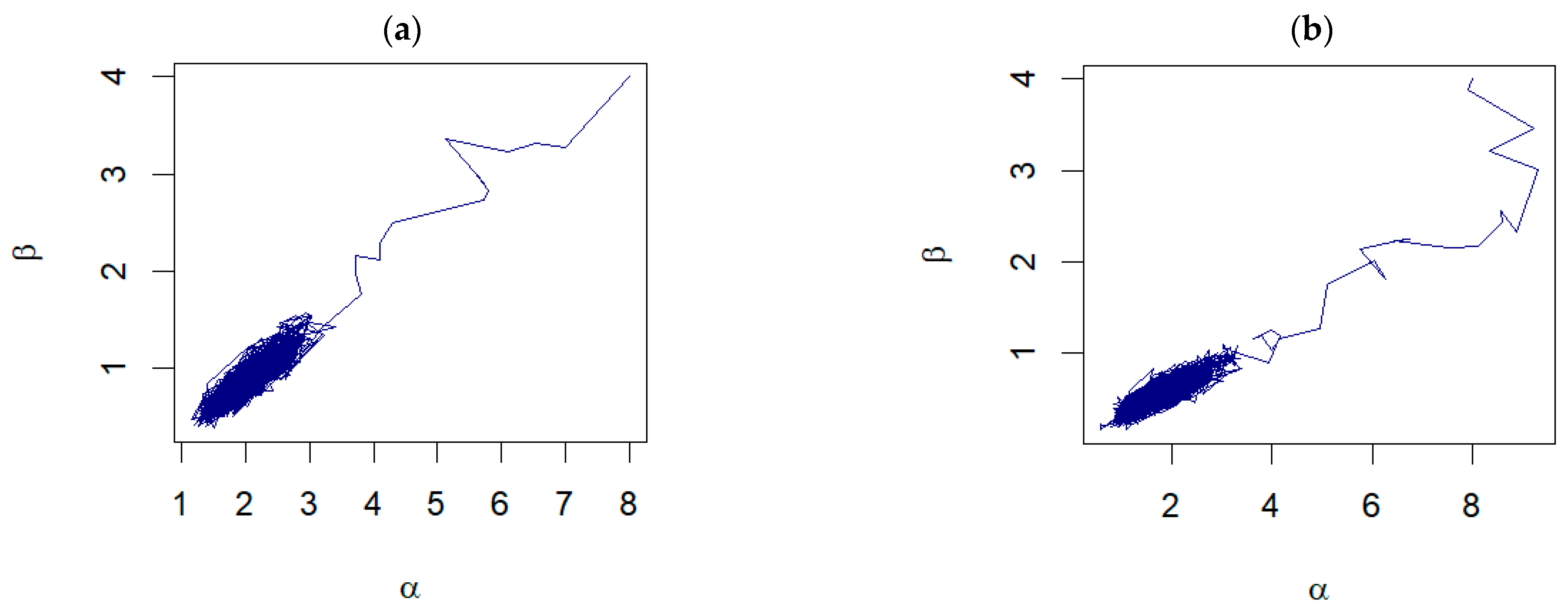
Further examination of the pair plots shown in Figure 4 reveals that, despite the initial starting points being far from the true values, the pairs of samples drawn from the RWM algorithm progress toward a densely clustered area. This dense cluster signifies the region of high probability density within the posterior distribution, illustrating the algorithm’s ability to converge to the region of interest. For unknown $\lambda$, the examples of the trace plots are shown in Figure 5.

Figure 4. The pair plots of ${\alpha }_i$ and ${\beta }_i$ from the joint posterior distributions corresponding to: (a) Prior 3 for GZTP with $\lambda =1, \alpha =2, \beta =1,$ and $n=50,$ (b) Prior 2 for CGZTP with $\lambda =0.5, \alpha =2, \beta =0.5$, and $n=25$.

Figure 5. The trace plots of ${\lambda }_i$ from posterior distributions corresponding to: (a) Prior 2 for GZTP with $\lambda =1, \alpha =1, \beta =1$, and $n=50$, (b) Prior 1 for CGZTP with $\lambda =0.5, \alpha =2, \beta =1$, and $n=50$.

Monte Carlo simulations are performed to compare the performances of the Bayes estimators with those of the classical estimators. Point estimates for parameters are averaged over 1000 iterations. Subsequently, the mean squared errors (MSEs) of the parameter estimates are calculated. The coverage probabilities (CPs) of 95% Wald confidence intervals and credible intervals and their average lengths (ALs) are determined.

Table 3 presents the detailed MLEs and MSEs obtained from simulated data sets from GZTP where the values of $\alpha$ and $\beta$ are unknown. As sample sizes increase, estimates become more accurate and the MSE values decrease. For example, for the parameter set (0.5, 2, 0.5), the MLE of α decreases from 2.3637 with an MSE of 0.8896 at sample size 15 to 2.0644 with an MSE of 0.0760 at sample size 100. It is also noticed that the MSEs of $\widehat{\alpha }$ and Bayes estimate ${\widehat{\alpha }}_B$ increase as $\alpha$ increases given that $\beta$ is fixed. For example, in a case where $\lambda =1$, β = 1, and the sample size is 15, when α is 1, the MSE for Prior 2 is 0.0566; whereas when α increases to 2, the MSE for the same prior and sample size is 0.2314. Similarly, when $\alpha$ is fixed, the MSEs of $\widehat{\beta }$ and Bayes estimate ${\widehat{\beta }}_B$ increase as $\beta$ increases. When the sample size is small, MLEs tend to have higher MSE compared to Bayesian estimates. However, between the two priors, Prior 2 has the lowest MSE. For instance, for the parameter set (0.5, 2, 0.5) and a sample size of 25, Prior 2 produces an estimate for α with an MSE of 0.1854, which is lower than the MSE of 0.2777 for Prior 1, indicating that the more informative Prior 2 generally results in a lower MSE.

Table 3. MLE and Bayesian estimates and mean squared errors of $\alpha$ and $\beta$ for the GZTP distributions.

$\left(\mathit{\lambda },\mathit{\alpha },\mathit{\beta }\right)$	$\mathit{n}$	Parameter	MLE		Prior 1		Prior 2
			Est	MSE	Est	MSE	Est	MSE
(0.5, 2, 0.5)	15	$\alpha$	2.3637	0.8896	2.1942	0.4956	2.1459	0.2622
		$\beta$	0.6240	0.0887	0.5734	0.0545	0.5550	0.0252
	25	$\alpha$	2.2284	0.4436	2.1328	0.2777	2.0948	0.1854
		$\beta$	0.5770	0.0453	0.5470	0.0282	0.5338	0.0179
	50	$\alpha$	2.1062	0.1668	2.0926	0.1516	2.0800	0.1235
		$\beta$	0.5370	0.0165	0.5299	0.0144	0.5256	0.0115
	100	$\alpha$	2.0644	0.0760	2.0508	0.0701	2.0470	0.0639
		$\beta$	0.5218	0.0072	0.5181	0.0065	0.5168	0.0059
(0.5, 2, 1)	15	$\alpha$	2.4156	1.0762	2.1780	0.4874	2.1173	0.2686
		$\beta$	1.2744	0.4485	1.1408	0.2068	1.0821	0.0921
	25	$\alpha$	2.2438	0.4768	2.153	0.2941	2.1123	0.1933
		$\beta$	1.1501	0.181	1.0977	0.1151	1.0701	0.0724
	50	$\alpha$	2.1056	0.1639	2.0762	0.1517	2.0635	0.1230
		$\beta$	1.0662	0.0646	1.0521	0.0593	1.0436	0.0472
	100	$\alpha$	2.0601	0.0846	2.0391	0.0701	2.0363	0.0638
		$\beta$	1.0404	0.0317	1.0241	0.0263	1.0221	0.0237
(1, 1, 1)	15	$\alpha$	1.1737	0.1848	1.0936	0.1119	1.0673	0.0566
		$\beta$	1.3308	0.5707	1.1928	0.2931	1.1408	0.1377
	25	$\alpha$	1.1025	0.0946	1.0639	0.0626	1.0428	0.0398
		$\beta$	1.1897	0.2654	1.1393	0.1780	1.0949	0.1005
	50	$\alpha$	1.0546	0.0410	1.0359	0.0306	1.0297	0.0246
		$\beta$	1.0831	0.0825	1.0743	0.0773	1.0613	0.0583
	100	$\alpha$	1.0222	0.0157	1.0133	0.0126	1.012	0.0114
		$\beta$	1.0335	0.0347	1.0283	0.0320	1.0255	0.0283
(1, 2, 1)	15	$\alpha$	2.4131	1.1079	2.1565	0.4129	2.1110	0.2314
		$\beta$	1.2995	0.5299	1.1395	0.1984	1.1040	0.1045
	25	$\alpha$	2.2186	0.3595	2.0983	0.2705	2.0633	0.1757
		$\beta$	1.1492	0.1642	1.0889	0.1277	1.0615	0.0782
	50	$\alpha$	2.1123	0.1617	2.0942	0.1412	2.0806	0.1149
		$\beta$	1.0762	0.0732	1.0662	0.0609	1.0562	0.0480
	100	$\alpha$	2.0594	0.0684	2.0233	0.0658	2.0207	0.0596
		$\beta$	1.0405	0.0293	1.0191	0.0277	1.0172	0.0248

Form Table 4, the 95% credible intervals and Wald confidence intervals for $\alpha$ and $\beta$ are presented. As the sample size increases, the CPs tend to approach the nominal coverage probability of 0.95, while the ALs decrease. Typically, CPs are generally above 0.95, despite the small sample size of 15. Moreover, the Prior 2 tends to have the smallest ALs with the same sample size.

Table 4. Coverage probabilities and average lengths of intervals for $\alpha$ and $\beta$ of the GZTP distributions.

$\left(\mathit{\lambda }, \mathit{\alpha }, \mathit{\beta }\right)$	$\mathit{n}$	Parameters	MLE		Prior 1		Prior 2
			CP	AL	CP	AL	CP	AL
(0.5, 2, 0.5)	15	$\alpha$	0.9730	3.0606	0.9685	2.6428	0.9846	2.3063
		$\beta$	0.9770	0.9618	0.9685	0.8251	0.9885	0.7076
	25	$\alpha$	0.9570	2.2254	0.9690	2.0294	0.9840	1.8566
		$\beta$	0.9620	0.6919	0.9640	0.6273	0.9710	0.5675
	50	$\alpha$	0.9550	1.4793	0.9500	1.4353	0.9580	1.3681
		$\beta$	0.9560	0.4570	0.9480	0.4397	0.9560	0.4172
	100	$\alpha$	0.9550	1.0235	0.9460	1.0019	0.9500	0.9777
		$\beta$	0.9570	0.3145	0.9460	0.3077	0.9550	0.3004
(0.5, 2, 1)	15	$\alpha$	0.9660	3.1336	0.9577	2.6152	0.9700	2.2779
		$\beta$	0.9660	1.9618	0.9608	1.6386	0.9831	1.3854
	25	$\alpha$	0.9610	2.2423	0.9700	2.0519	0.9810	1.8675
		$\beta$	0.9610	1.3787	0.9600	1.2565	0.9750	1.1329
	50	$\alpha$	0.9590	1.4789	0.9580	1.4253	0.9640	1.3588
		$\beta$	0.9510	0.9074	0.9480	0.8743	0.9640	0.8314
	100	$\alpha$	0.9500	1.0210	0.9420	0.9976	0.9520	0.9753
		$\beta$	0.9530	0.6271	0.9480	0.6098	0.9490	0.5949
(1, 1, 1)	15	$\alpha$	0.9770	1.3758	0.9654	1.2205	0.9831	1.0506
		$\beta$	0.9690	2.3137	0.9708	1.9558	0.9831	1.6251
	25	$\alpha$	0.9580	0.9916	0.9600	0.9296	0.9700	0.8376
		$\beta$	0.9630	1.6189	0.9550	1.4939	0.9720	1.3081
	50	$\alpha$	0.9510	0.6956	0.9420	0.6427	0.9470	0.6119
		$\beta$	0.9550	0.9973	0.9570	1.0209	0.9660	0.9580
	100	$\alpha$	0.9440	0.4748	0.9560	0.4450	0.9610	0.4338
		$\beta$	0.9450	0.6760	0.9530	0.7008	0.9620	0.6791
(1, 2, 1)	15	$\alpha$	0.9650	3.0460	0.9700	2.5165	0.9846	2.1990
		$\beta$	0.9620	2.0739	0.9715	1.6988	0.9892	1.4562
	25	$\alpha$	0.9690	2.1501	0.9630	1.9375	0.9740	1.7639
		$\beta$	0.9710	1.4321	0.9600	1.2959	0.9750	1.1647
	50	$\alpha$	0.9560	1.4393	0.9490	1.3946	0.9550	1.3289
		$\beta$	0.9580	0.9520	0.9560	0.9193	0.9640	0.8700
	100	$\alpha$	0.9580	0.9890	0.9490	0.9575	0.9520	0.9363
		$\beta$	0.9560	0.6521	0.9550	0.6301	0.9610	0.6140

Figure 6 graphically summarizes the average of estimates, MSEs, CPs, and ALs for a selected case of GZTP. In the first row, which shows estimates of α and β, there are two line graphs, one for each parameter. These results display the average estimates obtained through MLE and two Bayesian methods with different priors (Prior 1 and Prior 2). Prior 2 yields the most accuracy, followed by Prior 1 and MLE. However, as the sample size increases, the estimates from all methods converge, suggesting that larger sample sizes lead to more accurate estimations. From the second row, the bar charts show that the precision of the estimation methods improves with larger samples. Bayesian estimates, particularly those with Prior 2, tend to have lower MSEs than MLEs. In the third row, the CPs from Prior 2 tend to be higher than the others, especially in the small sample size. As the sample size increases, all the methods tend to produce about the same CP. From the last row, the ALs generally decrease as the sample size increases, showing that the intervals become narrower and, thus, more precise with larger samples. The Bayesian estimates with Prior 2 consistently show the shortest ALs across all sample sizes for both parameters.

Figure 6. The average of estimates, MSEs, CPs, and ALs for $\alpha$ and $\beta$ of the two-parameter GZTP distribution with $\lambda =0.5, \alpha =2$ and $\beta =0.5$. Column (a) presents results for the parameter α, and column (b) for the parameter β.

From simulated CGZTP datasets where the values of $\alpha$ and $\beta$ are unknown, the conclusions are consistent with those from GZTP. The detailed results are summarized in Appendix A, Table A1 and Table A2 which provide the average Bayesian estimates, MSEs, CPs, and ALs of parameters. As sample sizes increase, estimates become more accurate, and the MSE values decrease. It is observed that, while holding $\beta$ constant, the MSEs of $\widehat{\alpha }$ and ${\widehat{\alpha }}_B$ increase as $\alpha$ increases. Likewise, as $\beta$ increases, the MSEs of $\widehat{\beta }$ and Bayes estimate ${\widehat{\beta }}_B$ increase when $\alpha$ remains constant. Applying Prior 2 results in the lowest MSE values for $\alpha$ and $\beta$. Figure 7 graphically summarizes the averages of estimates, MSEs, CPs, and ALs for $\alpha$ and $\beta$ of the two-parameter CGZTP distribution with $\lambda =1, \alpha =1$, and $\beta =1$ of CGZTP.

Figure 7. The average of estimates, MSEs, CPs, and Als for $\alpha$ and $\beta$ of the two-parameter CGZTP distribution with $\lambda =1, \alpha =1, \beta =1$. Column (a) presents results for the parameter α, and column (b) for the parameter β.

For parameter λ of the GZTP distribution, the MSE values decrease as sample sizes increase, as shown in Figure 8. Both the MLE and the Jeffreys prior estimates result in poor estimations with large MSEs. As expected, the performance of these methods improves as the sample size increases. However, Prior 2 yields the lowest MSE, even with a sample size as small as 15. In all situations, the CPs either approach the desired coverage probability or exceed 0.95, and the ALs decrease as sample sizes increase. For additional scenarios, Table A3 and Table A4 in Appendix A provide a summary of all estimates, MSEs, CPs, and ALs. Similarly, the findings for λ of the CGZTP distribution are in line with those for the GZTP distribution. The MSEs of Bayesian estimates under informative priors are lower than those for the MLE and the Jeffreys prior. The CPs of credible intervals from informative priors tend to be higher than those from Wald intervals and the credible interval from the Jeffreys prior. Figure 9 presents estimates, MSEs, CPs, and ALs for three methods in a specific case, while results for other scenarios are compiled in Table A5 and Table A6.

Figure 8. The averages of estimates, MSEs, CP, and ALs for $\lambda$ of the one-parameter GZTP distribution with $\lambda =0.5, \alpha =2$, and $\beta =1$.

Figure 9. The average of estimates, MSEs, CPs, and ALs for $\lambda$ of the one-parameter CGZTP distribution with $\lambda =1, \alpha =1$, and $\beta =1$.

.

5. Application on Real Data

5.1. March Precipitation

The data in Table 5 represent the amount of precipitation (in inches) that fell in March in Minneapolis/St. Paul, including 30 consecutive measurements. These data were first discussed by Hinkley [28]. The MLE and the Bayesian summaries for $\alpha$ and $\beta$ are presented in Table 6. The MLE of the parameters are $\widehat{\alpha }=3.0597$ and $\widehat{\beta }=1.7214$ with the corresponding standard errors as 0.7207 and 0.4656, respectively. The 95% confidence intervals for $\widehat{\alpha }$ and $\widehat{\beta }$ are (1.6347, 4.4847) and (0.8086, 2.6341), respectively. Using the RWM with gamma priors and assuming λ = 0.38, the Bayesian estimates for α and β are ${\widehat{\alpha }}_B=3.0289$ and ${\widehat{\beta }}_B=1.7005$, respectively. The 95% credible intervals for $\alpha$ and $\beta$ are given, respectively, as (1.8884, 4.3697) and (0.9805, 2.6144). A histogram with the fitted GZTP curve (the orange line) and Bayesian estimates is illustrated in Figure 10. The pair plot of RWM depicted in Figure 11 illustrates that the estimates are converging to a stationary state and distributing around the posterior means, with cluster points appearing elliptical, suggesting a correlation between these two parameters. This pattern implies that Wald’s confidence intervals may not be optimal.

Table 5. March precipitation data.

0.77	1.74	0.81	1.20	1.95	1.20	0.47	1.43	3.37	2.20
3.00	3.09	1.51	2.10	0.52	1.62	1.31	0.32	0.59	0.81
2.81	1.87	1.18	1.35	4.75	2.48	0.96	1.89	0.90	2.05

Table 6. Bayesian and Maximum Likelihood Estimates with standard errors, 95% Wald CIs and Bayesian credible intervals, and goodness-of-fit testing results for two datasets.

Dataset	Method	Parameter	Estimate	Standard Error	Interval	K-S	p-Value
March precipitation	Bayes	$\alpha$	3.0289	0.6281	(1.8884, 4.3697)	0.0623	0.9998
		$\beta$	1.7055	0.4089	(0.9805, 2.6144)
	MLE	$\alpha$	3.0597	0.7270	(1.6347, 4.4847)	0.0602	0.9999
		$\beta$	1.7214	0.4656	(0.8086, 2.6341)
Remission Time	Bayes	$\alpha$	1.1697	0.1292	(0.9283, 1.4277)	0.0713	0.5341
		$\beta$	0.1246	0.0175	(0.0921, 0.1596)
	MLE	$\alpha$	1.1719	0.1312	(0.9147, 1.4290)	0.0739	0.4866
		$\beta$	0.1258	0.0174	(0.0919, 0.1599)

Figure 10. Histogram with fitted GZTP distribution for March precipitation data.

Figure 11. The pair plot of $\alpha$ and $\beta$ from the RWM algorithm for March precipitation data.

Notably, the Bayesian estimates are very close to the MLE values; however, the Bayesian credible intervals are consistently shorter than those from Wald’s confidence intervals. The Kolmogorov–Smirnov (K-S) test and the corresponding p-values indicate that both methods are effective, with Bayesian estimates exhibiting a slight performance edge over the MLEs. Note that a higher p-value indicates a better fit model.

5.2. Remission Time of Bladder Cancer Patients

The dataset consists of the number of months that 128 patients with bladder cancer spent in remission, as reported by Lee and Wang [29]. From Table 6, the MLEs of the parameters are $\widehat{\alpha }=1.1719$ and $\widehat{\beta }=0.1258$ with the corresponding 95% confidence intervals for $\widehat{\alpha }$ and $\widehat{\beta }$‚ as (0.9147, 1.4290) and (0.0919, 0.1599), respectively. Assuming that λ = 0.0238 with the unknown parameters being α and β, the Bayesian estimates for α and β are ${\widehat{\alpha }}_B=1.1697$ and ${\widehat{\beta }}_B=0.1246$, respectively. The 95% credible intervals for the parameters $\alpha$ and $\beta$ are given, respectively, by (0.9283, 1.4277) and (0.0921, 0.1596). Moreover, the K-S tests suggest that both methods can be used to model the data at a significance level of 0.05. The histogram with the fitted GZTP curve (the orange line) is illustrated in Figure 12, and the pair plot of RWM is depicted in Figure 13. Initially, there appears to be a wide spread of values indicating that the Markov chain is exploring the parameter space. As the iterations progress, the points seem to converge towards a narrower region of the plot, which suggests that the parameters are settling into a region that could represent the mode of the posterior distribution.

Figure 12. Histogram with fitted CGZTP distribution for remission time data.

Figure 13. The pair plot of $\alpha$ and $\beta$ from the RWM algorithm for remission time of bladder cancer patients.

6. Conclusions and Discussion

Both point and interval estimation have been studied within Bayesian frameworks. For point estimation, informative gamma priors with both low and high variance, as well as Jeffreys prior, are employed, and the results are compared with those obtained from MLE in terms of MSEs. Since the posterior distributions for GZTP and CGZTP do not have closed forms, the RWM algorithm is utilized to generate posterior samples. Furthermore, the Bayesian credible intervals are compared to Wald’s intervals in terms of coverage probability and average length.

Bayesian estimates using informative priors are obviously superior to the MLE and Bayesian estimates with Jeffreys priors in terms of MSEs. Among the informative priors having the mean equal to the true parameter, the one with a low variance yields a slightly lower MSE compared to that with high variance. In detail, when $\alpha$ is fixed, the MSEs of $\widehat{\beta }$ and Bayes estimate ${\widehat{\beta }}_B$ increase as $\beta$ increases. Similarly, the MSEs of $\widehat{\alpha }$ and Bayesian estimate ${\widehat{\alpha }}_B$ increase as $\alpha$ increases given that $\beta$ is fixed. In the case of an unknown λ, where the Jeffreys prior can be mathematically derived, the corresponding Bayesian estimates are slightly better than the MLE. However, as the sample size increases, the discrepancy among the MSEs obtained from all methods tends to decrease.

For interval estimation, the Bayesian credible intervals tend to be more conservative, with coverage probabilities exceeding the nominal level of 0.95, particularly for small sample sizes. The ALs of the credible intervals are notably shorter than those of the Wald confidence intervals. It is worth noting that credible intervals can achieve greater coverage with shorter interval lengths because Priors 1 and 2 were deliberately chosen so that the expected value of the prior equals the true parameter value. These informative priors have a substantial impact, often outweighing the data in their influence on the posterior. As the sample size increases, the influence of the data begins to outweigh that of the prior. In such cases, the lengths of the credible intervals tend to converge towards those of the frequentist confidence intervals, such as Wald’s intervals, and the high coverage probabilities adjust closer to the expected levels under the true confidence level.

References

- Niyomdecha, A.; Srisuradetchai, P.; Tulyanitikul, B. Gamma Zero-Truncated Poisson Distribution with the Minimum Compounded Function. Thail. Stat. Thail. 2023, 21, 863–886. [Google Scholar]
- Niyomdecha, A.; Srisuradetchai, P. Complementary Gamma Zero-Truncated Poisson Distribution and Its Application. Mathematics 2023, 11, 2584. [Google Scholar] [CrossRef]
- Xu, B.; Guo, Y.; Zhu, N. The Parameter Bayesian Estimation of Two-Parameter Exponential-Poisson Distribution and Its Optimal Property. J. Interdiscip. Math. 2016, 19, 697–707. [Google Scholar] [CrossRef]
- Yan, W.-A.; Shi, Y.-M.; Liu, Y. Bayesian Estination of Exponential Poisson Distribution under Different Loss Function. Fire Control Command Control 2012, 2, 124–126,131. [Google Scholar]
- Pathak, A.; Kumar, M.; Singh, S.K.; Singh, U. Bayesian Inference: Weibull Poisson Model for Censored Data Using the Expectation–Maximization Algorithm and Its Application to Bladder Cancer Data. J. Appl. Stat. 2022, 49, 926–948. [Google Scholar] [CrossRef] [PubMed]
- Davidson-Pilon, C. Bayesian Methods for Hackers: Probabilistic Programming and Bayesian Inference; Addison-Wesley Educational: Boston, MA, USA, 2015; pp. 127–130. [Google Scholar]
- Cai, Y.; Gui, W. Classical and Bayesian Inference for a Progressive First-Failure Censored Left-Truncated Normal Distribution. Symmetry 2021, 13, 490. [Google Scholar] [CrossRef]
- Elbatal, I.; Alotaibi, N.; Alyami, S.A.; Elgarhy, M.; El-Saeed, A.R. Bayesian and Non-Bayesian Estimation of the Nadaraj ah–Haghighi Distribution: Using Progressive Type-1 Censoring Scheme. Mathematics 2022, 10, 760. [Google Scholar] [CrossRef]
- Eliwa, M.S.; EL-Sagheer, R.M.; El-Essawy, S.H.; Almohaimeed, B.; Alshammari, F.S.; El-Morshedy, M. General Entropy with Bayes Techniques under Lindley and MCMC for Estimating the New Weibull–Pareto Parameters: Theory and Application. Symmetry 2022, 14, 2395. [Google Scholar] [CrossRef]
- Abdel-Aty, Y.; Kayid, M.; Alomani, G. Generalized Bayes Prediction Study Based on Joint Type-II Censoring. Axioms 2023, 12, 716. [Google Scholar] [CrossRef]
- Smith, A.F.M.; Roberts, G.O. Bayesian Computation via the Gibbs Sampler and Related Markov Chain Monte Carlo Methods. J. R. Stat. Soc. 1993, 55, 3–23. [Google Scholar] [CrossRef]
- Brooks, S. Markov Chain Monte Carlo Method and Its Application. J. Royal. Statistical. Soc. D 1998, 47, 69–100. [Google Scholar] [CrossRef]
- Almetwally, E.M.; Alotaibi, R.; Rezk, H. Estimation and Prediction for Alpha-Power Weibull Distribution Based on Hybrid Censoring. Symmetry 2023, 15, 1687. [Google Scholar] [CrossRef]
- Shakhatreh, M.K.; Aljarrah, M.A. Bayesian Analysis of Unit Log-Logistic Distribution Using Non-Informative Priors. Mathematics 2023, 11, 4947. [Google Scholar] [CrossRef]
- EL-Sagheer, R.M.; Almuqrin, M.A.; El-Morshedy, M.; Eliwa, M.S.; Eissa, F.H.; Abdo, D.A. Bayesian Inferential Approaches and Bootstrap for the Reliability and Hazard Rate Functions under Progressive First-Failure Censoring for Coronavirus Data from Asymmetric Model. Symmetry 2022, 14, 956. [Google Scholar] [CrossRef]
- Gelman, A.; Carlin, J.B.; Stern, H.S.; Dunson, D.B.; Vehtari, A.; Rubin, D.B. Bayesian Data Analysis, 3rd ed.; Chapman & Hall/CRC: Philadelphia, PA, USA, 2013; pp. 43–44. [Google Scholar]
- Fink, D. A Compendium of Conjugate Priors. Available online: https://courses.physics.ucsd.edu/2018/Fall/physics210b/REFERENCES/conjugate_priors.pdf (accessed on 25 December 2023).
- Naji, L.F.; Rasheed, H.A. Bayesian Estimation for Two Parameters of Gamma Distribution under Precautionary Loss Function. Ibn AL-Haitham J. Pure Appl. Sci. 2019, 32, 187–196. [Google Scholar] [CrossRef]
- Moala, F.A.; Ramos, P.L.; Achcar, J.A. Bayesian Inference for Two-Parameter Gamma Distribution Assuming Different Non-Informative Priors. Rev. Colomb. Estad. 2013, 36, 319–336. [Google Scholar]
- Pradhan, B.; Kundu, D. Bayes Estimation and Prediction of the Two-Parameter Gamma Distribution. J. Stat. Comput. Simul. 2011, 81, 1187–1198. [Google Scholar] [CrossRef]
- Anastasiou, A.; Gaunt, R.E. Wasserstein Distance Error Bounds for the Multivariate Normal Approximation of the Maximum Likelihood Estimator. Electron. J. Stat. 2021, 15, 5758–5810. [Google Scholar] [CrossRef]
- Srisuradetchai, P.; Niyomdecha, A.; Phaphan, W. Wald Intervals via Profile Likelihood for the Mean of the Inverse Gaussian Distribution. Symmetry 2024, 16, 93. [Google Scholar] [CrossRef]
- Jeffreys, H. Theory of Probability; Oxford University Press: London, UK, 1983; ISBN 9780198531937. [Google Scholar]
- Panahi, H.; Moradi, N. Estimation of the Inverted Exponentiated Rayleigh Distribution Based on Adaptive Type II Progressive Hybrid Censored Sample. J. Comput. Appl. Math. 2020, 364, 112345. [Google Scholar] [CrossRef]
- Dutta, S.; Kayal, S. Inference of a Competing Risks Model with Partially Observed Failure Causes under Improved Adaptive Type-II Progressive Censoring. Proc. Inst. Mech. Eng. O J. Risk Reliab. 2023, 237, 765–780. [Google Scholar] [CrossRef]
- Junnumtuam, S.; Niwitpong, S.-A.; Niwitpong, S. Bayesian Computation for the Parameters of a Zero-Inflated Cosine Geometric Distribution with Application to COVID-19 Pandemic Data. Comput. Model. Eng. Sci. 2023, 135, 1229–1254. [Google Scholar] [CrossRef]
- Bédard, M. On the Robustness of Optimal Scaling for Random Walk Metropolis Algorithms. Ph.D. Thesis, University of Toronto Libraries, Toronto, ON, Canada, 2006. [Google Scholar]
- Hinkley, D. On Quick Choice of Power Transformation. J. R. Stat. Soc. Ser. C Appl. Stat. 1977, 26, 67–69. [Google Scholar] [CrossRef]
- Lee, E.T.; Wang, J.W. Statistical Methods for Survival Data Analysis, 4th ed.; John Wiley & Sons: Nashville, TN, USA, 2013; ISBN 9781118095027. [Google Scholar]
Disclaimer/Publisher’s Note: The statements, opinions and data contained in all publications are solely those of the individual author(s) and contributor(s) and not of MDPI and/or the editor(s). MDPI and/or the editor(s) disclaim responsibility for any injury to people or property resulting from any ideas, methods, instructions or products referred to in the content. |
© 2024 by the authors. Licensee MDPI, Basel, Switzerland. This article is an open access article distributed under the terms and conditions of the Creative Commons Attribution (CC BY) license (https://creativecommons.org/licenses/by/4.0/).