Response Time of Queueing Mechanisms

Abstract

We study response time, a key performance characteristic of queueing mechanisms. The studied model incorporates both active and passive queue management, arbitrary service time distribution, as well as a complex model of arrivals. Therefore, the obtained formulas can be used to calculate the response time of many real queueing mechanisms with different features, by parameterizing adequately the general model considered here. The paper consists of two parts. In the first, mathematical part, we derive the distribution function for the response time, its density, and the mean value. This is done by constructing two systems of integral equations, for the distribution function and the mean value, respectively, and solving these systems with transform techniques. All the characteristics are derived both in the time-dependent and steady-state cases. In the second part, we present numerical values of the response time for a few system parameterizations and point out several of its properties, some rather counterintuitive.

1. Introduction

By the response time of a device or system, we mean the overall time a task (customer, job, networking packet, etc.) occupies the system, from entering the system until its completion. The response time of a queuing system is, by this definition, the time spent by a task in the queue while waiting for service/execution, plus the service time of this task.

The response time of most queuing systems is random in nature. Therefore, it can be fully characterized by its probability distribution or roughly by its moments (the mean, variance, etc.).

The mean response time is the principal characteristic of the performance of a queuing system (see, e.g., [1]). If we have to describe roughly the performance of a system by giving only one number, the best candidate for this number is the mean response time.

Therefore, studies on the distribution and the mean response time are of great importance. A few such studies have been carried out to date; the specifics are to be seen in the subsequent section. In short, all are devoted to queuing systems possessing some important features and mechanisms, while lacking others.

In reality, queuing systems may possess many different features and mechanisms. For instance, the arrival process may be of the Poisson type or the renewal type with arbitrary interarrival distribution. It may or may not incorporate group arrivals. The interarrival times may or may not be correlated. There may or may not be some other subtle effects present, e.g., correlation between the temporary intensity and the size of arriving groups, or correlation between sizes of groups. The service time may be of some specific type or of a general type. The queue management may be of a simple type (tail-drop) or of a more advanced type (active management).

The goal of this article is to calculate the response time in one universal queuing model, incorporating all the aforementioned possible features together. Moreover, the obtained results cover both the steady-state and time-dependent response time, as well as its distribution function, probability density, and the mean value.

Specifically, the time-dependent response time is the overall time a task arriving at a particular time t occupies the system. Therefore, it is a function of t. In practice, it is calculated for small values of t to characterize the behavior of the system shortly after its activation, when its operation is deeply influenced by its initial state. The steady-state response time characterizes the stable work of the system, i.e., for $t\to \infty$, when the influence of the initial condition vanishes.

Active queue management, built into the examined model, is the mechanism that does not permit some arriving tasks to queue up, even if the waiting room is not filled completely. In some active management mechanisms, the decision about queuing up a new task is deterministic, based on some more or less advanced calculations, see e.g., [2]. In most algorithms, however, the decision about each task is random, i.e., permission to queue up happens with some probability. This probability may change in time, being influenced by the system’s state. Furthermore, it is often assumed that this probability is dependent on the number of tasks in the system. We incorporate such a mechanism in the analyzed model. It has several important applications listed below and is, in fact, an extension of passive queue management.

By passive management (or tail drop), we mean a natural permission policy, in which a new task can queue up if and only if there is free space in the waiting room. The policy investigated here can be reduced to passive management by using the task-rejection probability represented by the Heaviside step function. In general, however, this probability can be arbitrarily related to the number of tasks in the system—tasks can be rejected long before the waiting room becomes filled completely.

Active management considered here originated in computer networking, where it was proposed to organize queues of packets in packet switching devices [3,4,5,6,7,8,9,10]. Nonetheless, the applicability of the model is much wider than that. This is because exactly the same model portrays the natural inclination of people to resign from joining a queue with a probability dependent on the queue length. The queue could be, for example, a physical queue in an amusement park [11], a virtual queue in a call center [12], a jam of cars on a motorway, and many others.

The contribution of this article is mathematical and numerical. The mathematical contribution consists of 4 new theorems devoted to the response time, presenting in particular:

• the response time distribution function in the time-dependent case (Theorem 1),
• the response time probability density in the time-dependent case (Theorem 2),
• the mean response time in the time-dependent case (Theorem 3),
• the distribution function, density and mean response time in steady state (Theorem 4).

In the numerical part, we show mean response times and densities computed for several system parameterizations, both in the time-dependent and steady-state regimes. We pay attention to how these characteristics vary with load, with the initial conditions, with the presence or lack of autocorrelation, and with task-rejection probabilities. Some unexpected behavior of the response time is noticed.

The arrival process is represented here by the batch Markovian arrival process, whose description and parameterization in the currently used form were first given in [13]. It is of utmost importance that this process can mimic many properties and nuances of real-life point processes. For example, it can imitate the interarrival distribution with arbitrary accuracy, the interarrival autocorrelation function, the group structure, the correlation between temporary arrival rate and the group size, correlation between sizes of groups, and others. Due to these qualities, it has been used in models of operation of various systems, including computer networking and telecommunications (see [14] and references therein), vehicular traffic [15,16], inventory systems [17,18], supply and maintenance systems [19,20], disaster models [21], and others.

The examined queuing model is asymmetric in the sense that the interarrival times can be autocorrelated, while the service times cannot. Such asymmetry is a trade-off between the applicability of the model and its analytical complexity. This will be debated further in Section 3.

The mathematical approach of this paper is based on constructing systems of integral equations and solving them with transform techniques. Specifically, two such systems of equations are proposed and solved: for the time-dependent distribution function of the response time (Equations (8) and (12)) and for the time-dependent mean response time (Equations (45) and (48)). The remaining characteristics of interest, i.e., densities and steady-state response times, are derived from the solutions of these two systems of equations.

The rest of the article develops as follows. In Section 2, the literature on the response time and related queuing models is reviewed. In Section 3, the modeling framework is presented, including details of the arrival process and organization of the queuing system with its active management. Several important special cases are discussed as well. Section 4 houses the paper’s key contribution, namely theorems devoted to the response time distribution function, its probability density and mean value, and steady state. In Section 5, numerical results are provided and commented on. Finally, closing remarks are given in Section 6, as well as suggestions for future work.

2. Related Work

As far as the authors know, the results of this article are new.

All the previous studies of the response time, or the related waiting time, lack one or more important features of the model examined herein, such as active management, a general type of service distribution, autocorrelated arrivals, or group arrivals. Moreover, in most papers, the analysis is reduced to the steady state only, with no time-dependent solution.

Specifically, derivations of the response time or waiting time of classic queuing models, such as M/M/1, M/G/1, and G/M/1 types, can be found in many queuing monographs, e.g., [1,22,23]. Unfortunately, these models include neither active management nor autocorrelation.

Perhaps the closest analysis is performed in [13,24], where the waiting time is computed for the model with the same arrival and service processes as herein. Specifically, the steady-state waiting time is studied in [13], while the time-dependent one in [13]. The analysis is then continued in the monograph [14], p. 161. However, the model of [13,14,24] does not incorporate a critical component examined here, i.e., active queue management. This feature significantly expands universality and applicability of the model but also requires a different analytical approach.

Conversely, there are several studies with active management in the queuing model, but without any derivations of the response time or the waiting time [25,26,27,28,29,30].

There are also other works with the same or similar model of the arrival process, but without active queue management [15,16,17,18,19,20,21,31,32,33].

Finally, there are papers that deal with the response or waiting time and do involve active queue management, but with a simplified arrival process, which either lacks group arrivals [34] or autocorrelation [35]. A general arrival process with powerful modeling capabilities is an essential feature of the model examined here.

3. Modeling Framework

We analyze the queuing model with a single service station. Namely, the arriving tasks form a queue in the waiting room in the order of arrival. Concurrently, the queue is served from the front by the service station. The service/execution time of a task is random and has a distribution function $F\left(x\right)$ of arbitrarily complex form. Service times of distinct tasks are mutually independent. The waiting room is finite and has a size of $K-1$. This means that the maximum number of tasks in the system can be K, encompassing the position for service. If upon a task arrival there are already K tasks in the system, the just-arrived task is not permitted to queue up. It exits the system unattended and never comes back.

Furthermore, any arriving task may be forbidden to queue up, even if the waiting room isn’t filled completely. This happens with a probability of $d\left(n\right)$ for each arriving task, where n denotes the number of tasks occupying the system on the arrival of this new task. This is the active management mechanism built into the model.

We see immediately that parameterizing function $d\left(n\right)$ we can obtain passive management of the system as well. Namely, if

$$\begin{array}{cc}\hfill d\left(n\right)& =\left\{\begin{array}{ccc}0,\hfill & for\hfill & n<K,\hfill \\ 1,\hfill & for\hfill & n\ge K,\hfill \end{array}\right.\hfill \end{array}$$

then a task can queue up only if the waiting room is not filled completely. This is the passive management case. If, on the other side, $d\left(n\right)\in (0,1)$ for some $n<K$, then active management takes place. In the examined model, $d\left(n\right)$ can have any form, so the derived formulas are applicable to systems with passive and active management.

The queue receives arrivals according to the batch Markovian arrival process [13]. The evolution of this process is governed by the modulating process $J\left(t\right)$, which is an m-state Markov chain with continuous time and rate matrix D. The modulating process controls arrivals of tasks, perhaps in groups.

In practice, the batch Markovian arrival process is parameterized by a sequence of $m\times m$ matrices: $D_0$, $D_1$, $D_2,\dots$. For consistency, $D_k$ must be non-negative for every $k\ge 1$, the rows of $D={\sum }_{i=0}^{\infty }{D}_i$ must sum to 0, and it must hold that $D\ne D_0$. An expanded account of characteristics and properties of this process is available in [14]. Its most important characteristic, the arrival rate, is equal to:

$$\lambda =\pi \sum _{i=1}^{\infty }i{D}_i\mathbf{1},$$

(1)

where

$$\mathbf{1}={[1,\dots ,1]}^T,$$

(2)

and $\pi$ is the steady-state vector for matrix D, fulfilling the system:

$$\pi D=[0,\dots ,0],\pi \mathbf{1}=1.$$

(3)

The mean service time is denoted by S, i.e.,:

$$S={\int }_0^{\infty }x\mathrm{d}F\left(x\right)={\int }_0^{\infty }(1-F\left(x\right))\mathrm{d}x.$$

(4)

Load of the system is therefore:

$$\rho =\lambda S,$$

(5)

where $\lambda$ is given in (1).

$N\left(t\right)$ represents the total count of tasks in the system at time t, embracing the one under service, if applicable.

Note that the considered queuing model does not possess the symmetry typical of classic queuing models, such as M/M/1 or G/G/1. In the classic models, the service and arrival processes are symmetric in the sense that all service times are uncorrelated and all interarrival times are uncorrelated. The asymmetry of the model here originates from the fact that arrival times can be highly correlated, while the service times cannot. Specifically, the k-lag correlation of the batch Markovian arrival process is as follows:

$${\rho }_c\left(k\right)=\pi D_0\mathbf{1}·\frac{\xi D_0^{-2}(D-D_0)\left({(-D_0^{-1}(D-D_0))}^{k-1}-\mathbf{1}\xi \right)D_0^{-2}(D-D_0)\mathbf{1}}{2\pi D_0^{-1}\mathbf{1}+1},$$

(6)

where $\xi$ is the steady-state vector for matrix $-D_0^{-1}(D-D_0)-I$ whereas I stands for $m\times m$ unit matrix. It is well established that ${\rho }_c\left(k\right)$ can have high values even for large k and the shape of ${\rho }_c\left(k\right)$ can be very well fitted to empirical autocorrelation functions (see, e.g., [36]).

On the other side, service times are not correlated in the examined model by definition.

Such asymmetry is a trade-off between the applicability of the model and its analytical complexity. Specifically, the arrival process is very often correlated in reality (e.g., [14,36,37]). Therefore, the applicability of symmetric models with no autocorrelation of both service and interarrival times is limited. On the other hand, correlated service times, although not impossible, are much rarer in reality than correlated arrivals. Therefore, the asymmetric model with correlated arrivals and uncorrelated services seems to constitute a reasonable choice.

Finally, by a proper parameterization of matrices $D_0$, $D_1$, $D_2,\dots$, we can obtain many simpler processes, which can also be of interest, if all the features of the full parameterization are not necessary. Specifically:

• if $m=1$ and $D_0=-\lambda$, $D_1=\lambda$, then we acquire the Poisson process,
• if $m=1$, $D_0=-\lambda$ and $j\ge 1$$D_k=p_j\lambda$, then we acquire the compound Poisson process,
• if $D_0=T$ and $D_1=-T\mathbf{1}\alpha$, then we acquire the renewal process (uncorrelated arrivals) with phase-type interarrival distribution with parameters $(\alpha ,T)$, which can approximate any renewal process with arbitrary precision,
• if $D_0=T$ and $D_k=-p_{k}T\mathbf{1}\alpha$, $k\ge 1$, then we acquire the renewal process with group arrivals,
• if $D_k=\mathbf{0}$ for $k\ge 2$, then we acquire the Markovian arrival process, which has no groups, but all the remaining features of the original process,
• if $D_0=Q-\Lambda$ and $D_1=\Lambda$, then we acquire the Markov-modulated Poisson process, the simplest autocorrelated process without group arrivals,
• if $D_j=p_j{D}_1$, $j\ge 1$, then we acquire a process with correlated interarrival times, but uncorrelated sizes of groups.

The results obtained herein are valid for arbitrary matrices $D_0$, $D_1$, $D_2,\dots$, so they can be employed in all the listed cases, and many other.

In Table 1, important model parameters and characteristics of interest are listed.

Table 1. Symbol list.

K	system capacity
$D_k$	arrival process parameters
$N\left(t\right)$	queue size at t
m	number of modulating states
$J\left(t\right)$	modulating state at t
$d\left(n\right)$	active management function
$\lambda$	arrival rate
$F\left(t\right)$	service time distribution function
S	mean service time
$\rho$	system load
${\overline{R}}_{ni}(t,x)$	distribution function of the response time at t
${\overline{r}}_{ni}(t,x)$	probability density of the response time at t
${\overline{T}}_{ni}\left(t\right)$	mean response time at t
${\overline{R}}^{\infty }\left(x\right)$	distribution function of the response time in steady state
${\overline{r}}^{\infty }\left(x\right)$	probability density of the response time in steady state
${\overline{T}}^{\infty }$	mean response time in steady state

4. Response Time

Let ${\tau }_{ni}\left(t\right)$ denote the system response time at time t, given that $N\left(0\right)=n$, $J\left(0\right)=i$. In other words, ${\tau }_{ni}\left(t\right)$ is the time it would take a task to pass the system, assuming it arrived at t and was queued up by active queue management. Note that we consider a potential, not actual arrival, at an arbitrary t.

Denote:

$${\overline{R}}_{ni}(t,x)=\mathbb{P}\{{\tau }_{ni}\left(t\right)<x|N\left(0\right)=n,J\left(0\right)=i\},t>0,x>0.$$

(7)

Therefore, ${\overline{R}}_{ni}(t,x)$ is the response time distribution function for time t, assuming initial conditions $N\left(0\right)=n$, $J\left(0\right)=i$.

As we can see, ${\overline{R}}_{ni}(t,x)$ is a time-dependent characteristic, i.e., a function of t. Computing $\overline{R}ni(t,x)$ for a small t, say $t=10$, we can characterize the response time of the system shortly after its activation, when its operation depends severely on its initial state.

We start the analysis with the case $N\left(0\right)>0$. Given this, we have:

$$\begin{array}{cc}\hfill {\overline{R}}_{ni}(t,x)=& \sum _{j=1}^m\sum _{l=0}^{K-n}{\int }_0^t{\overline{h}}_{ij}(n,l,z){\overline{R}}_{n+l-1,j}(t-z,x)\mathrm{d}F\left(z\right)\hfill \\ \hfill & +\sum _{j=1}^m\sum _{l=0}^{K-n}{\overline{h}}_{ij}(n,l,t){\int }_t^{\infty }{F}^{(n+l)\ast }(x+t-z)\mathrm{d}F\left(z\right),1\le n\le K,\hfill \end{array}$$

(8)

where $F^{\left(k\right)\ast }$ denotes the k-fold convolution of the distribution function F with itself, while ${\overline{h}}_{ij}(n,l,z)$ is probability that l tasks will be let to the waiting room by time z, and the state at time z will be j, assuming no service will be completed by z, and that it was $N\left(0\right)=n$, $J\left(0\right)=i$.

Equation (8) is created from the total probability rule applied with respect to z, the service completion moment. In the first component of (8), it is assumed $t\ge z$. Under such assumption, the new task number at z is $n+l-1$, because l new tasks are queued up by z and 1 task departs at z. Furthermore, the new modulating state at z is j. Therefore, beginning from z, the conditional probability that ${\tau }_{ni}\left(t\right)<x$ is ${\overline{R}}_{n+l-1,j}(t-z,x)$.

In the second component of (8), it is assumed $t<z$. Under such assumption, the number of tasks in the system at t is $n+l$. Therefore, we can compute directly ${\tau }_{ni}\left(t\right)$. Namely, ${\tau }_{ni}\left(t\right)$ consists of the residual time of service of the task occupying the service position at t. This residual time equals $z-t$. Then it consists of $n+l-1$ complete services of tasks present at t. Furthermore, we have to add one more service time, for the task arriving at t. In total, ${\tau }_{ni}\left(t\right)$ consists of $n+l$ complete service times, plus one partial, of duration $z-t$. This gives $\mathbb{P}\{{\tau }_{ni}\left(t\right)<x\}=F^{(n+l)\ast }(x+t-z)$.

The active management mechanism is present in Equation (8) in function ${\overline{h}}_{ij}(n,l,z)$, defined above. Naturally, ${\overline{h}}_{ij}(n,l,z)$ depends on the parameterization of the active management mechanism, through the function $d\left(n\right)$. It will be shown later how ${\overline{h}}_{ij}(n,l,z)$ can be computed and how it depends on $d\left(n\right)$ (see Formulas (61)–(67)).

The second integral in (8) can be transformed as follows:

$$\begin{array}{cc}\hfill {\int }_t^{\infty }{F}^{(n+l)\ast }(x+t-z)\mathrm{d}F\left(z\right)& ={\int }_t^{t+x}{F}^{(n+l)\ast }(x+t-z)\mathrm{d}F\left(z\right)\hfill \\ \hfill & ={\int }_0^x{F}^{(n+l)\ast }(x-z){\mathrm{d}}_{z}F(z+t).\hfill \end{array}$$

(9)

The first transformation in (9) follows from relation: $F^{(n+l)\ast }\left(t\right)=0$ for $t<0$. The second transformation is just a replacement of variables. Taking (9) into account, (8) is equivalent to:

$$\begin{array}{c}\hfill {\overline{R}}_{ni}(t,x)=\sum _{j=1}^m\sum _{l=0}^{K-n}{\int }_0^t{\overline{h}}_{ij}(n,l,z){\overline{R}}_{n+l-1,j}(t-z,x)\mathrm{d}F\left(z\right)+\sum _{j=1}^m\sum _{l=0}^{K-n}{\overline{h}}_{ij}(n,l,t)g(n+l,t,x),\end{array}$$

(10)

with

$$\begin{array}{c}\hfill g(k,t,x)={\int }_0^x{F}^{\left(k\right)\ast }(x-z){\mathrm{d}}_{z}F(z+t).\end{array}$$

(11)

Now we move to the case $N\left(0\right)=0$. Given this case, we have:

$$\begin{array}{cc}\hfill {\overline{R}}_{0i}(t,x)=& \sum _{j=1}^m\sum _{k=0}^{\infty }p(i,j,k)\sum _{l=0}^{K}q(0,k,l){\int }_0^t{\overline{R}}_{lj}(t-z,x){\mu }_i{e}^{-{\mu }_{i}z}\mathrm{d}z\hfill \\ \hfill & +F\left(x\right)e^{-{\mu }_{i}t},\hfill \end{array}$$

(12)

where $q(n,k,l)$ is probability that from k tasks arriving in a group, l taks are queued up by active queue management, assuming n taks occupied the system on this arrival of a group.

Equation (12) is created from the total probability rule applied with respect to time z, which is now an arrival or alteration of the modulating state, or both. It is known that in the batch Markovian arrival proces, group arrival of length k happens with probability $p(i,j,k)$, after a time period that has exponential distribution with mean $1/{\mu }_i$, where:

$$p(i,j,k)={\left[D_k\right]}_{i,j}/{\mu }_i,k>0.$$

(13)

$$p(i,j,0)={\left[D_0\right]}_{i,j}/{\mu }_i,i\ne j,$$

(14)

$${\mu }_i=-{\left[D_0\right]}_{i,i}.$$

(15)

In other words, $p(i,j,k)$ describes transitions of the group arrival process, i.e., the probability that the next arrival will be of size k, perhaps accompanied with an alteration of state from i to j. Specifically, if $k=0$, then merely a change of state occurs, devoid of an arrival. If $k>0$ and $i=j$, then a group arrival takes place, without a change of state. If $k>0$ and $i\ne j$, then a group arrival occurs with a change of state. Finally, simultaneous absence of arrival and absence of change of state is impossible, i.e., $p(i,i,0)=0$.

In the first component of (12), it is assumed $t\ge z$. Under such assumption, the task number at z is l, and the new modulating state at z is j. Therefore, beginning from z, the conditional probability that ${\tau }_{0i}\left(t\right)<x$ is ${\overline{R}}_{lj}(t-z,x)$. In the second component of (12) it is assumed $t<z$, which has probability $e^{-{\mu }_{i}t}$. Under assumption $t<z$, there are still 0 tasks in the system at t. Hence $\mathbb{P}\{{\tau }_{0i}\left(t\right)<x\}=F\left(x\right)$.

The active management mechanism is present in Equation (12) in function $q(0,k,l)$, defined above. It will be shown later how $q(n,k,l)$ can be derived (see Formulas (61)–(64)).

Note that (10) and (12) make up a system of $(K+1)m$ integral equations of Volterra type, for unknowns ${\overline{R}}_{ni}(t,x)$, where $0\le n\le K$ and $1\le i\le m$. We will solve this system now using the transform technique.

Denoting:

$$R_{ni}(s,x)={\int }_0^{\infty }{e}^{-st}{\overline{R}}_{ni}(t,x)\mathrm{d}t,$$

(16)

from (10) we have:

$$\begin{array}{cc}\hfill R_{ni}(s,x)=& \sum _{j=1}^m\sum _{l=0}^{K-n}{U}_{ij}(n,l,s)R_{n+l-1,j}(s,x)+\sum _{j=1}^m\sum _{l=0}^{K-n}{W}_{ij}(n,l,s,x),1\le n\le K,\hfill \end{array}$$

(17)

$$U_{ij}(n,l,s)={\int }_0^{\infty }{e}^{-st}{\overline{h}}_{ij}(n,l,z)\mathrm{d}F\left(t\right),$$

(18)

$$W_{ij}(n,l,s,x)={\int }_0^{\infty }{e}^{-st}{\overline{h}}_{ij}(n,l,t)g(n+l,t,x)\mathrm{d}t,$$

(19)

while from (12) we obtain:

$$R_{0i}(s,x)={\mu }_i{({\mu }_i+s)}^{-1}\sum _{j=1}^m\sum _{k=0}^{\infty }p(i,j,k)\sum _{l=0}^{K}q(0,k,l)R_{lj}(s,x)+F\left(x\right){({\mu }_i+s)}^{-1},$$

(20)

Then, (17) yields:

$$\begin{array}{c}\hfill R_n(s,x)=\sum _{l=0}^{K-n}U(n,l,s)R_{n+l-1}(s,x)+\sum _{l=0}^{K-n}W(n,l,s,x)\mathbf{1},1\le n\le K,\end{array}$$

(21)

where

$$R_n(s,x)={\left[R_{n1}(s,x),\dots ,R_{nm}(s,x)\right]}^T,$$

(22)

$$U(n,l,s)={\left[U_{ij}(n,l,s)\right]}_{i,j=1,\dots ,m},$$

(23)

$$W(n,l,s,x)={\left[W_{ij}(n,l,s,x)\right]}_{i,j=1,\dots ,m},$$

(24)

while (20) gives:

$$R_0(s,x)=\sum _{k=0}^{\infty }\sum _{l=0}^{K}q(0,k,l)M(k,s)R_l(s,x)+F\left(x\right)G\left(s\right),$$

(25)

with

$$M(k,s)={\left[{\mu }_i{({\mu }_i+s)}^{-1}p(i,j,k)\right]}_{i,j=1,\dots ,m},$$

(26)

$$G\left(s\right)={\left[{({\mu }_1+s)}^{-1},\dots ,{({\mu }_m+s)}^{-1}\right]}^T.$$

(27)

Lastly, denoting:

$$R(s,x)={\left[R_{01}(s,x),\dots ,R_{0m}(s,x),R_{11}(s,x),\dots ,R_{1m}(s,x),\dots ,R_{K1}(s,x),\dots ,R_{Km}(s,x)\right]}^T,$$

(28)

we can obtain the solution of (21) and (25) using standard algebraic manipulations. The result is summarized in the subsequent theorem.

Theorem 1. 

Transform of the distribution function of time-dependent response time equals:

$$R(s,x)=P^{-1}\left(s\right)Q(s,x),$$

(29)

with

$$P\left(s\right)={\left[P_{ij}\left(s\right)\right]}_{i,j=0,\dots ,K},$$

(30)

$$P_{ij}(s,x)=\left\{\begin{array}{cc}\sum _{k=0}^{\infty }q(0,k,j)M(k,s)-I,\hfill & \mathrm{if}i=j=0,\hfill \\ \\ \sum _{k=0}^{\infty }q(0,k,j)M(k,s),\hfill & \mathrm{if}i=0,j>0\hfill \\ \\ U(i,j-i+1,s)-I,\hfill & \mathrm{if}0<i<K,i=j,\hfill \\ \\ U(i,j-i+1,s),\hfill & \mathrm{if}0<i\le j+1<K+1,i\ne j,\hfill \\ \\ -I,\hfill & \mathrm{if}i=j=K,\hfill \\ \\ \mathbf{0},\hfill & \mathrm{otherwise},\hfill \end{array}\right.$$

(31)

where $\mathbf{0}$ is the $m\times m$ zero matrix and

$$Q(s,x)={\left[-F\left(x\right)G{\left(s\right)}^T,V{(1,s,x)}^T,\dots ,V{(K,s,x)}^T\right]}^T,$$

(32)

$$V(n,s,x)=-\sum _{l=0}^{K-n}W(n,l,s,x)\mathbf{1},$$

(33)

while $M(k,s)$, $G\left(s\right)$, $U(n,l,s)$ and $W(n,l,s,x)$ are defined in (26), (27), (18) and (19), respectively.

If the service distribution is absolutely continuous and has density $f\left(x\right)$, then the response time at t is also absolutely continuous and has density ${\overline{r}}_{ni}(t,x)$:

$${\overline{r}}_{ni}(t,x)\mathrm{d}x=\mathbb{P}\{{\tau }_{n,i}\left(t\right)\in \mathrm{d}x|N\left(0\right)=n,J\left(0\right)=i\},t>0,x>0.$$

(34)

Transform of this density is equal to:

$$r(s,x)=\frac{\partial R(s,x)}{\partial x},$$

(35)

where

$$r(s,x)={\left[r_{01}(s,x),\dots ,r_{0m}(s,x),r_{11}(s,x),\dots ,r_{1m}(s,x),\dots ,r_{K1}(s,x),\dots ,r_{Km}(s,x)\right]}^T,$$

(36)

$$r_{ni}(s,x)={\int }_0^{\infty }{e}^{-st}{\overline{r}}_{ni}(t,x)\mathrm{d}t.$$

(37)

To find (35), we have to calculate the derivative of $Q(s,x)$, which requires the derivative of $V(n,s,x)$, which in turn requires the derivative of $W(n,l,s,x)$, which requires the derivative of $g(k,t,x)$. In the last two steps, we need to employ the Leibniz integral rule, necessary for differentiation under integrals. By calculating all these derivatives, we get the subsequent theorem.

Theorem 2. 

If the service distribution has density $f\left(x\right)$, then the transform of density of the time-dependent response time equals:

$$r(s,x)=P^{-1}\left(s\right)z(s,x),$$

(38)

where

$$z(s,x)={\left[-f\left(x\right)G{\left(s\right)}^T,v{(1,s,x)}^T,\dots ,v{(K,s,x)}^T\right]}^T,$$

(39)

$$v(n,s,x)=-\sum _{l=0}^{K-n}w(n,l,s,x)\mathbf{1},$$

(40)

$$w(n,l,s,x)={\left[{\int }_0^{\infty }{e}^{-st}{\overline{h}}_{ij}(n,l,t)y(n+l,t,x)\mathrm{d}t\right]}_{i,j=1,\dots ,m},$$

(41)

$$\begin{array}{c}\hfill y(k,t,x)={\int }_0^x{f}^{\left(k\right)\ast }(x-z)f(z+t)\mathrm{d}z.\end{array}$$

(42)

For practical purposes, it suffices often to know the mean response time, instead of its full distribution. Let ${\overline{T}}_{ni}\left(t\right)$ denote the mean response time at t, given the initial state was $N\left(0\right)=n$, $J\left(0\right)=i$, i.e.,:

$${\overline{T}}_{ni}\left(t\right)=\mathbb{E}\left\{{\tau }_{n,i}\left(t\right)\right|N\left(0\right)=n,J\left(0\right)=i\},t>0,x>0.$$

(43)

There are at least two ways, how the mean response time can be computed. We can either use Theorem 1 with the relation:

$${\overline{T}}_{ni}\left(t\right)={\int }_0^{\infty }\left(1-{\overline{R}}_{ni}(t,x)\right)\mathrm{d}x,$$

(44)

or build equivalents of Equations (10) and (12) for ${\overline{T}}_{ni}\left(t\right)$ and solve them. In fact, the latter way is very easy, because it is straightforward to build and solve analogical equations.

Namely, for $N\left(0\right)>0$ we have:

$$\begin{array}{cc}\hfill {\overline{T}}_{ni}\left(t\right)=& \sum _{j=1}^m\sum _{l=0}^{K-n}{\int }_0^t{\overline{h}}_{ij}(n,l,z){\overline{T}}_{n+l-1,j}(t-z)\mathrm{d}F\left(z\right)\hfill \\ \hfill & +\sum _{j=1}^m\sum _{l=0}^{K-n}{\overline{h}}_{ij}(n,l,t){\int }_t^{\infty }[(n+l)S+t-z)]\mathrm{d}F\left(z\right),1\le n\le K,\hfill \end{array}$$

(45)

which is built analogously as (10). Splitting and rearranging the second integral in (45) we get:

$$\begin{array}{cc}\hfill {\overline{T}}_{ni}\left(t\right)=& \sum _{j=1}^m\sum _{l=0}^{K-n}{\int }_0^t{\overline{h}}_{ij}(n,l,z){\overline{T}}_{n+l-1,j}(t-z)\mathrm{d}F\left(z\right)\hfill \\ \hfill & +(1-F\left(t\right))S\sum _{j=1}^m\sum _{l=0}^{K-n}(n+l){\overline{h}}_{ij}(n,l,t),\hfill \\ \hfill & +a\left(t\right)\sum _{j=1}^m\sum _{l=0}^{K-n}{\overline{h}}_{ij}(n,l,t),1\le n\le K,\hfill \end{array}$$

(46)

where

$$a\left(t\right)={\int }_0^{\infty }[1-F(z+t)]\mathrm{d}z.$$

(47)

For $N\left(0\right)=0$ we have:

$$\begin{array}{c}\hfill {\overline{T}}_{0i}\left(t\right)=\sum _{j=1}^m\sum _{k=0}^{\infty }p(i,j,k)\sum _{l=0}^{K}q(0,k,l){\int }_0^t{\overline{T}}_{lj}(t-z){\mu }_i{e}^{-{\mu }_{i}z}\mathrm{d}z+S{e}^{-{\mu }_{i}t},\end{array}$$

(48)

which is built analogously as (12). Denoting:

$$T_{ni}\left(s\right)={\int }_0^{\infty }{e}^{-st}{\overline{T}}_{ni}\left(t\right)\mathrm{d}t,T_n\left(s\right)={\left[T_{n1}\left(s\right),\dots ,T_{nm}\left(s\right)\right]}^T,$$

(49)

(46) yields:

$$\begin{array}{c}\hfill T_n\left(s\right)=\sum _{l=0}^{K-n}U(n,l,s)T_{n+l-1}\left(s\right)+S\sum _{l=0}^{K-n}(n+l)Y(n,l,s)\mathbf{1}+\sum _{l=0}^{K-n}Z(n,l,s)\mathbf{1},1\le n\le K,\end{array}$$

(50)

where

$$Y(n,l,s)={\left[{\int }_0^{\infty }{e}^{-st}(1-F\left(t\right)){\overline{h}}_{ij}(n,l,t)\mathrm{d}t)\right]}_{i,j=1,\dots ,m},$$

(51)

$$Z(n,l,s)={\left[{\int }_0^{\infty }{e}^{-st}a\left(t\right){\overline{h}}_{ij}(n,l,t)\mathrm{d}t)\right]}_{i,j=1,\dots ,m}.$$

(52)

From (48) we get:

$$T_0\left(s\right)=\sum _{k=0}^{\infty }\sum _{l=0}^{K}q(0,k,l)M(k,s)T_l\left(s\right)+SG\left(s\right).$$

(53)

Using notation:

$$T\left(s\right)={\left[T_{01}\left(s\right),\dots ,T_{0m}\left(s\right),T_{11}\left(s\right),\dots ,T_{1m}\left(s\right),\dots ,T_{K1}\left(s\right),\dots ,T_{Km}\left(s\right)\right]}^T,$$

(54)

and solving the system (50) and (53), we get the subsequent theorem.

Theorem 3. 

Transform of the time-dependent mean response time equals:

$$T\left(s\right)=P^{-1}\left(s\right)H\left(s\right),$$

(55)

where

$$H\left(s\right)={\left[-SG{\left(s\right)}^T,L{(1,s)}^T,\dots ,L{(K,s)}^T\right]}^T,$$

(56)

$$L(n,s)=-S\sum _{l=0}^{K-n}(n+l)Y(n,l,s)\mathbf{1}-\sum _{l=0}^{K-n}Z(n,l,s)\mathbf{1},$$

(57)

while $P\left(s\right)$, $G\left(s\right)$, $Y(n,l,s)$ and $Z(n,l,s)$ are defined in (31), (27), (51) and (52), respectively.

Now we may obtain the response time for the system in steady state ($t\to \infty$). Let ${\overline{R}}^{\infty }\left(x\right)$ be the response time distribution function, ${\overline{r}}^{\infty }\left(x\right)$ the response time density and ${\overline{T}}^{\infty }$ the mean response time, all of them for the system in steady state.

All of these characteristics can be calculated easily from Theorems 1–3. It is done by applying the final-value theorem (see p. 89 of [38]). As the result, we get the theorem below.

Theorem 4. 

In steady state, the response time distribution function and its mean value are as follows:

$${\overline{R}}^{\infty }\left(x\right)=\underset{s\to 0+}{lim}s{R}_{01}(s,x),$$

(58)

$${\overline{T}}^{\infty }=\underset{s\to 0+}{lim}s{T}_{01}\left(s\right),$$

(59)

where $R_{01}(s,x)$ and $T_{01}\left(s\right)$ are given in Theorems 1 and 3, respectively. Moreover, if the service distribution is absolutely continuous, then the steady-state density of the response time equals:

$${\overline{r}}^{\infty }\left(x\right)=\underset{s\to 0+}{lim}s{r}_{01}(s,x),$$

(60)

where $r_{01}(s,x)$ is given in Theorem 2.

Note that the choice $N\left(0\right)=n=0$, $J\left(0\right)=i=1$ is arbitrary and does not influence the steady-state results. In fact, any other $N\left(0\right)$ and $J\left(0\right)$ can be chosen without changing the output.

Lastly, observe that to use Theorems 1–4 effectively, we must find functions $q(n,k,l)$ and ${\overline{h}}_{ij}(n,l,t)$. This can be realized using the method proposed in [28], which gives:

$$q(n,0,0)=1,q(n,k,0)=d^k\left(n\right),k>0,$$

(61)

$$q(n,0,l)=0,l>0,$$

(62)

$$q(n,k,l)=0,min\{K-n,k\}<l,$$

(63)

$$q(n,k,l)=d\left(n\right)q(n,k-1,l)+(1-d(n\left)\right)q(n+1,k-1,l-1),k>0,l>0.$$

(64)

Denoting

$$h(n,l,s)={\left[h_{ij}(n,l,s)\right]}_{i,j=1,\dots ,m},h_{ij}(n,l,s)={\int }_0^{\infty }{e}^{-st}{\overline{h}}_{ij}(n,l,t)\mathrm{d}t,$$

(65)

we obtain:

$$h(n,0,s)={(I-A(n,0,s))}^{-1}\mathrm{diag}\left(G\left(s\right)\right),$$

(66)

$$h(n,l,s)={(I-A(n,0,s))}^{-1}\sum _{j=1}^{l}A(n,j,s)h(n+j,l-j,s),l>0,$$

(67)

where

$$A(n,l,s)=\sum _{k=0}^{\infty }q(n,k,l)M(k,s).$$

(68)

5. Examples

The parameterization of task arrival process, utilized in this section, is as follows:

$$D_0=\left[\begin{array}{ccc}\hfill -0.275697& \hfill 0.262572& \hfill 0.001878\\ \hfill 0.007508& \hfill -0.181924& \hfill 0.003755\\ \hfill 0.000483& \hfill 0.000403& \hfill -0.650183\end{array}\right],$$

(69)

$$D_1=\left[\begin{array}{ccc}\hfill 0.000468& \hfill 0.001407& \hfill 0.000937\\ \hfill 0.041777& \hfill 0.000468& \hfill 0.000422\\ \hfill 0.001622& \hfill 0.000080& \hfill 0.160628\end{array}\right],$$

(70)

$$D_2=\left[\begin{array}{ccc}\hfill 0.000625& \hfill 0.001875& \hfill 0.001250\\ \hfill 0.055698& \hfill 0.000625& \hfill 0.000562\\ \hfill 0.002162& \hfill 0.000107& \hfill 0.214155\end{array}\right],$$

(71)

$$D_5=\left[\begin{array}{ccc}\hfill 0.000780& \hfill 0.002343& \hfill 0.001562\\ \hfill 0.069627& \hfill 0.000780& \hfill 0.000702\\ \hfill 0.002703& \hfill 0.000133& \hfill 0.267707\end{array}\right].$$

(72)

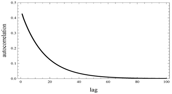
As can be noticed, the arrival process includes groups, with a maximum group size of 5. The mean group size is 3, and the arrival rate of groups is 0.333333. Thus, the overall arrival rate is 1. Moreover, this process is highly autocorrelated (see Figure 1). Its 1-lag autocorrelation is above 0.4 and remains significant up to about 100-lag.

Figure 1. Correlation of interarrival times computed for arrival process (69)–(72).

The service distribution has the following density:

$$f\left(x\right)=\frac{1}{8\rho }{e}^{-\frac{1}{2\rho }x}+\frac{9}{8\rho }{e}^{-\frac{3}{2\rho }x},x>0,\rho >0,$$

(73)

where $\rho$ is a parameter. For such density, the mean service time is:

$$S=\rho .$$

(74)

Hence, for $\lambda =1$, the parameter $\rho$ in (73) is equal to the load defined in (5). Distribution (73) has a rather moderate standard deviation, but greater than an exponential distribution would have. For example, for $\rho =1$ it equals 1.29.

If not stated differently, the following function is used for letting tasks into the waiting room:

$$\begin{array}{cc}\hfill d\left(n\right)& =\left\{\begin{array}{ccc}0,\hfill & \mathrm{for}\hfill & n<15,\hfill \\ 0.0025{(n-13)}^3,\hfill & \mathrm{for}\hfill & 15\le n<20,\hfill \\ 1,\hfill & \mathrm{for}\hfill & n\ge 20.\hfill \end{array}\right.\hfill \end{array}$$

(75)

In Table 2, we have the mean response time computed for different moments in time and for steady state. Furthermore, three different initial numbers of tasks in the system ($N\left(0\right)=0,10,20$) were assumed, with two values of load: full load, $\rho =1$, and overload, $\rho =1.5$. (Cases with $\rho <1$ are less interesting, because the response time is low there for obvious reasons).

Table 2. The mean response time, ${\overline{T}}_{n1}\left(t\right)$, for various values of load, $\rho$, and initial numbers of tasks, $N\left(0\right)$.

	$\mathit{\rho }=1,$	$\mathit{\rho }=1,$	$\mathit{\rho }=1,$	$\mathit{\rho }=1.5,$	$\mathit{\rho }=1.5,$	$\mathit{\rho }=1.5,$
	$\mathbf{N}\left(\mathbf{0}\right)=\mathbf{0}$	$\mathbf{N}\left(\mathbf{0}\right)=\mathbf{10}$	$\mathbf{N}\left(\mathbf{0}\right)=\mathbf{20}$	$\mathbf{N}\left(\mathbf{0}\right)=\mathbf{0}$	$\mathbf{N}\left(\mathbf{0}\right)=\mathbf{10}$	$\mathbf{N}\left(\mathbf{0}\right)=\mathbf{20}$
$t=1$	1.50	10.1	20.0	2.45	15.6	30.5
$t=2.5$	1.47	8.89	18.6	2.41	14.6	29.1
$t=5$	1.75	7.17	16.6	2.91	13.2	27.2
$t=10$	2.26	4.91	13.1	4.00	11.1	24.0
$t=25$	3.40	3.77	6.20	6.42	8.82	16.9
$t=50$	4.92	4.94	5.09	9.22	9.71	11.9
$t=100$	6.85	6.86	6.87	12.6	12.6	12.7
$t=250$	8.63	8.66	8.62	15.6	15.6	15.6
$t=500$	8.92	8.82	8.94	16.1	16.1	16.1
$t=\infty$	8.94	8.94	8.94	16.1	16.1	16.1

In Figure 2, Figure 3, Figure 4 and Figure 5, the response time density is depicted at different times, for 2 different values of $\rho$ and 2 values of $N\left(0\right)$. Namely, in Figure 2 and Figure 3, the fully loaded system is reflected, $\rho =1$, with $N\left(0\right)=10$ and $N\left(0\right)=20$, respectively. In Figure 4 and Figure 5, an overloaded queue is depicted, $\rho =1.5$, again with $N\left(0\right)=10$ and $N\left(0\right)=20$, respectively.

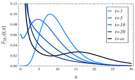
Figure 2. The response time density at different times assuming $N\left(0\right)=10$ and $\rho =1$.

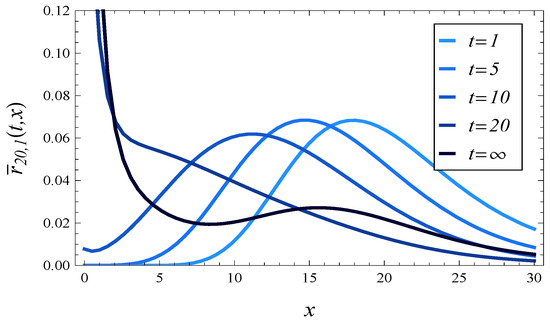
Figure 3. The response time density at different times assuming $N\left(0\right)=20$ and $\rho =1$.

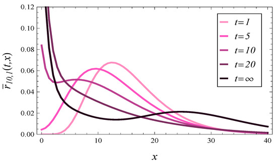
Figure 4. The response time density at different times assuming $N\left(0\right)=10$ and $\rho =1.5$.

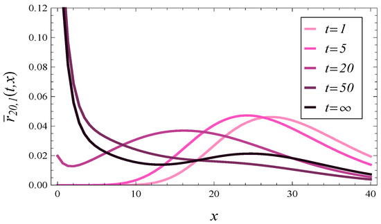
Figure 5. The response time density at different times assuming $N\left(0\right)=20$ and $\rho =1.5$.

In each of these figures, we may see the evolution of the density function towards the steady-state density (the darkest curve on each figure).

5.1. Discussion of Results

As evident in Table 2, the mean response time approaches steady state when t reaches 500. (At $t=250$, it is not stable yet, with a discrepancy of a few percent from the steady-state value.) 500 is a pretty long convergence time, most likely caused by the autocorrelation of arrivals.

We can also observe in Table 2 that the mean response time is often non-monotonic in time. Check, for instance, the case $N\left(0\right)=10$, $\rho =1$, where the response time starts at 10.1, then drops to 3.77, then grows to 8.94. Similarly in other cases.

What is surprising in Figure 2, Figure 3, Figure 4 and Figure 5 is the high concentration of probability mass near $x=0$ in steady state. It is especially unexpected in Figure 4 and Figure 5, obtained for $\rho =1.5$. One can expect that under such a high load, the queue should be long most of the time, so the response time should also be long and rarely close to zero. However, as we can see in Figure 4 and Figure 5, this is not the case.

Such behavior of the response time is to be linked with the high autocorrelation of arrivals. To demonstrate that, we can compare response times obtained for autocorrelated arrivals (69)–(72) with results for uncorrelated arrivals, parameterized simply by: $D_0=-1$, $D_1=1$.

5.2. Impact of Autocorrelation

In Figure 6 and Figure 7, the density of the response time is shown at different times in overloaded queue with $\rho =1.5$, and for $N\left(0\right)=10$ and $N\left(0\right)=20$, respectively. Both these figures were obtained for uncorrelated arrivals, $D_0=-1$, $D_1=1$.

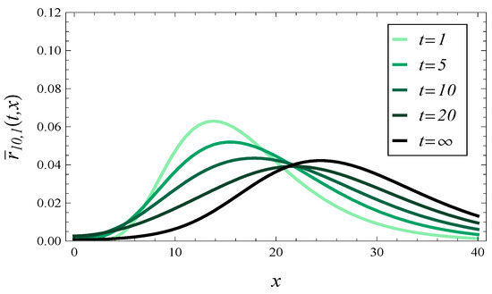
Figure 6. The response time density at different times assuming $N\left(0\right)=10$, $\rho =1.5$ and uncorrelated arrivals.

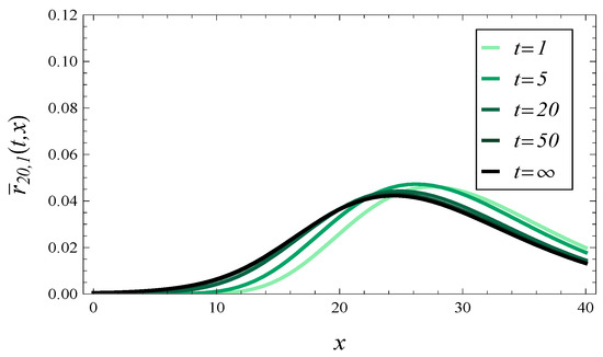
Figure 7. The response time density at different times assuming $N\left(0\right)=20$, $\rho =1.5$ and uncorrelated arrivals.

5.3. Discussion of Results

Figure 6 and Figure 7 are to be compared with Figure 4 and Figure 5, respectively.

In these pairs of figures, we may notice a very different behavior of the response time. Specifically, in Figure 4 and Figure 5, the probability mass tends to concentrate around $x=0$ as time passes. Conversely, in Figure 6 and Figure 7, the probability mass concentrates around $x=25$ as time goes on.

The effect of autocorrelation on the response time may be seen further in Figure 8. In this figure, the steady-state mean response time is shown depending on load, which varies from 0 to 2. Specifically, the blue curve reflects the mean response time for autocorrelated arrivals (69)–(72), while the green curve reflects the response time for uncorrelated ones, $D_0=-1$, $D_1=1$.

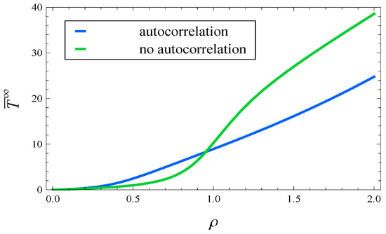
Figure 8. The mean response time in steady state versus load, for autocorrelated and uncorrelated arrivals.

As it is clear in Figure 8, for a load below 0.95, the mean response time in the autocorrelated case is greater than in the uncorrelated one. Above 0.95, however, the situation reverses – the response time is greater if there is no correlation.

This surprising effect, visible also in Figure 4, Figure 5, Figure 6 and Figure 7, can be interpreted as follows. Assume a high load, e.g., 1.5. In the correlated case, the arrival process is very irregular, i.e., it has periods of very low and very high arrival intensities. During a high-intensity phase, the queue length grows very quickly, due to the slow service. Consequently, active management kicks in aggressively, rejecting a large fraction of arriving tasks. In a low-intensity phase, a very short queue can be maintained, despite the slow service, because the arrival rate may be far less than 1 in such a phase.

In contrast, the arrival process without autocorrelation has a much more regular intensity. Therefore, the queue is moderate to long most of the time, and active management does not work so aggressively, as in the previous case.

Summarizing, when the load is high, in the autocorrelated case we have periods with short queues and periods with long queues (and extreme rejections). In the uncorrelated case, we have rather long queues most of the time (and moderate rejections). These factors make the response time shorter on average in the scenario with autocorrelated arrivals.

5.4. Impact of Active Management

In the next group of numerical results, we will investigate the effect of parameterization of active management on the response time. In all the previous examples, we used $d\left(n\right)$ given in (75). Now the following formula will be utilized:

$$d_p\left(n\right)=d(n+p),$$

(76)

i.e., (75) shifted by a parameter p. Obviously, the greater p, the more sensitive active management, and the sooner it starts rejecting tasks.

In Figure 9 and Figure 10, we can see the density of the response time in steady state for 5 values of parameter p. Figure 9 covers the case $\rho =1$, while Figure 10 covers the case $\rho =1.5$. In both figures, autocorrelated arrivals (69)–(72) are used.

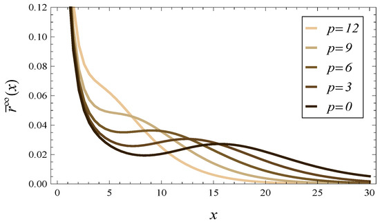
Figure 9. The steady-state response time density, for 5 values of parameter p in function $d_p\left(n\right)$ and $\rho =1$.

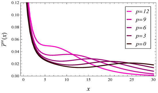
Figure 10. The steady-state response time density, for 5 values of parameters p in function $d_p\left(n\right)$ and $\rho =1.5$.

As can be noticed in Figure 9 and Figure 10, the greater p, the more probability mass is concentrated on low values of x, and the thinner the distribution tail.

5.5. Impact of Service Time Distribution

In the final set of numerical results, we will check the influence of the type of the service time distribution on the response time. So far, the hyperexponential service time (73) has been used in all numerical results. Now we will consider three more service time densities, namely:

• Pareto:

  $$f_2\left(x\right)=\frac{\alpha {\beta }^{\alpha }}{x^{\alpha +1}},x>\beta ,$$

  (77)

  with parameters $\alpha =3.236$, $\beta =0.691$,
• Weibull:

  $$f_3\left(x\right)=\frac{\alpha }{\beta }{\left(\frac{x}{\beta }\right)}^{\alpha -1}{e}^{-{(x/\beta )}^{\alpha }},x>0,$$

  (78)

  with parameters $\alpha =0.463$, $\beta =0.430$,
• gamma:

  $$f_4\left(x\right)={\beta }^{\alpha }{e}^{-\beta x}{x}^{\alpha -1}/\Gamma \left(\alpha \right),x>0,$$

  (79)

  with parameters $\alpha =0.04$, $\beta =0.04$.

All the distributions presented above have the mean value $S=1.0$. They, however, differ by the standard deviation, which is 0.5, 2.5, and 5 for densities (77)–(79), respectively.

Furthermore, we will use not only bare distributions given in (77)–(79), but also their scaled variants $\rho \xi$, where $\rho >0$ is a parameter, and $\xi$ is a random variate with one of the distributions (77)–(79). Obviously, we have $S=\rho$ in every such case, so the factor $\rho$ is equal to the load defined in (5).

5.6. Discussion of Results

In Figure 11, the mean response time in steady state is depicted for all four considered service time distributions as a function of $\rho$.

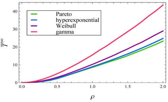
Figure 11. The mean response time in steady state versus load, for Pareto, hyperexponential, Weibull and gamma service time distribution.

We can clearly observe two things. Firstly, the general shape of the curve seems not to be affected by the particular distribution used. The shape is roughly the same for all distributions (73), (77)–(79), even though densities (73), (77)–(79) differ significantly from each other.

Secondly, the slope of each curve is deeply affected by the standard deviation of the service time. The larger the standard deviation, the steeper the curve, regardless of the particular type of distribution. For $\rho =1$, the considered standard deviations are 0.5, 1.29, 2.5 and 5, which is reflected in the same order of curves in Figure 11, from the least steep one (std. dev. of 0.5), to the most steep one (std. dev. of 5).

6. Conclusions

We studied the response time using a queuing model which incorporates both active and passive queue management, arbitrary service distribution, and a complex model of arrivals, capable of mimicking arbitrary interarrival times, group arrivals, autocorrelated arrivals, correlated group sizes, and other advanced features.

Formulas for the distribution function, probability density, and the mean value were obtained both in the time-dependent case and steady state. These formulas can be used to characterize the response time of many queuing mechanisms, possessing any subset of the aforementioned features.

In numerical examples, we observed how the response time density and its mean value are influenced by load, autocorrelation, and active queue management parameterization, both in steady state and in the time-dependent scenarios.

The most unexpected observation made was that under high load, the mean response time can be significantly smaller when arrivals are autocorrelated than when they are uncorrelated. This contradicts a simplistic view that high autocorrelation of arrivals makes all the queuing characteristics worse. In fact, autocorrelation may improve the response time, perhaps at the cost of a decline in other characteristics.

The examined model, although rather general and broadly applicable, also has some limitations. Some of these limitations are consequences of the asymmetry between the arrival and service processes in the model.

The first limitation is that arrival times can be autocorrelated, but service times cannot. In reality, arrival processes are more often correlated than service processes, but correlated services can also be encountered.

The second limitation is that the arrival process possesses a group structure, whereas the service process is singular. Again, a singular type of service is common in many systems, but examples of systems with group service can be found as well.

The third limitation is the particular active management mechanism assumed in the study. In this mechanism, a task is forbidden to queue up based on the current system occupancy. This type of active management, although popular and intuitive, is not the only one possible. The results obtained here cannot be used for other active management types.

All these limitations may directly translate into propositions for future work. Firstly, the response time of a system with autocorrelated service times can be studied. Secondly, a model allowing simultaneous service of a group of arrivals can be investigated. Finally, a model with another type of active management can be studied mathematically, e.g., of the type proposed in [39].

References

- Kleinrock, L. Queueing Systems: Theory; John Wiley and Sons: New York, NY, USA, 1975. [Google Scholar]
- Chrost, L.; Chydzinski, A. On the deterministic approach to active queue management. Telecommun. Syst. 2016, 63, 27–44. [Google Scholar] [CrossRef]
- Floyd, S.; Jacobson, V. Random early detection gateways for congestion avoidance. IEEE/Acm Trans. Netw. 1993, 1, 397–413. [Google Scholar] [CrossRef]
- Athuraliya, S.; Li, V.H.; Low, S.H.; Yin, Q. REM: Active queue management. IEEE Netw. 2001, 15, 48–53. [Google Scholar] [CrossRef]
- Zhou, K.; Yeung, K.L.; Li, V. Nonlinear RED: Asimple yet efficient active queue management scheme. Comput. Netw. 2006, 50, 3784. [Google Scholar] [CrossRef]
- Augustyn, D.R.; Domanski, A.; Domanska, J. A choice of optimal packet dropping function for active queue management. Commun. Comput. Inf. Sci. 2010, 79, 199–206. [Google Scholar]
- Domanska, J.; Augustyn, D.; Domanski, A. The choice of optimal 3-rd order polynomial packet dropping function for NLRED in the presence of self-similar traffic. Bull. Pol. Acad. Sci. Tech. Sci. 2012, 60, 779–786. [Google Scholar] [CrossRef]
- Giménez, A.; Murcia, M.A.; Amigó, J.M.; Martínez-Bonastre, O.; Valero, J. New RED-Type TCP-AQM Algorithms Based on Beta Distribution Drop Functions. Appl. Sci. 2022, 12, 11176. [Google Scholar] [CrossRef]
- Feng, C.; Huang, L.; Xu, C.; Chang, Y. Congestion Control Scheme Performance Analysis Based on Nonlinear RED. IEEE Syst. J. 2017, 11, 2247–2254. [Google Scholar] [CrossRef]
- Patel, S.; Karmeshu. A New Modified Dropping Function for Congested AQM Networks. Wirel. Pers. Commun. 2019, 104, 37–55. [Google Scholar] [CrossRef]
- Doldo, P.; Pender, J.; Rand, R. Breaking the Symmetry in Queues with Delayed Information. Int. J. Bifurc. Chaos 2021, 31, 2130027. [Google Scholar] [CrossRef]
- Rouba, I.; Mor, A.; Achal, B. Does the Past Predict the Future? The Case of Delay Announcements in Service Systems. Manag. Sci. 2016, 63, 6. [Google Scholar]
- Lucantoni, D.M. New results on the single server queue with a batch Markovian arrival process. Commun. Stat. Stoch. Model. 1991, 7, 1–46. [Google Scholar] [CrossRef]
- Dudin, A.N.; Klimenok, V.I.; Vishnevsky, V.M. The Theory of Queuing Systems with Correlated Flows; Springer: Cham, Switzerland, 2020. [Google Scholar]
- Alfa, A.S. Modelling traffic queues at a signalized intersection with vehicle-actuated control and Markovian arrival processes. Comput. Math. Appl. 1995, 30, 105. [Google Scholar] [CrossRef]
- Alfa, A.S.; Neuts, M.F. Modelling vehicular traffic using the discrete time Markovian arrival process. Transp. Sci. 1995, 29, 109–117. [Google Scholar] [CrossRef]
- Krishnamoorthy, A.; Joshua, A.N.; Kozyrev, D. Analysis of a Batch Arrival, Batch Service Queuing-Inventory System with Processing of Inventory While on Vacation. Mathematics 2021, 9, 419. [Google Scholar] [CrossRef]
- Dudin, A.; Klimenok, V. Analysis of MAP/G/1 queue with inventory as the model of the node of wireless sensor network with energy harvesting. Ann. Oper. Res. 2023, 331, 839–866. [Google Scholar] [CrossRef]
- Baek, J.W.; Lee, H.W.; Lee, S.W.; Ahn, S. A MAP-modulated fluid flow model with multiple vacations. Ann. Oper. Res. 2013, 202, 19–34. [Google Scholar] [CrossRef]
- Barron, Y. A threshold policy in a Markov-modulated production system with server vacation: The case of continuous and batch supplies. Adv. Appl. Probab. 2018, 50, 1246–1274. [Google Scholar] [CrossRef]
- Dudin, A.; Karolik, A. BMAP/SM/1 queue with Markovian input of disasters and non-instantaneous recovery. Perform. Eval. 2001, 45, 19–32. [Google Scholar] [CrossRef]
- Cohen, J.W. The Single Server Queue, Revised ed.; North-Holland Publishing Company: Amsterdam, The Netherlands, 1982. [Google Scholar]
- Takagi, H. Queueing Analysis—Finite Systems; North-Holland: Amsterdam, The Netherlands, 1993. [Google Scholar]
- Lucantoni, D.M.; Choudhury, G.L.; Whitt, W. The transient BMAP/G/1 queue. Commun. Stat. Stoch. Model. 1994, 10, 145–182. [Google Scholar] [CrossRef]
- Hao, W.; Wei, Y. An Extended GIX/M/1/N Queueing Model for Evaluating the Performance of AQM Algorithms with Aggregate Traffic. Lect. Notes Comput. Sci. 2005, 3619, 395–414. [Google Scholar]
- Kempa, W.M. Time-dependent queue-size distribution in the finite GI/M/1 model with AQM-type dropping. Acta Electrotech. Inform. 2013, 13, 85–90. [Google Scholar] [CrossRef]
- Kempa, W.M. A direct approach to transient queue-size distribution in a finite-buffer queue with AQM. Appl. Math. Inf. Sci. 2013, 7, 909–915. [Google Scholar] [CrossRef]
- Chydzinski, A.; Mrozowski, P. Queues with dropping functions and general arrival processes. PLoS ONE 2016, 11, e0150702. [Google Scholar] [CrossRef]
- Tikhonenko, O.; Kempa, W.M. Performance evaluation of an M/G/N-type queue with bounded capacity and packet dropping. Appl. Math. Comput. Sci. 2016, 26, 841–854. [Google Scholar] [CrossRef]
- Tikhonenko, O.; Kempa, W.M. Erlang service system with limited memory space under control of AQM mechanizm. Commun. Comput. Inf. Sci. 2017, 718, 366–379. [Google Scholar]
- Chydzinski, A.; Adamczyk, B. Transient and stationary losses in a finite-buffer queue with batch arrivals. Math. Probl. Eng. 2012, 2012, 326830. [Google Scholar] [CrossRef]
- Banik, A.D.; Chaudhry, M.L.; Wittevrongel, S.; Bruneel, H. A simple and efficient computing procedure of the stationary system-length distributions for GIX/D/c and BMAP/D/c queues. Comput. Oper. Res. 2022, 138, 105564. [Google Scholar] [CrossRef]
- Vishnevskii, V.M.; Dudin, A.N. Queueing systems with correlated arrival flows and their applications to modeling telecommunication networks. Autom. Remote Control 2017, 78, 1361–1403. [Google Scholar] [CrossRef]
- Chydzinski, A. Waiting Time in a General Active Queue Management Scheme. IEEE Access 2023, 11, 66535–66543. [Google Scholar] [CrossRef]
- Chydzinski, A.; Adamczyk, B. Response time of the queue with the dropping function. Appl. Math. Comput. 2020, 377, 125164. [Google Scholar] [CrossRef]
- Salvador, P.; Pacheco, A.; Valadas, R. Modeling IP traffic: Joint characterization of packet arrivals and packet sizes using BMAPs. Comput. Netw. 2004, 44, 335–352. [Google Scholar] [CrossRef]
- Lel, W.; Taqqu, M.; Willinger, W.; Wilson, D. On the self-similar nature of ethernet traffic (extended version). IEEE/ACM Trans. Netw. 1994, 2, 1–15. [Google Scholar]
- Schiff, J.L. The Laplace Transform: Theory and Applications; Springer: New York, NY, USA, 1999. [Google Scholar]
- Nichols, K.; Jacobson, V. Controlling Queue Delay. Queue 2012, 55, 42–50. [Google Scholar]
Disclaimer/Publisher’s Note: The statements, opinions and data contained in all publications are solely those of the individual author(s) and contributor(s) and not of MDPI and/or the editor(s). MDPI and/or the editor(s) disclaim responsibility for any injury to people or property resulting from any ideas, methods, instructions or products referred to in the content. |
© 2024 by the authors. Licensee MDPI, Basel, Switzerland. This article is an open access article distributed under the terms and conditions of the Creative Commons Attribution (CC BY) license (https://creativecommons.org/licenses/by/4.0/).