Statistical Inference of Normal Distribution Based on Several Divergence Measures: A Comparative Study

Abstract

Statistical predictive analysis is a very useful tool for predicting future observations. Previous literature has addressed both Bayesian and non-Bayesian predictive distributions of future statistics based on past sufficient statistics. This study focused on evaluating Bayesian and Wald predictive-density functions of a future statistic V based on a past sufficient statistic W obtained from a normal distribution. Several divergence measures were used to assess the closeness of the predictive densities to the future density. The difference between these divergence measures was investigated, using a simulation study. A comparison between the two predictive densities was examined, based on the power of a test. The application of a real data set was used to illustrate the results in this article.

1. Introduction

One of the most fundamental and significant fields in statistics is predictive analysis, which involves extracting information from historical and current data to predict future trends and behaviors. One of the many possible forms of prediction is the Bayesian predictive approach, which was first introduced by Aitchison [1], who demonstrated its advantage on the Kullback–Leibler (KL) divergence over plug-in predictive densities. Bayesian predictive-density estimation has been applied to different statistical models, including but not limited to the following: Aitchison and Dunsmore [2], who obtained Bayesian predictive distributions based on random samples from binomial, Poisson, gamma, two-parameter exponential, and normal distributions; Escobar et al. [3], who discussed the application of Bayesian inference to density-estimation models, using Dirichlet-process mixtures; and Hamura et al. [4], who used a number of Bayesian predictive densities to introduce prediction for the exponential distribution. Hamura et al. [5] studied the Bayesian prediction distribution of a chi-squared distribution, given a random sample from another chi-squared distribution under the Kullback–Leibler divergence.

Another form of prediction is the Wald predictive approach [6], which follows a non-Bayesian framework. This approach was considered via the concept of predictive likelihood [7]. Awad et al. [8] introduced a review of several prediction procedures and a comparison between them. Wald predictive density was among these procedures.

One way to check the validity of the prediction procedure is by testing the closeness between the classical distribution of future statistics and the predictive distribution by using divergence measures between the two probability distributions. Several divergence measures have been defined in the literature and have been used to measure the distance between pairs of probability-density functions.

Considering the two probability distributions $f_1\left(x\right)$ and $f_2\left(x\right)$, Kullback and Leibler [9] introduced the Kullback–Leibler divergence measure, which measures the information gain between two distributions. The Kullback–Leibler divergence measure belongs to the family of Shannon-entropy distance measures, defined as

$$K\left(f_1∥f_2\right)=E_{f_1}\left[\log \left(\frac{f_1\left(X\right)}{f_2\left(X\right)}\right)\right].$$

(1)

Lin [10] introduced the Jensen–Shannon divergence, which is a symmetric extension of the Kullback–Leibler divergence that has a finite value. In a similar approach, Johnson and Sinanovic [11] provided a new divergence measure known as the resistor-average measure. This measure is closely related to the Kullback–Leibler divergence mentioned in (1), but it is symmetric.

Do et al. [12] combined the similarity measurement of feature extraction into a joint modeling and classification scheme. They computed the Kullback–Leibler distance between the estimated models. Amin et al. [13] used the Kullback–Leibler divergence to develop a data-based Bayesian-network learning strategy; the proposed approach captures the nonlinear dependence of high-dimensional process data.

Jeffreys [14] introduced and studied a divergence measure called the Jeffreys-distance or J-divergence measure, which is considered as a symmetrization of the Kullback–Leibler divergence. The Jeffreys measure is a member of the family of Shannon-entropy distance measures, defined as

$$J(f_1,f_2)=E_{f_1}\left[\log \left(\frac{f_1\left(X\right)}{f_2\left(X\right)}\right)\right]-E_{f_2}\left[\log \left(\frac{f_1\left(X\right)}{f_2\left(X\right)}\right)\right],$$

$$J(f_1,f_2)=K\left(f_1∥f_2\right)+K\left(f_2∥f_1\right).$$

(2)

Taneja et al. [15] gave two different parametric generalizations of the Jeffreys measure. Cichocki [16] discussed the basic characteristics of the extensive families of alpha, beta, and gamma divergences including the Jeffreys divergence. They linked these divergences and showed their connections to the Tsallis and Rényi entropies. Sharma et al. [17] found the closeness between two probability distributions, using three similarity measures derived from the concepts of Jeffreys divergence and Kullback–Leibler divergence.

Rényi [18] introduced the Rényi divergence measure, which is related to Rényi entropy and depends on a parameter called r-order. The Rényi measure of order r is defined as

$$K_r^1\left(f_1∥f_2\right)=\frac{1}{r-1}\log \left(E_{f_1}\left[{\left(\frac{f_1\left(X\right)}{f_2\left(X\right)}\right)}^{r-1}\right]\right);r\ne 1,r>0.$$

(3)

Note that ${\displaystyle \underset{r\to 1}{lim}}{K}_r^1\left(f_1∥f_2\right)=K\left(f_1∥f_2\right).$ In other words, the Rényi measure of order 1 is basically the Kullback–Leibler measure.

The Rényi measure is used in physics and is called Tsallis entropy [19]. Krishnamurthy et al. [20] constructed a nonparametric estimator of Rényi divergence between continuous distributions. Their method consists of constructing estimators for certain integral functionals of two densities and transforming them into divergence estimators. Sason et al. [21] created integral formulas for the Rényi measure. Using these formulas, one can obtain bounds on the Rényi divergence as a function of the variational distance, assuming bounded relative information.

Sharma and Autar [22] suggested another generalization of Kullback–Leibler’s information, called relative information of type r, which is given by

$${ }^1{K}_r\left(f_1∥f_2\right)=\frac{1}{r-1}{E}_{f_1}\left[{\left(\frac{f_1\left(X\right)}{f_2\left(X\right)}\right)}^{r-1}-1\right];r\ne 1,r>0.$$

(4)

Note that ${\displaystyle \underset{r\to 1}{lim}}{ }^1{K}_r\left(f_1∥f_2\right)=K\left(f_1∥f_2\right).$ Taneja and Kumar [23] proposed a modified version of the relative-information-of-type-r measure as a parametric generalization of the Kullback–Leibler measure and then considered it in terms of Csiszár’s f-divergence.

Sharma and Mittal [24] generalized the Kullback–Leibler divergence measure to a measure called the r-order-and-s-degree divergence measure, defined as

$$K_r^s\left(f_1∥f_2\right)=\frac{1}{s-1}\left[{\left(E_{f_1}\left[{\left(\frac{f_1\left(X\right)}{f_2\left(X\right)}\right)}^{r-1}\right]\right)}^{\frac{s-1}{r-1}}-1\right];r,s\ne 1,r>0.$$

(5)

From Equation (5), we can see that:

(i)

${\displaystyle \underset{s\to 1}{lim}}{K}_r^s\left(f_1∥f_2\right)=K_r^1\left(f_1∥f_2\right),$ which is basically the Rényi measure defined in (3);

(ii)

${\displaystyle \underset{r\to 1}{lim}}{K}_r^s\left(f_1∥f_2\right)=K_1^s\left(f_1∥f_2\right);$ where

$$K_1^s\left(f_1∥f_2\right)=\frac{1}{s-1}\left[e^{\left((s-1)K\left(f_1∥f_2\right)\right)}-1\right];s\ne 1;$$

(iii)

${\displaystyle \underset{s\to 1}{lim}}{K}_1^s\left(f_1∥f_2\right)=K\left(f_1∥f_2\right),$ which is basically the Kullback–Leibler measure defined in (1).

Taneja and Kumar [23] conducted a full study about the r-order-and-s-degree divergence measure.

The chi-square divergence measure or Pearson ${\chi }^2$ measure [25] belongs to a family of measures called squared-$L_2$ distance measures, defined as

$${\chi }^2(f_1\parallel f_2)=E_{f_1}\left[\frac{{\left(f_1\left(X\right)-f_2\left(X\right)\right)}^2}{f_1\left(X\right)f_2\left(X\right)}\right]=E_{f_1}\left[\frac{f_1\left(X\right)}{f_2\left(X\right)}\right]-1.$$

(6)

Note that ${\chi }^2(f_1\parallel f_2)=K_2^2(f_1\parallel f_2){=}^1{K}_2(f_1\parallel f_2).$

The symmetric version of chi-square divergence is given in [23,26].

Hellinger [27] defined the Hellinger divergence measure. This measure belongs to the family of squared-chord distance measures, defined as

$$H(f_1,f_2)=\frac{1}{2}{E}_{f_1}\left[\frac{{\left(\sqrt{f_1\left(X\right)}-\sqrt{f_2\left(X\right)}\right)}^2}{f_1\left(X\right)}\right]=\frac{1}{2}{E}_{f_1}\left[{\left(1-\sqrt{\frac{f_2\left(X\right)}{f_1\left(X\right)}}\right)}^2\right].$$

(7)

Note that $H(f_1,f_2)=\frac{1}{2}{K}_{\frac{1}{2}}^{\frac{1}{2}}\left(f_1∥f_2\right)={\frac{1}{2}}^1{K}_{\frac{1}{2}}\left(f_1∥f_2\right).$

González-Castro et al. [28] estimated the prior probability that minimizes the divergence by using the Hellinger measure to measure the disparity between the test data distribution and the validation distributions generated in a fully controlled manner. Recently, Dhumras et al. [29] proposed a new kind of Hellinger measure for a single-valued neutrosophic hypersoft set and applied it to dealing with the symptomatic detection of COVID-19 data.

Bhattacharyya [30] defined the Bhattacharyya measure. This measure belongs to the family of squared-chord distance measures, defined as

$$B(f_1,f_2)=E_{f_1}\left[\sqrt{\frac{f_2\left(X\right)}{f_1\left(X\right)}}\right].$$

(8)

Note that

$$B(f_1,f_2)=1-H(f_1,f_2).$$

(9)

The Bhattacharyya measure is closely related to the Hellinger measure defined in (7).

Aherne et al. [31] presented the original geometric interpretation of the Bhattacharyya measure and explained the use of the metric in the Bhattacharyya bound. Patra et al. [32] proposed an innovative method for determining the similarity of a pair of users in sparse data. The proposed method is used to determine how the two evaluated items are relevant to each other. Similar to both Bhattacharyya’s and Hellinger’s measures, Pianka’s measure [33] between two probability distributions has values between 0 and 1. Recently, Alhihi et al. [34] introduced Pianka’s overlap coefficient for two exponential populations. A complete study of several divergence measures can be found in [26,35,36].

From the divergence measures (1)–(8), one can conclude that:

• Each of the divergence measures (1)–(6) is positive if $f_1\ne f_2$ and equals zero if and only if $f_1=f_2$.
• From (7) $0<H(f_1,f_2)<1$ if $f_1\ne f_2$ and $H(f_1,f_2)=0$ if and only if $f_1=f_2.$
• From (8), $0<B(f_1,f_2)<1$ if $f_1\ne f_2$ and $B(f_1,f_2)=1$ if and only if $f_1=f_2.$

For this paper, we evaluated the Bayesian and the Wald predictive distributions of a future statistic based on a past sufficient statistic from samples taken from the normal density. Several divergence measures were used to test the closeness between the classical distribution of the future statistic and the predictive distributions, including the two approaches: Bayesian and Wald. We used the hypothesis-testing technique to compare the behavior of these divergence measures with respect to the closure test between the two distributions. The main contribution of this work is to provide a comprehensive study of eight divergence measures in a case of normal distribution using both Bayesian and non-Bayesian (Wald) predictive approaches. To the best of our knowledge, this study has not been previously mentioned in the literature.

The rest of this paper is organized as follows: In Section 2, we evaluate the Bayesian and the Wald predictive distributions of future statistic V based on past sufficient statistic W from normal density. In Section 3, we find divergence measures between the classical distribution of future statistics and the predictive distributions found in Section 2. In Section 4, we obtain percentiles of divergence measures and test closures of the predictive distributions, using the two approaches (Bayesian and Wald) to the classical distribution. A real-life application is presented in Section 5. Finally, we provide a brief conclusion in Section 6.

2. Predictive Distributions

Let $X_1,\dots ,X_n$ be independent and identically distributed (i.i.d.) past random variables and let $Y_1,\dots ,Y_m$ be i.i.d. future random variables, where $\mathbf{X}=(X_1,\dots ,X_n)$ and $\mathbf{Y}=(Y_1,\dots ,Y_m)$ are independent. Consider a past sufficient statistic $W=r(X_1,\dots X_n)$ and a future statistic $V=u(Y_1,\dots ,Y_m)$. In this section, we construct Bayesian and Wald predictive-density functions of the future statistic V based on the past sufficient statistic W from the normal density.

2.1. Bayesian Predictive Distribution

Let $X_1,\dots ,X_n$ be $i.i.d.$ past random variables with probability-density function (pdf) $f\left(x\left|\theta \right.\right)$ and let $Y_1,\dots ,Y_m$ be $i.i.d.$ future random variables with pdf $k\left(y\left|\theta \right.\right)$. Assume that $\theta$ is a random variable with prior density $\pi \left(\theta \right)$ for $\theta \in \Theta$. Consider a past sufficient statistic $W=r(X_1,\dots ,X_n)$ with pdf $s\left(w\left|\theta \right.\right)$ and a future statistic $V=u(Y_1,\dots ,Y_m)$ with pdf $g\left(v\left|\theta \right.\right)$. The posterior-density function [37] of $\theta$, given $W=w$, is defined as

$$p\left(\theta \left|w\right.\right)=\frac{s\left(w\left|\theta \right.\right)\pi \left(\theta \right)}{\underset{\Theta }{\int }s\left(w\left|\theta \right.\right)\pi \left(\theta \right)d\theta }.$$

(10)

The following theorem provides a Bayesian method to construct predictive distributions.

Theorem 1 

([37]). Let $W=r(X_1,\dots ,X_n)$ be a past sufficient statistic and let θ be a random variable with prior density $\pi \left(\theta \right)$ for $\theta \in \Theta .$ Assume that $V=u(Y_1,\dots ,Y_m)$ is a future statistic with pdf $g(v\left|\theta \right)$. The Bayesian predictive-density function of V, given $W=w$, is given by

$$h\left(v\left|w\right.\right)=\underset{\Theta }{\int }g\left(v\left|\theta \right.\right)p\left(\theta \left|w\right.\right)d\theta ,$$

(11)

 where $p\left(\theta \left|w\right.\right)$ is the posterior-density function of θ, given $W=w$, defined in (10).

The next two theorems provide the Bayesian predictive distributions for some statistics. Theorem 2 below presents the Bayesian predictive distribution of the future statistic $V={\sum }_{i=1}^m{Y}_i$ based on the past sufficient statistic $W={\sum }_{i=1}^n{X}_i$ from random samples taken from normal density; the choice of these statistics is based on the fact that we need statistics that best describe the characteristics of the data set, and they are closely related to the mean of the data set. Note that the choice of W is a completely sufficient statistic for the parameter under consideration. A similar result is obtained in Theorem 4 for the same statistics V and W, to obtain the Wald predictive distribution.

We use the following notations to represent some distributions that appear in the results of Theorems 2 and 3 below: the normal distribution with mean $\mu$ and variance ${\sigma }^2$ is denoted by $N(\mu ,{\sigma }^2)$; the gamma distribution with shape parameter $\alpha$ and scale parameter $\beta$ is denoted by Gamma$(\alpha ,\beta );$ and the generalized inverted beta distribution with shape parameters $\alpha ,\beta$, and p is denoted by InBe$(\alpha ,\beta ,p)$.

Theorem 2. 

Let $X_1,\dots ,X_n\stackrel{i.i.d.}{\sim }$ $N({\theta }_1,1/{\theta }_2)$and $Y_1,\dots ,Y_m\stackrel{i.i.d.}{\sim }$ $N(\delta {\theta }_1,1/{\theta }_2)$, where δ is known. Assume that $\mathbf{X}=(X_1,\dots ,X_n)$ and $\mathbf{Y}=(Y_1,\dots ,Y_m)$ are independent and that $V={\sum }_{i=1}^m{Y}_i$ and $W={\sum }_{i=1}^n{X}_i.$ If ${\theta }_2$ is known and ${\theta }_1$ is unknown with prior distribution $N(a,1/b)$, where a and b are assumed to be known, the Bayesian predictive distribution of V, given $W=w$, is

$$N\left(\frac{m\delta (ab+w{\theta }_2)}{b+n{\theta }_2},\frac{m\left(b+(n+m{\delta }^2){\theta }_2\right)}{(b+n{\theta }_2){\theta }_2}\right).$$

(12)

Proof. 

It is easy to see that the past sufficient statistic $W={\sum }_{i=1}^n{X}_i$, given ${\theta }_1,$ follows the normal distribution $N(n{\theta }_1,n/{\theta }_2)$ and that $V={\sum }_{i=1}^m{Y}_i$, given ${\theta }_1$, follows the normal distribution $N(m\delta {\theta }_1,m/{\theta }_2)$. In other words, the classical distribution of the future statistic V, given ${\theta }_1$, is

$$g\left(v\left|{\theta }_1\right.\right)=\sqrt{\frac{{\theta }_2}{2\pi m}}exp\left\{-\frac{{\theta }_2}{2m}{\left(v-m\delta {\theta }_1\right)}^2\right\}.$$

(13)

Now, using (10), the posterior-density function of ${\theta }_1$, given $W=w$, is equal to

$$\begin{array}{cc}\hfill p\left({\theta }_1\right|w)& \propto exp\left\{-\frac{{\theta }_2}{2n}{(w-n{\theta }_1)}^2\right\}exp\left\{-\frac{b}{2}{({\theta }_1-a)}^2\right\}\hfill \\ \hfill & \propto exp\left\{-\left(\frac{b+n{\theta }_2}{2}\right){\left({\theta }_1-\frac{ab+w{\theta }_2}{b+n{\theta }_2}\right)}^2\right\}.\hfill \end{array}$$

Therefore, the posterior-density function of ${\theta }_1,$ given $W=w$, is the normal distribution $N\left(\frac{ab+w{\theta }_2}{b+n{\theta }_2},\frac{1}{b+n{\theta }_2}\right)$.

Applying Equation (11), the Bayesian predictive-density function of V, given $W=w$, can be derived as

${\displaystyle h\left(v\left|w\right.\right)={\int }_{-\infty }^{\infty }\sqrt{\frac{{\theta }_2}{2\pi m}}\exp \left\{-\frac{{\theta }_2}{2m}{\left(v-m\delta {\theta }_1\right)}^2\right\}·\sqrt{\frac{b+n{\theta }_2}{2\pi }}\exp \left\{-\left(\frac{b+n{\theta }_2}{2}\right){\left({\theta }_1-\frac{ab+w{\theta }_2}{b+n{\theta }_2}\right)}^2\right\}d{\theta }_1.}$

By evaluating this integral, the Bayesian predictive-density function of V, given $W=w$, is

$$h\left(v\left|w\right.\right)=\sqrt{\frac{(b+n{\theta }_2){\theta }_2}{2\pi m(b+(n+m{\delta }^2){\theta }_2)}}exp\left\{-\frac{(b+n{\theta }_2){\theta }_2}{2m\left(b+(n+m{\delta }^2){\theta }_2\right)}{\left(v-\frac{\delta m(ab+w{\theta }_2)}{b+n{\theta }_2}\right)}^2\right\},$$

(14)

where $-\infty <v<\infty ,-\infty <w<\infty .$

Which represents the normal distribution $N\left(\frac{m\delta (ab+w{\theta }_2)}{b+n{\theta }_2},\frac{m\left(b+(n+m{\delta }^2){\theta }_2\right)}{(b+n{\theta }_2){\theta }_2}\right)$. □

The following theorem presents the Bayesian predictive distribution of the future statistic $V={\sum }_{i=1}^m{(Y_i-{\theta }_1)}^2$ based on the past sufficient statistic $W={\sum }_{i=1}^n{(X_i-{\theta }_1)}^2$ from random samples taken from normal density. The choice of these statistics is based on the fact that we need statistics that best describe the characteristics of the data set. The choice of V and W is closely related to the variance of the data set, and it is often used to represent data too. Note that a similar result is obtained in Theorem 5 for the same statistics V and W, to obtain the Wald predictive distribution.

Theorem 3. 

Let $X_1,\dots ,X_n\stackrel{iid}{\sim }$ $N({\theta }_1,1/{\theta }_2)$and $Y_1,\dots ,Y_m\stackrel{iid}{\sim }$ $N({\theta }_1,\delta /{\theta }_2),$ where δ is known. Assume that $\mathbf{X}=(X_1,\dots ,X_n)$ and $\mathbf{Y}=(Y_1,\dots ,Y_m)$ are independent and that $V={\sum }_{i=1}^m{(Y_i-{\theta }_1)}^2$ and $W={\sum }_{i=1}^n{(X_i-{\theta }_1)}^2.$ If ${\theta }_1$ is known and ${\theta }_2$ is unknown with prior distribution Gamma$(a,1/b)$, where a and b are assumed to be known, the Bayesian predictive distribution of V, given $W=w$, is

$$InBe(\frac{m}{2},\frac{n}{2}+a,\delta (w+2b)).$$

(15)

Proof. 

It is easy to see that the past sufficient statistic $W={\sum }_{i=1}^n{(X_i-{\theta }_1)}^2$, given ${\theta }_2$, follows the gamma distribution Gamma$\left(\frac{n}{2},\frac{2}{{\theta }_2}\right)$ and that $V={\sum }_{i=1}^m{(Y_i-{\theta }_1)}^2$, given ${\theta }_2$, follows Gamma$\left(\frac{m}{2},\frac{2\delta }{{\theta }_2}\right).$ Using Equation (10), the posterior-density function of ${\theta }_2$, given $W=w$, is Gamma$\left(\frac{n+2a}{2},\frac{2}{w+2b}\right)$. Applying Equation (11), the Bayesian predictive-density function of V, given $W=w$, can be derived as

$$\begin{array}{cc}\hfill h\left(v\left|w\right.\right)& ={\int }_0^{\infty }\frac{v^{(m/2-1)}{\left(\frac{{\theta }_2}{2\delta }\right)}^{(m/2)}exp\left\{-\frac{{\theta }_2}{2\delta }v\right\}}{\Gamma \left(\frac{m}{2}\right)}·\frac{{\theta }_2^{\left((n+2a)/2\right)-1}{\left(\frac{w+2b}{2}\right)}^{(n+2a)/2}exp\left\{-{\theta }_2\left(\frac{w+2b}{2}\right)\right\}}{\Gamma \left(\frac{n+2a}{2}\right)}d{\theta }_2\hfill \\ \hfill & =\frac{v^{\left(m/2-1\right)}{\left(\delta (w+2b)\right)}^{(n+2a)/2}}{B(\frac{m}{2},\frac{n+2a}{2}){(v+\delta (w+2b))}^{(m+n+2a)/2}},\mathrm{where}v>0\mathrm{and}w>0.\hfill \end{array}$$

As a result, the Bayesian predictive-density function of V, given $W=w$, follows the generalized inverted beta distribution InBe$\left(\frac{m}{2},\frac{n+2a}{2},\delta (w+2b)\right)$. □

2.2. Wald Predictive Distribution

In this subsection, the Wald predictive-density function of the future statistic V based on the past sufficient statistic W from normal density is derived.

Let $X_1,\dots ,X_n$ be $i.i.d.$ past random variables with pdf $f(x;\theta )$ and let $Y_1,\dots ,Y_m$ be $i.i.d.$ future random variables with pdf $k(y;\theta )$, where {$\theta \in \Theta$} is an unknown parameter and $\mathbf{X}=(X_1,\dots ,X_n)$ and $\mathbf{Y}=(Y_1,\dots ,Y_m)$ are independent. Consider a past sufficient statistic $W=r(X_1,\dots ,X_n)$ with pdf $s(w;\theta )$ and future statistic $V=u(Y_1,\dots ,Y_m)$ with pdf $g(v;\theta )$. The Wald predictive-density function [6] of V, given $W=w$, is defined as

$$q\left(v\left|w\right.\right)=g(v;{\widehat{\theta }}_w),$$

(16)

where ${\widehat{\theta }}_W$ is the maximum likelihood estimator (MLE) of $\theta$ based on the distribution of the past sufficient statistic W, for which

$$\underset{\theta }{sup}L\left(\theta \right)=L\left({\widehat{\theta }}_W\right),\mathrm{where}L\left(\theta \right)=s(w;\theta ).$$

The next two theorems present the Wald predictive distribution for some statistics. Theorem 4 considers the future statistic $V={\sum }_{i=1}^m{Y}_i$ and the past sufficient statistic $W={\sum }_{i=1}^n{X}_i,$ while Theorem 5 considers the future statistic $V={\sum }_{i=1}^m{(Y_i-{\theta }_1)}^2$ and the past sufficient statistic $W={\sum }_{i=1}^n{(X_i-{\theta }_1)}^2.$

Theorem 4. 

Let $X_1,\dots ,X_n\stackrel{iid}{\sim }$ $N({\theta }_1,1/{\theta }_2)$and $Y_1,\dots ,Y_m\stackrel{iid}{\sim }$ $N(\delta {\theta }_1,1/{\theta }_2)$, where δ is known. Assume that $\mathbf{X}=(X_1,\dots ,X_n)$ and $\mathbf{Y}=(Y_1,\dots ,Y_m)$ are independent and that $V={\sum }_{i=1}^m{Y}_i$ and $W={\sum }_{i=1}^n{X}_i.$ If ${\theta }_1$ is unknown and${\theta }_2$ is known, the Wald predictive distribution of V, given $W=w$, is

$$N\left(\frac{\delta mw}{n},\frac{m}{{\theta }_2}\right).$$

(17)

Proof. 

Using the fact that $W={\displaystyle \sum _{i=1}^n}{X}_i$ follows $N\left(n{\theta }_1,\frac{n}{{\theta }_2}\right)$, we obtain

$$L\left({\theta }_1\right)=s(w;{\theta }_1)=\sqrt{\frac{{\theta }_2}{2n\pi }}exp\left\{-\frac{{\theta }_2}{2n}{(w-n{\theta }_1)}^2\right\};-\infty <{\theta }_1<\infty ,-\infty <w<\infty .$$

As a result, the MLE of ${\theta }_1$ is ${\widehat{{\theta }_1}}_W=\frac{W}{n}.$ Now, the distribution of $V={\displaystyle \sum _{i=1}^m}{Y}_i$ is $N\left(m\delta {\theta }_1,\frac{m}{{\theta }_2}\right)$. By applying Equation (16), the Wald predictive distribution of V, given $W=w$, is equal to

$$q\left(v\left|w\right.\right)=\sqrt{\frac{{\theta }_2}{2m\pi }}exp\left\{-\frac{{\theta }_2}{2m}{\left(v-\frac{\delta mw}{n}\right)}^2\right\};v>0,w>0,$$

(18)

which represents the normal distribution $N\left(\frac{\delta mw}{n},\frac{m}{{\theta }_2}\right)$ as required. □

Theorem 5. 

Let $X_1,\dots ,X_n\stackrel{iid}{\sim }$ $N({\theta }_1,1/{\theta }_2)$and $Y_1,\dots ,Y_m\stackrel{iid}{\sim }$ $N({\theta }_1,\delta /{\theta }_2),$ where δ is known. Assume that $\mathbf{X}=(X_1,\dots ,X_n)$ and $\mathbf{Y}=(Y_1,\dots ,Y_m)$ are independent and that $V={\sum }_{i=1}^m{(Y_i-{\theta }_1)}^2$ and $W={\sum }_{i=1}^n{(X_i-{\theta }_1)}^2.$ If ${\theta }_1$ is known and ${\theta }_2$ is unknown, the Wald predictive distribution of V, given $W=w$, is

$$Gamma\left(\frac{m}{2},\frac{2\delta w}{n}\right).$$

(19)

Proof. 

Using the fact that the past sufficient statistic $W={\sum }_{i=1}^n{(X_i-{\theta }_1)}^2$ follows Gamma$\left(\frac{n}{2},\frac{2}{{\theta }_2}\right)$, we obtain

$$L\left({\theta }_2\right)=s(w;{\theta }_2)=\frac{w^{\frac{n}{2}-1}{\left(\frac{{\theta }_2}{2}\right)}^{\frac{n}{2}}{e}^{-\frac{{\theta }_2}{2}w}}{\Gamma \left(\frac{n}{2}\right)};{\theta }_2>0,w>0.$$

As a result, the MLE of ${\theta }_2$ is ${\widehat{{\theta }_2}}_W=\frac{n}{W}.$ Now, the distribution of $V={\sum }_{i=1}^m{(Y_i-{\theta }_1)}^2$ follows Gamma$\left(\frac{m}{2},\frac{2\delta }{{\theta }_2}\right)$. By applying (16), we obtain the result that the Wald predictive distribution of V, given $W=w$, follows Gamma$\left(\frac{m}{2},\frac{2\delta w}{n}\right)$ as required. □

3. Divergence Measures between the Classical Distribution of Future Statistic and Predictive Distributions

In this section, several divergence measures between the classical distribution of the future statistic V and the predictive distribution of V, given the past sufficient statistic W, are found for both prediction cases—Bayesian and Wald—by considering the future statistic $V={\sum }_{i=1}^m{Y}_i$ and the past sufficient statistic $W={\sum }_{i=1}^n{X}_i$, where the Bayesian and Wald predictive distributions are found in Theorems 2 and 4, respectively. The other case, where $V={\sum }_{i=1}^m{(Y_i-{\theta }_1)}^2$ and $W={\sum }_{i=1}^n{(X_i-{\theta }_1)}^2$ can be considered as a possible idea for future research.

The next theorem gives formulas for the following divergence measures between the classical distribution of the future statistic $g\left(v\left|{\theta }_1\right.\right)$ in Equation (13) and the Bayesian predictive distribution $h\left(v\left|w\right.\right)$ in Equation (14): the Kullback–Leibler measure ($K(g\parallel h)$), the Jeffreys measure ($J(g,h)$), the Rényi measure ($K_r^1(g\parallel h)$), the relative-information-of-type-r measure (${ }^1{K}_r(g\parallel h)$), the r-order-and-s-degree measure ($K_r^s(g\parallel h)$), the chi-square measure (${\chi }^2(g\parallel h)$), the Hellinger measure ($H(g,h)$), and the Bhattacharyya measure ($B(g,h)$).

For each of the aforementioned measures, we also find its average under the prior distribution of ${\theta }_1$. For instance, the Kullback–Leibler measure and its average under the prior distribution of $\theta$ between the two densities g and h, respectively, are presented as

$$K\left(g∥h\right)=E_g\left[\log \left(\frac{g\left(V\left|{\theta }_1\right.\right)}{h\left(V\left|w\right.\right)}\right)\right]\mathrm{and}AK\left(g∥h\right)=E_{{\theta }_1}{E}_g\left[\log \left(\frac{g\left(V\left|{\theta }_1\right.\right)}{h\left(V\left|w\right.\right)}\right)\right].$$

Similarly, the average of the divergence measures under the prior distribution of ${\theta }_1$ between two probability density functions g and h for each of the remaining divergence measures are denoted as $AK\left(g∥h\right),$ $AJ(g,h),$ $A{K}_r^1\left(g∥h\right),$ $A^1{K}_r\left(g∥h\right),$ $A{K}_r^s\left(g∥h\right),$ $A{K}_1^s\left(g∥h\right),$ $A{\chi }^2\left(g∥h\right),$ and $AH(g,h).$

Theorem 6. 

Under the assumption of Theorem 2, let $g\left(v\right|{\theta }_1)$ be the classical distribution of the future statistic and let $h\left(v\right|w)$ be the Bayesian predictive distribution of V, given $W=w$, from the normal density. The value of the following divergence measures and their average under the prior distribution of ${\theta }_1$ between $g\left(v\right|{\theta }_1)$ and $h\left(v\right|w)$—(1) the Kullback–Leibler measure, (2) the Jeffreys measure, (3) the Rényi measure, (4) the relative-information-of-type-r measure, (5) the r-order-and-s-degree measure, (6) the chi-square measure, (7) the Hellinger measure, and (8) the Bhattacharyya measure—are equal to, respectively:

(1) 

$K(g\parallel h)=\frac{1}{2}\log \left(\frac{b+(n+m{\delta }^2){\theta }_2}{b+n{\theta }_2}\right)+\frac{m{\delta }^2(b+n{\theta }_2){\theta }_2}{2(b+(n+m{\delta }^2){\theta }_2)}\left({\left({\theta }_1-\frac{ab+w{\theta }_2}{b+n{\theta }_2}\right)}^2-\frac{1}{b+n{\theta }_2}\right),$ and

$AK\left(g∥h\right)=\frac{1}{2}\log \left(\frac{b+(n+m{\delta }^2){\theta }_2}{b+n{\theta }_2}\right)+\frac{m{\delta }^2(b+n{\theta }_2){\theta }_2}{2(b+(n+m{\delta }^2){\theta }_2)}\left({\left(a-\frac{ab+w{\theta }_2}{b+n{\theta }_2}\right)}^2+\frac{n{\theta }_2}{b+n{\theta }_2}\right);$

(2) 

$J(g,h)=\frac{m{\delta }^2{\theta }_2}{2(b+(n+m{\delta }^2){\theta }_2)}\left(\frac{m{\delta }^2{\theta }_2}{b+n{\theta }_2}+\left(m{\delta }^2{\theta }_2+2(b+n{\theta }_2)\right){({\theta }_1-\frac{ab+w{\theta }_2}{b+n{\theta }_2})}^2\right),$ and

$AJ(g,h)=\frac{m{\delta }^2{\theta }_2}{2(b+(n+m{\delta }^2){\theta }_2)}\left(\frac{m{\delta }^2{\theta }_2}{b+n{\theta }_2}+\left(m{\delta }^2{\theta }_2+2(b+n{\theta }_2)\right)\left({(a-\frac{ab+w{\theta }_2}{b+n{\theta }_2})}^2+\frac{1}{b}\right)\right);$

(3) 

$K_r^1\left(g∥h\right)=\frac{1}{2(r-1)}\log \left(\frac{b+(n+m{\delta }^2){\theta }_2}{b+(n+mr{\delta }^2){\theta }_2}\right)+\frac{1}{2}\log \left(\frac{b+(n+m{\delta }^2){\theta }_2}{b+n{\theta }_2}\right)+\frac{mr(b+n{\theta }_2){\delta }^2{\theta }_2}{2(b+(n+mr{\delta }^2){\theta }_2)}{\left({\theta }_1-\frac{ab+w{\theta }_2}{b+n{\theta }_2}\right)}^2,$ where $r\ne 1,r>0,$ and

$A{K}_r^1\left(g∥h\right)=\frac{1}{2(r-1)}\log \left(\frac{b(b+(n+mr{\delta }^2){\theta }_2)}{c}\right)+\frac{bmr{(w-an)}^2{\delta }^2{\theta }_2^3}{2(b+n{\theta }_2)c},$ where $r\ne 1,r>0,c>0;$

(4) 

${ }^1{K}_r\left(g∥h\right)=\frac{1}{r-1}\left(-1+{\left(\frac{b+(n+m{\delta }^2){\theta }_2}{b+n{\theta }_2}\right)}^{\frac{r-1}{2}}\sqrt{\frac{b+(n+m{\delta }^2){\theta }_2}{b+(n+mr{\delta }^2){\theta }_2}}\right.\times \left.exp\left\{\frac{mr(r-1)(b+n{\theta }_2){\delta }^2{\theta }_2}{2(b+(n+mr{\delta }^2){\theta }_2)}{\left({\theta }_1-\frac{ab+w{\theta }_2}{b+n{\theta }_2}\right)}^2\right\}\right),$ where $r\ne 1,r>0,$ and

$A^1{K}_r\left(g∥h\right)=\frac{1}{r-1}\left(-1+\sqrt{\frac{b(b+(n+mr{\delta }^2){\theta }_2)}{c}}exp\left\{\frac{bmr(r-1){(w-an)}^2{\delta }^2{\theta }_2^3}{2(b+n{\theta }_2)c}\right\}\right),$ where $r\ne 1,r>0,c>0;$

(5) 

$K_r^s(g\left.∥h\right)=\frac{1}{s-1}\left(-1+{\left(\frac{b+(n+m{\delta }^2){\theta }_2}{b+n{\theta }_2}\right)}^{\frac{s-1}{2}}{\left(\frac{b+(n+m{\delta }^2){\theta }_2}{b+(n+mr{\delta }^2){\theta }_2}\right)}^{\frac{s-1}{2(r-1)}}\right.\times \left.exp\left\{\frac{mr(s-1)(b+n{\theta }_2){\delta }^2{\theta }_2}{2(b+(n+mr{\delta }^2){\theta }_2)}{\left({\theta }_1-\frac{ab+w{\theta }_2}{b+n{\theta }_2}\right)}^2\right\}\right),$ where $r,s\ne 1,r>0,$ and

$A{K}_r^s\left(g∥h\right)=\frac{1}{s-1}\left(-1+{\left(\frac{b(b+(n+mr{\delta }^2){\theta }_2)}{c}\right)}^{\frac{s-1}{2(r-1)}}exp\left\{\frac{bmr(s-1){(w-an)}^2{\delta }^2{\theta }_2^3}{2(b+n{\theta }_2)c}\right\}\right),$ where $r,s\ne 1,r>0,c>0;$

(6) 

${\chi }^2\left(g∥h\right)=-1+\sqrt{\frac{b+(n+m{\delta }^2){\theta }_2}{b+n{\theta }_2}}\sqrt{\frac{b+(n+m{\delta }^2){\theta }_2}{b+(n+2m{\delta }^2){\theta }_2}}exp\left\{\frac{mr(b+n{\theta }_2){\delta }^2{\theta }_2}{2(b+(n+mr{\delta }^2){\theta }_2)}{\left({\theta }_1-\frac{ab+w{\theta }_2}{b+n{\theta }_2}\right)}^2\right\},$ and

$A{\chi }^2\left(g∥h\right)=-1+\sqrt{\frac{b(b+(n+2m{\delta }^2){\theta }_2)}{b^2+bn{\theta }_2-2mn{\delta }^2{\theta }_2^2}}{e}^{\frac{bm{(w-an)}^2{\delta }^2{\theta }_2^3}{(b+n{\theta }_2)(b^2+bn{\theta }_2-2mn{\delta }^2{\theta }_2^2)}},$ where $0<\delta <\frac{b}{{\theta }_2}\sqrt{\frac{b+n{\theta }_2}{2nmb}};$

(7) 

$H(g,h)=1-\sqrt[4]{\frac{b+n{\theta }_2}{b+(n+m{\delta }^2){\theta }_2}}\sqrt{\frac{2b+2(n+m{\delta }^2){\theta }_2}{2b+(2n+m{\delta }^2){\theta }_2}}exp\left\{-\frac{mr(b+n{\theta }_2){\delta }^2{\theta }_2}{4(b+(n+mr{\delta }^2){\theta }_2)}{\left({\theta }_1-\frac{ab+w{\theta }_2}{b+n{\theta }_2}\right)}^2\right\},$ and

$AH(g,h)=1-\sqrt{\frac{4b(b+(n+mr{\delta }^2){\theta }_2)}{4b^2+b(4n+3m{\delta }^2){\theta }_2+mn{\delta }^2{\theta }_2^2}}exp\left\{-\frac{bm{(w-an)}^2{\delta }^2{\theta }_2^3}{8(b+n{\theta }_2)(4b^2+b(4n+3m{\delta }^2){\theta }_2+mn{\delta }^2{\theta }_2^2)}\right\},$ where $r\ne 1,r>0;$

(8) 

$B(g,h)=\sqrt[4]{\frac{b+n{\theta }_2}{b+(n+m{\delta }^2){\theta }_2}}\sqrt{\frac{2b+2(n+m{\delta }^2){\theta }_2}{2b+(2n+m{\delta }^2){\theta }_2}}exp\left\{-\frac{mr(b+n{\theta }_2){\delta }^2{\theta }_2}{4(b+(n+mr{\delta }^2){\theta }_2)}{\left({\theta }_1-\frac{ab+w{\theta }_2}{b+n{\theta }_2}\right)}^2\right\},$ and

$AB(g,h)=\sqrt{\frac{4b(b+(n+mr{\delta }^2){\theta }_2)}{4b^2+b(4n+3m{\delta }^2){\theta }_2+mn{\delta }^2{\theta }_2^2}}exp\left\{-\frac{bm{(w-an)}^2{\delta }^2{\theta }_2^3}{8(b+n{\theta }_2)(4b^2+b(4n+3m{\delta }^2){\theta }_2+mn{\delta }^2{\theta }_2^2)}\right\},$ where $r\ne 1,r>0,$

where $c=b^2+b(n-mr(r-2){\delta }^2){\theta }_2-mnr(r-1){\delta }^2{\theta }_2^2.$

Proof. 

By using (13) and the result of Theorem 2, the following expectations can be calculated easily and will be used in the proof:

$$E_g{\left(V-m\delta {\theta }_1\right)}^2=\frac{m}{{\theta }_2},$$

(20)

$$E_g{\left(V-\frac{m\delta (ab+w{\theta }_2)}{b+n{\theta }_2}\right)}^2=\frac{m}{{\theta }_2}+{\left(m\delta {\theta }_1-\frac{m\delta (ab+w{\theta }_2)}{b+n{\theta }_2}\right)}^2,$$

(21)

$$E_h{\left(V-\frac{m\delta (ab+w{\theta }_2)}{b+n{\theta }_2}\right)}^2=\frac{m(b+(n+m{\delta }^2){\theta }_2}{(b+n{\theta }_2){\theta }_2},$$

(22)

and

$$E_h{\left(V-m\delta {\theta }_1\right)}^2=\frac{m(b+(n+m{\delta }^2){\theta }_2}{(b+n{\theta }_2){\theta }_2}+{\left(\frac{m\delta (ab+w{\theta }_2)}{b+n{\theta }_2}-m\delta {\theta }_1\right)}^2.$$

(23)

In addition, using $g\left(v\left|{\theta }_1\right.\right)$ in (13) and $h\left(v\left|w\right.\right)$ in (14), the following ratios (after simplification) will be used in the proof:

$$\frac{g\left(v\left|{\theta }_1\right.\right)}{h\left(v\left|w\right.\right)}=\sqrt{\frac{b+(n+m{\delta }^2){\theta }_2}{b+n{\theta }_2}}exp\left\{-\frac{{\theta }_2}{2m}{\left(v-m\delta {\theta }_1\right)}^2+\frac{(b+n{\theta }_2){\theta }_2}{2m(b+(n+m{\delta }^2){\theta }_2)}{\left(v-\frac{m\delta (ab+w{\theta }_2)}{b+n{\theta }_2}\right)}^2\right\},$$

$$\frac{h\left(v\left|w\right.\right)}{g\left(v\left|{\theta }_1\right.\right)}=\sqrt{\frac{b+n{\theta }_2}{b+(n+m{\delta }^2){\theta }_2}}exp\left\{\frac{{\theta }_2}{2m}{\left(v-m\delta {\theta }_1\right)}^2-\frac{(b+n{\theta }_2){\theta }_2}{2m(b+(n+m{\delta }^2){\theta }_2)}{\left(v-\frac{m\delta (ab+w{\theta }_2)}{b+n{\theta }_2}\right)}^2\right\}.$$

(1)

By using Equation (1), the Kullback–Leibler divergence between $g\left(v\left|{\theta }_1\right.\right)$ and $h\left(v\left|w\right.\right)$ equals

$$\begin{array}{cc}\hfill K\left(g∥h\right)& =E_g\left[\log \left(\frac{g\left(V\left|{\theta }_1\right.\right)}{h\left(V\left|w\right.\right)}\right)\right]\hfill \\ \hfill & =\log \left(\sqrt{\frac{b+(n+m{\delta }^2){\theta }_2}{b+n{\theta }_2}}\right)-\frac{{\theta }_2}{2m}{E}_g{\left(V-m\delta {\theta }_1\right)}^2\hfill \\ \hfill & +\frac{(b+n{\theta }_2){\theta }_2}{2m(b+(n+m{\delta }^2){\theta }_2)}{E}_g{\left(V-\frac{m\delta (ab+w{\theta }_2)}{b+n{\theta }_2}\right)}^2,\mathrm{by}\mathrm{using}\left(20\right)\mathrm{and}\left(21\right)\hfill \\ \hfill & =\frac{1}{2}\log \left(\frac{b+(n+m{\delta }^2){\theta }_2}{b+n{\theta }_2}\right)-\frac{1}{2}+\frac{(b+n{\theta }_2){\theta }_2}{2m(b+(n+m{\delta }^2){\theta }_2)}\left(\frac{m}{{\theta }_2}+{\left(m\delta {\theta }_1-\frac{m\delta (ab+w{\theta }_2)}{b+n{\theta }_2}\right)}^2\right)\hfill \\ \hfill & =\frac{1}{2}\log \left(\frac{b+(n+m{\delta }^2){\theta }_2}{b+n{\theta }_2}\right)+\frac{m{\delta }^2(b+n{\theta }_2){\theta }_2}{2(b+(n+m{\delta }^2){\theta }_2}\left({\left({\theta }_1-\frac{ab+w{\theta }_2}{b+n{\theta }_2}\right)}^2-\frac{1}{b+n{\theta }_2}\right).\hfill \end{array}$$

Now, to find the average of the Kullback–Leibler measure under the prior distribution of ${\theta }_1$ between $g\left(v\left|{\theta }_1\right.\right)$ and $h\left(v\left|w\right.\right)$, we use the assumption ${\theta }_1\sim N(a,1/b)$. As a result,

$E_{{\theta }_1}{\left({\theta }_1-\frac{ab+w{\theta }_2}{b+n{\theta }_2}\right)}^2=\frac{1}{b}+{\left(a-\frac{ab+w{\theta }_2}{b+n{\theta }_2}\right)}^2.$ Thus,

$$\begin{array}{cc}\hfill AK\left(g∥h\right)& =E_{{\theta }_1}\left[K\left(g∥h\right)\right]\hfill \\ \hfill & =\frac{1}{2}\log \left(\frac{b+(n+m{\delta }^2){\theta }_2}{b+n{\theta }_2}\right)+\frac{m{\delta }^2(b+n{\theta }_2){\theta }_2}{2(b+(n+m{\delta }^2){\theta }_2)}\left(E_{{\theta }_1}{\left({\theta }_1-\frac{ab+w{\theta }_2}{b+n{\theta }_2}\right)}^2-\frac{1}{b+n{\theta }_2}\right)\hfill \\ \hfill & =\frac{1}{2}\log \left(\frac{b+(n+m{\delta }^2){\theta }_2}{b+n{\theta }_2}\right)+\frac{m{\delta }^2(b+n{\theta }_2){\theta }_2}{2(b+(n+m{\delta }^2){\theta }_2)}\left({\left(a-\frac{ab+w{\theta }_2}{b+n{\theta }_2}\right)}^2+\frac{n{\theta }_2}{b+n{\theta }_2}\right).\hfill \end{array}$$

(2)

First, we need to find $K\left(h∥g\right).$ By applying definition (1) and using Equations (22) and (23) we obtain

$\begin{array}{c}\begin{array}{cc}\hfill K\left(h∥g\right)& =E_h\left[\log \left(\frac{h\left(V\left|w\right.\right)}{g\left(V\left|{\theta }_1\right.\right)}\right)\right]\hfill \\ & =-\log \left(\sqrt{\frac{b+(n+m{\delta }^2){\theta }_2}{b+n{\theta }_2}}\right)+\frac{{\theta }_2}{2m}{E}_h{\left(V-m\delta {\theta }_1\right)}^2-\frac{(b+n{\theta }_2){\theta }_2}{2m(b+(n+m{\delta }^2){\theta }_2)}\hfill \\ & \times E_h{\left(V-\frac{m\delta (ab+w{\theta }_2)}{b+n{\theta }_2}\right)}^2\hfill \\ & =-\frac{1}{2}\log \left(\frac{b+(n+m{\delta }^2){\theta }_2}{b+n{\theta }_2}\right)+\frac{m{\theta }_2{\delta }^2}{2}\left({({\theta }_1-\frac{ab+w{\theta }_2}{b+n{\theta }_2})}^2+\frac{1}{b+n{\theta }_2}\right).\hfill \end{array}\hfill \end{array}$

From (2) and $K\left(h∥g\right)$ calculated in part (1) above, the Jeffreys divergence and its average under the prior distribution of ${\theta }_1$ between $g\left(v\left|{\theta }_1\right.\right)$ and $h\left(v\left|w\right.\right)$ are, respectively, provided by

$\begin{array}{c}\begin{array}{cc}\hfill J(g,h)& =K\left(g∥h\right)+K\left(h∥g\right)\hfill \\ & =\frac{m{\delta }^2(b+n{\theta }_2){\theta }_2}{2(b+(n+m{\delta }^2){\theta }_2)}\left({({\theta }_1-\frac{ab+w{\theta }_2}{b+n{\theta }_2})}^2-\frac{1}{b+n{\theta }_2}\right)+\frac{m{\theta }_2{\delta }^2}{2}\left({({\theta }_1-\frac{ab+w{\theta }_2}{b+n{\theta }_2})}^2+\frac{1}{b+n{\theta }_2}\right)\hfill \\ & =\frac{m{\delta }^2{\theta }_2}{2(b+(n+m{\delta }^2){\theta }_2)}\left(\frac{m{\delta }^2{\theta }_2}{b+n{\theta }_2}+\left(m{\delta }^2{\theta }_2+2(b+n{\theta }_2)\right){({\theta }_1-\frac{ab+w{\theta }_2}{b+n{\theta }_2})}^2\right).\hfill \end{array}\hfill \end{array}$

Now, to find the average of the Jeffreys measure under the prior distribution of ${\theta }_1$ between $g\left(v\left|{\theta }_1\right.\right)$ and $h\left(v\left|w\right.\right)$, we use the assumption ${\theta }_1\sim N(a,1/b)$. As a result, $E_{{\theta }_1}{\left({\theta }_1-\frac{ab+w{\theta }_2}{b+n{\theta }_2}\right)}^2=\frac{1}{b}+{\left(a-\frac{ab+w{\theta }_2}{b+n{\theta }_2}\right)}^2.$ Thus,

$\begin{array}{c}\begin{array}{cc}\hfill AJ(g,h)& =E_{{\theta }_1}\left(J(g,h)\right)\hfill \\ & =\frac{m{\delta }^2{\theta }_2}{2(b+(n+m{\delta }^2){\theta }_2)}\left(\frac{m{\delta }^2{\theta }_2}{b+n{\theta }_2}+\left(m{\delta }^2{\theta }_2+2(b+n{\theta }_2)\right)E_{{\theta }_1}{({\theta }_1-\frac{ab+w{\theta }_2}{b+n{\theta }_2})}^2\right)\hfill \\ & =\frac{m{\delta }^2{\theta }_2}{2(b+(n+m{\delta }^2){\theta }_2)}\left(\frac{m{\delta }^2{\theta }_2}{b+n{\theta }_2}+\left(m{\delta }^2{\theta }_2+2(b+n{\theta }_2)\right)({(a-\frac{ab+w{\theta }_2}{b+n{\theta }_2})}^2+\frac{1}{b})\right).\hfill \end{array}\hfill \end{array}$

(3)

First, we find

$\begin{array}{c}\begin{array}{cc}\hfill E_g\left({\left(\frac{g\left(V\left|{\theta }_1\right.\right)}{h\left(V\left|w\right.\right)}\right)}^{r-1}\right)& ={\left(\frac{b+(n+m{\delta }^2){\theta }_2}{b+n{\theta }_2}\right)}^{\frac{r-1}{2}}\hfill \\ & \times E_g\left(exp\left\{-\frac{(r-1){\theta }_2}{2m}{\left(V-m\delta {\theta }_1\right)}^2+\frac{(r-1)(b+n{\theta }_2){\theta }_2}{2m(b+(n+m{\delta }^2){\theta }_2)}{\left(V-\frac{m\delta (ab+w{\theta }_2)}{b+n{\theta }_2}\right)}^2\right\}\right)\hfill \\ & ={\left(\frac{b+(n+m{\delta }^2){\theta }_2}{b+n{\theta }_2}\right)}^{\frac{r-1}{2}}\sqrt{\frac{b+(n+m{\delta }^2){\theta }_2}{b+(n+mr{\delta }^2){\theta }_2}}\hfill \\ & \times exp\left\{\frac{mr(r-1)(b+n{\theta }_2){\delta }^2{\theta }_2}{2(b+(n+mr{\delta }^2){\theta }_2)}{\left({\theta }_1-\frac{ab+w{\theta }_2}{b+n{\theta }_2}\right)}^2\right\}.\hfill \end{array}\hfill \end{array}$

The average of $E_g\left({\left(\frac{g\left(V\left|{\theta }_1\right.\right)}{h\left(V\left|w\right.\right)}\right)}^{r-1}\right)$ under the prior distribution of ${\theta }_1$ is

$\begin{array}{c}\begin{array}{cc}\hfill E_{{\theta }_1}{E}_g\left({\left(\frac{g\left(V\left|{\theta }_1\right.\right)}{h\left(V\left|w\right.\right)}\right)}^{r-1}\right)& ={\left(\frac{b+(n+m{\delta }^2){\theta }_2}{b+n{\theta }_2}\right)}^{\frac{r-1}{2}}\sqrt{\frac{b+(n+m{\delta }^2){\theta }_2}{b+(n+mr{\delta }^2){\theta }_2}}\hfill \\ & \times \underset{-\infty }{\stackrel{\infty }{\int }}exp\left\{\frac{mr(r-1)(b+n{\theta }_2){\delta }^2{\theta }_2}{2(b+(n+mr{\delta }^2){\theta }_2)}{\left({\theta }_1-\frac{ab+w{\theta }_2}{b+n{\theta }_2}\right)}^2\right\}\sqrt{\frac{b}{2\pi }}exp\left\{-\frac{b}{2}{\left({\theta }_1-a\right)}^2\right\}d{\theta }_1\hfill \\ & =\sqrt{\frac{b(b+(n+mr{\delta }^2){\theta }_2)}{c}}exp\left\{\frac{bmr(r-1){(w-an)}^2{\delta }^2{\theta }_2^3}{2(b+n{\theta }_2)c}\right\}.\hfill \end{array}\hfill \end{array}$

Note that $E_{\theta }{E}_g\left({\left(\frac{g\left(V\left|\theta \right.\right)}{h\left(V\left|w\right.\right)}\right)}^{r-1}\right)$ converges if $c>0$; that is,

$$b^2+b(n-mr(r-2){\delta }^2){\theta }_2-mnr(r-1){\delta }^2{\theta }_2^2>0.$$

From (3) we obtain the Rényi divergence measure and its average under the prior distribution of ${\theta }_1$ between $g\left(v\left|{\theta }_1\right.\right)$ and $h\left(v\left|w\right.\right)$ as required.

(4)

From the results of part (3) above and using Equation (4) we obtain the relative-information-of-type-r measure and its average under the prior distribution of ${\theta }_1$ between $g\left(v\left|{\theta }_1\right.\right)$ and $h\left(v\left|w\right.\right)$ as required.

(5)

From the results of part (3) above and using Equation (5) we obtain the r-order-and-s-degree divergence measure and its average under the prior distribution of ${\theta }_1$ between $g\left(v\left|{\theta }_1\right.\right)$ and $h\left(v\left|w\right.\right)$ as required.

(6)

Substituting $r=2$ in the relative-information-of-type-r measure found in part (4) above, we obtain the chi-square divergence and its average under the prior distribution of ${\theta }_1$ between $g\left(v\left|{\theta }_1\right.\right)$ and $h\left(v\left|w\right.\right)$ as required. Note that $A{\chi }^2\left(g∥h\right)$ converges if

$$b^2+bn{\theta }_2-2mn{\delta }^2{\theta }_2^2>0,$$

which implies $0<\delta <\frac{b}{{\theta }_2}\sqrt{\frac{b+n{\theta }_2}{2nmb}}.$

(7)

Substituting $r=\frac{1}{2}$ in the relative-information-of-type-r measure found in part (4) above and multiplying by $\frac{1}{2},$ we obtain the Hellinger measure and its average under the prior distribution of ${\theta }_1$ between $g\left(v\left|{\theta }_1\right.\right)$ and $h\left(v\left|w\right.\right)$ as required. Note that $AH(g,h)$ converge if

$$4b^2+b(4n+3m{\delta }^2){\theta }_2+mn{\delta }^2\theta 2^2>0,$$

which implies that $\delta >0.$

(8)

Using the relationship of the Bhattacharyya and Hellinger measures described in Equation (9), we obtain the result of the Bhattacharyya measure and its average under the prior distribution of ${\theta }_1$ between $g\left(v\left|{\theta }_1\right.\right)$ and $h\left(v\left|w\right.\right)$ as required.

□

In the same way, Theorem 7 below provides similar results for the same divergence measures considered in Theorem 6, but this time between the classical distribution of the future statistic $g(v;{\theta }_1)$ in Equation (13) and the Wald predictive distribution $q\left(v\left|w\right.\right)$ in Equation (18).

Theorem 7. 

Under the assumption of Theorem 4, let $g(v;{\theta }_1)$ be the classical distribution of the future statistic and $q\left(v\left|w\right.\right)$ be the Wald predictive distribution of V, given $W=w$, from the normal density. The value of the following divergence measures and their average under the distribution of W between $g(v;{\theta }_1)$ and $q\left(v\left|w\right.\right)$—(1) the Kullback–Leibler measure, (2) the Jeffreys measure, (3) the Rényi measure, (4) the relative-information-of-type-r measure, (5) the r-order-and-s-degree-measure, (6) the chi-square measure, (7) the Hellinger measure, and (8) the Bhattacharyya measure—are equal to, respectively:

(1) 

$$\begin{gathered} K\left(g∥q\right)=\frac{m{\delta }^2{\theta }_2}{2n^2}{\left(w-n{\theta }_1\right)}^2\mathit{and} \\ AK\left(g∥q\right)=\frac{m{\delta }^2}{2n}; \end{gathered}$$

(2) 

$$\begin{gathered} J(g,q)=\frac{m{\delta }^2{\theta }_2}{n^2}{\left(w-n{\theta }_1\right)}^2\mathit{and} \\ AJ(g,q)=\frac{m{\delta }^2}{n}; \end{gathered}$$

(3) 

$$\begin{gathered} K_r^1\left(g∥q\right)=\frac{mr{\delta }^2{\theta }_2{\left(w-n{\theta }_1\right)}^2}{{2n}^2},r\ne 1,r>0,-\infty <w<\infty \mathit{and} \\ A{K}_r^1\left(g∥q\right)=\frac{1}{2(r-1)}\log \left(\frac{n}{n-mr(r-1){\delta }^2}\right),r\ne 1,0<r<\frac{1}{2}+\sqrt{\frac{1}{4}+\frac{n}{m{\delta }^2}}; \end{gathered}$$

(4) 

$$\begin{gathered} { }^1{K}_r\left(g∥q\right)=\frac{1}{r-1}\left(-1+exp\left\{\frac{mr(r-1){\delta }^2{\theta }_2{\left(w-n{\theta }_1\right)}^2}{{2n}^2}\right\}\right),r\ne 1,r>0,-\infty <w<\infty \mathit{and} \\ {A}^1{K}_r\left(g∥q\right)=\frac{1}{r-1}\left(-1+\sqrt{\frac{n}{n-mr(r-1){\delta }^2}}\right),r\ne 1,0<r<\frac{1}{2}+\sqrt{\frac{1}{4}+\frac{n}{m{\delta }^2}}; \end{gathered}$$

(5) 

$$\begin{gathered} K_r^s\left(g∥q\right)=\frac{1}{s-1}\left(-1+exp\left\{\frac{mr(s-1){\delta }^2{\theta }_2{\left(w-n{\theta }_1\right)}^2}{{2n}^2}\right\}\right),r,s\ne 1,r>0,-\infty <w<\infty \mathit{and} \\ A{K}_r^s\left(g∥q\right)=\frac{1}{s-1}\left(-1+{\left(\frac{n}{n-mr(r-1){\delta }^2}\right)}^{\frac{s-1}{2(r-1)}}\right),r\ne 1,0<r<\frac{1}{2}+\sqrt{\frac{1}{4}+\frac{n}{m{\delta }^2}}; \end{gathered}$$

(6) 

$$\begin{gathered} {\chi }^2\left(g∥q\right)=-1+exp\left\{\frac{2mr{\delta }^2{\theta }_2{\left(w-n{\theta }_1\right)}^2}{{2n}^2}\right\},-\infty <w<\infty ,\mathit{and} \\ A{\chi }^2\left(g∥q\right)=-1+\sqrt{\frac{n}{n-2m{\delta }^2}},0<\delta <\sqrt{\frac{n}{2m}}; \end{gathered}$$

(7) 

$$\begin{gathered} H(g,q)=1-exp\left\{-\frac{mr{\delta }^2{\theta }_2{\left(w-n{\theta }_1\right)}^2}{{8n}^2}\right\},-\infty <w<\infty \mathit{and} \\ AH(g,q)=1-2\sqrt{\frac{n}{4n+m{\delta }^2}}; \end{gathered}$$

(8) 

$$\begin{gathered} B(g,q)=exp\left\{-\frac{mr{\delta }^2{\theta }_2{\left(w-n{\theta }_1\right)}^2}{{8n}^2}\right\},-\infty <w<\infty \mathit{and} \\ AB(g,q)=2\sqrt{\frac{n}{4n+m{\delta }^2}}. \end{gathered}$$

Proof. 

As the distribution of $V={\displaystyle \sum _{i=1}^m}{Y}_i$ is $N(m\delta {\theta }_1,\frac{m}{{\theta }_2})$ and by Theorem 4 the Wald predictive distribution of V, given $W=w$, is $N(\frac{m\delta w}{n},\frac{m}{{\theta }_2})$, the following ratios (after simplification) will be used in the proof:

$$\begin{array}{cc}\hfill \frac{g(v;{\theta }_1)}{q\left(v\left|w\right.\right)}& =\sqrt{\frac{{\theta }_2}{2\pi m}}exp\left\{-\frac{{\theta }_2}{2m}{(v-m\delta {\theta }_1)}^2\right\}{\displaystyle /}\sqrt{\frac{{\theta }_2}{2\pi m}}exp\left\{-\frac{{\theta }_2}{2m}{(v-\frac{m\delta w}{n})}^2\right.\hfill \\ \hfill & =exp\left\{-\frac{{\theta }_2}{2m}\left({(v-m\delta {\theta }_1)}^2-{(v-\frac{m\delta w}{n})}^2\right)\right\}\mathrm{and}\hfill \\ \hfill \frac{q\left(v\left|w\right.\right)}{g(v;{\theta }_1)}& =exp\left\{-\frac{{\theta }_2}{2m}\left(-{(v-m\delta {\theta }_1)}^2+{(v-\frac{m\delta w}{n})}^2\right)\right\}.\hfill \end{array}$$

(1)

The Kullback–Leibler measure between $g(v;\theta )$ and $q\left(v\left|w\right.\right)$, defined in Equation (1), is equal to

$$\begin{array}{cc}\hfill K\left(g∥q\right)& =E_g\left[\log \left(\frac{g(V;{\theta }_1)}{q\left(V\left|w\right.\right)}\right)\right]\hfill \\ \hfill & =Eg\left(-\frac{{\theta }_2}{2m}\left({(V-m\delta {\theta }_1)}^2-{(V-\frac{m\delta w}{n})}^2\right)\left|W\right.\right)\hfill \\ \hfill & =\frac{m{\delta }^2{\theta }_2}{2n^2}{\left(w-n{\theta }_1\right)}^2.\hfill \end{array}$$

Now, the average of the Kullback–Leibler measure under the distribution of W between $g(v;{\theta }_1)$ and $q\left(v\left|w\right.\right)$ is equal to

$$\begin{array}{cc}\hfill AK\left(g∥q\right)& =E_W{E}_g\left[\log \left(\frac{g(V;\theta )}{q\left(V\left|w\right.\right)}\right)\right]\hfill \\ \hfill & =\frac{m{\delta }^2{\theta }_2}{2n^2}{E}_W{\left(W-n{\theta }_1\right)}^2\hfill \\ \hfill & =\frac{m{\delta }^2{\theta }_2}{2n^2}\ast \frac{n}{{\theta }_2}\hfill \\ \hfill & =\frac{m{\delta }^2}{2n}.\hfill \end{array}$$

(2)

First, we need to find $K\left(q∥g\right).$ By applying definition (1), we obtain

$$\begin{array}{cc}\hfill K\left(q∥g\right)& =E_q\left[\log \left(\frac{q\left(V\left|w\right.\right)}{g(V;\theta )}\right)\right]\hfill \\ \hfill & =E_q\left(\frac{{\theta }_2}{2m}\left({(v-m\delta {\theta }_1)}^2-{(v-\frac{m\delta w}{n})}^2\right)\left|W\right.\right)\hfill \\ \hfill & =\frac{m{\delta }^2{\theta }_2}{2n^2}{\left(w-n{\theta }_1\right)}^2.\hfill \end{array}$$

From the definition in (2) and $K\left(g∥q\right)$ calculated in part (1) above, the Jeffreys divergence between $g(v;\theta )$ and $q\left(v\left|w\right.\right)$ is given by

$$\begin{array}{cc}\hfill J(g,q)& =K\left(g∥q\right)+K\left(q∥g\right)\hfill \\ \hfill & =\frac{m{\delta }^2{\theta }_2}{2n^2}{\left(w-n{\theta }_1\right)}^2+\frac{m{\delta }^2{\theta }_2}{2n^2}{\left(w-n{\theta }_1\right)}^2\hfill \\ \hfill & =\frac{m{\delta }^2{\theta }_2}{n^2}{\left(w-n{\theta }_1\right)}^2.\hfill \end{array}$$

Now, to find the average of the Jeffreys measure under the distribution of W between $g(v;{\theta }_1)$ and $q\left(v\left|w\right.\right)$, first we need $AK\left(q∥g\right)=\frac{m{\delta }^2}{2n},$ and by using $AK\left(g∥q\right)$ found in part (1) above, we obtain

$$\begin{array}{cc}\hfill AJ(g,q)& =AK\left(g∥q\right)+AK\left(q∥g\right)\hfill \\ \hfill & =\frac{m{\delta }^2}{2n}+\frac{m{\delta }^2}{2n}\hfill \\ \hfill & =\frac{m{\delta }^2}{n}.\hfill \end{array}$$

(3)

First, we find

$$\begin{array}{cc}\hfill E_g\left({\left(\frac{g(V;{\theta }_1)}{q\left(V\left|w\right.\right)}\right)}^{r-1}\right)& =E_g\left(exp\left\{-\frac{(r-1){\theta }_2}{2m}\left({(v-m\delta {\theta }_1)}^2-{(v-\frac{m\delta w}{n})}^2\right)\left|W\right.\right)\right\}\hfill \\ \hfill & =exp\left\{\frac{mr(r-1){\delta }^2{\theta }_2{\left(w-n{\theta }_1\right)}^2}{{2n}^2}\right\}.\hfill \end{array}$$

The average of $E_g\left({\left(\frac{g(V;{\theta }_1)}{q\left(V\left|w\right.\right)}\right)}^{r-1}\right)$ under the distribution of w is

$$\begin{array}{cc}\hfill E_W{E}_g\left({\left(\frac{g(V;\theta )}{q\left(V\left|w\right.\right)}\right)}^{r-1}\right)& =\stackrel{\infty }{\underset{-\infty }{\int }}exp\left\{-\frac{mr(r-1){\delta }^2{\theta }_2{\left(w-n{\theta }_1\right)}^2}{{2n}^2}\right\}\frac{1}{\sqrt{2\pi n}}{e}^{-\frac{1}{2n}{(w-n\theta )}^2}dw\hfill \\ \hfill & =\sqrt{\frac{n}{n-mr(r-1){\delta }^2}}.\hfill \end{array}$$

Note that $E_W{E}_g\left({\left(\frac{g(V;{\theta }_1)}{q\left(V\left|w\right.\right)}\right)}^{r-1}\right)$ converges if $n-mr(r-1){\delta }^2>0$; that is,

$$0<r<\frac{1}{2}+\sqrt{\frac{1}{4}+\frac{n}{m{\delta }^2}}.$$

From the definition in Equation (3), we obtain the Rényi divergence measure and its average under the distribution of W between $g(v;{\theta }_1)$ and $q\left(v\left|w\right.\right)$ as required.

(4)

From the results of part (3) above, and using the definition in Equation (4), we obtain the relative-information-of-type-r measure and its average under the distribution of W between $g(v;{\theta }_1)$ and $q\left(v\left|w\right.\right)$ as required.

(5)

From the results of part (3) above, and using Equation (5), we obtain the r-order-and-s-degree divergence measure and its average under the distribution of W between $g(v;{\theta }_1)$ and $q\left(v\left|w\right.\right)$ as required.

(6)

Substituting $r=2$ in the relative-information-of-type-r measure found in part (4) above, we obtain the chi-square divergence and its average under the distribution of W between $g(v;{\theta }_1)$ and $q\left(v\left|w\right.\right)$ as required.

(7)

Substituting $r=\frac{1}{2}$ in the relative-information-of-type-r measure found in part (4) above and then multiplying by $\frac{1}{2},$ we obtain the Hellinger measure and its average under the distribution of W between $g(v;{\theta }_1)$ and $q\left(v\left|w\right.\right)$ as required.

(8)

Using the relationship of the Bhattacharyya and Hellinger measures described in Equation (9), we obtain the result of the Bhattacharyya measure and its average under the distribution of W between $g(v;{\theta }_1)$ and $q\left(v\left|w\right.\right)$ as required.

□

In the next section, we test the closeness between the classical distribution and the prediction distributions (Bayesian and Wald), using several divergence measures. In addition, we present a simulation study to compare the two prediction approaches based on the power of a test.

4. Simulation Study

In the previous section, we used several divergence measures to determine the distance between the classical distribution of a future statistic g and the predictive distribution $h,$ using the Bayesian approach, and the predictive distribution $q,$ using the Wald approach with random samples taken from the normal density. For this section, we used a simulation study to achieve two goals: Firstly, we tested the closeness between g and h, based on the first seven divergence measures found in Theorem 6, and the closeness between g and q, based on the first seven divergence measures found in Theorem 7, and we decided whether there was a difference in the behavior of these divergence measures with respect to the closeness test for each case of the two prediction approaches. Secondly, we decided which of the two prediction approaches was more appropriate in the current setting.

To achieve the first goal, we employed hypothesis testing to test the closeness between the classical distribution and the predictive distribution using the two prediction approaches. This technique consisted of two steps: first, the percentiles were simulated from the divergence measures to be used in making the decision based on the test criteria; next, the hypothesis testing was applied, to test the closeness between the classical and the predictive distributions, and this closeness was measured, based on the divergence measures.

For the second goal, the power of the test was determined numerically, based on the results of the simulation procedure, to decide which of the two prediction approaches was more appropriate in the in the current setting.

Simulation of Percentiles

To find the percentiles of the divergence measures, we applied the following steps:

• A random sample of size n was generated from the past underlying distribution and was used to calculate W, where $W={\sum }_{i=1}^n{X}_i$, as defined in Theorem 2.
• Based on the obtained values of W, the divergence measures and their averages under the prior distribution of ${\theta }_1$ between g and h derived in (1)–(7) of Theorem 6 were calculated for fixed n, m, $\delta ,$ a, b, and ${\theta }_1$.
• Steps (1) and (2) above were repeated $\mathrm{10,000}$ times.
• The $\mathrm{10,000}$ values of each of the simulated divergence measures obtained in step (3) were used to produce simulated percentiles of size $\alpha =0.005,0.01,0.025,0.05,0.1,0.25,0.5,0.75,0.9,0.95,0.975,0.99,$ and $0.995$.

Table S1 in the Supplementary Materials presents the percentiles of the divergence measures (1)–(7) found in Theorem 6 between the classical distribution of future statistic $g\left(v\left|{\theta }_1\right.\right)$ and the Bayesian predictive distribution $h\left(v\left|w\right.\right)$ based on the past sample from $N({\theta }_1,1)$ and the future sample from $N(\delta {\theta }_1,1),$ for $n=18,m=5,{\theta }_1=2.5,\delta =0.1,a=12.5,b=5$. The number of simulated samples was $n_i=\mathrm{10,000}.$

Table S2 in the Supplementary Materials presents the percentiles of the average divergence measures (1)–(7) found in Theorem 6 between between the classical distribution of the future statistic $g\left(v\left|{\theta }_1\right.\right)$ and the Bayesian predictive distribution $h\left(v\left|w\right.\right)$ based on the past sample from $N({\theta }_1,1)$ and the future sample from $N(\delta {\theta }_1,1),$ $n=18,m=5,\delta =0.1,a=12.5,b=5$. The number of simulated samples was $n_i=\mathrm{10,000}.$

The above simulation of percentiles procedure steps (1) through (4) was also performed in the Wald predictive distribution approach. In this case, the divergence measures derived in (1)–(7) of Theorem 7 were calculated for fixed n, m, and $\delta$. Table S3 in the Supplementary Materials shows the percentiles of the divergence measures (1)–(7) found in Theorem 7 between $g(v;{\theta }_1)$ and $q\left(v\left|w\right.\right)$ based on the past sample from $N({\theta }_1,1)$ and the future sample from $N(\delta {\theta }_1,1),$ for $n=18,m=5,{\theta }_1=2.5,\delta =0.1$. The number of simulated samples was $n_i=\mathrm{10,000}.$

Testing Closeness

At this stage, we tested the closeness of the future density $g\left(v\right|{\theta }_1)$ and the Bayesian predictive density $h\left(v\right|w),$ using the following hypothesis:

$$H_0:d(g,h)=0\mathrm{versus}{H}_1:d(g,h)>0$$

(24)

at significance level $\alpha ,$ where d was the distance between g and h and it was measured using the divergence measures (1)–(7) found in Theorem 6. In order to apply the closeness criteria, a simulation was carried out by the following steps:

• All parameters, n, m, $\delta ,$ a, b, and ${\theta }_1,$ were fixed.
• One sample of size n was generated from the underlying distribution, and was used to calculate W.
• For w obtained in step (2), a test statistics $d_{cal}^{\ast }$ was calculated, based on each of the divergence measures and their averages under the prior distribution of $\theta$ between g and h.
• The test statistics $d_{cal}^{\ast }$ obtained in step (2) was compared to the corresponding critical value $d_{tab}$, from the simulated percentiles Tables S1 and S2 in the Supplementary Materials, at significance level $\alpha =0.01,$ $0.05$.
• On the basis of each divergence measure, decisions were made to reject (R) $H_0$ if $d_{cal}^{\ast }>d_{tab}$ and to fail to reject (FTR) $H_0$ if $d_{cal}^{\ast }<d_{tab}$, or by using p-value criteria to reject $H_0$ if p-value $<\alpha$ and to fail to reject $H_0$ if p-value $\ge \alpha$.

Table 1 gives the test statistics $d_{cal}^{\ast }$ for the divergence measures (1)–(7) of Theorem 6 between $g\left(v\left|{\theta }_1\right.\right)$ and $h\left(v\left|w\right.\right)$, for $n=18,$ $m=5,$ ${\theta }_1=2.5,$ $\delta =0.1,$ $a=12.5,$ $b=5$, and the decisions (FTR, R) to test the hypothesis in (24) at $\alpha =0.01,0.05,0.1$.

Table 1. Hypothesis-testing decisions for closeness based on divergence measures between the classical distribution of future statistics and the Bayesian predictive distribution.

Measure	$\mathit{w}=30.5161$	$\mathit{\alpha }$			$\mathit{w}=45.0341$	$\mathit{\alpha }$
	${\mathit{d}}_{\mathit{cal}}^{\ast }$	0.01	0.05	0.1	${\mathit{d}}_{\mathit{cal}}^{\ast }$	0.01	0.05	0.1
K	11.7321	FTR	R	R	$0.31330$	FTR	FTR	FTR
J	$23.4964$	FTR	R	R	$0.62746$	FTR	FTR	FTR
$K_{0.2}^1$	$2.35157$	FTR	R	R	$0.06280$	FTR	FTR	FTR
$K_{1.1}^1$	$12.9018$	FTR	R	R	$0.34454$	FTR	FTR	FTR
${ }^1{K}_{0.2}$	$2.34936$	FTR	R	R	$0.06280$	FTR	FTR	FTR
${ }^1{K}_{1.1}$	$12.9101$	FTR	R	R	$0.34455$	FTR	FTR	FTR
$K_{0.2}^{0.3}$	$2.34964$	FTR	R	R	$0.06280$	FTR	FTR	FTR
$K_{0.2}^{1.5}$	$2.35296$	FTR	R	R	$0.06280$	FTR	FTR	FTR
$K_{1.1}^{0.3}$	$12.8437$	FTR	R	R	$0.34450$	FTR	FTR	FTR
$K_{1.1}^{1.5}$	$12.9435$	FTR	R	R	$0.34457$	FTR	FTR	FTR
${\chi }^2$	$23.6760$	FTR	R	R	$0.62509$	FTR	FTR	FTR
H	$2.93274$	FTR	R	R	$0.07843$	FTR	FTR	FTR

FTR: fail to reject $H_0$, and R: reject $H_0$. The $d_{cal}^{\ast }$ values in the table were multiplied by 1000.

Table 2 gives test statistics ${\overline{d}}_{cal}^{\ast }$ for the average divergence measures given in (1)–(7) of Theorem 6 for $n=18,$ $m=5,$ $\delta =0.1,$ $a=12.5,$ $b=5$, and the decisions (FTR, R) for testing the hypothesis in (24) at $\alpha$ = 0.01, 0.05, 0.1.

Table 2. Hypothesis-testing decisions for closeness, based on the average divergence measures between the classical distribution of future statistics and the Bayesian predictive distribution.

Measure	$\mathit{w}=30.5161$	$\mathit{\alpha }$			$\mathit{w}=45.0341$	$\mathit{\alpha }$
	$\overline{{\mathit{d}}_{\mathit{cal}}^{\ast }}$	$\mathbf{0.01}$	$\mathbf{0.05}$	$\mathbf{0.1}$	$\overline{{\mathit{d}}_{\mathit{cal}}^{\ast }}$	$\mathbf{0.01}$	$\mathbf{0.05}$	$\mathbf{0.1}$
K	$2.97156$	R	R	R	$2.56239$	FTR	FTR	FTR
J	$5.95129$	R	R	R	$5.13183$	FTR	FTR	FTR
$K_{0.2}^1$	$0.57320$	R	R	R	$0.49434$	FTR	FTR	FTR
$K_{1.1}^1$	$3.35800$	R	R	R	$2.89535$	FTR	FTR	FTR
${ }^1{K}_{0.2}$	$0.45976$	R	R	R	$0.40829$	FTR	FTR	FTR
${ }^1{K}_{1.1}$	$3.99059$	R	R	R	$3.35806$	FTR	FTR	FTR
$K_{0.2}^{0.3}$	$0.47216$	R	R	R	$0.41787$	FTR	FTR	FTR
$K_{0.2}^{1.5}$	$0.66378$	R	R	R	$0.56079$	FTR	FTR	FTR
$K_{1.1}^{0.3}$	$1.29241$	R	R	R	$1.24034$	FTR	FTR	FTR
$K_{1.1}^{1.5}$	$8.72037$	R	R	R	$6.50641$	FTR	FTR	FTR
${\chi }^2$	$113395.0$	R	R	R	$22364.9$	FTR	FTR	FTR
H	$0.50396$	R	R	R	$0.45375$	FTR	FTR	FTR

The above testing of closeness procedure steps (1) through (5) was also performed in the Wald predictive distribution approach. In this case, the divergence measures derived in (1)–(7) of Theorem 7 were used to measure the distance between the future density $g(v;{\theta }_1)$ and the Wald predictive density $q(v;w)$ for fixed n, m, and $\delta$, and the percentiles Table S3 in the Supplementary Materials was used in the comparison criteria, to make a decision. Table 3 shows test statistics $d_{cal}^{\ast }$ for the divergence measures given in (1)–(7) of Theorem 7, for $n=18,$ $m=5,$ $\delta =0.1$, and the decisions (FTR, R) for testing the hypothesis in (24), at $\alpha$ = 0.01, 0.05, 0.1.

Table 3. Hypothesis-testing decisions for closeness based on divergence measures between the classical distribution of future statistics and the Wald predictive distribution.

Measure	$\mathit{w}=30.5161$	$\mathit{\alpha }$			$\mathit{w}=45.0341$	$\mathit{\alpha }$
	${\mathit{d}}_{\mathit{cal}}^{\ast }$	0.01	0.05	0.1	${\mathit{d}}_{\mathit{cal}}^{\ast }$	0.01	0.05	0.1
K	161.870	R	R	R	$0.000897$	FTR	FTR	FTR
J	$323.740$	R	R	R	$0.001794$	FTR	FTR	FTR
$K_{0.2}^1$	$32.3740$	R	R	R	$0.000179$	FTR	FTR	FTR
$K_{1.1}^1$	$178.057$	R	R	R	$0.000987$	FTR	FTR	FTR
${ }^1{K}_{0.2}$	$32.3321$	R	R	R	$0.000179$	FTR	FTR	FTR
${ }^1{K}_{1.1}$	$178.215$	R	R	R	$0.000987$	FTR	FTR	FTR
$K_{0.2}^{0.3}$	$32.3373$	R	R	R	$0.000179$	FTR	FTR	FTR
$K_{0.2}^{1.5}$	$32.4002$	R	R	R	$0.000179$	FTR	FTR	FTR
$K_{1.1}^{0.3}$	$176.952$	R	R	R	$0.000987$	FTR	FTR	FTR
$K_{1.1}^{1.5}$	$178.852$	R	R	R	$0.000987$	FTR	FTR	FTR
${\chi }^2$	$329.037$	R	R	R	$0.001794$	FTR	FTR	FTR
H	$40.3857$	R	R	R	$0.000224$	FTR	FTR	FTR

FTR: fail to reject $H_0$, and R: reject $H_0$. The $d_{cal}^{\ast }$ values in the table are multiplied by 10,000.

From Table 1, Table 2 and Table 3, we can see that all the divergence measures gave the same decision for each case in hypothesis (24). As a result, we could choose any of these divergence measures to test the closeness between the classical distribution and the predictive distribution in a normal case.

The Power of a Test

To simulate the power of a test, as described previously, we applied the following steps:

• The percentiles points $P_{\alpha }$ were taken from the percentiles Table S2 in the Supplementary Materials when we dealt with the Bayesian predictive-distribution approach for fixed parameters, $n=18,$ $m=5,$ $\delta =0.1,$ $a=12.5,$ $b=5$, and ${\theta }_1={\theta }_0$, and from Table S3 in the Supplementary Materials when we dealt with the Wald predictive-distribution approach for fixed parameters, $n=18,$ $m=5,$ $\delta =0.1,$ and ${\theta }_1={\theta }_0$, at significance level $\alpha =0.05.$
• A random sample of size n was generated from the underlying distribution at ${\theta }_1\ne {\theta }_0$, and was used to calculate W.
• For w obtained in step (2), we calculated the values of $d^{\ast }$ based on each of the divergence measures (1)–(7) of Theorem 6 for the Bayesian predictive-distribution approach and on the divergence measures (1)–(7) of Theorem 7 for the Wald predictive-distribution approach.
• The values of $d^{\ast }$ obtained in step (3) were compared to $P_{\alpha }$ in step (1).
• Steps (2)–(4) above were repeated $\mathrm{10,000}$ times.
• The power of a test $\gamma \left({\theta }_1\right),$ where ${\theta }_1\ne {\theta }_0$, was calculated based on the percentages when $d^{\ast }>P_{\alpha }.$

Table 4 and Table 5 give the values of the power of a test $\gamma \left({\theta }_1\right)$ for testing $H_0:d\left({\theta }_1\right)=d\left(2.5\right)$ vs. $H_1:d\left({\theta }_1\right)\ne d\left(2.5\right)$, where d was measured using divergence measures (1)–(7) of Theorem 6 and Theorem 7, respectively, at significance level $0.05$. The number of simulated samples was $n_i$ = 10,000.

Table 4. Values of the power function $\gamma \left({\theta }_1\right)$ around ${\theta }_1=2.5$ for Bayesian prediction approach.

${\theta }_1$	$-110$	$-60$	$-50$	$-40$	$-30$	$-20$
$\gamma \left({\theta }_1\right)$	$0.9992$	$0.8335$	$0.6897$	$0.5081$	$0.3293$	$0.1907$
${\theta }_1$	$2.5$	50	60	70	100	120
$\gamma \left({\theta }_1\right)$	$0.0494$	$0.2538$	$0.4152$	$0.6075$	$0.9527$	$0.9947$

Table 5. Values of the power function $\gamma \left({\theta }_1\right)$ around ${\theta }_1=2.5$ for Wald prediction approach.

${\theta }_1$	$-110$	$-60$	$-50$	$-40$	$-30$	$-20$
$\gamma \left({\theta }_1\right)$	$0.0454$	$0.0474$	$0.0427$	$0.0464$	$0.0437$	$0.0440$
${\theta }_1$	$2.5$	50	60	70	100	120
$\gamma \left({\theta }_1\right)$	$0.0474$	$0.0459$	$0.0443$	$0.0423$	$0.0439$	$0.0446$

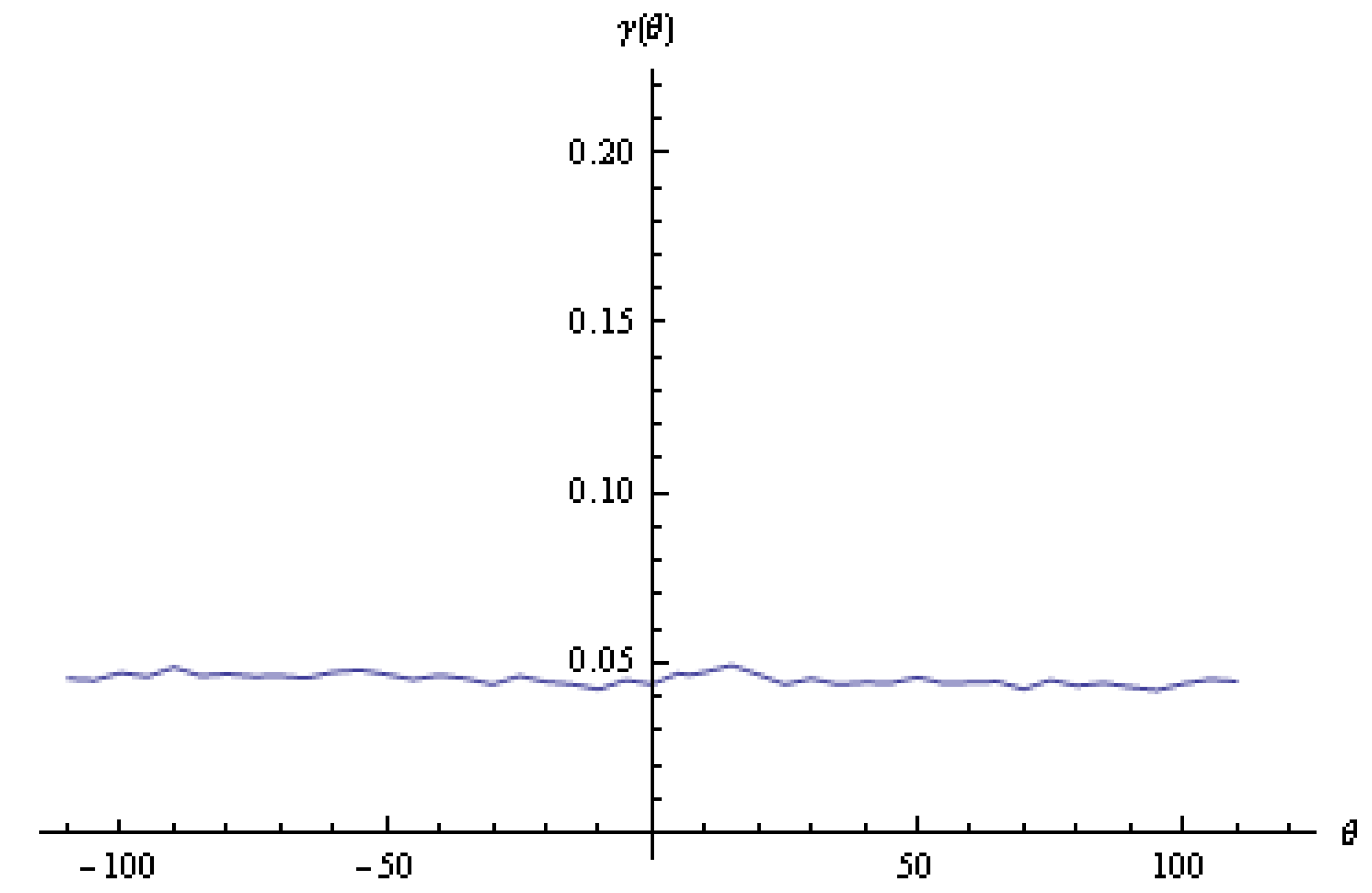
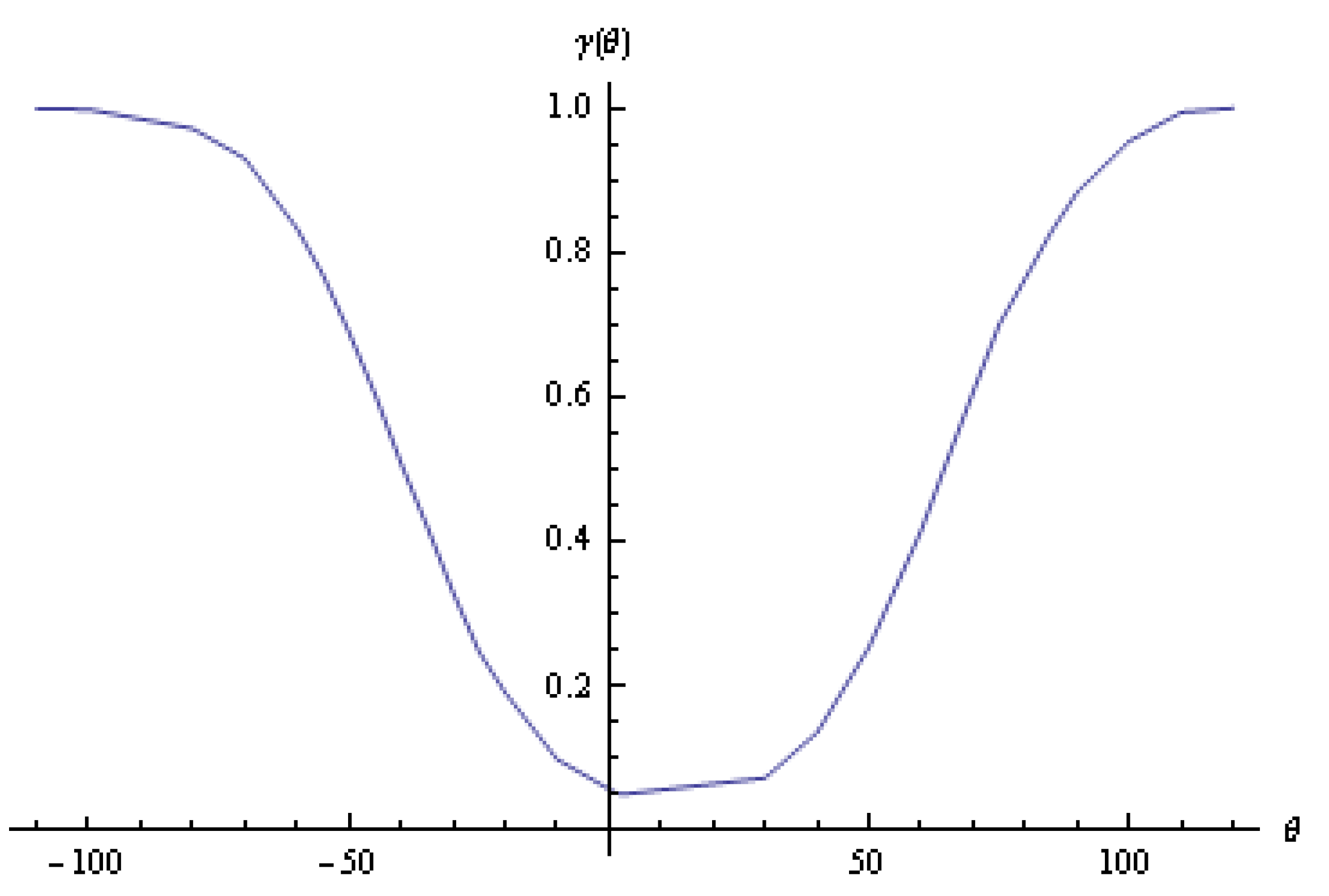
From Table 4, we can see that the values of $\gamma \left({\theta }_1\right)$ depended on the value of ${\theta }_1,$ and as the value of ${\theta }_1$ became larger or smaller, $\gamma \left({\theta }_1\right)$ approached 1. On the other hand, Table 5 shows that the values of $\gamma \left({\theta }_1\right)$ oscillated around $0.05$ and did not depend on ${\theta }_1.$ Thus, the Bayesian predictive distribution was better in predicting future data than the Wald predictive distribution.

To check the validity of the power of a test, plots of $\gamma \left({\theta }_1\right)$ versus ${\theta }_1$ are shown in Figure 1 and Figure 2 for the Bayesian predictive-distribution approach and the Wald predictive-distribution approach, respectively.

Figure 1. The power function $\gamma \left({\theta }_1\right)$ for the Bayesian predictive-distribution approach.

Figure 2. The power function $\gamma \left({\theta }_1\right)$ for the Wald predictive-distribution approach.

5. Application

In this section, we present an application of making a prediction using Bayesian predictive density about a future statistic based on a past sufficient statistic calculated from a real data set. In this application, we consider data set number 139 from [38], which represents the measurements $L_i$ of the length of the forearms (in inches) taken from 140 adult males. The distribution of this data set is normal, with mean $18.8$ and variance $1.25546$; $L_i\sim N(18.8,1.25546),i=1,2,\dots ,140.$

By using the following transformation,

$$X_i=\frac{L_i-18.8}{1.12047}+\theta ,$$

we transform this data set to $N(\theta ,1).$

The following data comprise a random sample of size 18 taken from the original transformed data to $N(\theta ,1),$ when $\theta =2.5$:

$$\begin{array}{llllll}3.12282\hfill & 2.58734& 3.92605\hfill & 2.67658& 1.78410& 1.9626\\ 0.26689\hfill & 1.69486& 2.94433\hfill & 2.23034& 3.30132& 2.23034\\ 2.49809\hfill & 4.37229& 1.33786\hfill & 3.39057& 1.15937& 0.534634.\end{array}$$

From this data set, the value of the past sufficient statistic $w=\sum x_i=42.0204.$ At significance level $\alpha =0.05,$ we want to test the hypothesis,

$$H_0:d(g,h)=0\mathrm{versus}{H}_1:d(g,h)>0.$$

As all divergence measures give the same decision regarding the hypothesis testing in (24), we use the Kullback–Leibler divergence measure in (1) to calculate the distance d between the classical distribution g and the Bayesian predictive distribution h.

The value of $d_{cal}^{\ast }=0.0741083,$ and from the percentiles Table S1, we obtain $d_{tab}=6.77810$; as can be seen, $d_{cal}^{\ast }<d_{tab}$. Furthermore, the value of ${\overline{d}}_{cal}^{\ast }=2.64472,$ and from the percentiles Table S2, we obtain ${\overline{d}}_{tab}=2.78029;$ as can be seen, ${\overline{d}}_{cal}^{\ast }<{\overline{d}}_{tab}$. Thus, the decision is to fail to reject $H_0$. In other words, it is appropriate to use the Bayesian predictive distribution to predict the sum of the forearm lengths of males. As a result, we can predict the average length of forearms for males in general.

6. Conclusions

In this article, the Bayesian and Wald predictive distributions of future statistic V based on past sufficient statistic W from normal density were derived. Several divergence measures were used as criteria to obtain the distance between the classical distribution of future statistics and each of the Bayesian and the Wald predictive distributions. Hypothesis testing was used to test the closeness between the classical and each of the Bayesian and the Wald predictive distributions. The simulation results showed that all divergence measures used in this paper gave the same decisions in all cases. Therefore, it is recommended to use a divergence measure with simpler computations. Based on the power of a test, we conclude that Bayesian predictive distribution is better than Wald predictive distribution in normal distribution cases.