Single-View 3D Reconstruction via Differentiable Rendering and Inverse Procedural Modeling ^†

Abstract

Three-dimensional models, reconstructed from real-life objects, are extensively used in virtual and mixed reality technologies. In this paper we propose an approach to 3D model reconstruction via inverse procedural modeling and describe two variants of this approach. The first option is to fit a set of input parameters using a genetic algorithm. The second option allows us to significantly improve precision by using gradients within the memetic algorithm, differentiable rendering, and differentiable procedural generators. We demonstrate the results of our work on different models, including trees, which are complex objects that most existing methods cannot reconstruct. In our work, we see two main contributions. First, we propose a method to join differentiable rendering and inverse procedural modeling. This gives us the ability to reconstruct 3D models more accurately than existing approaches when few input images are available, even for a single image. Second, we combine both differentiable and non-differentiable procedural generators into a single framework that allows us to apply inverse procedural modeling to fairly complex generators. We show that both variants of our approach can be useful: the differentiable one is more precise but puts limitations on the procedural generator, while the one based on genetic algorithms can be used with any existing generator. The proposed approach uses information about the symmetry and structure of the object to achieve high-quality reconstruction from a single image.

1. Introduction

Modern computer graphics applications require an extensive range of 3D models and textures to populate virtual environments. First of all, we see an increasing demand for realistic virtual content in the growing game and movie industries. The popularity of virtual and augmented reality also enforces this demand. Manual creation of all models requires much time and resources. A significant part of virtual content is created from real-life objects via 3D reconstruction, which remains one of the most important tasks at the intersection of computer vision and graphics. In recent years, we have also seen increased interest in procedural model generation and representation. Sophisticated procedural generation tools are being implemented in game engines. The procedural approach also has other advantages:

• Procedural models are editable, semantically meaningful, and often can be animated;
• A mesh obtained from such models has high-quality triangulation;
• Procedural models are memory-saving compared to other 3D representations.

Despite the known advantages of procedural models, their creation remains a predominantly manual process. Reconstruction of objects using procedural models can speed up their creation, simplify subsequent modification of models, and bring other advantages of the procedural approach to the field of 3D reconstruction. This is why a 3D reconstruction method that creates procedural geometry is badly needed. However, the intersection of these two groups of methods (3D reconstruction and procedural generation) remains relatively unexplored.

Typically, a combination of different approaches is employed, when generated or reconstructed models are further refined by artists. This is especially common in video games, as each model in the game is not only a 3D mesh with a set of textures, but also a more complex object with various levels of detail, animation, physics, etc. 3D reconstruction is a fundamental task in computer vision and numerous methodologies have been proposed over the past decades. To achieve high-quality 3D geometric reconstruction, scanners or LIDARs are the most optimal solution, provided the necessary equipment is available. Image-based approaches are much easier to use and will be the topic of this paper. In recent years, deep learning methods, such as NeRF [1], have made remarkable progress in solving the new problem of view synthesis. Although NeRF and its successors are good at capturing details, they require a significant amount of time and many input images. Other deep learning methods, such as [2,3], focus on 3D reconstruction from a single image, but their results are unlikely to be applicable due to low quality. Additionally, it should be noted that deep learning methods rely on an implicit representation of the model in neural network weights, and extracting the actual mesh and textures from it becomes a challenging task [4,5].

Differentiable rendering is a promising and rapidly developing approach to 3D reconstruction [6]. It enables gradient-based optimization of scene parameters, such as vertex positions and textures, to achieve a better match with the input images. One application of differentiable rendering is the reconstruction of complex materials’ Bidirectional Reflectance Distribution Functions (BRDFs). Although differentiable rendering can be used with implicit representations such as signed distance functions (SDF) [7], most approaches use a classical mesh-textures representation, which is more user-friendly than deep learning methods.

Despite the progress made in the field of image-based 3D reconstruction in recent years, there are still significant obstacles preventing the wider adoption of these methods in practical applications. First, performing high-quality reconstruction requires a significant number of images ([6] uses 100 images to achieve high quality). Single-view reconstruction methods are barely applicable, while others often require dozens of images of different views. Second, even the best approaches struggle to reconstruct complex objects with many thin parts, such as trees and other vegetation. The key point is that an exact reconstruction of every small branch and leaf is not necessary; rather, the model should be sufficiently detailed and visually similar to the given reference. The third and, perhaps, the most significant problem of reconstruction is the difficulty of editing the resulting models. Typically, these methods create one large triangular mesh that lacks information about the structure of the object, such as which branch a particular triangle belongs to in the tree model. Artifacts in the resulting model are also a serious problem, often requiring regularization or post-processing techniques to reduce them.

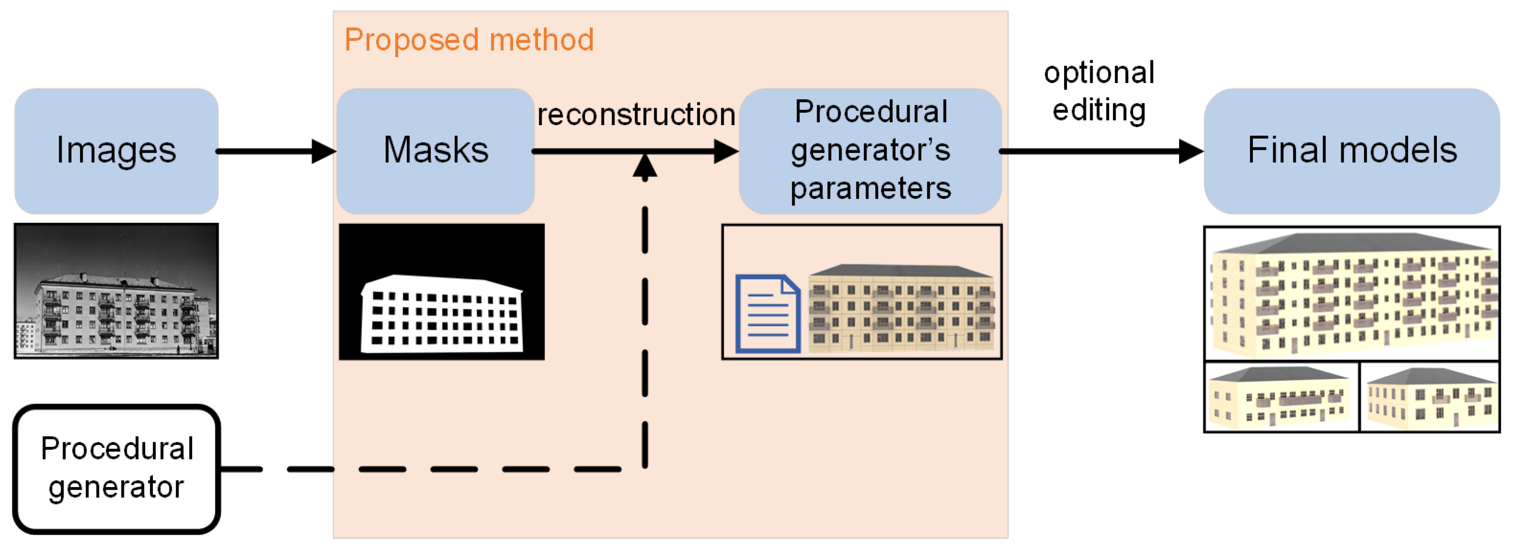
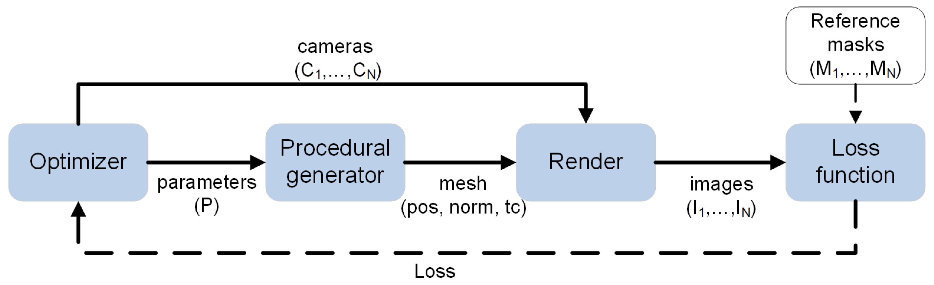
Most image-based reconstruction methods do not take into account an important aspect of applications and human perception: the structure of an object. Modification is often required to use the reconstructed model, and lack of structural information makes any modifications much more difficult. Procedural generation is an alternative method for obtaining 3D models, consisting of rules that establish a correlation between input parameters and 3D objects of a certain class. In this paper, we propose a novel approach that utilizes procedural generation for single-view and multi-view reconstruction of triangular meshes. Instead of directly estimating the position of mesh vertices, we estimate the input parameters of the procedural generator through a silhouette loss function between the reference and rendered images, using differentiable rendering and creating partially differentiable procedural generators for gradient-based optimization. Our approach also allows us to conveniently modify/edit the model by changing the estimated input parameters, such as creating new levels of detail, altering the geometry and textures of individual mesh parts, and more. In summary, the contributions of this work are outlined as follows:

• An algorithm for single-view 3D reconstruction using procedural modeling is proposed. Unlike many other methods, it produces an editable 3D procedural model that can be easily converted in high-quality mesh grids and arbitrary levels of details.
• To obtain an editable 3D procedural model as a reconstruction result, two procedural modeling approaches were studied: non-differentiable and differentiable. The first approach is easier to implement for a wider range of tasks, while the second can be used to obtain more precise reconstruction.
• Our model outperforms modern single-view reconstruction methods and shows results comparable to state-of-the-art approaches for multi-view reconstruction (it demonstrates IoU metrics more than 0.9 for most models with the exception of extremely complex ones).

It should be noted that symmetry is a key property that allows one to reduce the dimension of phase space. Thanks to this property, high-quality optimization of an object is possible using just one image. For real-life objects that do not have symmetry our method also works, but it performs only an approximate reconstruction. However, even in this case the resulting 3D object does not have artifacts typical of most other reconstruction methods.

This work generalizes and extends the results presented at the conferences [8,9]. The novelty of this work is that we propose a general approach for both differentiable and non-differentiable procedural generators as well as an intermediate case when only several parameters of procedural generator are differentiable (for example, the case of buildings). In addition to the conference papers, we performed an extensive comparison and showed the benefits of the proposed approach on different types of procedural generators and 3D models. Finally, we showed that for inverse procedural modeling, it is enough to apply differentiable rendering to a silhouette image only. This, in algorithmic terms, significantly reduces computational complexity and allows us to use simpler and lighter-weight approaches to differentiable rendering (Section 4.4).

The remainder of this paper is organized as follows. Section 2 describes other reconstruction methods and related studies, including inverse procedural modeling, which we consider to be closest to the topic of this research. The proposed method is introduced in Section 3. Section 4 discusses the implementation and demonstrates the results of the proposed approach. Finally, Section 5 outlines the discussions and conclusions.

2. Related Works

Our work joins together ideas from several areas. They are 3D model reconstruction, neural and differentiable rendering, and forward and inverse procedural modeling. In the following, we describe what has already been accomplished before us in these areas and finalize motivation for our research in Section 2.7.

2.1. Three-Dimensional Reconstruction

Multi-view 3D geometry reconstruction has been well studied in the literature. Traditional and well-developed approaches to solve this task include structure from motion (SfM) [10] for large-scale and high-quality reconstruction and mapping (SLAM) [11] for navigation. Although these approaches are capable of providing high-quality results, they have two significant limitations. First, they are unable to reconstruct the unseen parts of objects and therefore require a large number of input images. Secondly, they have difficulty working with non-Lambertian or textureless objects.

Consequently, there is a growing trend towards learning-based approaches that leverage shape priors learned from the data by considering one or few images. These methods use different scene representations, such as meshes [12,13,14], voxel grids [15,16], point clouds [17,18], or implicit functions [19]. Among these methods, mesh reconstruction is especially important for our work. Most single-view 3D mesh reconstruction methods use an encoder–decoder architecture, in which the encoder extracts features from the image and the decoder deforms an initial mesh to match the target shape. It is worth noting that these methods are trained and evaluated on the same object categories. However, recent work [20] has shown that these approaches primarily achieve recognition rather than reconstruction when working with a single image. Although there have been several works on generalized single-view 3D reconstruction [3,21], models reconstructed from a single image using these methods often lack the quality required for practical applications. However, a study recently published dealing with 3D reconstruction using Gaussian splatting [22] shows very promising results along with a higher generalization ability.

2.2. Differentiable Rendering and Neural SDF

The field of physically based differentiable rendering [6,23,24,25,26] is an active area of research related to the accurate reconstruction of 3D models and materials. These algorithms provide gradient information for the loss function with respect to scene parameters, which can be minimized using gradient descent. The choice of scene representation is crucial for these approaches, with the mesh-based representation being the most extensively studied. Specific regularization techniques [27] and modifications of the Adam optimizer [28] were proposed to improve the quality. Recent work by Nicolet et al. [29] has made significant advances in this area by improving the quality of the resulting meshes. Other scene representations, such as differentiable signed distance functions (SDFs) [30], have also been explored. Differential rendering can also be combined with deep learning [3] to provide face quality supervision and regularization. However, these approaches typically require a large number of input images, which is difficult to obtain in practice. Particular mention should be made of the work [31] which, in our opinion, is a kind of precursor of approaches based on differentiable rendering. In this work, the minimum area surface that best fits the input data and suitable priors is computed as a solution to a variational convex optimization problem.

2.3. NeRF

While mesh-based or surface-based representations offer efficient rendering and easy-to-use models, optimizing surface geometry using image-based methods can be challenging due to non-convexity. Volumetric representations [32,33] can reliably achieve a desirable minimum, but are usually unable to capture finer details. Alternatively, point-based shape representations have been shown to produce high-quality scene reconstructions [34,35].

Another useful technique for scalable scene representation is the use of coordinate-based neural networks, which are commonly known as neural fields [36,37,38]. Neural fields extend the resolution limits of discrete grids and generalize to higher-dimensional signals, including directional emission [36]. Neural fields [38] have demonstrated the ability to handle complex scenes and produce compelling results in seconds. However, for practical use, these results often need to be converted into a 3D mesh, since most rendering engines primarily work with meshes. This conversion can be challenging and result in sub-optimal models with more triangles and lower visual quality [38]. Another major disadvantage of NeRF is the same as for approaches based on differential rendering—it requires a large number of input images. Compared to pure differentiable rendering approaches, NeRF-based methods are more stable and do not require specific initial conditions for optimizations, but produce models that are much more demanding in memory consumption and computational power to render them directly.

2.4. Procedural Modeling

Procedural generation is a widely used approach to create a variety of virtual content. It can be used at different levels, from individual objects to large-scale open worlds and game scenarios [39,40]. Typically, a procedural object generator works as a function that transforms a vector of numerical parameters into a 3D mesh of a certain class, for example, trees or buildings. Procedural modeling of trees is of particular interest because creating detailed vegetation by hand is especially hard and tedious. Projects like SpeedTree [41] provide an artist with a tool that allows them to interactively create highly detailed tree models, while stand-alone procedural generators [42,43] create a plant model without human involvement based on a set of input parameters. Due to its complexity, traditional 3D reconstruction of a tree model is much more difficult, since many details are hidden by foliage. Considering this, and the fact that procedural generators are capable of producing high-quality tree models, a few specialized tree reconstruction methods using procedural generators have been proposed.

2.5. Inverse Procedural Modeling

The work [44,45] proposes inverse procedural generation, that is, selecting generator parameters based on the input 3D tree model to recreate it using the generator. Thus, the procedure takes a polygonal tree model as input. Tree sampling was performed using Markov chain Monte Carlo in parameter space. The main limitation of this work is that a 3D mesh is already required as input. The SIGGRAPH course [46] provides a comprehensive review of inverse procedural modeling based on already existing 3D content. However, procedural-based reconstruction from one or a few images remains an open problem in general.

To move from 3D modeling to a 3D reconstruction problem, it is necessary to propose a similarity metric that answers the following question: “To what extent does a given set of procedural generator parameters allow one to obtain a model similar to the input reference?”

This strategy was adapted in [8,47]. The work [47] analyzes an input tree image and infers a parametric L-system that represents it. In [8], the authors use more complex stochastic procedural models that simulate the process of vegetation growth, so the selection of procedural generator parameters is carried out using genetic algorithms. Both methods take a single tree image and find the optimal generator parameters by minimizing the loss function between a given reference and the model image created by the generator. Despite relatively good results, these methods are specific for plants (especially [47]) and cannot be applied to a wider class of objects.

There are several works devoted to inverse procedural modeling of specific classes of objects, such as materials [48], facades [49], and knitting yarn [50,51]. Reference [49] derives a so-called “split grammar” for a given facade layout. A more general approach has also been studied. In the work [52], the authors focus on an interactive procedural generation tool that allows for greater user control over the generated output. The user then modifies the output interactively, and the modifications are passed back to the procedural model as its parameters by solving the inverse procedural modeling problem.

2.6. Adding Geometric Constraints

There are a number of methods focused on the reconstruction of objects with geometric constraints, such as bodies of revolution [53,54], buildings [55], human bodies [56,57], etc. These approaches are carefully designed for specific application scenarios and specific input data. They may use [55], or not use learning-based approaches. These approaches usually provide sufficiently accurate results for the intended applications. However, they are more limited and specific to a certain type of object than the procedural approach in general.

2.7. Motivation for Our Work

Most of the works devoted to 3D reconstruction tend to overlook how the reconstructed model can actually be used. Even if a method is able to produce a decent triangle mesh, it will likely need to be modified to remove some artifacts and adjust it to specific users’ needs. This process is much more complex with methods based on implicit representations such as NeRF [36] or Gaussian Splatting [58], which requires additional steps [5,59]. In most cases, models have to be converted to a mesh or point cloud, which likely reduces quality.

Also, in the gaming and movie industries models are often further edited to match a specific visual style and sometimes a set of similar models is created from a single real-world object. This shows that even perfectly reconstructed models often need editing to meet the requirements of the end user and how easy it is to carry out such editing largely determines the applicability of a particular method. High-level editing, such as increasing the number of floors or replacing windows in a building, require much effort unless we have access to information about the structure of the object and the ability to change it directly.

There are ideas of procedural generation and inverse procedural generation, that is, describing an existing 3D model with the parameters of a procedural generator [44,45]. The main reason for this is the change in the model structure through its parameters. This observation leads us to the idea of inverse procedural generation, which uses images as input instead of an existing model. This approach allows us to reconstruct the structure of the object and greatly simplifies further modifications.

3. Proposed Method

In this section we describe our method for single- and multi-view 3D reconstruction using procedural generation. We first present our general reconstruction pipeline and its two variants: differentiable and non-differentiable. The advantages and limitations of the differentiable variant are discussed. We then present procedural generators used in our work and discuss the differences between them when used for reconstruction. The next part of this section is dedicated to the optimization process in both differentiable and non-differentiable pipelines.

3.1. Workflow

In our work, we assume that we are given a set of N images $R_i$ of the same object from different (and unknown) viewpoints. We do not use reference images directly, but instead use “masks” $M_i$ taken from these images. The exact type of mask depends on the procedural generator, but in most cases it is simply a binary mask separating the object from the background. This allows us to ignore the lighting in the original image and simplifies the calculation of the loss function during the optimization process. Figure 1 shows the general workflow of our proposed method.

Figure 1. General workflow of proposed method. Binary masks are generated from input images and used to reconstruct 3D models in form of procedural generator’s input parameters. Then, this set of parameters can be optionally edited and/or used to create a group of similar models.

Creating a mask remains beyond the scope of consideration in this paper, and any existing segmentation algorithms can be used for this. Masks obtained in one way or another are used by our algorithm to remove from the loss function influence of insignificant details, which is visible in the input image.

3.2. Reconstruction Pipeline

We assume that we already know the procedural generator $Gen$ needed for reconstruction, either because it was chosen manually or through some classification. It takes a set of parameters P to create a triangle mesh consisting of vertex positions, normals, and texture coordinates $Gen\left(P\right)=Mesh=\{po{s}_i,nor{m}_i,t{c}_i\}$, where $po{s}_i$ is the vertex position, $nor{m}_i$ – vertex normal, and $t{c}_i$ is the vertex texture coordinates of i-th vertex. A mask of this mesh can then be created using a render function that takes only vertex positions $pos$ and camera parameters C: $I=Render(Mesh,C)$. We perform the reconstruction as an optimization of the loss function between the given and rendered masks:

$$Loss(P,C_1,\dots ,C_N)=\frac{1}{N}\ast \sum _{i=1}^{N}MSE(I_i,M_i)=\frac{1}{N}\ast \sum _{i=1}^{N}MSE(Render(Gen\left(P\right),C_i),M_i)$$

(1)

Then, the goal of our algorithm is to minimize the loss function and find the optimal parameters of the generator $P^{\ast }$ and cameras $C_1^{\ast },\dots ,C_N^{\ast }$. This brings us to the general reconstruction pipeline shown in Figure 2.

Figure 2. The mesh reconstruction cycle consists of a procedural generator that creates a mesh from the input parameters, which is then rendered as a mask. A loss function is calculated between it and the reference image mask. The loss value is then returned to the optimizer that updates the parameters of the generator and cameras.

This general reconstruction pipeline looks simple and straightforward, especially since it treats the procedural generator as a black box function that is able to create a 3D model from a set of parameters. This fact allows us to use any existing procedural generator without knowing how it actually works internally, at least in theory, since we still need to know which input parameter values are correct and which are not. However, in this case we need to implement a gradient-free optimization method for the loss function (1), which can pose a serious problem. Later, we will describe the cases where we have to use this general pipeline and show how to make optimization for it relatively efficient. However, in most cases we can make a few changes to this pipeline that will allow for gradient-based optimization. This requires gradients of the loss function with respect to the scene parameters. Using a differentiable renderer to render the mask and calculate the loss function, we can obtain $\frac{dLoss}{dC}$, where C represents camera parameters. Our implementation can use Mitsuba 3 [60] or our own differentiable renderer for this purpose. Obtaining $\frac{dLoss}{dP}$ (where P represents the procedural model parameters) is a little more complicated. Given the chain rule and suppose that the mask does not depend on the model normal vectors and texture coordinates, we obtain:

$$\frac{dLoss}{dP}=\frac{dLoss}{dpos}\ast \frac{dpos}{dP}$$

(2)

The equation term $\frac{dLoss}{dpos}$ (where $pos$ is the vector of all vertex positions) also comes from the differentiable renderer, and the Jacobian $\frac{dpos}{dP}$ must be obtained from the procedural generator. The whole process of optimizing the silhouette loss function is shown in Figure 3. Creating a procedural generator capable of calculating $\frac{dpos}{dP}$ is the most important part of this improved pipeline. We would call a generator that can do this a differentiable procedural generator. In the next section we describe the differentiable procedural generators created for this work and the challenges they pose. In fact, most non-trivial generators can only be partially differentiable, and we address this issue in the third section, where the optimizer is described in details.

Figure 3. Gradient-based reconstruction pipeline. Rendering and loss function calculation are performed by a differentiable renderer. Assuming that the rendered mask depends only on the vertex positions $pos$, and not on the normals and texture coordinates, we obtain $\frac{dLoss}{dC}$ and $\frac{dLoss}{dpos}$. Then, to obtain $\frac{dLoss}{dP}$, the procedural generator must be able to compute the Jacobian $\frac{dpos}{dP}$ alongside with the mesh $(pos,norm,tc)$.

3.3. Differentiable Procedural Generators

The previous section introduced a pipeline that treats the procedural generator as a black box function capable of producing a mesh $(pos,norm,tc)$ (where $pos$, $norm$, and $tc$ are position vectors, normals, and texture coordinates) and the Jacobian $\frac{dPos}{dP}$ from the input vector P. However, it is impossible to create a generator for nontrivial objects that functions as a smooth differentiable function due to the discrete properties of the objects, such as, for example, the number of floors in a building. For consistency, we still include these parameters in the vector P, assuming that $\frac{dPos}{d{P}_d}=0$ for each parameter $P_d$ of this type.

In this work, we have developed two different procedural generators: one for dishes, and the other for buildings. Both generators were created from scratch using the automatic differentiation library CppAD [61], which helps us to obtain the required derivatives from computational graphs without explicitly calculating them in our code. The dish generator is an example of a simple and easily differentiable algorithm that has only one binary parameter. It has axial symmetry. It defines a spline that forms the boundary of the object along the Y axis. Further generation of the 3D object occurs by rotating the spline around the Y axis. Algorithm 1 shows the high-level pseudocode for the dish generator.

Algorithm 1 Differentiable dishes generator.

P—input parameters, $LOD$—level of detail Result: $Mesh=\{po{s}_i,nor{m}_i,t{c}_i\}$—3D model $splineParams,hasHandle,handleSplineParams\leftarrow P$ $spline\leftarrow getSpline\left(splineParams\right)$ $transoformSpline(spline,LOD)$ $baseModel\leftarrow getBaseModel(spline,LOD)$ if hasHandle then     $handleSpline\leftarrow getSpline\left(handleSplineParams\right)$     $transoformHandleSpline(handleSpline,LOD)$     $handleModel\leftarrow getHandleModel(handleSpline,LOD)$     return $baseModel\cup handleModel$          ▹ Concatenate lists of vertices end if return $baseModel$

In contrast, the building generator was designed to demonstrate the capability of our method to handle generators with multiple discrete features. Algorithm 2 shows its pseudocode. The building generator has several symmetry planes: XY and YZ. At the same time, there is also symmetry relative to the XZ plane, but only at the level of one floor because in general the floors are not the same. Thus, the symmetry of the object is intensively used to reduce the dimension of the phase space and makes possible high-quality optimization of the object from a single image. Both generators are capable of producing a significant variety of models based on input parameters (Figure 4) and are capable of creating different levels of detail for each model (Figure 5).

Algorithm 2 Differentiable buildings generator.

P—input parameters, $LOD$—level of detail Result: $Mesh=\{po{s}_i,nor{m}_i,t{c}_i\}$—3D model $windowParams,balconyParams,roofParams,structureParams,floors,sections\leftarrow P$ $windowModel\leftarrow getWindow(windowParams,LOD)$ $balconyModel\leftarrow getBalcony(balconyParams,LOD)$ $wallPatch\leftarrow getWallPatch(windowModel,balconyModel,structureParams)$ $roofSection\leftarrow getRoof(roofParams,LOD)$ $buildingModel\leftarrow ⌀$ for $i\leftarrow 1,sections$ do     $sectionModel\leftarrow ⌀$     for $j\leftarrow 1,floors$ do         $sectionModel\leftarrow sectionModel\cup moveFloor(wallPatch,j)$     end for     $sectionModel\leftarrow sectionModel\cup roofSection$     $buildingModel\leftarrow buildingModel\cup moveSection(roofSection,i)$ end for return $buildingModel$

Figure 4. Some examples of models created with dish (top row) and building (bottom row) generators.

Figure 5. Levels of detail for dish (top row) and building (bottom row) generators.

3.4. Gradient-Based Optimization

Even the simple procedural models demonstrated in the previous section prove to be extremely difficult to optimize functions for due to two factors: the large number of nonlinear internal dependencies within the generator and heterogeneous input parameters, some of which are integers with a limited set of possible values. Our first attempt at 3D reconstruction using procedural generators [8] relied on a specific implementation of a genetic algorithm [62] to find solutions without gradient calculation, but only for a limited set of problems. The ability to calculate the gradient of the loss function expands the range of available optimization methods. However, it is not yet possible to obtain derivatives with respect to parameters reflecting discrete features of the procedural model.

To address this issue, we implemented a memetic algorithm [63], which combines a genetic algorithm with gradient-based optimization. The algorithm starts with an initial population—a set of initial parameter values obtained from predefined presets. Each preset consists of input parameters representing an adequate model (as shown in Figure 4). The memetic algorithm performs random mutations and recombination of the original population in addition to gradient-based optimization. It works with a medium-sized population of a few hundred individuals and uses tournaments to match partners for crossover. At each iteration, all but a few best individuals from the old population are replaced by new ones. Although this process requires several hundred iterations, it can be performed with low levels of detail and low rendering resolution. To further improve quality, the solution obtained by the memetic algorithm is used as an initial approximation for a subsequent round of gradient-based optimization with a higher level of details and higher rendering resolution. The results at each step are shown in Figure 6.

Figure 6. Results of model reconstruction after each optimization step. From left to right: reference image, genetic algorithm with rendering resolution 128 × 128, and gradient descent with resolution 256 × 256 and 512 × 512, respectively.

3.5. Non-Differentiable Case

Using differentiable rendering and procedural generation allows us to use gradient descent and makes optimization much easier, even with integer input parameters that should be optimized differently. However, some types of procedural generators are not suitable for the described pipeline. Modern systems for automatic plant modeling, such as [43,64,65], focus on simulating the growth process and the influence of the environment on it. This kind of simulation is crucial for a more realistic result, but at the same time it makes the creation process more random and less stable. We implemented a generator based on the work [43] and found that even a tiny change in the input parameters for it can lead to a significantly different tree structure. The overall tree shape remains the same, but the exact location of the individual branches changes. In this case it is extremely difficult to obtain meaningful gradients using automatic differentiation. The same problem appeared to some extent in the much simpler rule-based generator [66]. So, tree modeling shows the limitations of the differentiable reconstruction approach, but it is still possible to perform reconstruction using the general pipeline (Figure 2). Since we cannot obtain the gradients of the loss function in this case, we used a genetic algorithm from our previous work. A special loss function was also used for the reconstruction of tree models.

3.5.1. Tree Similarity Function

We define a loss function between the generated tree model and the reference image based on the tree similarity function and an optional set of regularization multipliers (factors).

$$Loss=TSim\ast \prod _{c\in C}\frac{min(c,c_{ref})}{max(c,c_{ref})}$$

(3)

The tree similarity value is obtained by comparing the reference image with the impostors of the generated tree model. To facilitate this comparison, semantic masks are used, in which each pixel is assigned one of three categories: branch, foliage, or background. One method for obtaining such a mask from the source image is to use a neural network, as discussed in [67]. In simpler cases, the mask can be derived solely from the color of the pixel, with green representing the leaves and brown or gray representing the branches and trunk. The reference and generated images are divided into 20–30 narrow horizontal stripes, for each of which the following are determined:

• $[a_i,d_i]$—crown borders;
• $[b_i,c_i]$—dense crown borders (>75% leaf pixels);
• $B_i$—percentage of branch pixels;
• $L_i$—percentage of leaf pixels.

According to the ratio $B_i/L_i$, each stripe belongs to either the crown or the trunk, see Figure 7. By comparing the parameters $a_i$, $b_i$, $c_i$, $d_i$, and the ratio $B_i/L_i$ for each stripe of the reference image and the generated image, the tree similarity value ($TSim$) can be calculated.

Figure 7. Original image, semantic mask, visualization of division into stripes. Brown stripes correspond to the trunk, green stripes correspond to the crown. The vertical lines inside each stripe are the values $a_i$, $b_i$, $c_i$, and $d_i$, respectively.

To guide the optimization process, regularization factors $\frac{min(c,c_{ref})}{max(c,c_{ref})}$ are introduced. These multipliers are determined based on the minimum and maximum values of certain characteristics, such as the number of vertices in the branch graph, height and width, average density of branches and leaves, and average leaf size. Although none of these characteristics are mandatory, it is recommended to specify the number of vertices in the branch graph to avoid searching for a solution among models with excessively high geometric complexity, which could slow down the search process.

3.5.2. Genetic Algorithm Implementation

The previously mentioned similarity function is used as the objective function in the genetic algorithm. The proposed method consists of several elementary genetic algorithms, and the best result is selected from each elementary algorithm. Each elementary genetic algorithm involves the initialization of a population and its evolution over a fixed number of generations. In a tree-like population structure, each node represents an elementary genetic algorithm. The algorithms on the leaves of the tree start with a randomly initialized population, while all other algorithms form a population consisting of the fittest individuals obtained from the child nodes. Figure 8 presents the proposed tree-like population structure, where the final result is a small set of the best species at the top level.

Figure 8. Tree-like population structure. An elementary GA of the first level starts with random genes, and GA of level i takes the best species from the last two populations of the previous level. The final result of the whole algorithm is a small set of the best species at the topmost level.

All elementary genetic algorithms follow the same strategy based on the objective function $f\left(x\right)$. At the beginning of each iteration, the half of the population with the lowest fitness value is eliminated. The remaining individuals contribute to the creation of a new generation, with new individuals being created through a one-dot crossover using parents selected from the remaining species of the previous generation. Choice of parents uses fitness proportional selection, meaning that the probability of an individual being chosen as a parent is proportional to its fitness value. The objective function and fitness function are calculated for representatives of the new generation. The mutation chance $M_{chance}$ and the percentage of genes that change $M_{genes}$ are constant.

To increase the chance of meaningful mutations, we introduce a specific mutation procedure, which is shown in the Algorithm 3 below. It is based on pre-collected information about the entire family of objective functions $F=f\left(x\right)$ (each function corresponds to its own input image and set of properties) on a large sample with random input parameters x.

Algorithm 3 Genome quality estimation and mutation.

$ϵ=0.001,B=16,steps=500$ − hyperparameters function Q($i,j$)      using pre-collected pairs $\Pi =\left\{\right(G,f\left(G\right)\left)\right\}$     $P_{i,j}=\#\{f\left(G\right)>ϵ|G\in \Pi ,\frac{j-1}{B}<G_i<\frac{j}{B}\}/\#\Pi$     $P_0=\#\{f\left(G\right)>ϵ|G\in \Pi \}/\#\Pi$     $Q_{i,j}=sign(P_{i,j}-P_0)\ast \frac{max(P_{i,j},P_0)}{min(P_{i,j},P_0)}$     return $Q_{i,j}$ end function function QualityEst(G, N)     $Q={\sum }_{i=1}^{N}Q(i,⌊G_i\ast B⌋)$     return Q end function function Mutation(G, N, $M_{genes}$)▹ genome, genome size, number of genes to mutate     $G_{best}\leftarrow G$     $Q_{best}\leftarrow QualityEst(G,N)$     for $step\leftarrow 1,steps$ do         $k_1,k_2,\dots k_{M_{genes}}=SelectRandomGenes(N,M_{genes})$         $G‘\leftarrow G$         for all $k\in k_1,k_2,\dots k_{M_{genes}}$ do            $G{‘}_k=G{‘}_k+Normal(0,{\sigma }^2)$         end for         $Q‘\leftarrow QualityEst(G‘,N)$         if $Q‘\ge Q_{best}$ then            $Q_{best}\leftarrow Q‘$            $G_{best}\leftarrow G‘$         end if     end for     return $G_{best}$ end function

4. Results

We implemented our method as a standalone program written mostly in C++. Differentiable procedural generators were written from scratch and the CppAD library [61] was used for automatic differentiation inside the generators. We also implemented a differentiable renderer for fast rendering of silhouettes during optimization. We used our own differentiable renderer to reconstruct the models shown here, and Mitsuba 3 [60] was only used for forward rendering of final images.

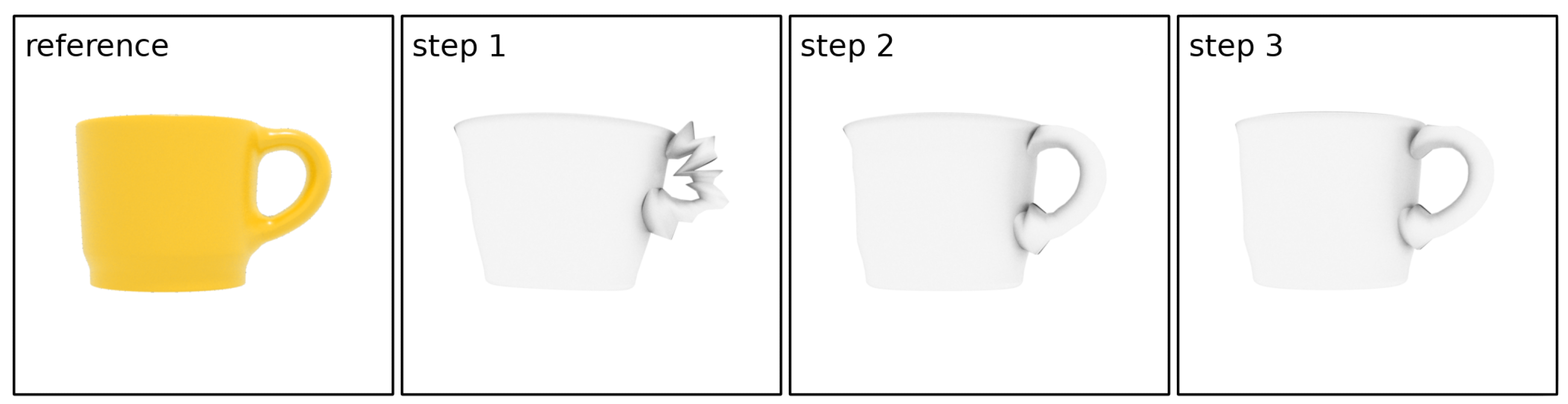
Our method requires defining a set of hyperparameters, such as the number of rendering stages, the size of rendering image, the number of iterations for each stage, and the parameters of genetic or memetic algorithm. We used basically the same set of hyperparameters for all of our results. For reconstruction with differentiable generators, we set the number of optimization stages to 3 or 4 with a rendering resolution 128 × 128 for the first stage and doubled it in each subsequent stage. The memetic algorithm is used only in the first stage with a limit of 5000 iterations; in subsequent stages the Adam optimizer is used with 200–300 iterations per stage. For reconstruction with non-differentiable tree generators, we used only one stage with a rendering resolution of 256 × 256 and a limit of 50 thousand iterations for the genetic algorithm. The whole optimization process takes about 10–20 min with the differentiable procedural generator and up to 30 min with the non-differentiable one. These timings were measured on a PC with AMD Ryzen 7 3700X and NVIDIA RTX 3070 GPU. In general, the implemented algorithm does not place high demands on used hardware. In the experiments described in this section, the program took up no more than 2 gigabytes of RAM and several hundred megabytes of video memory. Our implementation of the algorithm can work on any relatively modern PC or laptop with a GPU.

4.1. Single-View Reconstruction Results

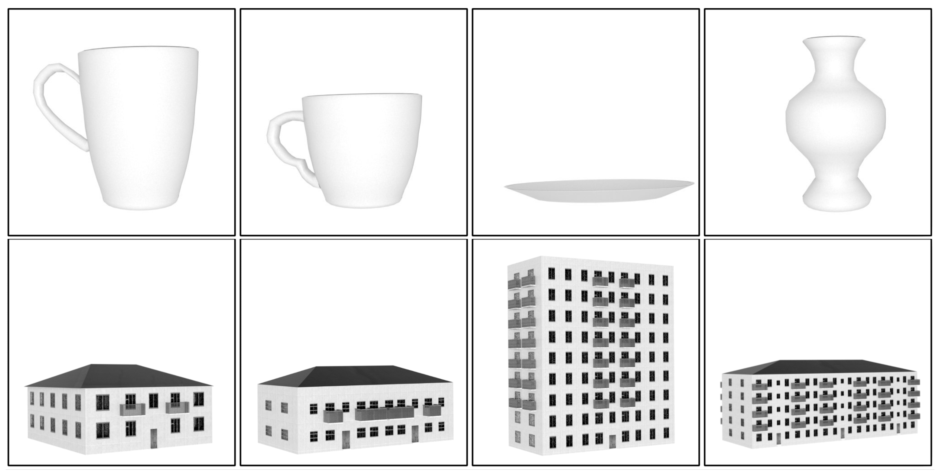
Figure 9 shows the results of single-view reconstruction for different types of objects using the corresponding procedural generators. For building reconstruction, we provided window masks that were created manually, while all other masks were generated automatically. As expected, all presented models are free of usual reconstruction artifacts, are detailed, and have adequate texture coordinates, allowing textures to be applied to them. Reconstruction of the cups and building with differentiable generators results in models very close to the reference ones. The main quality limitation here is the generator itself. The quality of reconstruction with the non-differentiable tree generator is lower because the genetic algorithm struggles to precisely find the local minimum. However, the overall shape of the tree is preserved and the model itself is quite good. Table 1 shows the time required for reconstruction of different models.

Figure 9. Reconstruction results for different types of objects. Differentiable procedural generators were used for cups and buildings and the non-differentiable one for trees. All models were rendered with some default textures whose texture coordinates were provided by the procedural generator.

Table 1. Reconstruction time for different models.

Model	Cup	Bowl	Building	Tree
time (min)	16.3	11.5	19.1	29.0

4.2. Comparison with Other Approaches

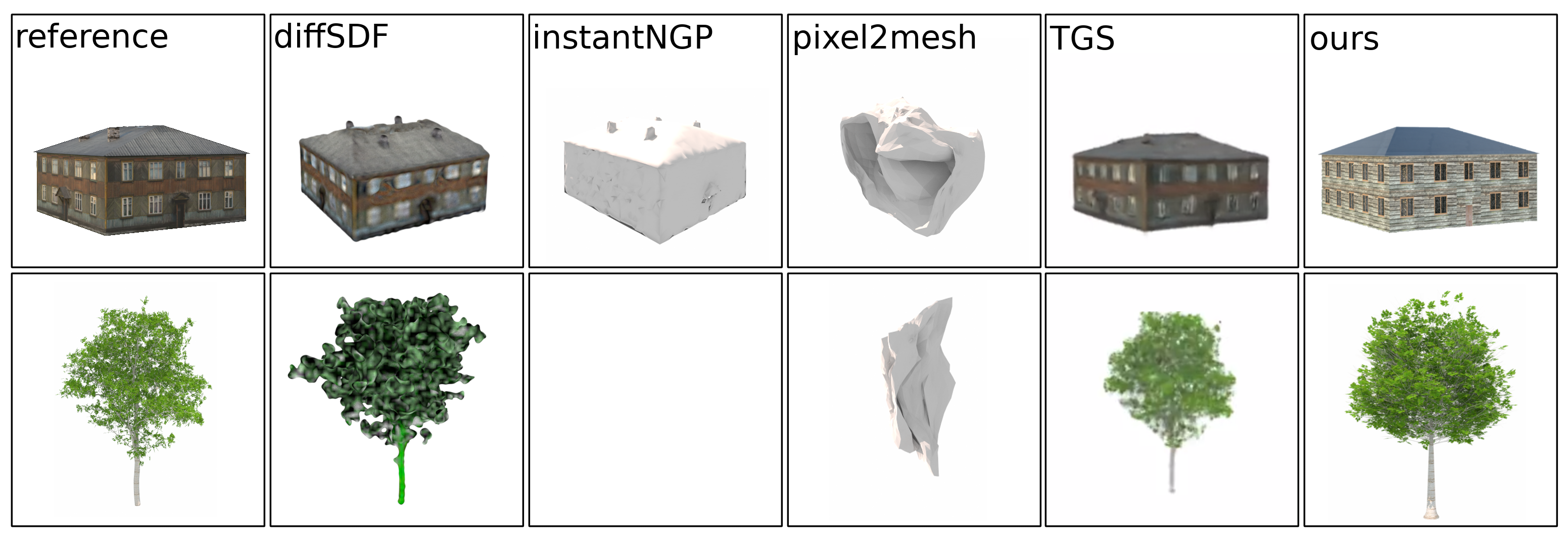
We compared the results of our work with various state-of-the-art image-based 3D reconstruction approaches to demonstrate that our method avoids the problems common to all these algorithms. Four algorithms were used for comparison: InstantNGP, DiffSDF, Pixel2Mesh, and Triplane Gaussian Splatting (TGS). InstantNGP [38] is a modern approach to multi-view reconstruction from NVidia based on the idea of neural radiance fields. It provides the same reconstruction quality as the original NeRF [1], but is an order of magnitude faster. However, it still requires dozens of input images and provides models with various visual artifacts, mainly arising from the transformation of the radiance field into a mesh. DiffSDF [30] is a method that represents a scene as a signed distance field (SDF) and utilizes differentiable rendering to optimize it. It requires fewer input images than NeRF-based approaches and achieves better results for opaque models due to better surface representation. In [30], SDF values are stored in a spatial grid with relatively small resolution. This limits the method’s ability to reconstruct fine details. Pixel2Mesh [12] is a deep neural network capable of creating a 3D mesh from a single image, that does not require training a separate model for every class of objects. TGS [22] is today’s most advanced and powerful approach to single-view 3D reconstruction that highly relies on generative models, such as transformers. It achieves better quality and works faster than previous methods. However, it represents the reconstructed model as a set of 3D Gaussians that cannot be used directly in most applications.

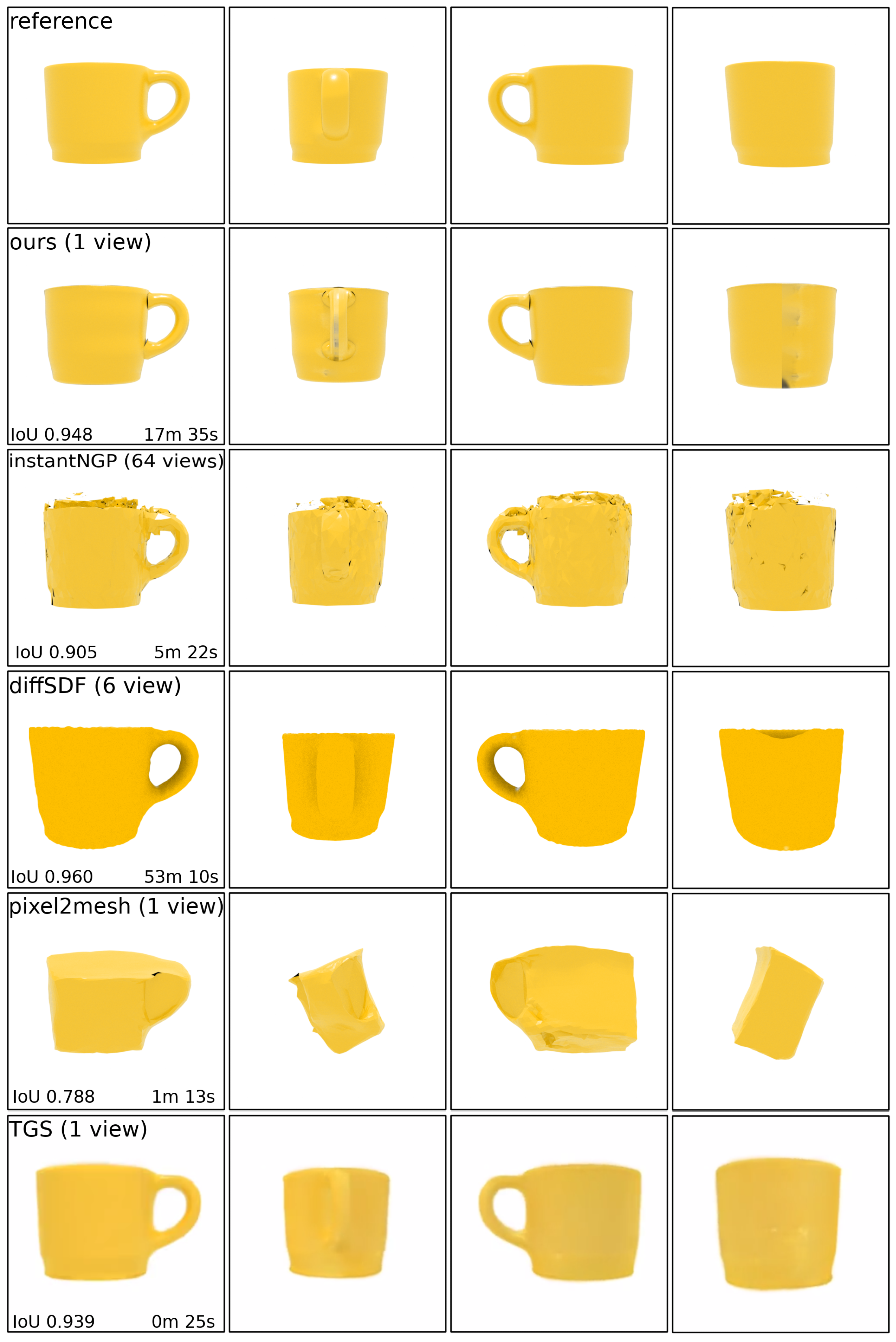
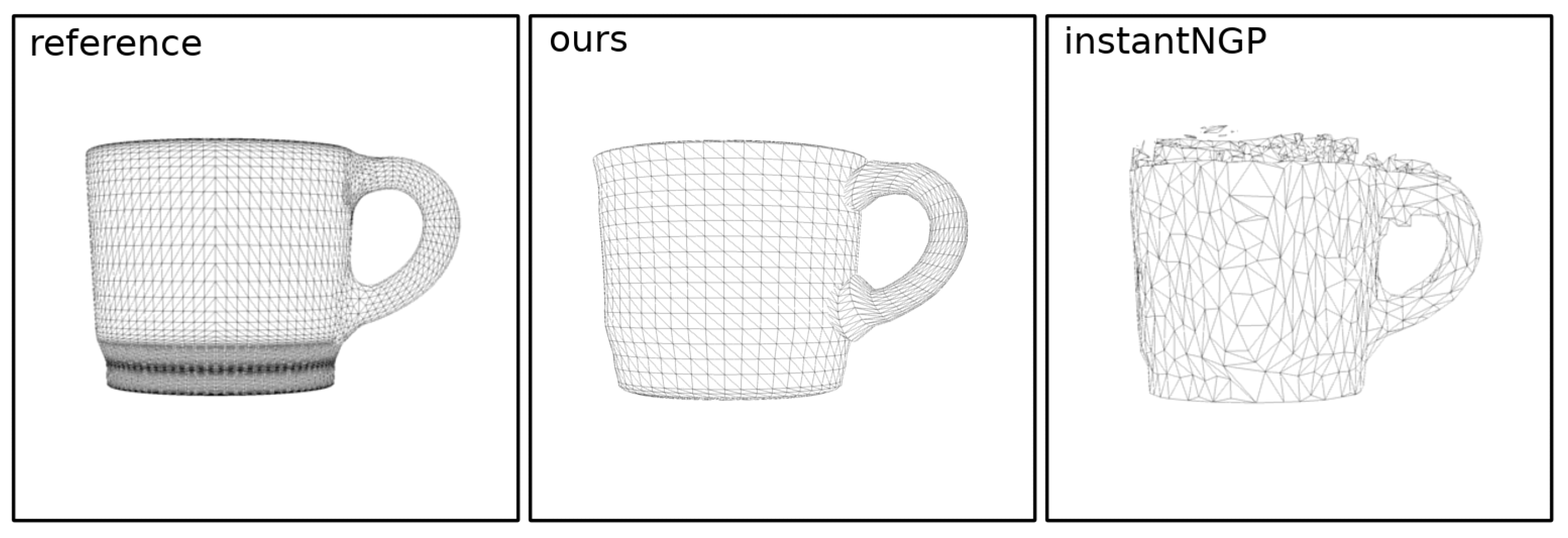
Figure 10 demonstrates the results of different algorithms on a relatively simple cup model. It shows that Pixel2Mesh failed to reconstruct the shape of the model from a single image, while methods that use multiple images achieved results comparable to ours. However, they both struggled to represent the concave shape of the model and produced meshes with significant artifacts. In Figure 11, some of the reconstructed meshes are visualized in wireframe mode. The diffSDF algorithm achieved a slightly better IoU value but took significantly more time. It also created a model with a rough surface, which will require refinement before use. The result of TGS is the closest to ours in terms of both IoU and required input data. However, the result of this method is a set of Gaussians, not a 3D mesh. The authors did not consider the problem of converting them into a mesh in [22] but, by analogy with NeRF-based methods, it can be assumed that such a conversion will reduce the quality of the result. The Gaussian representation makes it much more difficult to use or modify the resulting model because it is not supported by 3D modeling tools and rendering engines.

Figure 10. Results using our method compared to differentiable SDF reconstruction [30], InstantNGP [38], Pixel2Mesh [12], and TGS [22]. We measured the average silhouette intersection over union (IoU) between the reference and reconstructed models for 64 uniformly distributed viewpoints. Our approach is much better than Pixel2Mesh single-view reconstruction and produces results comparable to multi-view reconstruction methods.

Figure 11. Comparison of wireframe meshes. Our method is able to represent a model with fewer triangles and fewer tiny and deformed polygons, allowing it to be used directly in applications.

For more complex objects, such as trees and buildings, the ability to reconstruct the object’s structure becomes even more important. For most applications, such as, for example, video games, the reconstructed meshes need to be modified and augmented with some specific data. This becomes much easier if the initial mesh contains some structural information. In this particular case, it is necessary to distinguish between triangles related to different parts of a building or to leaves/branches of a tree in order to be able to meaningfully modify these models. Figure 12 shows the results of reconstruction of buildings and trees using different approaches.

Figure 12. The building and tree are reconstructed using our approach, differentiable SDF reconstruction [30], InstantNGP [38], Pixel2Mesh [12], and TGS [22]. InstantNGP failed to reconstruct the tree model and a mesh cannot be obtained from the radiance field it provided.

We also tested our approach on more models from the given classes and compared it with differentiable SDF reconstruction [30], InstantNGP [38], Pixel2Mesh [12], and TGS [22] algorithms. The diffSDF was tested with 2, 6, and 12 input images, and InstantNGP with 16 and 64 input images. The results of the comparison on the studied models are presented in Table 2. Although our method performs worse on average than the multi-view reconstruction algorithms diffSDF and InstantNGP in terms of the IoU metric, it is able to produce better models even if it fails to achieve high similarity to the reference images. This can be demonstrated using the tree models; the last two columns of the table and the bottom row in Figure 12 correspond to them. The IoU values for our approach are less than those for the diffSDF algorithm, and diffSDF produced a tree model that was closer in overall shape to the original, but failed to reconstruct the expected structure of the tree. So, our model is more suitable for many applications, especially considering that procedural models are easier to refine. Moreover, diffSDF does not create a triangle mesh but rather a 3D grid with values of reconstructed signed distance function. This representation of the scene imposes serious limitations, for example, it cannot be used with 2D texture maps.

Table 2. Average IoU (the larger the better) on different models. “–” is used in cases where the method failed to reconstruct a model that is even remotely similar to the reference mesh. See Section 4.2 for more details of algorithms used for comparison.

Algorithm	cup_1	cup_2	Building	tree_1	tree_2
diffSDF (2 views) [30]	0.787	0.422	0.728	0.665	0.746
diffSDF (6 views) [30]	0.960	0.502	0.967	0.876	0.911
diffSDF (12 views) [30]	0.984	0.669	0.979	0.900	0.941
InstantNGP (16 views) [38]	0.858	0.878	0.940	–	–
InstantNGP (64 views) [38]	0.905	0.930	0.971	–	–
pixel2Mesh (1 view) [12]	0.788	0.513	0.626	–	–
TGS (1 view) [22]	0.939	0.925	0.965	0.711	0.695
our approach (1 view)	0.948	0.972	0.886	0.509	0.573
our approach (2 views)	0.951	0.978	0.890	0.527	0.559
our approach (4 views)	0.962	0.979	0.869	0.571	0.613

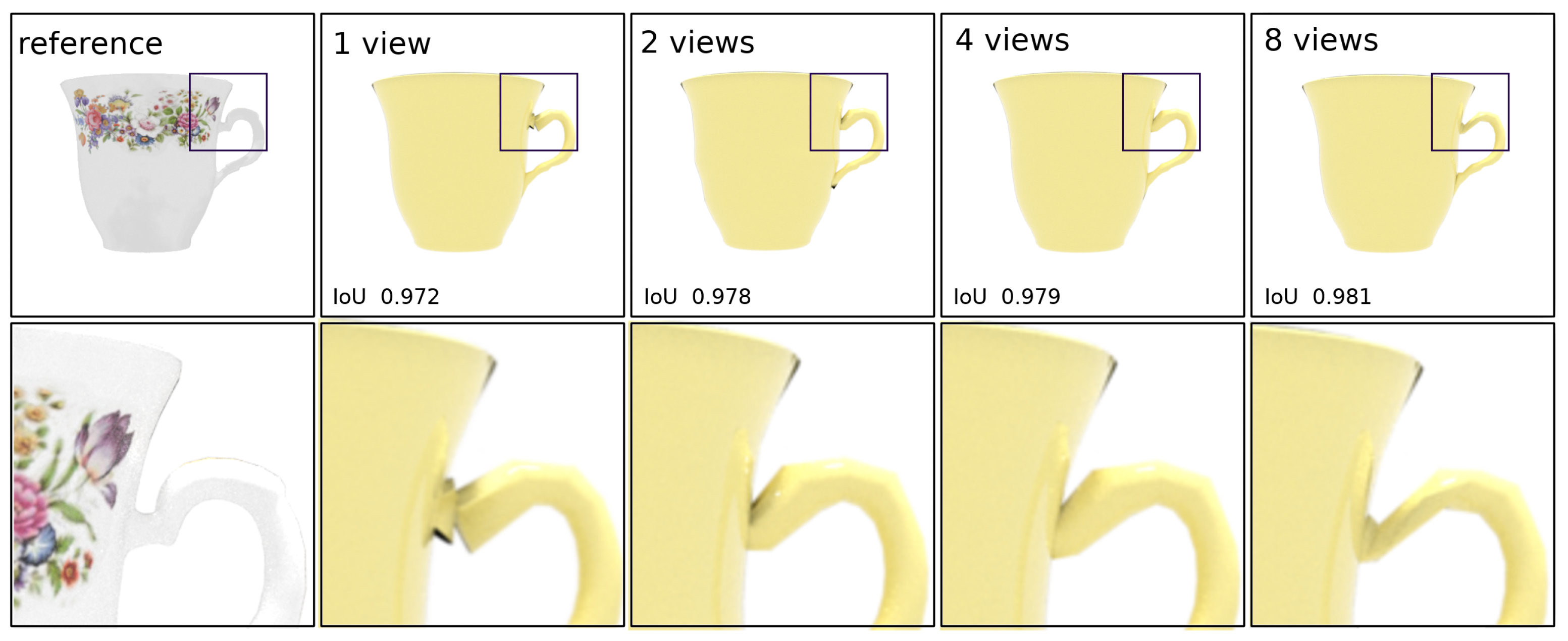
4.3. Multi-View Reconstruction

We mainly focused on single-view reconstruction in this work but our approach also supports multi-view reconstruction. However, although we have found that adding a new view does not usually result in a significant increase in quality, it can be useful for more complex objects or texture reconstruction. Figure 13 shows how increasing the number of views used for reconstruction affects the result for the relatively simple cap model. Although increasing the number of input images has almost no effect on quality, it significantly increases the running time of the algorithm, as shown in the Table 3.

Figure 13. Results of multi-view 3D reconstruction using our approach. A single viewpoint is sufficient for mesh reconstruction, and adding more viewpoints does not provide much improvement. However, a larger number of viewpoints allows for accurate texture reconstruction.

Table 3. Average IoU (the larger the better) and reconstruction time for cap model with our method using different numbers of input views.

Input Views	1 View	2 Views	4 Views	8 Views
IoU	0.972	0.978	0.979	0.981
time (min)	16.3	18.8	24.1	31.1

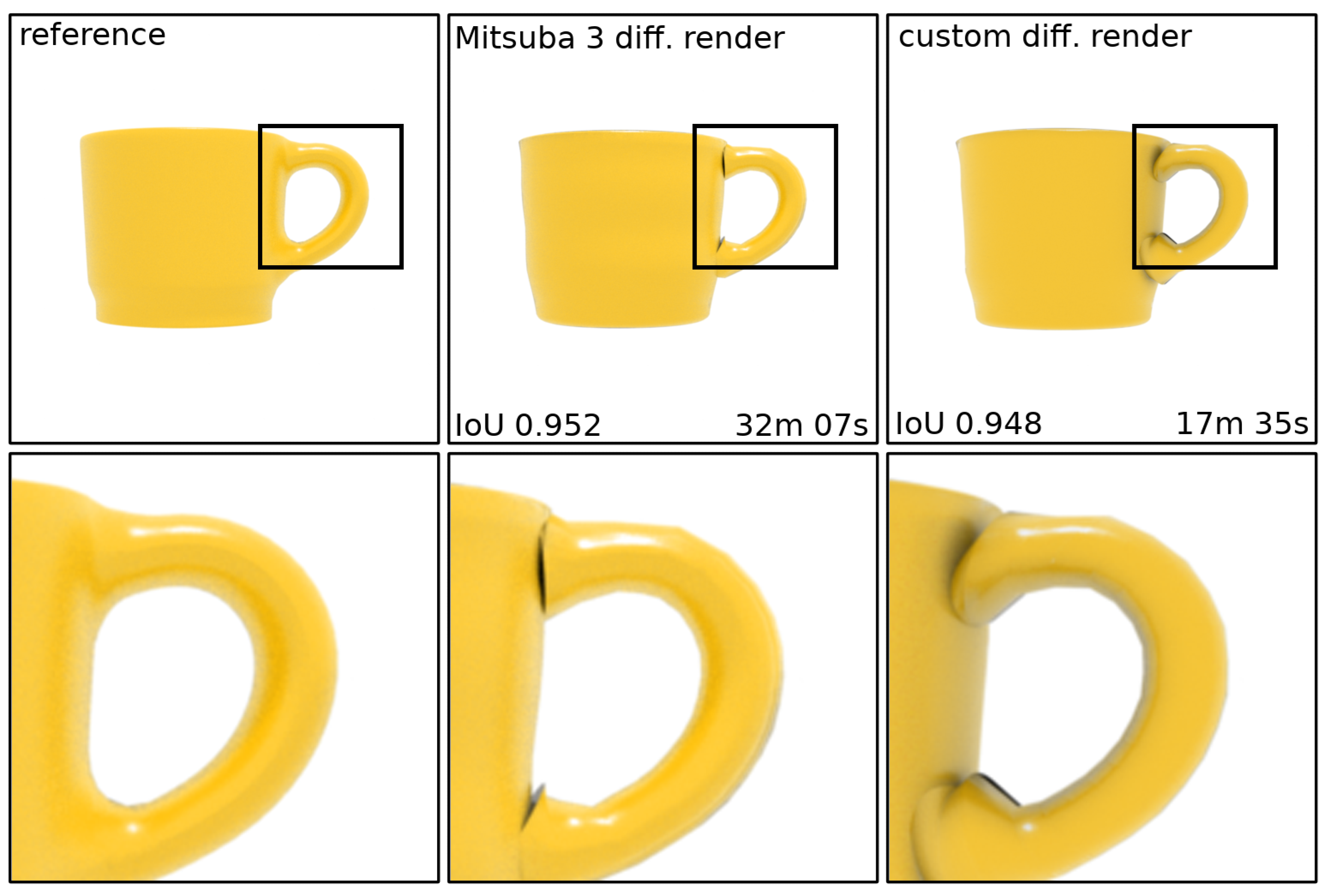
4.4. Differentiable Renderer

During the reconstruction process, most of the time is spent on differentiable rendering. The rendering is performed in silhouette mode, which means that we only obtain vertex position gradients from edge of the silhouette. This can be performed by Mitsuba 3 [60], but there is no need to use such a powerful tool for this simple task. Instead, we created our own implementation of a differentiable renderer that uses edge sampling [68] to calculate the required derivatives. Figure 14 shows that its use does not reduce the quality of reconstruction, but almost doubles its speed. Table 4 shows the difference in rendering speed for our renderer and Mitsuba 3.

Figure 14. Images: reference (left), reconstructed using Mitsuba 3 (center), and our own differentiable renderer (right).

Table 4. Differentiable rendering time (in ms) for the same mesh (about 3000 vertices) with different rendering resolutions using our differentiable render and Mitsuba [60].

Rendering Resolution	128 × 128	256 × 256	512 × 512
our differentiable render	6.7	23.2	87.1
Mitsuba 3	137.1	211.5	512.9

4.5. Discussion

Our work provides a bridge between two groups of methods: (1) inverse procedural modeling [44,45,46,47] and (2) approaches based on differential rendering [6,23,24,25,26]. Methods of the first group take 3D models as input, while methods of the second group calculate gradients from an input image for some conventional representation of a 3D model (mesh, SDF, etc.). Our approach allows us to directly obtain procedural generator parameters from the image. Unlike conventional meshes and SDF, procedural models are easy to edit and animate because a procedural model by its construction has separate parts with a specific semantic meaning. This allows our method to reconstruct 3D models that can later be modified and used by professional artists in existing software. This also opens up great opportunities for AI-driven 3D modeling tools such as text-to-3D or image-to-3D.

5. Conclusions

In this work, we present a novel approach to 3D reconstruction that estimates the input parameters of a procedural generator to reconstruct the model. In other words, we propose an image-driven approach for procedural modeling. We optimize the parameters of the procedural generator so that the rendering of the resulting 3D model is similar to the reference image or images. We have implemented several differentiable procedural generators and demonstrated that high-quality results can be achieved using them.

We also proposed an alternative version of the same approach that does not rely on the differentiability of the generator and allows it to achieve decent quality using already existing non-differentiable procedural generators. We have implemented an efficient strategy to find the optimal parameter sets for both versions of the proposed approach. For a small number of input images, our methods perform better than existing approaches and produce meshes with fewer artifacts.

Our approach works well with the certain class of objects that the underlying procedural generator can reproduce. The differentiable procedural generators used in this work are created from scratch and are limited in their capabilities. We consider that the main limitation of our method is that it is currently not capable of reconstructing arbitrary models. We also foresee challenges in scaling our approach to more complex procedural models with hundreds or thousands of parameters. Thus, the following topics for future work can be proposed:

• Development of a universal procedural generator with more flexible models, capable of representing a wide class of objects;
• Creation of a method for automated generation of the procedural generator itself, for example Large Language Models;
• Optimization or reconstruction of more complex models through increasing the number of parameters for optimization by an order of magnitude (this is a problem with genetic algorithms).

Overall, in future research we plan to extend our approach to a wider class of objects.

References

1. Xie, Y.; Takikawa, T.; Saito, S.; Litany, O.; Yan, S.; Khan, N.; Tombari, F.; Tompkin, J.; Sitzmann, V.; Sridhar, S. Neural fields in visual computing and beyond. Comput. Graph. Forum 2022, 41, 641–676. [Google Scholar] [CrossRef]
2. Pontes, J.K.; Kong, C.; Sridharan, S.; Lucey, S.; Eriksson, A.; Fookes, C. Image2mesh: A learning framework for single image 3d reconstruction. In Proceedings of the Computer Vision—ACCV 2018: 14th Asian Conference on Computer Vision, Perth, WA, Australia, 2–6 December 2018; pp. 365–381. [Google Scholar]
3. Yang, X.; Lin, G.; Zhou, L. ZeroMesh: Zero-shot Single-view 3D Mesh Reconstruction. arXiv 2022, arXiv:2208.02676. [Google Scholar]
4. Rakotosaona, M.J.; Manhardt, F.; Arroyo, D.M.; Niemeyer, M.; Kundu, A.; Tombari, F. NeRFMeshing: Distilling Neural Radiance Fields into Geometrically-Accurate 3D Meshes. arXiv 2023, arXiv:2303.09431. [Google Scholar] [CrossRef]
5. Tang, J.; Zhou, H.; Chen, X.; Hu, T.; Ding, E.; Wang, J.; Zeng, G. Delicate Textured Mesh Recovery from NeRF via Adaptive Surface Refinement. arXiv 2023, arXiv:2303.02091. [Google Scholar] [CrossRef]
6. Luan, F.; Zhao, S.; Bala, K.; Dong, Z. Unified Shape and SVBRDF Recovery using Differentiable Monte Carlo Rendering. Comput. Graph. Forum 2021, 40, 101–113. [Google Scholar] [CrossRef]
7. Park, J.J.; Florence, P.; Straub, J.; Newcombe, R.; Lovegrove, S. Deepsdf: Learning continuous signed distance functions for shape representation. In Proceedings of the IEEE/CVF Conference on Computer Vision and Pattern Recognition (CVPR), Long Beach, CA, USA, 16–20 June 2019; pp. 165–174. [Google Scholar]
8. Garifullin, A.; Shcherbakov, A.; Frolov, V. Fitting Parameters for Procedural Plant Generation. In Proceedings of the WSCG 2022: 30 International Conference in Central Europe on Computer Graphics, Visualization and Computer Vision, Pilsen, Czech Republic, 17–20 May 2022; pp. 282–288. [Google Scholar]
9. Garifullin, A.; Maiorov, N.; Frolov, V. Differentiable Procedural Models for Single-view 3D Mesh Reconstruction. In Proceedings of the Computer Graphics and Visual Computing (CGVC), Aberystwyth University, Wales, UK, 14–15 September 2023; pp. 39–43. [Google Scholar] [CrossRef]
10. Schonberger, J.L.; Frahm, J.M. Structure-from-motion revisited. In Proceedings of the IEEE Conference on Computer Vision and Pattern Recognition (CVPR), Las Vegas, NV, USA, 26 June–1 July 2016; pp. 4104–4113. [Google Scholar]
11. Cadena, C.; Carlone, L.; Carrillo, H.; Latif, Y.; Scaramuzza, D.; Neira, J.; Reid, I.; Leonard, J.J. Past, present, and future of simultaneous localization and mapping: Toward the robust-perception age. IEEE Trans. Robot. 2016, 32, 1309–1332. [Google Scholar] [CrossRef]
12. Wang, N.; Zhang, Y.; Li, Z.; Fu, Y.; Liu, W.; Jiang, Y.G. Pixel2mesh: Generating 3d mesh models from single rgb images. In Proceedings of the European Conference on Computer Vision (ECCV), Munich, Germany, 8–14 September 2018; pp. 52–67. [Google Scholar]
13. Nie, Y.; Han, X.; Guo, S.; Zheng, Y.; Chang, J.; Zhang, J.J. Total3dunderstanding: Joint layout, object pose and mesh reconstruction for indoor scenes from a single image. In Proceedings of the IEEE/CVF Conference on Computer Vision and Pattern Recognition (CVPR), Virtual, 14–19 June 2020; pp. 55–64. [Google Scholar]
14. Ye, Y.; Tulsiani, S.; Gupta, A. Shelf-supervised mesh prediction in the wild. In Proceedings of the IEEE/CVF Conference on Computer Vision and Pattern Recognition (CVPR), Virtual, 19–25 June 2021; pp. 8843–8852. [Google Scholar]
15. Choy, C.B.; Xu, D.; Gwak, J.; Chen, K.; Savarese, S. 3d-r2n2: A unified approach for single and multi-view 3d object reconstruction. In Proceedings of the Computer Vision–ECCV 2016: 14th European Conference, Amsterdam, The Netherlands, 11–14 October 2016; pp. 628–644. [Google Scholar]
16. Popov, S.; Bauszat, P.; Ferrari, V. Corenet: Coherent 3d scene reconstruction from a single rgb image. In Proceedings of the Computer Vision–ECCV 2020: 16th European Conference, Glasgow, UK, 23–28 August 2020; pp. 366–383. [Google Scholar]
17. Fan, H.; Su, H.; Guibas, L.J. A point set generation network for 3d object reconstruction from a single image. In Proceedings of the IEEE Conference on Computer Vision and Pattern Recognition (CVPR), Honolulu, HI, USA, 22–25 July 2017; pp. 605–613. [Google Scholar]
18. Chen, C.; Han, Z.; Liu, Y.S.; Zwicker, M. Unsupervised learning of fine structure generation for 3d point clouds by 2d projections matching. In Proceedings of the IEEE/CVF International Conference on Computer Vision (ICCV), Virtual, 11–19 October 2021; pp. 12466–12477. [Google Scholar]
19. Chen, W.; Ling, H.; Gao, J.; Smith, E.; Lehtinen, J.; Jacobson, A.; Fidler, S. Learning to predict 3d objects with an interpolation-based differentiable renderer. In Advances in Neural Information Processing Systems; Springer: Berlin, Germany, 2019; Volume 32. [Google Scholar]
20. Tatarchenko, M.; Richter, S.R.; Ranftl, R.; Li, Z.; Koltun, V.; Brox, T. What do single-view 3d reconstruction networks learn? In Proceedings of the IEEE/CVF Conference on Computer Vision and Pattern Recognition (CVPR), Long Beach, CA, USA, 16–20 June 2019; pp. 3405–3414. [Google Scholar]
21. Zhang, X.; Zhang, Z.; Zhang, C.; Tenenbaum, J.; Freeman, B.; Wu, J. Learning to reconstruct shapes from unseen classes. In Advances in Neural Information Processing Systems; Springer: Berlin, Germany, 2018; Volume 31. [Google Scholar]
22. Zou, Z.X.; Yu, Z.; Guo, Y.C.; Li, Y.; Liang, D.; Cao, Y.P.; Zhang, S.H. Triplane Meets Gaussian Splatting: Fast and Generalizable Single-View 3D Reconstruction with Transformers. arXiv 2023, arXiv:2312.09147. [Google Scholar]
23. Laine, S.; Hellsten, J.; Karras, T.; Seol, Y.; Lehtinen, J.; Aila, T. Modular primitives for high-performance differentiable rendering. ACM Trans. Graph. TOG 2020, 39, 194. [Google Scholar] [CrossRef]
24. Zhang, C.; Yu, Z.; Zhao, S. Path-space differentiable rendering of participating media. ACM Trans. Graph. TOG 2021, 40, 76. [Google Scholar] [CrossRef]
25. Deng, X.; Luan, F.; Walter, B.; Bala, K.; Marschner, S. Reconstructing translucent objects using differentiable rendering. In Proceedings of the ACM SIGGRAPH 2022 Conference, Vancouver, BC, Canada, 8–11 August 2022; pp. 38:1–38:10. [Google Scholar] [CrossRef]
26. Bangaru, S.P.; Gharbi, M.; Luan, F.; Li, T.M.; Sunkavalli, K.; Hasan, M.; Bi, S.; Xu, Z.; Bernstein, G.; Durand, F. Differentiable rendering of neural SDFs through reparameterization. In Proceedings of the SIGGRAPH Asia 2022 Conference, Daegu, Republic of Korea, 6–9 December 2022; pp. 22:1–22:9. [Google Scholar] [CrossRef]
27. Wickramasinghe, U.; Fua, P.; Knott, G. Deep Active Surface Models. In Proceedings of the IEEE/CVF Conference on Computer Vision and Pattern Recognition (CVPR), Virtual, 19–25 June 2021; pp. 11652–11661. [Google Scholar] [CrossRef]
28. Wang, Y.; Solomon, J. Fast quasi-harmonic weights for geometric data interpolation. ACM Trans. Graph. TOG 2021, 40, 73. [Google Scholar] [CrossRef]
29. Nicolet, B.; Jacobson, A.; Jakob, W. Large steps in inverse rendering of geometry. ACM Trans. Graph. TOG 2021, 40, 248. [Google Scholar] [CrossRef]
30. Vicini, D.; Speierer, S.; Jakob, W. Differentiable signed distance function rendering. ACM Trans. Graph. TOG 2022, 41, 125. [Google Scholar] [CrossRef]
31. Oswald, M.R. Convex Variational Methods for Single-View and Space-Time Multi-View Reconstruction. Ph.D. Thesis, Technische Universität München, Munich, Germany, 2015. Available online: https://mediatum.ub.tum.de/doc/1232437/928830.pdf (accessed on 11 November 2023).
32. Lombardi, S.; Simon, T.; Saragih, J.; Schwartz, G.; Lehrmann, A.; Sheikh, Y. Neural volumes: Learning dynamic renderable volumes from images. arXiv 2019, arXiv:1906.07751. [Google Scholar] [CrossRef]
33. Vicini, D.; Jakob, W.; Kaplanyan, A. A non-exponential transmittance model for volumetric scene representations. ACM Trans. Graph. TOG 2021, 40, 136. [Google Scholar] [CrossRef]
34. Yifan, W.; Serena, F.; Wu, S.; Öztireli, C.; Sorkine-Hornung, O. Differentiable surface splatting for point-based geometry processing. ACM Trans. Graph. TOG 2019, 38, 230. [Google Scholar] [CrossRef]
35. Rückert, D.; Franke, L.; Stamminger, M. ADOP: Approximate differentiable one-pixel point rendering. ACM Trans. Graph. TOG 2022, 41, 99. [Google Scholar] [CrossRef]
36. Mildenhall, B.; Srinivasan, P.P.; Tancik, M.; Barron, J.T.; Ramamoorthi, R.; Ng, R. Nerf: Representing scenes as neural radiance fields for view synthesis. Commun. ACM 2021, 65, 99–106. [Google Scholar] [CrossRef]
37. Fridovich-Keil, S.; Yu, A.; Tancik, M.; Chen, Q.; Recht, B.; Kanazawa, A. Plenoxels: Radiance fields without neural networks. In Proceedings of the IEEE/CVF Conference on Computer Vision and Pattern Recognition (CVPR), New Orleans, LA, USA, 19–24 June 2022; pp. 5501–5510. [Google Scholar]
38. Müller, T.; Evans, A.; Schied, C.; Keller, A. Instant neural graphics primitives with a multiresolution hash encoding. ACM Trans. Graph. TOG 2022, 41, 102. [Google Scholar] [CrossRef]
39. Hendrikx, M.; Meijer, S.; Van Der Velden, J.; Iosup, A. Procedural content generation for games: A survey. ACM Trans. Multimed. Comput. Commun. Appl. TOMM 2013, 9, 1. [Google Scholar] [CrossRef]
40. Freiknecht, J.; Effelsberg, W. A survey on the procedural generation of virtual worlds. Multimodal Technol. Interact. 2017, 1, 27. [Google Scholar] [CrossRef]
41. SpeedTree. 2017. Available online: http://www.speedtree.com (accessed on 11 November 2023).
42. Prusinkiewicz, P.; Lindenmayer, A. The Algorithmic Beauty of Plants; Springer: New York, NY, USA, 2012. [Google Scholar]
43. Yi, L.; Li, H.; Guo, J.; Deussen, O.; Zhang, X. Tree growth modelling constrained by growth equations. Comput. Graph. Forum 2018, 37, 239–253. [Google Scholar] [CrossRef]
44. Stava, O.; Pirk, S.; Kratt, J.; Chen, B.; Měch, R.; Deussen, O.; Benes, B. Inverse procedural modelling of trees. Comput. Graph. Forum 2014, 33, 118–131. [Google Scholar] [CrossRef]
45. Demir, I.; Aliaga, D.G.; Benes, B. Proceduralization for editing 3d architectural models. In Proceedings of the 2016 Fourth International Conference on 3D Vision (3DV), Stanford, CA, USA, 25–28 October 2016; pp. 194–202. [Google Scholar] [CrossRef]
46. Aliaga, D.G.; Demir, İ.; Benes, B.; Wand, M. Inverse procedural modeling of 3d models for virtual worlds. In Proceedings of the ACM SIGGRAPH 2016 Courses, Anaheim, CA, USA, 24–28 July 2018; pp. 1–316. [Google Scholar] [CrossRef]
47. Guo, J.; Jiang, H.; Benes, B.; Deussen, O.; Zhang, X.; Lischinski, D.; Huang, H. Inverse procedural modeling of branching structures by inferring L-systems. ACM Trans. Graph. TOG 2020, 39, 155. [Google Scholar] [CrossRef]
48. Hu, Y.; He, C.; Deschaintre, V.; Dorsey, J.; Rushmeier, H. An inverse procedural modeling pipeline for SVBRDF maps. ACM Trans. Graph. TOG 2022, 41, 18. [Google Scholar] [CrossRef]
49. Wu, F.; Yan, D.M.; Dong, W.; Zhang, X.; Wonka, P. Inverse procedural modeling of facade layouts. arXiv 2013, arXiv:1308.0419. [Google Scholar] [CrossRef]
50. Zhao, S.; Luan, F.; Bala, K. Fitting procedural yarn models for realistic cloth rendering. ACM Trans. Graph. TOG 2016, 35, 51. [Google Scholar] [CrossRef]
51. Trunz, E.; Klein, J.; Müller, J.; Bode, L.; Sarlette, R.; Weinmann, M.; Klein, R. Neural inverse procedural modeling of knitting yarns from images. arXiv 2023, arXiv:2303.00154. [Google Scholar] [CrossRef]
52. Gaillard, M.; Krs, V.; Gori, G.; Měch, R.; Benes, B. Automatic differentiable procedural modeling. Comput. Graph. Forum 2022, 41, 289–307. [Google Scholar] [CrossRef]
53. Zeng, J.; Zhang, Y.; Zhan, S.; Liu, C. Reconstructing symmetric curved surfaces from a single image and its application. In Proceedings of the Interactive Technologies and Sociotechnical Systems: 12th International Conference, VSMM 2006, Xi’an, China, 18–20 October 2006; pp. 204–213. [Google Scholar] [CrossRef]
54. Hosseini, S.M.H.; Nasiri, S.M.; Hosseini, R.; Moradi, H. Single-View 3d Reconstruction of Surface of Revolution. SSRN 2022, 12, 4117409. [Google Scholar] [CrossRef]
55. Pang, H.E.; Biljecki, F. 3D building reconstruction from single street view images using deep learning. Int. J. Appl. Earth Obs. Geoinf. 2022, 112, 102859. [Google Scholar] [CrossRef]
56. Venkat, A.; Jinka, S.S.; Sharma, A. Deep textured 3d reconstruction of human bodies. arXiv 2018, arXiv:1809.06547. [Google Scholar] [CrossRef]
57. Huang, Z.; Khan, R. A review of 3D human body pose estimation and mesh recovery. Digit. Signal Process. 2022, 128, 103628. [Google Scholar] [CrossRef]
58. Kerbl, B.; Kopanas, G.; Leimkühler, T.; Drettakis, G. 3D Gaussian Splatting for Real-Time Radiance Field Rendering. ACM Trans. Graph. 2023, 42, 1317–1330. [Google Scholar] [CrossRef]
59. Rakotosaona, M.J.; Manhardt, F.; Arroyo, D.M.; Niemeyer, M.; Kundu, A.; Tombari, F. NeRFMeshing: Distilling Neural Radiance Fields into Geometrically-Accurate 3D Meshes. In Proceedings of the International Conference on 3D Vision (3DV), Prague, Czech Republic, 12–15 September 2023. [Google Scholar]
60. Wenzel, J.; Speierer, S.; Roussel, N.; Nimier-David, M.; Vicini, D.; Zeltner, T.; Nicolet, B.; Crespo, M.; Leroy, V.; Zhang, Z. Mitsuba 3 Renderer. 2022. Available online: https://mitsuba-renderer.org (accessed on 11 November 2023).
61. Bell, B.M. CppAD: A package for C++ algorithmic differentiation. Comput. Infrastruct. Oper. Res. 2012, 57, 10. [Google Scholar]
62. Mitchell, M. An Introduction to Genetic Algorithms; MIT Press: Cambridge, MA, USA, 1998. [Google Scholar]
63. Neri, F.; Cotta, C. Memetic algorithms and memetic computing optimization: A literature review. Swarm Evol. Comput. 2012, 2, 1–14. [Google Scholar] [CrossRef]
64. Hädrich, T.; Benes, B.; Deussen, O.; Pirk, S. Interactive modeling and authoring of climbing plants. Comput. Graph. Forum 2017, 36, 49–61. [Google Scholar] [CrossRef]
65. Yi, L.; Li, H.; Guo, J.; Deussen, O.; Zhang, X. Light-Guided Tree Modeling of Diverse Biomorphs. In Proceedings of the 23rd Pacific Conference on Computer Graphics and Applications “Pacific Graphics 2015”, Beijing, China, 7–9 October 2015; pp. 53–57. [Google Scholar] [CrossRef]
66. Weber, J.; Penn, J. Creation and rendering of realistic trees. In Proceedings of the 22nd Annual Conference on Computer Graphics and Interactive Techniques, Los Angeles, CA, USA, 6–11 August 1995; pp. 119–128. [Google Scholar]
67. Li, B.; Kałużny, J.; Klein, J.; Michels, D.L.; Pałubicki, W.; Benes, B.; Pirk, S. Learning to reconstruct botanical trees from single images. ACM Trans. Graph. TOG 2021, 40, 231. [Google Scholar] [CrossRef]
68. Li, T.M.; Aittala, M.; Durand, F.; Lehtinen, J. Differentiable monte carlo ray tracing through edge sampling. ACM Trans. Graph. TOG 2018, 37, 222. [Google Scholar] [CrossRef]
Disclaimer/Publisher’s Note: The statements, opinions and data contained in all publications are solely those of the individual author(s) and contributor(s) and not of MDPI and/or the editor(s). MDPI and/or the editor(s) disclaim responsibility for any injury to people or property resulting from any ideas, methods, instructions or products referred to in the content.
Article Metrics
Citations
Article Access Statistics
Multiple requests from the same IP address are counted as one view.