Medical and Engineering Applications for Estimation and Prediction of a New Competing Risks Model: A Bayesian Approach

Abstract

The Bayesian approach offers a flexible, interpretable and powerful framework for statistical analysis, making it a valuable tool to help in making optimal decisions under uncertainty. It incorporates prior knowledge or beliefs about the parameters, which can lead to more accurate and informative results. Also, it offers credible intervals as a measure of uncertainty, which are often more interpretable than confidence intervals. Hence, the Bayesian approach is utilized to estimate the parameters, reliability function, hazard rate function and reversed hazard rate function of a new competing risks model. A squared error loss function as a symmetric loss function and a linear exponential loss function as an asymmetric loss function are employed to derive the Bayesian estimators. Credible intervals of the parameters, reliability function, hazard rate function and reversed hazard rate function are obtained. Predicting future observations is important in many fields, from finance and weather forecasting to healthcare and engineering. Thus, two-sample prediction (as a special case of the multi-sample prediction) for future observation is considered. An adaptive Metropolis algorithm is applied to conduct a simulation study to evaluate the performance of the Bayes estimates and predictors. Moreover, two applications of medical and engineering data sets are used to test and validate the theoretical results, ensuring that they are accurate, applicable to real-world scenarios and contribute to the understanding of the world and inform decision-making.

1. Introduction

Competing risks often occur in reliability studies and demographic, medical, biological sciences and engineering applications, where there is more than one cause or mode of failure. These failure modes in some sense compete to cause the failure of the experimental item. So, in statistical literature this is known as competing risks. Also, competing risks happened in series systems, in which their components are arranged in series. The lifetime of each component has a certain distribution with certain parameters. By assuming that the lifetimes of the components of the series system are statistically independent of each other, the lifetime of the series system can be obtained as the minimum of its components lifetimes. Additionally, the competing risks model is also known as a series model, additive model and multi-risk model.

Based on the concept of competing risks, a wide range of lifetime distributions have been introduced in the statistical literature, each contributing to the understanding and modeling of time-to-event data. Key contributions in this area include foundational work by [1] and subsequent developments by [2,3,4,5,6,7,8,9,10,11,12,13,14,15,16,17,18,19,20]. More recently, [21] proposed the additive xgamma-Burr XII distribution, introducing further flexibility to the modeling framework by accommodating complex hazard behaviors.

Incorporating competing risks into structural reliability assessments has been further refined by recent methodologies, such as power transformation approaches that improve access to reliability indexes under structural uncertainties (see [22]). Similarly, in seismic fragility analysis, particularly for nuclear power plants, structural parameter uncertainty introduces additional competing risk factors that influence fragility estimation (see [23]).

The additive xgamma-BurrXII (Xg-BXII) distribution was introduced by [21] by considering a series system with two components functioning independently in series. The lifetime of the first component, $X_1$, has the xgamma (Xg) distribution with parameters $\alpha$, and the lifetime of the second component, $X_2$, has Burr XII (BXII) distribution with parameters $c$ and $k$. Therefore, the lifetime of the system $X=\min \left\{X_1,X_2\right\}$ has the Xg-BXII distribution with a vector of parameters $\underset{\_}{\psi }=\left(\alpha ,c,k\right)$. The probability density function (pdf), cumulative distribution function (cdf), reliability function (rf), hazard rate function (hrf) and reversed hazard rate function (rhrf) of the Xg-BXII distribution are expressed, respectively, as follows:

$$\begin{array}{c}f\left(x;\underset{\_}{\psi }\right)=\left[{\alpha }^2\left(1+{\displaystyle \frac{\alpha x^2}{2}}\right)+{\displaystyle \frac{ck{x}^{c-1}\left(1+\alpha +\alpha x+\frac{{\alpha }^2{x}^2}{2}\right)}{\left(1+x^c\right)}}\right]{\displaystyle \frac{{\left(1+x^c\right)}^{-k}{e}^{-\alpha x}}{1+\alpha }},\\ x>0;\underset{\_}{\psi }>\underset{\_}{0},\end{array}$$

(1)

$$F\left(x;\underset{\_}{\psi }\right)=1-{\displaystyle \frac{1+\alpha +\alpha x+\frac{{\alpha }^2{x}^2}{2}}{\left(1+\alpha \right){\left(1+x^c\right)}^k}}{e}^{-\alpha x},\hspace{1em}\hspace{1em}\hspace{1em}x>0; \underset{\_}{\psi }>\underset{\_}{0},$$

(2)

$$R\left(x;\underset{\_}{\psi }\right)={\displaystyle \frac{1+\alpha +\alpha x+\frac{{\alpha }^2{x}^2}{2}}{\left(1+\alpha \right){\left(1+x^c\right)}^k}}{e}^{-\alpha x},\hspace{1em}\hspace{1em}x>0; \underset{\_}{\psi }>\underset{\_}{0},$$

(3)

$$h\left(x;\underset{\_}{\psi }\right)={\displaystyle \frac{{\alpha }^2\left(1+\frac{\alpha x^2}{2}\right)}{1+\alpha +\alpha x+\frac{{\alpha }^2{x}^2}{2}}}+{\displaystyle \frac{ck{x}^{c-1}}{1+x^c}},\hspace{1em}\hspace{1em}x>0; \underset{\_}{\psi }>\underset{\_}{0},$$

(4)

and

$$r\left(x;\underset{\_}{\psi }\right)={\displaystyle \frac{\left[{\alpha }^2\left(1+\frac{\alpha x^2}{2}\right)+\frac{ck{x}^{c-1}\left(1+\alpha +\alpha x+\frac{{\alpha }^2{x}^2}{2}\right)}{1+x^c}\right]}{\left(1+\alpha \right){\left(1+x^c\right)}^k{e}^{\alpha x}-\left(1+\alpha +\alpha x+\frac{{\alpha }^2{x}^2}{2}\right)}},\hspace{1em}\hspace{1em}x>0; \underset{\_}{\psi }>\underset{\_}{0},$$

(5)

where

$$\underset{\_}{\psi }=\left(\alpha ,c,k\right).$$

(6)

The importance of this distribution seems to be from its pdf and hrf, which display high flexibility and diversity in shape (see, e.g., [24]). The Xg-BXII distribution hrf has two main shapes, bathtub and modified bathtub, which are very important in reliability analyses. These shapes increase the applicability of this distribution for lifetime data modeling. Moreover, the Xg-BXII distribution has some new additive models as special cases, some of which are well-known models. Ref. [21] derived some main properties of the Xg-BXII distribution and estimated the model parameters, the rf, hrf and rhrf, using the maximum likelihood method. Also, they obtained the asymptotic confidence intervals of the parameters rf, hrf and rhrf. Moreover, they demonstrated the applicability and flexibility of the Xg-BXII distribution over some existing distributions through four applications.

This article focuses on Bayesian estimation of the parameters of the Xg-BXII distribution and its rf, hrf and rhrf due to its advantages. Among these advantages is that it considers the prior information about the unknown parameters represented in the joint prior distribution and the sample information represented in the likelihood function (LF) and combines them in the posterior distribution (see, e.g., [25]). Another advantage of the Bayesian estimation is that it is widely appropriate in the cases of small sample sizes and censored data. On the other hand, the most popular loss functions in Bayesian estimation problems are the squared error (SE) loss function as a symmetric loss function and the linear exponential (LINEX) loss function, which was introduced by [26] and popularized by [27] as an asymmetric loss function. The SE and LINEX loss functions are defined, respectively, as

$$L_1\left(\psi ,\tilde{\psi }\right)=d{\left(\psi -\tilde{\psi }\right)}^2,$$

(7)

and

$$L_2\left(\psi ,\tilde{\psi }\right)\propto e^{\nu \mathsf{\Delta }}-\nu \mathsf{\Delta }-1, \nu \ne 0,$$

(8)

where $\psi$ is an unknown parameter and $\tilde{\psi }$ is its Bayes estimator, $d$ is a constant, $\nu$ is a constant that determines the shape of the loss function and $\mathsf{\Delta }=\tilde{\psi }-\psi$.

The prediction of future observations is an important problem in many practical applications, such as agricultural, industrial, demographic, medical, biological and engineering experiments. Therefore, in this article, the problem of predicting a future observation from the Xg-BXII distribution based on one-sample and two-sample prediction approaches is considered.

Many researchers have considered predictions for future observation from different lifetime distributions. Ref. [28] applied Bayesian one-sample and two-sample prediction to predict a future observation using a Type II censored sample from a general class of distributions. Ref. [29] studied one-sample and two-sample Bayesian prediction for future observation from Type II censored samples from the flexible Weibull extension distribution. Ref. [30] discussed the Bayesian prediction for the Nadarajah–Haghighi distribution under progressive Type II censored samples for one-sample and two-sample prediction schemes. Ref. [31] studied the one-sample and two-sample prediction schemes for a future observation from Burr X distribution based on a unified hybrid censoring scheme using likelihood and Bayesian prediction methods. Recently, ref. [32] derived Bayesian prediction intervals for future observations based on unified hybrid censored data from the three-parameter BXII distribution using both one-sample and two-sample prediction techniques. More recently, ref. [33] presented one-sample and two-sample non-Bayesian and Bayesian prediction of future observations from the additive flexible Weibull extension–Lomax distribution based on Type II censored samples. Ref. [34] discussed one-sample and two-sample prediction problems based on observed Type II progressive censored samples and predictive intervals under a Bayesian framework.

The rest of this paper is organized as follows: in Section 2, Bayesian estimation for the unknown parameters rf, hrf and rhrf of the Xg-BXII distribution are derived under the SE and LINEX loss functions. Also, credible intervals (CIs) are obtained. A Bayesian two-sample prediction of future observation from the Xg-BXII distribution is discussed in Section 3. Additionally, in Section 4, a simulation study is presented to illustrate the theoretical results derived for Bayesian estimation and prediction by applying the adaptive Metropolis (AM) algorithm. Moreover, applications are given in Section 5 to show the applicability of the derived estimators and predictors. Finally, a general conclusion is given in Section 6.

2. Bayesian Estimation

In this section, Bayes estimators of the parameters rf, hrf and rhrf of the Xg-BXII distribution under the SE and LINEX loss functions are given. Also, CIs are obtained.

Suppose that $x_1, x_2,\dots , x_n$ is a random sample of size $n$ from the Xg-BXII distribution with parameter vector $\underset{\_}{\psi }=\left(\alpha ,c,k\right)$. Then, the LF is given by

$$\begin{array}{c}L\left(\underset{\_}{\psi }|\underset{\_}{x}\right)=n!\left[{\displaystyle \prod _{i=1}^n}f\left(x_{\left(i\right)};\underset{\_}{\psi }\right)\right]\hfill \\ ={\displaystyle \frac{n!}{{\left(1+\alpha \right)}^n}}{e}^{-\alpha \sum _{i=1}^n{x}_{\left(i\right)}}{\displaystyle \prod _{i=1}^n}\left[{\alpha }^2\left(1+{\displaystyle \frac{\alpha x_{\left(i\right)}^2}{2}}\right)+{\displaystyle \frac{ck{x}_{\left(i\right)}^{c-1}{u}_{\left(i\right)}}{w_{\left(i\right)}}}\right]{\displaystyle \prod _{i=1}^n}{w}_{\left(i\right)}^{-k}, \end{array}$$

(9)

where

$$u_{\left(i\right)}=1+\alpha +\alpha x_{\left(i\right)}+{\displaystyle \frac{{\alpha }^2{x}_{\left(i\right)}^2}{2}},$$

(10)

and

$$w_{\left(i\right)}=1+x_{\left(i\right)}^c.$$

(11)

Treating the parameters $\underset{\_}{\psi }=\left(\alpha ,c,k\right)=\left({\psi }_1,{\psi }_2,{\psi }_3\right)$ of the Xg-BXII distribution as unknown random variables, each one is assigned an independent gamma prior distribution, which is defined by the pdf:

$${\pi }_j\left({\psi }_j\right)\propto {\psi }_j^{a_j-1}{e}^{-b_j{\psi }_j},\hspace{1em}\hspace{1em}\hspace{1em}{\psi }_j>0; a_j, b_j>0, j=1,2,3,$$

(12)

where $a_j$ and $b_j$ are the hyperparameters of the parameters ${\psi }_j$ for $j=1,2,3$.

Therefore, the joint prior distribution of $\underset{\_}{\psi }$ is given by

$$\begin{array}{cc}\hfill \pi \left(\underset{\_}{\psi }\right)& \propto {\displaystyle \prod _{j=1}^3}{\pi }_j\left({\psi }_j\right)\propto {\displaystyle \prod _{j=1}^3}{\psi }_j^{a_j-1}{e}^{-b_j{\psi }_j}\hfill \\ & \propto {\alpha }^{a_1-1}{c}^{a_2-1}{k}^{a_3-1} e^{-\left(\alpha b_1+c{b}_2+k{b}_3\right)}, {\psi }_j>0; a_j, b_j>0, j=1,2,3,\hfill \end{array}$$

(13)

where $a_j$ and $b_j$ are the hyperparameters ${\psi }_j$ of the joint prior distribution for $j=1,2,3$.

Hence, the joint posterior distribution of $\underset{\_}{\psi }=\left(\alpha ,c,k\right)=\left({\psi }_1,{\psi }_2,{\psi }_3\right)$ can be obtained using $\left(9\right)$ and $\left(13\right)$ as follows:

$$\pi \left(\underset{\_}{\psi }|\underset{\_}{x}\right)=AL\left(\underset{\_}{\psi }|\underset{\_}{x}\right)\pi \left(\underset{\_}{\psi }\right).$$

Then,

$$\begin{array}{c}\pi \left(\underset{\_}{\psi }|\underset{\_}{x}\right)=\mathrm{A}{\displaystyle \frac{{\alpha }^{a_1-1}{c}^{a_2-1}{k}^{a_3-1}}{{\left(1+\alpha \right)}^n}}{e}^{-\left[\alpha \left(\sum _{i=1}^n{x}_{\left(i\right)}+b_1\right)+c{b}_2+k{b}_3\right]}\\ \hspace{1em}\hspace{1em}\hspace{1em}\hspace{1em}\hspace{1em}\times {\displaystyle \prod _{i=1}^n}\left[{\alpha }^2\left(1+{\displaystyle \frac{\alpha x_{\left(i\right)}^2}{2}}\right)+{\displaystyle \frac{ck{x}_{\left(i\right)}^{c-1}{u}_{\left(i\right)}}{w_{\left(i\right)}}}\right]{\displaystyle \prod _{i=1}^n}{w}_{\left(i\right)}^{-k},\end{array}$$

(14)

where $\mathrm{A}$ is the normalized constant defined by

$$\begin{array}{c}{\mathrm{A}}^{-1}={\int }_{\underset{\_}{\psi }}{\displaystyle \frac{{\alpha }^{a_1-1}{c}^{a_2-1}{k}^{a_3-1}}{{\left(1+\alpha \right)}^n}}{e}^{-\left[\alpha \left(\sum _{i=1}^n{x}_{\left(i\right)}+b_1\right)+c{b}_2+k{b}_3\right]}\\ \hspace{1em}\hspace{1em}\times {\displaystyle \prod _{i=1}^n}\left[{\alpha }^2\left(1+{\displaystyle \frac{\alpha x_{\left(i\right)}^2}{2}}\right)+{\displaystyle \frac{ck{x}_{\left(i\right)}^{c-1}{u}_{\left(i\right)}}{w_{\left(i\right)}}}\right]{\displaystyle \prod _{i=1}^n}{w}_{\left(i\right)}^{-k}d\underset{\_}{\psi },\end{array}$$

(15)

where

$${\int }_{\underset{\_}{\psi }}={\int }_{\alpha =0}^{\mathrm{\infty }}{\int }_{c=0}^{\mathrm{\infty }}{\int }_{k=0}^{\mathrm{\infty }}\hspace{1em}\mathrm{a}\mathrm{n}\mathrm{d}\hspace{1em}d\underset{\_}{\psi }=d\alpha dcdk.$$

(16)

The marginal posterior distribution of the parameter ${\psi }_j$ can be obtained as

$${\pi }_j\left({\psi }_j|\underset{\_}{x}\right)=\underset{{\underset{\_}{\psi }}_l}{\int }\pi \left(\underset{\_}{\psi }|\underset{\_}{x}\right)d{\underset{\_}{\psi }}_l,\hspace{1em}l\ne j,\hspace{1em}l,j=1,2,3.$$

(17)

Gamma priors were selected due to their flexibility and their compatibility with the parameters under consideration, which are positive and therefore align well with the support of the gamma distribution. The gamma prior also allows to incorporate prior knowledge about the scale of the parameters in a straightforward manner, using the shape and rate parameters to encode beliefs about their likely values. The gamma distribution enables us to control the degree of informativeness of the prior by adjusting these parameters.

2.1. Point Estimation

This subsection is devoted to derive point Bayes estimators of the parameters rf, hrf and rhrf of the Xg-BXII distribution under two loss functions: the SE and the LINEX loss functions.

I.

Bayesian estimation under the squared error loss function

Under the SE loss function, the Bayes estimator of a parameter $\psi$, denoted by ${\tilde{\psi }}_{SE}$, is an estimator that minimizes the expected loss function, which is known as the posterior risk (PR) and is defined as

$$\begin{array}{c}PR\left({\tilde{\psi }}_{SE}\right)=E\left[L_1\left(\psi ,\tilde{\psi }\right)\right]=\underset{\psi }{\int }{L}_1\left(\psi ,\tilde{\psi }\right){\pi }^{*}\left(\psi |\underset{\_}{x}\right)d\psi =E\left({\psi }^2|\underset{\_}{x}\right)-{\left[E\left(\psi |\underset{\_}{x}\right)\right]}^2\\ \hspace{1em}\hspace{1em}\hspace{1em}\hspace{1em}\hspace{1em}\hspace{1em}=V\left(\psi |\underset{\_}{x}\right).\hfill \end{array}$$

(18)

(For more details see [35,36]).

The Bayes estimator of $\psi$ that minimizes Equation $\left(18\right)$ is given by

$${\tilde{\psi }}_{SE}=E\left(\psi |\underset{\_}{x}\right).$$

(19)

Therefore, Bayes estimators of the parameters $\underset{\_}{\psi }=\left({\psi }_1,{\psi }_2,{\psi }_3\right)$ are the means of their marginal posterior distributions. Hence, based on the marginal posterior distribution in $\left(17\right)$, the Bayes estimators can be obtained as follows:

$$\begin{array}{c}{\tilde{\psi }}_{jSE}=E\left({\psi }_j|\underset{\_}{x}\right)=\underset{{\psi }_j}{\int }{\psi }_j{\pi }_j\left({\psi }_j|\underset{\_}{x}\right)d{\psi }_j=\underset{\underset{\_}{\psi }}{\int }{\psi }_j\pi \left(\underset{\_}{\psi }|\underset{\_}{x}\right)d\underset{\_}{\psi }\hfill \\ \hspace{1em}={\int }_{\underset{\_}{\psi }}{\psi }_j\mathrm{A}{\displaystyle \frac{{\alpha }^{a_1-1}{c}^{a_2-1}{k}^{a_3-1}}{{\left(1+\alpha \right)}^n}}{e}^{-\left[\alpha \left(\sum _{i=1}^n{x}_{\left(i\right)}+b_1\right)+c{b}_2+k{b}_3\right]}\times {\displaystyle \prod _{i=1}^n}\left[{\alpha }^2\left(1+{\displaystyle \frac{\alpha x_{\left(i\right)}^2}{2}}\right)+{\displaystyle \frac{ck{x}_{\left(i\right)}^{c-1}{u}_{\left(i\right)}}{w_{\left(i\right)}}}\right]{\displaystyle \prod _{i=1}^n}{w}_{\left(i\right)}^{-k}d\underset{\_}{\psi },\hfill \\ \hfill j=1,2,3,\end{array}$$

(20)

where $\underset{\_}{\psi }$, $\mathrm{A}$, $u_{\left(i\right)}, w_{\left(i\right)}$, ${\int }_{\underset{\_}{\psi }}$ and $d\underset{\_}{\psi }$ are defined earlier in this section, as $\underset{\_}{\psi }$ is defined in $\left(6\right)$, $\mathrm{A}$ is the normalized constant defined in $\left(15\right)$, $u_{\left(i\right)}$ and $w_{\left(i\right)}$ are given, respectively, in $\left(10\right)$ and $\left(11\right)$ and ${\int }_{\underset{\_}{\psi }}$ and $d\underset{\_}{\psi }$ are given in $\left(16\right)$.

Also, the Bayes estimators of the rf, hrf and rhrf can be obtained using $\left(3\right)–\left(5\right)$ and $\left(14\right)$ as follows:

$$\begin{array}{c}{\tilde{R}}_{SE}\left(x_0\right)=E\left[R\left(x_0\right)\left|\underset{\_}{x}\right.\right]={\int }_{\underset{\_}{\psi }}R\left(x_0\right)\pi \left(\underset{\_}{\psi }|\underset{\_}{x}\right)d\underset{\_}{\psi }\hfill \\ \hspace{1em}\hspace{1em}={\int }_{\underset{\_}{\psi }}\mathrm{A}{\displaystyle \frac{{\alpha }^{a_1-1}{c}^{a_2-1}{k}^{a_3-1}{u}_{\left(0\right)}}{{\left(1+\alpha \right)}^{n+1}{w}_{\left(0\right)}^{-k}}}{e}^{-\left[\alpha \left(\sum _{i=1}^n{x}_{\left(i\right)}+x_0+b_1\right)+c{b}_2+k{b}_3\right]}\\ \times {\displaystyle \prod _{i=1}^n}\left[{\alpha }^2\right(1+{\displaystyle \frac{\alpha x_{\left(i\right)}^2}{2}})+\frac{ck{x}_{\left(i\right)}^{c-1}{u}_{\left(i\right)}}{w_{\left(i\right)}}]{\displaystyle \prod _{i=1}^n}{w}_{\left(i\right)}^{-k}d\underset{\_}{\psi },\end{array}$$

(21)

where

$$u_{\left(0\right)}=1+\alpha +\alpha x_0+{\displaystyle \frac{{\alpha }^2{x}_0^2}{2}},$$

(22)

and

$$w_{\left(0\right)}=1+x_0^c.$$

(23)

$$\begin{array}{c}{\tilde{h}}_{SE}\left(x_0\right)=E\left[h\left(x_0\right)\left|\underset{\_}{x}\right.\right]={\int }_{\underset{\_}{\psi }}h\left(x_0\right)\pi \left(\underset{\_}{\psi }|\underset{\_}{x}\right)d\underset{\_}{\psi }\hfill \\ ={\int }_{\underset{\_}{\psi }}\mathrm{A}{\displaystyle \frac{{\alpha }^{a_1+1}{c}^{a_2-1}{k}^{a_3-1}}{{\left(1+\alpha \right)}^n}}{e}^{-\left[\alpha \left(\sum _{i=1}^n{x}_{\left(i\right)}+b_1\right)+c{b}_2+k{b}_3\right]}\left[{\displaystyle \frac{\left(1+\frac{\alpha x_0^2}{2}\right)}{u_{\left(0\right)}}}+{\displaystyle \frac{ck{x}^{c-1}}{w_{\left(0\right)}}}\right]\\ \times {\displaystyle \prod _{i=1}^n}\left[{\alpha }^2\left(1+{\displaystyle \frac{\alpha x_{\left(i\right)}^2}{2}}\right)+{\displaystyle \frac{ck{x}_{\left(i\right)}^{c-1}{u}_{\left(i\right)}}{w_{\left(i\right)}}}\right]{\displaystyle \prod _{i=1}^n}{w}_{\left(i\right)}^{-k}d\underset{\_}{\psi },\end{array}$$

(24)

and

$$\begin{array}{c}{\tilde{r}}_{SE}\left(x_0\right)=E\left[r\left(x_0\right)\left|\underset{\_}{x}\right.\right]={\int }_{\underset{\_}{\psi }}r\left(x_0\right)\pi \left(\underset{\_}{\psi }|\underset{\_}{x}\right)d\underset{\_}{\psi }\hfill \\ ={\int }_{\underset{\_}{\psi }}\mathrm{A}{\displaystyle \frac{{\alpha }^{a_1-1}{c}^{a_2-1}{k}^{a_3-1}}{{\left(1+\alpha \right)}^n}}{e}^{-\left[\alpha \left(\sum _{i=1}^n{x}_{\left(i\right)}+b_1\right)+c{b}_2+k{b}_3\right]}{\displaystyle \frac{\left[{\alpha }^2\left(1+\frac{\alpha x_0^2}{2}\right)+\frac{ck{x}^{c-1}{u}_{\left(0\right)}}{w_{\left(0\right)}}\right]}{\left(1+\alpha \right)w_{\left(0\right)}^k{e}^{\alpha x_0}-u_{\left(0\right)}}}\\ \times {\displaystyle \prod _{i=1}^n}\left[{\alpha }^2\left(1+{\displaystyle \frac{\alpha x_{\left(i\right)}^2}{2}}\right)+{\displaystyle \frac{ck{x}_{\left(i\right)}^{c-1}{u}_{\left(i\right)}}{w_{\left(i\right)}}}\right]{\displaystyle \prod _{i=1}^n}{w}_{\left(i\right)}^{-k}d\underset{\_}{\psi },\end{array}$$

(25)

where $\underset{\_}{\psi }$, $\mathrm{A},u_{\left(i\right)}, w_{\left(i\right)}$, $u_{\left(0\right)}$, $w_{\left(0\right)}, {\int }_{\underset{\_}{\psi }}$ and $d\underset{\_}{\psi }$ are defined earlier in this section, as $\underset{\_}{\psi }$ is defined in $\left(6\right)$, $\mathrm{A}$ is the normalized constant defined in $\left(15\right)$, $u_{\left(i\right)}$ and $w_{\left(i\right)}$ are given, respectively, in $\left(10\right)$ and $\left(11\right)$, $u_{\left(0\right)}$ and $w_{\left(0\right)}$ are given in $\left(22\right)$ and $\left(23\right)$ and ${\int }_{\underset{\_}{\psi }}$ and $d\underset{\_}{\psi }$ are given in $\left(16\right)$.

To obtain the Bayes estimates of the parameters, the rf and hrf based on the SE loss function, (20), (21), (24) and (25) can be solved numerically using the AM algorithm with the Markov chain Monte Carlo (MCMC) method of simulation (see [37]).

II.

Bayesian estimation under the linear exponential loss function

Under the LINEX loss function, the PR of the Bayes estimator of the parameter $\psi$, denoted by ${\tilde{\psi }}_{LIN}$, is defined as

$$PR\left({\tilde{\psi }}_{LIN}\right)=e^{\nu {\tilde{\psi }}_{LIN}}E\left(e^{-\nu \psi }|\underset{\_}{x}\right)-\nu \left({\tilde{\psi }}_{LIN}-{\tilde{\psi }}_{SE}\right)-1.$$

(26)

(For more details, see [26,27,38]).

The Bayes estimator under the LINEX loss function that minimizes (26) is

$${\tilde{\psi }}_{LIN}={\displaystyle \frac{-1}{\nu }}\ln \left[E\left(e^{-\nu \psi }|\underset{\_}{x}\right)\right].$$

(27)

Therefore, the Bayes estimators of the parameters $\underset{\_}{\psi }=\left({\psi }_1,{\psi }_2,{\psi }_3\right)$ can be derived using (27) as follows:

$${\tilde{\psi }}_{jLIN}={\displaystyle \frac{-1}{\nu }}\ln \left[E\left(e^{-\nu {\psi }_j}|\underset{\_}{x}\right)\right],$$

(28)

where

$$\begin{array}{c}E\left(e^{-\nu {\psi }_j}|\underset{\_}{x}\right)=\underset{{\psi }_j}{\int }{e}^{-\nu {\psi }_j}{\pi }_j\left({\psi }_j|\underset{\_}{x}\right)d{\psi }_j=\underset{\underset{\_}{\psi }}{\int }{e}^{-\nu {\psi }_j}\pi \left(\underset{\_}{\psi }|\underset{\_}{x}\right)d\underset{\_}{\psi }\\ \hspace{1em}={\int }_{\underset{\_}{\psi }}\mathrm{A}{\displaystyle \frac{{\alpha }^{a_1-1}{c}^{a_2-1}{k}^{a_3-1}}{{\left(1+\alpha \right)}^n}}{e}^{-\left[\alpha \left(\sum _{i=1}^n{x}_{\left(i\right)}+b_1\right)+c{b}_2+k{b}_3+\nu {\psi }_j\right]}\\ \times {\displaystyle \prod _{i=1}^n}\left[{\alpha }^2\left(1+{\displaystyle \frac{\alpha x_{\left(i\right)}^2}{2}}\right)+{\displaystyle \frac{ck{x}_{\left(i\right)}^{c-1}{u}_{\left(i\right)}}{w_{\left(i\right)}}}\right]{\displaystyle \prod _{i=1}^n}{w}_{\left(i\right)}^{-k}d\underset{\_}{\psi },\end{array}$$

(29)

where $\underset{\_}{\psi }$, A, $u_{\left(i\right)}, w_{\left(i\right)}$, ${\int }_{\underset{\_}{\psi }}$ and $d\underset{\_}{\psi }$ are defined earlier in this section, as $\underset{\_}{\psi }$ is defined in (6), A is the normalized constant defined in (15), $u_{\left(i\right)}$ and $w_{\left(i\right)}$ are given, respectively, in (10) and (11) and ${\int }_{\underset{\_}{\psi }}$ and $d\underset{\_}{\psi }$ are given in (16).

Furthermore, the Bayes estimators of the rf, hrf and rhrf can be obtained using $\left(3\right)–\left(5\right)$, (17) and (27) as follows:

$${\tilde{R}}_{LIN}\left(x_0\right)={\displaystyle \frac{-1}{\nu }}\ln \left[E\left(e^{-\nu R\left(x_0\right)}|\underset{\_}{x}\right)\right],$$

(30)

where

$$\begin{array}{ll}E\left(e^{-\nu R\left(x_0\right)}|\underset{\_}{x}\right)=& {\int }_{\underset{\_}{\psi }}\mathrm{A}{\displaystyle \frac{{\alpha }^{a_1-1}{c}^{a_2-1}{k}^{a_3-1}}{{\left(1+\alpha \right)}^n}}{\displaystyle \prod _{i=1}^n}\left[{\alpha }^2\left(1+{\displaystyle \frac{\alpha x_{\left(i\right)}^2}{2}}\right)+{\displaystyle \frac{ck{x}_{\left(i\right)}^{c-1}{u}_{\left(i\right)}}{w_{\left(i\right)}}}\right]{\displaystyle \prod _{i=1}^n}{w}_{\left(i\right)}^{-k}\\ & \times \exp \left\{-\nu \left[{\displaystyle \frac{u_{\left(0\right)}}{\left(1+\alpha \right)w_{\left(0\right)}^k}}{e}^{-\alpha x}\right]-\left[\alpha \left({\displaystyle \sum _{i=1}^n}{x}_{\left(i\right)}+b_1\right)+c{b}_2+k{b}_3\right]\right\}d\underset{\_}{\psi },\end{array}$$

(31)

$${\tilde{h}}_{LIN}\left(x_0\right)={\displaystyle \frac{-1}{\nu }}\ln \left[E\left(e^{-\nu h\left(x_0\right)}|\underset{\_}{x}\right)\right],$$

(32)

where

$$\begin{array}{cc}\hfill E\left(e^{-\nu h\left(x_0\right)}|\underset{\_}{x}\right)=& {\int }_{\underset{\_}{\psi }}\mathrm{A}{\displaystyle \frac{{\alpha }^{a_1-1}{c}^{a_2-1}{k}^{a_3-1}}{{\left(1+\alpha \right)}^n}}{\displaystyle \prod _{i=1}^n}[{\alpha }^2\left(1+{\displaystyle \frac{\alpha x_{\left(i\right)}^2}{2}}\right)\hfill \\ & +{\displaystyle \frac{ck{x}_{\left(i\right)}^{c-1}{u}_{\left(i\right)}}{w_{\left(i\right)}}}]{\displaystyle \prod _{i=1}^n}{w}_{\left(i\right)}^{-k}\exp \{-\nu \left[{\displaystyle \frac{{\alpha }^2\left(1+\frac{\alpha x^2}{2}\right)}{u_{\left(0\right)}}}+{\displaystyle \frac{ck{x}^{c-1}}{w_{\left(0\right)}}}\right]\hfill \\ & -\left[\alpha \left({\displaystyle \sum _{i=1}^n}{x}_{\left(i\right)}+b_1\right)+c{b}_2+k{b}_3\right]\}d\underset{\_}{\psi },\hfill \end{array}$$

(33)

and

$${\tilde{r}}_{LIN}\left(x_0\right)={\displaystyle \frac{-1}{\nu }}\ln \left[E\left(e^{-\nu r\left(x_0\right)}|\underset{\_}{x}\right)\right],$$

(34)

where

$$\begin{array}{cc}\hfill E\left(e^{-\nu r\left(x_0\right)}|\underset{\_}{x}\right)=& {\int }_{\underset{\_}{\psi }}\mathrm{A}{\displaystyle \frac{{\alpha }^{a_1-1}{c}^{a_2-1}{k}^{a_3-1}}{{\left(1+\alpha \right)}^n}}{\displaystyle \prod _{i=1}^n}\left[{\alpha }^2\left(1+{\displaystyle \frac{\alpha x_{\left(i\right)}^2}{2}}\right)+{\displaystyle \frac{ck{x}_{\left(i\right)}^{c-1}{u}_{\left(i\right)}}{w_{\left(i\right)}}}\right]\hfill \\ & \times {\displaystyle \prod _{i=1}^n}{w}_{\left(i\right)}^{-k}\exp \left\{-\nu \left[{\displaystyle \frac{\left[{\alpha }^2\left(1+\frac{\alpha x^2}{2}\right)+\frac{ck{x}^{c-1}{u}_{\left(0\right)}}{w_{\left(0\right)}}\right]}{\left(1+\alpha \right)w_{\left(0\right)}^k{e}^{\alpha x}-u_{\left(0\right)}}}\right]-\left[\alpha \left({\displaystyle \sum _{i=1}^n}{x}_{\left(i\right)}+b_1\right)+c{b}_2+k{b}_3\right]\right\}d\underset{\_}{\psi },\hfill \end{array}$$

(35)

where $\underset{\_}{\psi }$, A, $u_{\left(i\right)}, w_{\left(i\right)}$, $u_{\left(0\right)}$ and $w_{\left(0\right)}$, ${\int }_{\underset{\_}{\psi }}$ and $d\underset{\_}{\psi }$ are defined earlier in this section, as $\underset{\_}{\psi }$ is defined in (6), A is the normalized constant defined in (15), $u_{\left(i\right)}$ and $w_{\left(i\right)}$ are given, respectively, in (10) and (11), $u_{\left(0\right)}$ and $w_{\left(0\right)}$ are given in (22) and (23) and ${\int }_{\underset{\_}{\psi }}$ and $d\underset{\_}{\psi }$ are given in (16).

The Bayes estimates of the parameters, rf and hrf using the LINEX loss function under Type II censoring can be obtained by solving (28)–(35) and numerically applying the AM algorithm of the MCMC method of simulation through the R programming language.

2.2. Credible Intervals

In this subsection, the CIs of the parameters of the Xg-BXII distribution are derived.

In general, a two-sided, $\left(L_j\left(\underset{\_}{x}\right),U_j\left(\underset{\_}{x}\right)\right)$, $\left(1-\omega \right)100\mathrm{\%}$ CIs of $\underset{\_}{\psi }=\left({\psi }_1,{\psi }_2,{\psi }_3\right)$ are given by

$$P\left[\left.L_j\left(\underset{\_}{x}\right)<{\psi }_j<U_j\left(\underset{\_}{x}\right)\right|\underset{\_}{x}\right]={\int }_{L_j\left(\underset{\_}{x}\right)}^{U_j\left(\underset{\_}{x}\right)}{\pi }_j\left({\psi }_j|\underset{\_}{x}\right)d{\psi }_j=1-\omega ,\hspace{1em}j=1,2,3,4,$$

(36)

where $L_j\left(\underset{\_}{x}\right)$ and $U_j\left(\underset{\_}{x}\right)$ are the lower limit (LL) and the upper limit (UL), and $\left(1-\omega \right)$ is the credible coefficient.

Since the marginal posterior distributions of the parameters $\underset{\_}{\psi }=\left({\psi }_1,{\psi }_2,{\psi }_3\right)$ are given by Equation (17), then a two-sided $\left(1-\omega \right)100\%$ CIs of $\underset{\_}{\psi }=\left({\psi }_1,{\psi }_2,{\psi }_3,{\psi }_4\right)$ can be given by

$$P\left[\left.{\psi }_j<L_j\left(\underset{\_}{x}\right)\right|\underset{\_}{x}\right]={\int }_{L_j\left(\underset{\_}{x}\right)}^{\infty }{\pi }_j\left({\psi }_j|\underset{\_}{x}\right)d{\psi }_j=1-{\displaystyle \frac{\omega }{2}},\hspace{1em}j=1,2,3,4,$$

(37)

and

$$P\left[\left.{\psi }_j<U_j\left(\underset{\_}{x}\right)\right|\underset{\_}{x}\right]={\int }_{U_j\left(\underset{\_}{x}\right)}^{\infty }{\pi }_j\left({\psi }_j|\underset{\_}{x}\right)d{\psi }_j={\displaystyle \frac{\omega }{2}},\hspace{1em}\hspace{1em}j=1,2,3,4.$$

(38)

To obtain the two-sided $\left(1-\omega \right)100\mathrm{\%}$ CIs of $\underset{\_}{\psi }=\left({\psi }_1,{\psi }_2,{\psi }_3\right)$, Equations (37) and (38) can be solved numerically by means of the R programming language.

3. Bayesian Prediction

This section is dedicated to obtaining the two-sample Bayes predictor of future observation from the Xg-BXII distribution under the SE and LINEX loss functions.

Suppose that $X_{\left(1\right)}, X_{\left(2\right)}, \cdots ,X_{\left(n\right)}$ is the observed ordered lifetimes of a sample of size $n$ (the informative sample) from the Xg-BXII distribution and $Y_{\left(1\right)}, Y_{\left(2\right)}, \cdots ,Y_{\left(m\right)}$ is the order statistics of a future sample of size $m$ from the Xg-BXII distribution. Assuming that the two samples are independent. This section aims to derive different predictors for the future order statistic $Y_{\left(s\right)}$, for $1\le s\le m$. The pdf of the $s^{th}$ order statistic from the future sample is defined by

$$f\left(y_{\left(s\right)}|\underset{\_}{\psi }\right)=C_{s,m}f\left(y_{\left(s\right)};\underset{\_}{\psi }\right){\left[1-R\left(y_{\left(s\right)};\underset{\_}{\psi }\right)\right]}^{s-1}{\left[R\left(y_{\left(s\right)};\underset{\_}{\psi }\right)\right]}^{m-s},\hspace{1em}\hspace{1em}{y}_{\left(s\right)}>0,$$

(39)

where

$$C_{s,m}={\displaystyle \frac{m!}{\left(s-1\right)!\left(m-s\right)!}}.$$

Since

$$f\left(y_{\left(s\right)};\underset{\_}{\psi }\right)=h\left(y_{\left(s\right)};\underset{\_}{\psi }\right)R\left(y_{\left(s\right)};\underset{\_}{\psi }\right),$$

using the binomial expansion of ${\left[1-R\left(y_{\left(s\right)};\underset{\_}{\psi }\right)\right]}^{s-1}$. Hence,

$${\left[1-R\left(y_{\left(s\right)};\underset{\_}{\psi }\right)\right]}^{s-1}=\sum _{j=0}^{s-1}\left({\displaystyle \genfrac{}{}{0pt}{}{s-1}{j}}\right){\left(-1\right)}^j{\left[R\left(y_{\left(s\right)};\underset{\_}{\psi }\right)\right]}^j.$$

Then, (39) can be rewritten as follows:

$$f\left(y_{\left(s\right)}|\underset{\_}{\psi }\right)=\sum _{j=0}^{s-1}{C}_{s,m,j}h\left(y_{\left(s\right)};\underset{\_}{\psi }\right){\left[R\left(y_{\left(s\right)};\underset{\_}{\psi }\right)\right]}^{j+m-s+1},\hspace{1em}\hspace{1em}{y}_{\left(s\right)}>0,$$

(40)

where

$$C_{s,m,j}={\displaystyle \frac{m!{\left(-1\right)}^j}{j! \left(s-j-1\right)!\left(m-s\right)!}}.$$

(41)

Substituting (3) and (4) into (40), then the pdf of the $s^{th}$ order statistic from the future sample is given by

$$f\left(y_{\left(s\right)}|\underset{\_}{\psi }\right)=\sum _{j=0}^{s-1}{C}_{s,m,j}h\left(y_{\left(s\right)};\underset{\_}{\psi }\right){\left[{\displaystyle \frac{1+\alpha +\alpha y_{\left(s\right)}+\frac{{\alpha }^2{y}_{\left(s\right)}^2}{2}}{\left(1+\alpha \right){\left(1+y_{\left(s\right)}^c\right)}^k}}{e}^{-\alpha y_{\left(s\right)}}\right]}^{j+m-s+1},\hspace{1em}\hspace{1em}\hspace{1em}{y}_{\left(s\right)}>0,$$

(42)

where $C_{s,m,j}$ is defined in (41) and

$$h\left(y_{\left(s\right)};\underset{\_}{\psi }\right)=\left[{\displaystyle \frac{{\alpha }^2\left(1+\frac{\alpha y_{\left(s\right)}^2}{2}\right)}{1+\alpha +\alpha y_{\left(s\right)}+\frac{{\alpha }^2{y}_{\left(s\right)}^2}{2}}}+{\displaystyle \frac{ck{y}_{\left(s\right)}^{c-1}}{1+y_{\left(s\right)}^c}}\right].$$

(43)

The Bayes predictors (BPs) of $Y_{\left(s\right)}$ can be derived from the Bayesian predictive density (BPD) of $Y_{\left(s\right)}$. Using the pdf of $Y_{\left(s\right)}$, and the joint posterior distribution of $\underset{\_}{\psi }=\left(\alpha ,\beta ,\lambda ,\theta \right)$, $\pi \left(\underset{\_}{\psi }|\underset{\_}{x}\right)$, the BPD of $Y_{\left(s\right)}$ given $\underset{\_}{x}$ is defined by

$$g\left(y_{\left(s\right)}|\underset{\_}{x}\right)={\int }_{\underset{\_}{\psi }}f\left(y_{\left(s\right)}|\underset{\_}{\psi }\right)\pi \left(\underset{\_}{\psi }|\underset{\_}{x}\right)d\underset{\_}{\psi }.$$

(44)

Substituting (14) and (42) into (44), the BPD can be obtained as follows:

$$\begin{array}{c}g\left(y_{\left(s\right)}|\underset{\_}{x}\right)={\int }_{\underset{\_}{\psi }}{\displaystyle \sum _{j=0}^{s-1}}{C}_{s,m,j}h\left(y_{\left(s\right)};\underset{\_}{\psi }\right){\left[{\displaystyle \frac{1+\alpha +\alpha y_{\left(s\right)}+\frac{{\alpha }^2{y}_{\left(s\right)}^2}{2}}{\left(1+\alpha \right){\left(1+y_{\left(s\right)}^c\right)}^k}}{e}^{-\alpha y_{\left(s\right)}}\right]}^{j+m-s+1}\\ \times \mathrm{A}{\displaystyle \frac{{\alpha }^{a_1-1}{c}^{a_2-1}{k}^{a_3-1}}{{\left(1+\alpha \right)}^n}}{e}^{-\left[\alpha \left(\sum _{i=1}^n{x}_{\left(i\right)}+b_1\right)+c{b}_2+k{b}_3\right]}\\ \hspace{1em}\hspace{1em}\hspace{1em}\times {\displaystyle \prod _{i=1}^n}\left[{\alpha }^2\left(1+{\displaystyle \frac{\alpha x_{\left(i\right)}^2}{2}}\right)+{\displaystyle \frac{ck{x}_{\left(i\right)}^{c-1}{u}_{\left(i\right)}}{w_{\left(i\right)}}}\right]{\displaystyle \prod _{i=1}^n}{w}_{\left(i\right)}^{-k}d\underset{\_}{\psi },\end{array}$$

(45)

where $\underset{\_}{\psi }$, $\mathrm{A}$, $u_{\left(i\right)}, w_{\left(i\right)}$ ${\int }_{\underset{\_}{\psi }},$ $d\underset{\_}{\psi }$ and $C_{s,m,j}$ are defined earlier in this section, as $\underset{\_}{\psi }$ is defined in (6), $\mathrm{A}$ is the normalized constant defined in (15), $u_{\left(i\right)}$ and $w_{\left(i\right)}$ are given, respectively, in $\left(10\right)$ and $\left(11\right)$, ${\int }_{\underset{\_}{\psi }}$ and $d\underset{\_}{\psi }$ are given in $\left(16\right)$, $C_{s,m,j}$ is defined in $\left(41\right)$ and $h\left(y_{\left(s\right)};\underset{\_}{\psi }\right)$ is given $\left(43\right)$.

3.1. Point Prediction

The BP of $Y_{\left(s\right)}$ under the SE loss function, denoted by ${\tilde{y}}_{\left(s\right)SE}$, can be derived as follows:

$${\tilde{y}}_{\left(s\right)SE}=E\left(y_{\left(s\right)}|\underset{\_}{x}\right)={\int }_{y_{\left(s\right)}}{y}_{\left(s\right)}g\left(y_{\left(s\right)}|\underset{\_}{x}\right)d{y}_{\left(s\right)}.$$

(46)

Using the BPD in $\left(45\right)$ and substituting it into $\left(46\right)$ as given below

$$\begin{array}{c}{\tilde{y}}_{\left(s\right)SE}={\int }_{x_{\left(r\right)}}^{\infty }{\int }_{\underset{\_}{\psi }}{y}_{\left(s\right)}{\displaystyle \sum _{j=0}^{s-1}}{C}_{s,m,j}h\left(y_{\left(s\right)};\underset{\_}{\psi }\right){\left[{\displaystyle \frac{1+\alpha +\alpha y_{\left(s\right)}+\frac{{\alpha }^2{y}_{\left(s\right)}^2}{2}}{\left(1+\alpha \right){\left(1+y_{\left(s\right)}^c\right)}^k}}{e}^{-\alpha y_{\left(s\right)}}\right]}^{j+m-s+1}\\ \times \mathrm{A}{\displaystyle \frac{{\alpha }^{a_1-1}{c}^{a_2-1}{k}^{a_3-1}}{{\left(1+\alpha \right)}^n}}{e}^{-\left[\alpha \left(\sum _{i=1}^n{x}_{\left(i\right)}+b_1\right)+c{b}_2+k{b}_3\right]}\\ \hspace{1em}\hspace{1em}\hspace{1em}\times {\displaystyle \prod _{i=1}^n}\left[{\alpha }^2\left(1+{\displaystyle \frac{\alpha x_{\left(i\right)}^2}{2}}\right)+{\displaystyle \frac{ck{x}_{\left(i\right)}^{c-1}{u}_{\left(i\right)}}{w_{\left(i\right)}}}\right]{\displaystyle \prod _{i=1}^n}{w}_{\left(i\right)}^{-k}d\underset{\_}{\psi }d{y}_{\left(s\right)}.\end{array}$$

(47)

The BP of $Y_{\left(s\right)}$ under the LINEX loss function can be derived as follows:

$${\tilde{y}}_{\left(s\right)LIN}={\displaystyle \frac{-1}{\nu }}\ln \left[E\left(e^{-\nu y_{\left(s\right)}}|\underset{\_}{x}\right)\right],$$

(48)

where

$$\begin{array}{c}E\left(e^{-\nu y_{\left(s\right)}}|\underset{\_}{x}\right)={\int }_{y_{\left(s\right)}}{e}^{-\nu y_{\left(s\right)}}g\left(y_{\left(s\right)}|\underset{\_}{x}\right)d{y}_{\left(s\right)}\hfill \\ ={\int }_{x_{\left(r\right)}}^{\infty }{\int }_{\underset{\_}{\psi }}{e}^{-\nu y_{\left(s\right)}}{\displaystyle \sum _{j=0}^{s-1}}{C}_{s,m,j}h\left(y_{\left(s\right)};\underset{\_}{\psi }\right){\left[{\displaystyle \frac{1+\alpha +\alpha y_{\left(s\right)}+\frac{{\alpha }^2{y}_{\left(s\right)}^2}{2}}{\left(1+\alpha \right){\left(1+y_{\left(s\right)}^c\right)}^k}}{e}^{-\alpha y_{\left(s\right)}}\right]}^{j+m-s+1}\hfill \\ \hspace{1em}\hspace{1em}\hspace{1em}\hspace{1em}\hspace{1em}\hspace{1em}\hspace{1em}\times \mathrm{A}{\displaystyle \frac{{\alpha }^{a_1-1}{c}^{a_2-1}{k}^{a_3-1}}{{\left(1+\alpha \right)}^n}}{e}^{-\left[\alpha \left(\sum _{i=1}^n{x}_{\left(i\right)}+b_1\right)+c{b}_2+k{b}_3\right]}\hfill \\ \hspace{1em}\hspace{1em}\hspace{1em}\hspace{1em}\hspace{1em}\hspace{1em}\hspace{1em}\times {\displaystyle \prod _{i=1}^n}\left[{\alpha }^2\left(1+{\displaystyle \frac{\alpha x_{\left(i\right)}^2}{2}}\right)+{\displaystyle \frac{ck{x}_{\left(i\right)}^{c-1}{u}_{\left(i\right)}}{w_{\left(i\right)}}}\right]{\displaystyle \prod _{i=1}^n}{w}_{\left(i\right)}^{-k}d\underset{\_}{\psi }d{y}_{\left(s\right)}.\hfill \end{array}$$

(49)

Substituting $\left(49\right)$ into $\left(48\right)$, the BP under the LINEX loss function can be obtained.

3.2. Interval Prediction

The $\left(1-\omega \right)100\mathrm{\%}$ Bayesian predictive bounds (BPBs), $\left(L\left(\underset{\_}{x}\right),U\left(\underset{\_}{x}\right)\right)$ of the future order statistic, $Y_{\left(s\right)}$, can be obtained using the following probabilities:

$$P\left[Y_{\left(s\right)}>L\left(\underset{\_}{x}\right)|\underset{\_}{x}\right]={\int }_{L\left(\underset{\_}{x}\right)}^{\mathrm{\infty }}g\left(y_{\left(s\right)}|\underset{\_}{x}\right)d{y}_{\left(s\right)}=1-{\displaystyle \frac{\omega }{2}},$$

(50)

and

$$P\left[Y_{\left(s\right)}>U\left(\underset{\_}{x}\right)|\underset{\_}{x}\right]={\int }_{U\left(\underset{\_}{x}\right)}^{\mathrm{\infty }}g\left(y_{\left(s\right)}|\underset{\_}{x}\right)d{y}_{\left(s\right)}={\displaystyle \frac{\omega }{2}}.$$

(51)

Substituting the BPD given by $\left(45\right)$ into $\left(50\right)$ and $\left(51\right)$ and solving numerically to obtain the BPBs.

Remarks

• If $s=1$, the BP under the SE and LINEX loss functions, ${\tilde{y}}_{\left(1\right)SE}$ and ${\tilde{y}}_{\left(1\right)LIN}$, of the first observation in the future sample can be obtained.
• If $s={\displaystyle \frac{m+1}{2}}$ (when the future sample size is odd), the BP under the SE and LINEX loss functions, ${\tilde{y}}_{\left({\displaystyle \frac{m+1}{2}}\right)SE}$ and ${\tilde{y}}_{\left({\displaystyle \frac{m+1}{2}}\right)LIN}$, of the median of the future sample can be obtained.
• If $s=m$, the BP under the SE and LINEX loss functions, ${\tilde{y}}_{\left(m\right)SE}$ and ${\tilde{y}}_{\left(m\right)LIN}$, of the last observation in the future sample can be obtained.

4. Simulation Study

In this section, a simulation study is conducted to evaluate the performance of Bayes estimates of the parameters rf, hrf and rhrf of the Xg-BXII distribution by applying the AM algorithm introduced by [37] using the R programming language.

The AM algorithm consists of the following steps:

Step 1:

Select a vector of starting values for the $\left(l\times 1\right)$ parameter vector ${\underset{\_}{\psi }}^{\left(0\right)}$.

Step 2:

For each iteration $\xi$, where $\xi =1, 2, \cdots , h$, draw a candidate ${\underset{\_}{\psi }}^{\mathrm{*}}$ from the proposal distribution $j_{\xi }\left({\underset{\_}{\psi }}^{\ast }\mid {\underset{\_}{\psi }}^{\left(0\right)},{\underset{\_}{\psi }}^{\left(1\right)}, \cdots , {\underset{\_}{\psi }}^{\left(\xi -1\right)}\right)$. The proposal distribution employed in this algorithm is Gaussian distribution with the mean at the current point ${\underset{\_}{\psi }}^{\left(\xi -1\right)}$ and covariance $C_{\xi }=C_{\xi }\left({\underset{\_}{\psi }}^{\left(0\right)}, {\underset{\_}{\psi }}^{\left(1\right)}, \cdots , {\underset{\_}{\psi }}^{\left(\xi -1\right)}\right)$.

For more details see [37].

The covariance $C_{\xi }$ may be viewed as a function of $\xi$ variables from ${\mathbb{R}}^d$ having values in uniformly positive definite matrices.

$$C_{\xi }=\left\{\begin{array}{c}{C}_0\hspace{1em}\hspace{1em}\hspace{1em}\hspace{1em}\hspace{1em}\hspace{1em}\xi \le {\xi }_0,\\ s_{d}cov\left(X_0, \dots , X_{\xi -1}\right)+s_d\epsilon I_d \xi >{\xi }_0,\end{array}\right.$$

(52)

This is solved by setting ${C_{\xi }=s}_{d}cov\left(X_0, \dots , X_{\xi -1}\right)+s_d\epsilon I_d$ after an initial period, where $s_d$ is a parameter that depends only on dimension $d$ and $\epsilon >0$ is a constant that we may choose that is very small compared to the size of $s$. Here, $I_d$ denotes the $d$ -dimensional identity matrix. To start, an arbitrary initial covariance is selected $C_0$, which is strictly positive definite, according to our best prior knowledge (which may be quite poor). An index ${\xi }_0>0$ is selected for the length of an initial period.

The definition of the empirical covariance matrix is determined by points $x_0, \dots , x_k\in {\mathbb{R}}^d:$

$$cov\left(x_0, \dots , x_k\right)={\displaystyle \frac{1}{k}}\left(\sum _{i=0}^k{x}_i{x}_i^T-\left(k+1\right) {\overline{x}}_k{\overline{x}}_k^T\right),$$

(53)

where ${\overline{x}}_k=\left({\displaystyle \frac{1}{k+1}}\sum _{i=0}^k{x}_i\right)$ and the elements $x_i\in {\mathbb{R}}^d$ are considered as column vectors. So, one obtains that in definition $\left(52\right)$, for $\xi \ge {\xi }_0+1$, the covariance $C_{\xi }$ satisfies the recursion formula.

$$C_{\xi +1}={\displaystyle \frac{\xi -1}{\xi }} C_{\xi }+{\displaystyle \frac{s_d}{\xi }}\left(\xi {\overline{X}}_{\xi -1}{\overline{X}}_{\xi -1}^T-\left(\xi +1\right){\overline{X}}_{\xi }{\overline{X}}_{\xi }^T+X_{\xi }{X}_{\xi }^T+\epsilon I_d\right).$$

(54)

This allows one to calculate $C_{\xi }$ without too much computational cost since the mean ${\overline{X}}_{\xi }$ also satisfies an obvious recursion formula.

Step 3:

Compute the acceptance rate (AR):

$$\mathrm{A}\mathrm{R}={\displaystyle \frac{\pi \left({\underset{\_}{\psi }}^{\mathrm{*}}|\underset{\_}{x}\right)}{\pi \left({\underset{\_}{\psi }}^{\left(\xi -1\right)}|\underset{\_}{x}\right)}},$$

where $\pi \left(\underset{\_}{\psi }|\underset{\_}{x}\right)$ is the posterior distribution, ignoring the normalized constant.

Step 4:

Accept ${\underset{\_}{\psi }}^{\mathrm{*}}$ as ${\underset{\_}{\psi }}^{\left(\xi \right)}$ with probability $\min \left(AR,1\right)$. If ${\underset{\_}{\psi }}^{\mathrm{*}}$ is not accepted, then ${\underset{\_}{\psi }}^{\left(\xi \right)}={\underset{\_}{\psi }}^{\left(\xi -1\right)}$. This can be performed by generating a value $u$ from the uniform $\left(\mathrm{0,1}\right)$ distribution. If $u\le AR$, then ${\underset{\_}{\psi }}^{\left(\xi \right)}={\underset{\_}{\psi }}^{\mathrm{*}}$; otherwise, ${\underset{\_}{\psi }}^{\left(\xi \right)}={\underset{\_}{\psi }}^{\left(\xi -1\right)}$.

Step 5:

Repeat Steps 2–4 $h$ times, and $h$ should be large enough.

Step 6:

Use a burn-in period to reduce the effect of initial values; $M$ of the generated $\underset{\_}{\psi }$ values are discarded.

Under the AM algorithm, the Bayes estimates and their corresponding PRs of ${\psi }_i$, $i=1,2,3$, under the SE and LINEX loss functions can be obtained, respectively, as

$${\tilde{\psi }}_{iSE}={\displaystyle \frac{1}{h-M}}\sum _{j=M+1}^h{\psi }_{ij},$$

(55)

$$PR\left({\tilde{\psi }}_{iSE}\right)={\displaystyle \frac{1}{h-M}}\sum _{j=M+1}^h{\left({\psi }_{ij}-{\tilde{\psi }}_{iSE}\right)}^2,$$

(56)

$${\tilde{\psi }}_{iLIN}={\displaystyle \frac{-1}{\nu }}\ln \left[{\displaystyle \frac{1}{h-M}}\sum _{j=M+1}^h\exp \left(-\nu {\psi }_{ij}\right)\right],$$

(57)

and

$$PR\left({\tilde{\psi }}_{iLIN}\right)=e^{\nu {\tilde{\psi }}_{iLIN}}\left[{\displaystyle \frac{1}{h-M}}\sum _{j=M+1}^h\exp \left(-\nu {\psi }_{ij}\right)\right]-\nu \left({\tilde{\psi }}_{iLIN}-{\tilde{\psi }}_{iSE}\right)-1,$$

(58)

where $\left({\psi }_{1j}, {\psi }_{2j}, {\psi }_{3j},\right), j=1, 2, \cdots , h$, are generated from the posterior density and $M$ is the burn-in period.

The simulation study is conducted by applying the following steps:

• To generate a random sample from the Xg-BXII distribution the following steps are used:
  • Specifying the sample size $n=\left(30, 60, 100\right)$ and parameter values

    I. 

    $\left(\alpha =2,c=0.5,k=0.3\right)$,

    II.

    $\left(\alpha =0.5,c=3,k=1.5\right)$.

  • Using the function of (uniroot) in R programming to get a numerical solution of the quantile function of the Xg-BXII distribution given by:

    $$\mathrm{l}\mathrm{n}\left[{\displaystyle \frac{1+\alpha +\alpha x_{\mathcal{q}}+\frac{{\alpha }^2{x}_{\mathcal{q}}^2}{2}}{\left(1+\alpha \right){\left(1+x_{\mathcal{q}}^c\right)}^k}}\right]-\alpha x_{\mathcal{q}}-\ln \left(1-\mathcal{q}\right)=0.$$

    (59)
  a random sample with size $n$ is obtained.
• Bayes estimates are computed by considering independent gamma priors, the mean and variance of the prior distributions displayed in Table 1. Prior I and II are selected in such a manner that the prior means are the same with different variations. Furthermore, Priors III and IV are selected in the same manner.
• Using $h=21000$ and $M=1000$. At each time, $\underset{\_}{\theta }=\left(\alpha ,\beta ,c,k\right)$ are generated from the joint posterior distribution given in $\left(14\right)$.
• Calculate Bayes estimates of the parameters based on SE loss function and LINEX loss function for $\left(\nu =0.5, 1.5\right)$ using the AM algorithm discussed above along with their PRs.
• Calculate Bayes estimates of the rf, hrf and rhrf based on SE loss function and LINEX loss function for $\left(\nu =0.5, 1.5\right)$ and at time points $\left(x_0=0.5, 1, 2\right)$ using the AM algorithm along with their PRs.
• The 95% CI limits of the parameters $\underset{\_}{\psi }=\left(\alpha ,c,k\right)$, rf, hrf and rhrf under the SE and the LINEX loss functions are computed along with their lengths under SE and LINEX loss functions.
• For the two-sample prediction, the pdf of the $s^{th}$ order statistic for given values of $s$ and the future sample size $m$, where $1\le s\le m$, is used for evaluating the BPD of a future observation, $Y_{\left(s\right)}$, from the Xg-BXII distribution.
• The BPs are calculated based on the SE and LINEX loss functions given $\left(\nu =0.5, 1.5\right)$.

Table 1. Prior mean and variance (in the brackets) of the hyperparameters of the parameters $\underset{\_}{\psi }=\left(\alpha ,c,k\right)$ of the Xg-BXII distribution.

$\underset{\mathbf{\_}}{\mathit{\psi }}$	Prior I		Prior II		Prior III		Prior IV
	Mean	Variance	Mean	Variance	Mean	Variance	Mean	Variance
$\mathit{\alpha }$	2	0.05	2	0.03	0.5	0.05	0.5	0.03
$\mathit{c}$	0.5	0.05	0.5	0.03	3	0.05	3	0.03
$\mathit{k}$	0.3	0.05	0.3	0.03	1.5	0.05	1.5	0.03

Table 1. Prior mean and variance (in the brackets) of the hyperparameters of the parameters $\underset{\_}{\psi }=\left(\alpha ,c,k\right)$ of the Xg-BXII distribution.

$\underset{\mathbf{\_}}{\mathit{\psi }}$	Prior I		Prior II		Prior III		Prior IV
	Mean	Variance	Mean	Variance	Mean	Variance	Mean	Variance
$\mathit{\alpha }$	2	0.05	2	0.03	0.5	0.05	0.5	0.03
$\mathit{c}$	0.5	0.05	0.5	0.03	3	0.05	3	0.03
$\mathit{k}$	0.3	0.05	0.3	0.03	1.5	0.05	1.5	0.03

Also, the BPBs along with their lengths are evaluated.

Table 2 and Table 3 display the Bayes estimates and PRs under the SE and LINEX loss functions for $\left(\nu =0.5, 1.5\right)$ of the parameters of the Xg-BXII distribution and the 95% CI limits of the parameters with the lengths based on Prior I, II, III and IV. Table 4, Table 5, Table 6, Table 7, Table 8 and Table 9 show the Bayes estimates and PRs under the SE and LINEX loss functions for $\left(\nu =0.5, 1.5\right)$ of the rf, hrf and rhrf of the Xg-BXII distribution and the 95% CI limits with the lengths and time points $\left(x_0=0.5, 1, 2\right)$ based on Prior I, II, III and IV.

Table 2. Bayes estimates and their PRs under the SE and LINEX loss functions for $\left(\nu =0.5, 1.5\right)$ of the parameters of the Xg-BXII distribution and the 95% credible intervals of the parameters along with their lengths based on Priors I and II.

Prior I
n	$\underset{\mathbf{\_}}{\mathit{\psi }}$	SE		LINEX 0.5		LINEX 1.5		Credible Interval
		Est.	PR	Est.	PR	Est.	PR	UL	LL	Length
30	$\alpha$	2.2174	0.0462	2.2059	0.0118	2.1834	0.0372	2.6544	1.8199	0.8344
	$c$	0.4385	0.0276	0.4777	0.0071	0.4649	0.0227	0.8641	0.2071	0.6571
	$k$	0.3792	0.0507	0.3671	0.0134	0.3454	0.0454	0.9276	0.0675	0.8601
60	$\alpha$	1.9783	0.0288	1.9711	0.0073	1.9570	0.0225	2.3230	1.6630	0.6601
	$c$	0.5252	0.0234	0.5194	0.0060	0.5084	0.0189	0.8681	0.2648	0.6033
	$k$	0.3083	0.0280	0.3015	0.0072	0.2888	0.0232	0.7002	0.0528	0.6473
100	$\alpha$	2.0335	0.0248	2.0273	0.0062	2.0149	0.0191	2.3451	1.7252	0.6200
	$c$	0.4685	0.0139	0.4650	0.0035	0.4583	0.0109	0.7160	0.2656	0.4504
	$k$	0.3568	0.0255	0.3505	0.0065	0.3385	0.0204	0.7094	0.0784	0.6310
Prior II
30	$\alpha$	1.9613	0.0209	1.9561	0.0053	1.9457	0.0161	2.2377	1.6939	0.5438
	$c$	0.5082	0.0228	0.5026	0.0059	0.4920	0.0186	0.8544	0.2624	0.5920
	$k$	0.2717	0.0203	0.2667	0.0052	0.2575	0.0169	0.6036	0.0686	0.5349
60	$\alpha$	1.9956	0.0208	1.9905	0.0052	1.9802	0.0161	2.2898	1.7186	0.5713
	$c$	0.4977	0.0148	0.4940	0.0037	0.4869	0.0116	0.7637	0.2881	0.4756
	$k$	0.3122	0.0187	0.3076	0.0048	0.2989	0.0151	0.6262	0.0926	0.5336
100	$\alpha$	1.8676	0.0150	1.8638	0.0038	1.8563	0.0114	2.1046	1.6011	0.5035
	$c$	0.4751	0.0126	0.4719	0.0032	0.4659	0.0098	0.7165	0.2695	0.4470
	$k$	0.2530	0.0106	0.2504	0.0027	0.2453	0.0082	0.4755	0.0818	0.3937

Table 3. Bayes estimates and their PRs under the SE and LINEX loss functions for $\left(\nu =0.5,1.5\right)$ of the parameters of the Xg-BXII distribution and the 95% credible intervals of the parameters along with their lengths based on Priors III and IV.

Prior III
n	$\underset{\mathbf{\_}}{\mathit{\psi }}$	SE		LINEX 0.5		LINEX 1.5		Credible Interval
		Est.	PR	Est.	PR	Est.	PR	UL	LL	Length
30	$\alpha$	0.5159	0.0305	0.5084	0.0078	0.4941	0.0248	0.8989	0.2177	0.6812
	$c$	3.1323	0.0455	3.1210	0.0116	3.0989	0.0364	3.5744	2.7345	0.8399
	$k$	1.6341	0.0392	1.6244	0.0100	1.6052	0.0311	2.0481	1.2623	0.7858
60	$\alpha$	0.4348	0.0223	0.4293	0.0057	0.4186	0.0176	0.7591	0.1767	0.5823
	$c$	2.9747	0.0354	2.9659	0.0090	2.9488	0.0282	3.3648	2.6283	0.7366
	$k$	1.5338	0.0270	1.5271	0.0068	1.5139	0.0210	1.8613	1.2253	0.6360
100	$\alpha$	0.4729	0.0219	0.4674	0.0056	0.4568	0.0172	0.7850	0.2088	0.5762
	$c$	2.9057	0.0303	2.8981	0.0077	2.8834	0.0239	3.2679	2.5794	0.6885
	$k$	1.5389	0.0210	1.5337	0.0053	1.5233	0.0162	1.8299	1.2576	0.5723
Prior IV
30	$\alpha$	0.4747	0.0218	0.4693	0.0056	0.4590	0.0174	0.7995	0.2308	0.5686
	$c$	3.0202	0.0267	3.0136	0.0067	3.0005	0.0208	3.3594	2.7086	0.6508
	$k$	1.5676	0.0247	1.5615	0.0062	1.5492	0.0191	1.8813	1.2640	0.6173
60	$\alpha$	0.4441	0.0177	0.4397	0.0045	0.4312	0.0140	0.7293	0.2134	0.5159
	$c$	3.0618	0.0264	3.0553	0.0067	3.0422	0.0204	3.3914	2.7447	0.6467
	$k$	1.6117	0.0209	1.6065	0.0053	1.5962	0.0162	1.9093	1.3369	0.5724
100	$\alpha$	0.4179	0.0118	0.4149	0.0030	0.4092	0.0092	0.6526	0.2228	0.4298
	$c$	3.0416	0.0218	3.0362	0.0055	3.0255	0.0169	3.3435	2.7619	0.5816
	$k$	1.5516	0.0156	1.5477	0.0039	1.5401	0.0121	1.8141	1.3214	0.4927

Table 4. Bayes estimates and their PRs under the SE and LINEX loss functions for $\left(\nu =0.5,1.5\right)$ of the rf, hrf and rhrf of the Xg-BXII distribution and the 95% credible intervals along with their lengths based on Priors I and II at $\left(x_0=0.5\right)$.

Prior I
n	rf, hrf and rhrf	SE		LINEX 0.5		LINEX 1.5		Credible Interval
		Est.	PR	Est.	PR	Est.	PR	UL	LL	Length
30	$R\left(x_0;\underset{\_}{\psi }\right)$	0.4173	0.0025	0.4167	0.0003	0.4155	0.0028	0.5098	0.3187	0.1911
	$h\left(x_0;\underset{\_}{\psi }\right)$	1.4318	0.0307	1.4242	0.0038	1.4096	0.0333	1.8060	1.1230	0.6830
	$r\left(x_0;\underset{\_}{\psi }\right)$	1.0214	0.0143	1.0178	0.0018	1.0106	0.0163	1.2404	0.7675	0.4729
60	$R\left(x_0;\underset{\_}{\psi }\right)$	0.4753	0.0017	0.4749	0.0002	0.4740	0.0019	0.5525	0.3922	0.1603
	$h\left(x_0;\underset{\_}{\psi }\right)$	1.2314	0.0158	1.2275	0.0020	1.2197	0.0175	1.4940	1.0057	0.4882
	$r\left(x_0;\underset{\_}{\psi }\right)$	1.1141	0.0114	1.1112	0.0014	1.1054	0.0130	1.3083	0.8862	0.4220
100	$R\left(x_0;\underset{\_}{\psi }\right)$	0.4508	0.0012	0.4505	0.0002	0.4498	0.0014	0.5184	0.3852	0.1332
	$h\left(x_0;\underset{\_}{\psi }\right)$	1.2809	0.0117	1.2780	0.0015	1.2722	0.0130	1.5002	1.0674	0.4328
	$r\left(x_0;\underset{\_}{\psi }\right)$	1.0506	0.0087	1.0484	0.0011	1.0441	0.0098	1.2280	0.8664	0.3615
Prior II
30	$R\left(x_0;\underset{\_}{\psi }\right)$	0.4865	0.0017	0.4861	0.0002	0.4852	0.0019	0.5593	0.3994	0.1599
	$h\left(x_0;\underset{\_}{\psi }\right)$	1.1972	0.0137	1.1938	0.0017	1.1871	0.0152	1.4376	0.9872	0.4504
	$r\left(x_0;\underset{\_}{\psi }\right)$	1.1339	0.0121	1.1308	0.0015	1.1246	0.0139	1.3159	0.8943	0.4216
60	$R\left(x_0;\underset{\_}{\psi }\right)$	0.4693	0.0013	0.4690	0.0002	0.4684	0.0014	0.5373	0.3957	0.1417
	$h\left(x_0;\underset{\_}{\psi }\right)$	1.2388	0.0118	1.2359	0.0015	1.2301	0.0130	1.4628	1.0346	0.4282
	$r\left(x_0;\underset{\_}{\psi }\right)$	1.0946	0.0084	1.0925	0.0011	1.0883	0.0096	1.2659	0.9048	0.3611
100	$R\left(x_0;\underset{\_}{\psi }\right)$	0.5075	0.0009	0.5073	0.0001	0.5068	0.0010	0.5656	0.4472	0.1185
	$h\left(x_0;\underset{\_}{\psi }\right)$	1.1175	0.0075	1.1157	0.0009	1.1119	0.0084	1.2943	0.9389	0.3554
	$r\left(x_0;\underset{\_}{\psi }\right)$	1.1510	0.0064	1.1494	0.0008	1.1461	0.0073	1.3049	0.9907	0.3142

Table 5. Bayes estimates and their PRs under the SE and LINEX loss functions for $\left(\nu =0.5,1.5\right)$ of the rf, hrf and rhrf of the Xg-BXII distribution and the 95% credible intervals along with their lengths based on Priors III and IV at $\left(x_0=0.5\right)$.

Prior III
n	rf, hrf and rhrf	SE		LINEX 0.5		LINEX 1.5		Credible Interval
		Est.	PR	Est.	PR	Est.	PR	UL	LL	Length
30	$R\left(x_0;\underset{\_}{\psi }\right)$	0.7692	0.0016	0.7688	0.0002	0.7680	0.0018	0.8414	0.6826	0.1307
	$h\left(x_0;\underset{\_}{\psi }\right)$	1.2096	0.0241	1.2036	0.0030	1.1918	0.0267	1.5293	0.9183	0.5335
	$r\left(x_0;\underset{\_}{\psi }\right)$	4.0908	0.2988	4.0169	0.0369	3.8745	0.3243	5.1843	3.0794	2.0174
60	$R\left(x_0;\underset{\_}{\psi }\right)$	0.7790	0.0010	0.7788	0.0001	0.7782	0.0012	0.8353	0.7103	0.1250
	$h\left(x_0;\underset{\_}{\psi }\right)$	1.1537	0.0165	1.1496	0.0020	1.1416	0.0183	1.4138	0.9186	0.4953
	$r\left(x_0;\underset{\_}{\psi }\right)$	4.1063	0.2001	4.0565	0.0249	3.9594	0.2203	4.9936	3.2519	1.7417
100	$R\left(x_0;\underset{\_}{\psi }\right)$	0.7651	0.0009	0.7649	0.0001	0.7644	0.0010	0.8176	0.7042	0.1134
	$h\left(x_0;\underset{\_}{\psi }\right)$	1.1937	0.0124	1.1906	0.0015	1.1845	0.0137	1.4312	0.9859	0.4453
	$r\left(x_0;\underset{\_}{\psi }\right)$	3.9198	0.1615	3.8796	0.02009	3.8012	0.1779	4.7007	3.1627	1.5379
Prior IV
30	$R\left(x_0;\underset{\_}{\psi }\right)$	0.7735	0.0011	0.7732	0.0001	0.7726	0.0013	0.8321	0.7020	0.1301
	$h\left(x_0;\underset{\_}{\psi }\right)$	1.1804	0.0163	1.1763	0.0020	1.1682	0.0182	1.4424	0.9396	0.5028
	$r\left(x_0;\underset{\_}{\psi }\right)$	4.0707	0.1991	4.0211	0.0248	3.9234	0.2210	4.9373	3.2009	1.7364
60	$R\left(x_0;\underset{\_}{\psi }\right)$	0.7793	0.0008	0.7791	0.0001	0.7786	0.0009	0.8301	0.7204	0.1097
	$h\left(x_0;\underset{\_}{\psi }\right)$	1.1822	0.0122	1.1791	0.0015	1.1731	0.0137	1.4096	0.9731	0.4365
	$r\left(x_0;\underset{\_}{\psi }\right)$	4.2084	0.1767	4.1642	0.0221	4.0759	0.1987	5.0166	3.3794	1.6372
100	$R\left(x_0;\underset{\_}{\psi }\right)$	0.7881	0.0006	0.7880	7.1641 × 10−5	0.7877	0.0006	0.8327	0.7385	0.0942
	$h\left(x_0;\underset{\_}{\psi }\right)$	1.1361	0.0092	1.1338	0.0011	1.1293	0.0103	1.3313	0.9554	0.3759
	$r\left(x_0;\underset{\_}{\psi }\right)$	4.2514	0.1304	4.2190	0.0162	4.1554	0.1441	4.9831	3.5544	1.4287

Table 6. Bayes estimates and their PRs under the SE and LINEX loss functions for $\left(\nu =0.5,1.5\right)$ of the rf, hrf and rhrf of the Xg-BXII distribution and the 95% credible intervals along with their lengths based on Priors I and II at $\left(x_0=1\right)$.

Prior I
n	rf, hrf and rhrf	SE		LINEX 0.5		LINEX 1.5		Credible Interval
		Est.	PR	Est.	PR	Est.	PR	UL	LL	Length
30	$R\left(x_0;\underset{\_}{\psi }\right)$	0.2090	0.0016	0.2086	0.0002	0.2078	0.0018	0.2907	0.1355	0.1552
	$h\left(x_0;\underset{\_}{\psi }\right)$	1.4146	0.0294	1.4073	0.0036	1.3932	0.0321	1.7720	1.1033	0.6687
	$r\left(x_0;\underset{\_}{\psi }\right)$	0.3687	0.0029	0.3680	0.0004	0.3665	0.0033	0.4696	0.2631	0.2065
60	$R\left(x_0;\underset{\_}{\psi }\right)$	0.2615	0.0013	0.2612	0.0002	0.2605	0.0015	0.1940	0.3329	0.1389
	$h\left(x_0;\underset{\_}{\psi }\right)$	1.2119	0.0159	1.2080	0.0020	1.2002	0.0176	0.9820	1.4740	0.4921
	$r\left(x_0;\underset{\_}{\psi }\right)$	0.4258	0.0021	0.4253	0.0003	0.4242	0.0024	0.3322	0.5144	0.1823
100	$R\left(x_0;\underset{\_}{\psi }\right)$	0.2419	0.0009	0.2417	0.0001	0.2413	0.0010	0.3018	0.1880	0.1138
	$h\left(x_0;\underset{\_}{\psi }\right)$	1.2579	0.0123	1.2548	0.0015	1.2487	0.0137	1.4814	1.0458	0.4355
	$r\left(x_0;\underset{\_}{\psi }\right)$	0.3992	0.0015	0.3988	0.0002	0.3980	0.0017	0.4749	0.3272	0.1477
Prior II
30	$R\left(x_0;\underset{\_}{\psi }\right)$	0.2717	0.0013	0.2713	0.0002	0.2707	0.0015	0.3411	0.2013	0.1398
	$h\left(x_0;\underset{\_}{\psi }\right)$	1.1841	0.0131	1.1808	0.0016	1.1743	0.0146	1.4149	0.9761	0.4388
	$r\left(x_0;\underset{\_}{\psi }\right)$	0.4387	0.0022	0.4381	0.0003	0.4370	0.0025	0.5201	0.3424	0.1777
60	$R\left(x_0;\underset{\_}{\psi }\right)$	0.2569	0.0010	0.2567	0.0001	0.2562	0.0011	0.3202	0.1978	0.1224
	$h\left(x_0;\underset{\_}{\psi }\right)$	1.2202	0.0118	1.2173	0.0015	1.2115	0.0131	1.4427	1.0127	0.4300
	$r\left(x_0;\underset{\_}{\psi }\right)$	0.4193	0.0016	0.4189	0.0002	0.4182	0.0018	0.4952	0.3390	0.1562
100	$R\left(x_0;\underset{\_}{\psi }\right)$	0.2941	0.0008	0.2939	9.9915 × 10−5	0.2935	0.0009	0.3562	0.2397	0.1165
	$h\left(x_0;\underset{\_}{\psi }\right)$	1.1034	0.0079	1.1015	0.0010	1.0975	0.0089	1.2848	0.9170	0.3678
	$r\left(x_0;\underset{\_}{\psi }\right)$	0.4577	0.0012	0.4574	0.0001	0.4569	0.0013	0.5252	0.3892	0.1360

Table 7. Bayes estimates and their PRs under the SE and LINEX loss functions for $\left(\nu =0.5,1.5\right)$ of the rf, hrf and rhrf of the Xg-BXII distribution and the 95% credible intervals along with their lengths based on Priors III and IV at $\left(x_0=1\right).$

Prior III
n	rf, hrf and rhrf	SE		LINEX 0.5		LINEX 1.5		Credible Interval
		Est.	PR	Est.	PR	Est.	PR	UL	LL	Length
30	$R\left(x_0;\underset{\_}{\psi }\right)$	0.2759	0.0017	0.2755	0.0002	0.2747	0.0019	0.3648	0.1996	0.1698
	$h\left(x_0;\underset{\_}{\psi }\right)$	2.7212	0.1300	2.6893	0.0159	2.6291	0.1380	3.4705	2.0726	1.1414
	$r\left(x_0;\underset{\_}{\psi }\right)$	1.0258	0.0160	1.0219	0.0020	1.0140	0.0177	1.2882	0.7863	0.4930
60	$R\left(x_0;\underset{\_}{\psi }\right)$	0.3063	0.0013	0.3060	0.0002	0.3054	0.0014	0.3752	0.2389	0.1363
	$h\left(x_0;\underset{\_}{\psi }\right)$	2.4023	0.0704	2.3849	0.0087	2.3515	0.0762	2.9635	1.9231	1.0404
	$r\left(x_0;\underset{\_}{\psi }\right)$	1.0540	0.0111	1.0512	0.0014	0.0457	0.0124	1.2601	0.8565	0.4037
100	$R\left(x_0;\underset{\_}{\psi }\right)$	0.2994	0.0009	0.2992	0.0001	0.2988	0.0010	0.3590	0.2413	0.1176
	$h\left(x_0;\underset{\_}{\psi }\right)$	2.3733	0.0498	2.3610	0.0062	2.3368	0.0549	2.8262	1.9563	0.8700
	$r\left(x_0;\underset{\_}{\psi }\right)$	1.0099	0.0081	1.0079	0.0010	1.0039	0.0090	1.1873	0.8405	0.3468
Prior IV
30	$R\left(x_0;\underset{\_}{\psi }\right)$	0.2941	0.0013	0.2938	0.0002	0.2931	0.0015	0.3677	0.2272	0.1405
	$h\left(x_0;\underset{\_}{\psi }\right)$	2.5074	0.0728	2.4893	0.0090	2.4542	0.0797	3.0591	2.0004	1.0587
	$r\left(x_0;\underset{\_}{\psi }\right)$	1.0375	0.0110	1.0348	0.0014	1.0293	0.0123	1.2486	0.8390	0.4096
60	$R\left(x_0;\underset{\_}{\psi }\right)$	0.2890	0.0009	0.2888	0.0001	0.2883	0.0010	0.3524	0.2322	0.1202
	$h\left(x_0;\underset{\_}{\psi }\right)$	2.5930	0.0640	2.5771	0.0079	2.5462	0.0701	3.1102	2.1210	0.9892
	$r\left(x_0;\underset{\_}{\psi }\right)$	1.0482	0.0084	1.0461	0.0010	1.0419	0.0094	1.2342	0.8748	0.3594
100	$R\left(x_0;\underset{\_}{\psi }\right)$	0.3049	0.0007	0.3047	9.2821 × 10−5	0.3043	0.0008	0.3591	0.2518	0.1073
	$h\left(x_0;\underset{\_}{\psi }\right)$	2.4722	0.0466	2.4607	0.0058	2.4383	0.0508	2.9304	2.0743	0.8561
	$r\left(x_0;\underset{\_}{\psi }\right)$	1.0798	0.0067	1.0781	0.0008	1.0748	0.0075	1.2438	0.9231	0.3207

Table 8. Bayes estimates and their PRs under the SE and LINEX loss functions for $\left(\nu =0.5,1.5\right)$ of the rf, hrf and rhrf of the Xg-BXII distribution and the 95% credible intervals along with their lengths based on Priors I and II at $\left(x_0=2\right)$.

Prior I
n	rf, hrf and rhrf	SE		LINEX 0.5		LINEX 1.5		Credible Interval
		Est.	PR	Est.	PR	Est.	PR	UL	LL	Length
30	$R\left(x_0;\underset{\_}{\psi }\right)$	0.0488	0.0003	0.4167	0.0003	0.0486	0.0003	0.0887	0.0215	0.0672
	$h\left(x_0;\underset{\_}{\psi }\right)$	1.5889	0.0358	1.5800	0.0044	1.5627	0.0392	1.9813	1.2303	0.7509
	$r\left(x_0;\underset{\_}{\psi }\right)$	0.0788	0.0004	0.0787	5.3681 × 10−5	0.0784	0.0005	0.1231	0.0427	0.0804
60	$R\left(x_0;\underset{\_}{\psi }\right)$	0.0741	0.0004	0.4749	0.0002	0.0738	0.0004	0.1157	0.0419	0.0738
	$h\left(x_0;\underset{\_}{\psi }\right)$	1.3659	0.0207	1.3607	0.0026	1.3506	0.0229	1.6628	1.1033	0.5594
	$r\left(x_0;\underset{\_}{\psi }\right)$	0.1070	0.0004	0.1069	4.99 × 10−5	0.1067	0.0004	0.1469	0.0710	0.0759
100	$R\left(x_0;\underset{\_}{\psi }\right)$	0.0650	0.0002	0.4505	0.0002	0.0648	0.0002	0.0989	0.0401	0.0588
	$h\left(x_0;\underset{\_}{\psi }\right)$	1.4158	0.0169	1.4116	0.0021	1.4032	0.0189	1.6767	1.1625	0.5142
	$r\left(x_0;\underset{\_}{\psi }\right)$	0.0967	0.0002	0.0967	3.11 × 10−5	0.0966	0.0003	0.1297	0.0684	0.0613
Prior II
30	$R\left(x_0;\underset{\_}{\psi }\right)$	0.0787	0.0004	0.4861	0.0002	0.0784	0.0004	0.1197	0.0463	0.0734
	$h\left(x_0;\underset{\_}{\psi }\right)$	1.3416	0.0163	1.3375	0.0020	1.3295	0.0181	1.5923	1.1045	0.4878
	$r\left(x_0;\underset{\_}{\psi }\right)$	0.1125	0.0004	0.1124	4.9804 × 10−5	0.1122	0.0004	0.1523	0.0754	0.0769
60	$R\left(x_0;\underset{\_}{\psi }\right)$	0.0716	0.0003	0.4690	0.0002	0.0714	0.0003	0.1076	0.0435	0.0641
	$h\left(x_0;\underset{\_}{\psi }\right)$	1.3775	0.0153	1.3737	0.0019	1.3662	0.0170	1.6328	1.1435	0.4892
	$r\left(x_0;\underset{\_}{\psi }\right)$	0.1046	0.0003	0.1045	3.6340 × 10−5	0.1044	0.0003	0.1398	0.0730	0.0668
100	$R\left(x_0;\underset{\_}{\psi }\right)$	0.0920	0.0003	0.5073	0.0001	0.0918	0.0003	0.1332	0.0616	0.0716
	$h\left(x_0;\underset{\_}{\psi }\right)$	1.2532	0.0107	1.2505	0.0013	1.2452	0.0120	1.4563	1.0407	0.4156
	$r\left(x_0;\underset{\_}{\psi }\right)$	0.1254	0.0003	0.1253	3.2248 × 10−5	0.1252	0.0003	0.1617	0.0949	0.0668

Table 9. Bayes estimates and their PRs under the SE and LINEX loss functions for $\left(\nu =0.5,1.5\right)$ of the rf, hrf and rhrf of the Xg-BXII distribution and the 95% credible intervals along with their lengths based on Priors III and IV at $\left(x_0=2\right).$

Prior III
n	rf, hrf and rhrf	SE		LINEX 0.5		LINEX 1.5		Credible Interval
		Est.	PR	Est.	PR	Est.	PR	UL	LL	Length
30	$R\left(x_0;\underset{\_}{\psi }\right)$	0.0195	9.9228 × 10−5	0.7688	0.0002	0.0194	0.0001	0.0432	0.0058	0.0604
	$h\left(x_0;\underset{\_}{\psi }\right)$	2.4823	0.1200	2.4529	0.0147	2.3975	0.1272	3.2180	1.8591	1.0816
	$r\left(x_0;\underset{\_}{\psi }\right)$	0.0463	0.0003	0.0462	3.7606 × 10−5	0.0461	0.0003	0.0857	0.0188	0.0871
60	$R\left(x_0;\underset{\_}{\psi }\right)$	0.0293	0.0001	0.7788	0.0001	0.0292	0.0001	0.0540	0.0122	0.0418
	$h\left(x_0;\underset{\_}{\psi }\right)$	2.1612	0.0642	2.1454	0.0079	2.1150	0.0693	2.7062	1.7064	0.9998
	$r\left(x_0;\underset{\_}{\psi }\right)$	0.0626	0.0003	0.0626	3.5712 × 10−5	0.0624	0.0003	0.0978	0.0331	0.9998
100	$R\left(x_0;\underset{\_}{\psi }\right)$	0.0292	8.6084 × 10−5	0.7649	0.0001	0.0292	0.0001	0.0505	0.0142	0.0364
	$h\left(x_0;\underset{\_}{\psi }\right)$	2.1292	0.0462	2.1177	0.0057	2.0954	0.0507	2.5648	1.7310	0.8338
	$r\left(x_0;\underset{\_}{\psi }\right)$	0.0623	0.0002	0.0622	2.4922 × 10−5	0.0621	0.0002	0.0930	0.0368	0.0562
Prior IV
30	$R\left(x_0;\underset{\_}{\psi }\right)$	0.0252	9.6967 × 10−5	0.7732	0.0001	0.0251	0.0001	0.0487	0.0105	0.0382
	$h\left(x_0;\underset{\_}{\psi }\right)$	2.2668	0.0663	2.2504	0.0082	2.2186	0.0724	2.7965	1.7902	1.0063
	$r\left(x_0;\underset{\_}{\psi }\right)$	0.0562	0.0003	0.0561	3.2118 × 10−5	0.0560	0.0003	0.0923	0.0294	0.0628
60	$R\left(x_0;\underset{\_}{\psi }\right)$	0.0223	6.4644 × 10−5	0.7791	0.0001	0.0223	7.2454 × 10−5	0.0415	0.0099	0.0315
	$h\left(x_0;\underset{\_}{\psi }\right)$	2.3458	0.0591	2.3312	0.0073	2.3027	0.0646	2.8462	1.8887	0.9575
	$r\left(x_0;\underset{\_}{\psi }\right)$	0.0518	0.0002	0.0517	2.3103 × 10−5	0.0516	0.0002	0.0826	0.0286	0.0540
100	$R\left(x_0;\underset{\_}{\psi }\right)$	0.0263	6.3268 × 10−5	0.7880	7.1641 × 10−5	0.0262	7.0981 × 10−5	0.0443	0.0131	0.0312
	$h\left(x_0;\underset{\_}{\psi }\right)$	2.2311	0.0429	2.2205	0.0053	2.1999	0.0468	2.6659	1.8488	0.8171
	$r\left(x_0;\underset{\_}{\psi }\right)$	0.0587	0.0002	0.0587	2.0756 × 10−5	0.0586	0.0002	0.0862	0.0352	0.0509

The convergence of one of the generated chains that is arbitrarily chosen $n=30$ is presented in Figure 1, Figure 2 and Figure 3, where these figures are the trace plots, autocorrelation plots and the histogram of the simulated parameters and the posterior density of each parameter. The trace plots show the sampling path of the chains over iterations, helping to verify that a stable region has been reached. The autocorrelation plots illustrate the independence between successive samples, indicating how quickly the chain mixes. The histograms and posterior density plots summarize the distribution of each parameter, providing additional evidence of convergence by showing consistent shapes across samples. Together, these visualizations confirm that the chains are well mixed and have converged to the target posterior distribution.

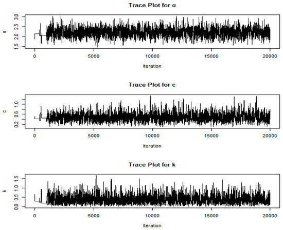
Figure 1. Trace plots of $\alpha , c$ and $k.$

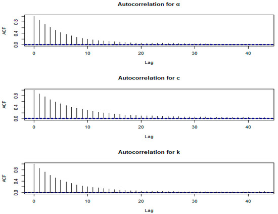
Figure 2. Autocorrelation plots of $\alpha , c$ and $k.$

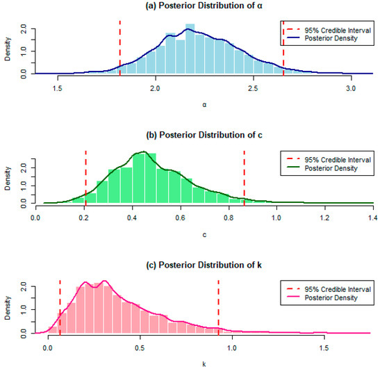
Figure 3. Histogram, posterior density and the lower and upper limits of the 95% credible intervals of $\alpha , c$ and $k.$

Table 10, Table 11, Table 12 and Table 13 present the BPs and BPBs of future observations from the Xg-BXII distribution along with their lengths based on the two-sample prediction scheme and the four priors given in Table 1.

Table 10. Two-sample Bayes predictor and 95% Bayesian prediction bounds of future observations from the Xg-BXII distribution with their lengths under SE and LINEX loss functions for sample sizes $n=30,$ $m=15$ based on prior I.

$\mathbf{s}$	SE Loss Function				LINEX Loss Function
					$\mathit{\nu }\mathbf{=}\mathbf{0.5}$				$\mathit{\nu }\mathbf{=}1.5$
	${\tilde{\mathit{y}}}_{\mathbf{\left(}\mathit{s}\mathbf{\right)}\mathit{S}\mathit{E}}$	$\mathbf{L}\mathbf{L}$	$\mathbf{U}\mathbf{L}$	Length	${\tilde{\mathit{y}}}_{\mathbf{\left(}\mathit{s}\mathbf{\right)}\mathit{L}\mathit{I}\mathit{N}}$	$\mathbf{L}\mathbf{L}$	$\mathbf{U}\mathbf{L}$	Length	${\tilde{\mathit{y}}}_{\mathbf{\left(}\mathit{s}\mathbf{\right)}\mathit{L}\mathit{I}\mathit{N}}$	$\mathbf{L}\mathbf{L}$	$\mathbf{U}\mathbf{L}$	Length
$1$	0.4945	0.4881	0.4999	0.0118	0.4985	0.4944	0.5013	0.0067	0.5011	0.4973	0.5059	0.0086
$8$	0.9042	0.8993	0.9096	0.0103	0.8973	0.8947	0.9003	0.0056	0.9060	0.9022	0.9090	0.0068
$15$	1.5026	1.4991	1.5056	0.0064	1.5013	1.4991	1.5039	0.0048	1.4982	1.4953	1.5008	0.0055

Table 11. Two-sample Bayes predictor and 95% Bayesian prediction bounds of future observations from the Xg-BXII distribution with their lengths under SE and LINEX loss functions for sample sizes $n=30,$ $m=15$ based on Prior II.

$\mathbf{s}$	SE Loss Function				LINEX Loss Function
					$\mathit{\nu }=0.5$				$\mathit{\nu }=1.5$
	${\tilde{\mathit{y}}}_{\left(\mathit{s}\right)\mathit{S}\mathit{E}}$	$\mathbf{L}\mathbf{L}$	$\mathbf{U}\mathbf{L}$	Length	${\tilde{\mathit{y}}}_{\left(\mathit{s}\right)\mathit{L}\mathit{I}\mathit{N}}$	$\mathbf{L}\mathbf{L}$	$\mathbf{U}\mathbf{L}$	Length	${\tilde{\mathit{y}}}_{\left(\mathit{s}\right)\mathit{L}\mathit{I}\mathit{N}}$	$\mathbf{L}\mathbf{L}$	$\mathbf{U}\mathbf{L}$	Length
$1$	0.4985	0.4936	0.5010	0.0074	0.5003	0.4972	0.5034	0.0062	0.4982	0.4952	0.5016	0.0065
$8$	0.9032	0.8995	0.9059	0.0064	0.9006	0.8986	0.9032	0.0047	0.9018	0.8978	0.9041	0.0062
$15$	1.5041	1.5013	1.5075	0.0062	1.4979	1.4956	1.5001	0.0045	1.4980	1.4953	1.5008	0.0055

Table 12. Two-sample Bayes predictor and 95% Bayesian prediction bounds of future observations from the Xg-BXII distribution with their lengths under SE and LINEX loss functions for sample sizes $n=30,$ $m=15$ based on Prior III.

$\mathbf{s}$	SE Loss Function				LINEX Loss Function
					$\mathit{\nu }=0.5$				$\mathit{\nu }=1.5$
	${\tilde{\mathit{y}}}_{\left(\mathit{s}\right)\mathit{S}\mathit{E}}$	$\mathbf{L}\mathbf{L}$	$\mathbf{U}\mathbf{L}$	Length	${\tilde{\mathit{y}}}_{\left(\mathit{s}\right)\mathit{L}\mathit{I}\mathit{N}}$	$\mathbf{L}\mathbf{L}$	$\mathbf{U}\mathbf{L}$	Length	${\tilde{\mathit{y}}}_{\left(\mathit{s}\right)\mathit{L}\mathit{I}\mathit{N}}$	$\mathbf{L}\mathbf{L}$	$\mathbf{U}\mathbf{L}$	Length
$1$	0.5007	0.4972	0.5062	0.0090	0.4992	0.4955	0.5020	0.0065	0.5009	0.4977	0.5055	0.0078
$8$	0.9041	0.8999	0.9075	0.0076	0.8978	0.8941	0.9002	0.0061	0.8995	0.8953	0.9026	0.0072
$15$	1.5010	1.4974	1.5042	0.0068	1.5032	1.4998	1.5055	0.0056	1.5027	1.4998	1.5061	0.0064

Table 13. Two-sample Bayes predictor and 95% Bayesian prediction bounds of future observations from the Xg-BXII distribution with their lengths under SE and LINEX loss functions for sample sizes n = 30, m = 15 based on Prior IV.

$\mathbf{s}$	SE Loss Function				LINEX Loss Function
					$\mathit{\nu }=0.5$				$\mathit{\nu }=1.5$
	${\tilde{\mathit{y}}}_{\left(\mathit{s}\right)\mathit{S}\mathit{E}}$	$\mathbf{L}\mathbf{L}$	$\mathbf{U}\mathbf{L}$	Length	${\tilde{\mathit{y}}}_{\left(\mathit{s}\right)\mathit{L}\mathit{I}\mathit{N}}$	$\mathbf{L}\mathbf{L}$	$\mathbf{U}\mathbf{L}$	Length	${\tilde{\mathit{y}}}_{\left(\mathit{s}\right)\mathit{L}\mathit{I}\mathit{N}}$	$\mathbf{L}\mathbf{L}$	$\mathbf{U}\mathbf{L}$	Length
$1$	0.4996	0.4959	0.5043	0.0085	0.5028	0.4997	0.5048	0.0051	0.5002	0.4985	0.5024	0.0059
$8$	0.8999	0.9011	0.9141	0.0065	0.8994	0.8969	0.9018	0.0049	0.8997	0.8971	0.9022	0.0051
$15$	1.4961	1.4929	1.4989	0.0060	1.4992	1.4971	1.5011	0.0040	1.5004	1.4982	1.5031	0.0049

Concluding remarks

From Table 2, Table 3, Table 4, Table 5, Table 6, Table 7, Table 8 and Table 9, one can note that:

• As the sample size n increases, the PRs of the Bayes estimates of the Xg-BXII distribution parameters decrease, supporting the objective of obtaining reliable parameter estimates for the Xg-BXII distribution, where higher sample sizes allow for better parameter stability.
• For all results, the Bayes estimates under LINEX loss function perform better than the Bayes estimates under the SE loss function. Also, the results under the LINEX loss function with $\nu =0.5$ is better than their corresponding values when using $\nu =1.5$ in terms of having minimum PRs and 95% CI lengths. Moreover, the Bayes estimates under the LINEX loss function with $\nu =0.5$ are quite close to their corresponding estimates under the SE loss function; that is, as $\nu \to 0$, Bayes estimates under LINEX loss function are close to the Bayes estimates under the SE loss function. This suggests that the LINEX loss function may be more suitable for applications where asymmetry in risk is critical, such as engineering risk assessments and survival analysis in medical studies.
• For all results, the Bayes estimates based on Prior II and IV (priors have small variances) perform much better than the Bayes estimates based on Prior I and III (with large variances). This aligns with our objective to provide robust Bayes estimates by selecting informative priors that lead to improved estimation precision, a key consideration in medical and engineering applications, where prior knowledge can significantly influence model performance.
• As the sample size increases, the length of the CIs of the parameters of the Xg-BXII distribution decreases and the CIs turn out to be narrower, reflecting greater confidence in the estimated parameter values. Narrower intervals suggest that the estimates are more precise, meaning there is less variability or that they are spread around the estimated values as the data quantity increases. This behavior is desirable, as it shows the model’s estimates become more stable and dependable with larger data sets.

From Table 10 and Table 13, one can observe the following:

• As $\mathrm{s}$ increases, the BPs under the SE and LINEX loss functions increase.
• For all prediction intervals, the lower and upper bounds and their lengths increase as $\mathrm{s}$ increases; that is, the lower and upper bounds and their length of the first order statistic are less than the lower and upper bounds and their length of the last order statistic.
• The BPs under the SE and LINEX loss functions are included between the lower and upper bounds of all prediction intervals.
• In all cases, the lengths of the BPBs under the LINEX loss function are less than the lengths of the BPBs under the SE loss function.
• The BPs under LINEX loss with $\nu =0.5$ are quite close to the BPs under the SE loss function. Additionally, the BPs under the LINEX loss function with $\nu =1.5$ have the minimum lengths of the BPBs compared to the other BPs.
• The BPs based on Prior II and IV have the minimum lengths of the BPBs compared to the BPs based on Prior I and III.

The results can be summarized as follows:

• The results in Table 10, Table 11, Table 12 and Table 13 show how the BPs change with the ${\mathrm{s}}^{th}$ order statistic. As $\mathrm{s}$ increases, the bounds and lengths of the prediction intervals grow, which is particularly relevant for predicting extreme values, such as the time to last failure in engineering or the longest survival time in a medical context. Notably, the BPs under LINEX loss (with $\nu =0.5$) closely align with those under the SE loss, while offering narrower prediction bounds overall. This result supports the utility of the LINEX loss function for applications that prioritize reduced prediction uncertainty.
• Across all cases, the LINEX loss function outperforms the SE loss function in terms of narrower BPs and CIs, indicating that the LINEX loss function provides more precise prediction. This is especially beneficial in risk-averse applications in engineering and healthcare, where asymmetrical loss can be critical for decision-making.
• The decrease in CIs lengths and narrower CIs as the sample size increases further supports the model’s applicability for large-sample contexts, such as medical and engineering data sets. This finding contributes to our objective of developing a model that can adapt to various sample sizes and produce reliable predictions across different data contexts.

5. Some Applications

This section is devoted to assess the performance of Bayes estimates and predictions through three real-life data sets from engineering and medical applications that have been used by [21] to illustrate the theoretical results in Bayesian inference.

Bayesian estimation and prediction for the Xg-BXII distribution can indeed be applied to both engineering and medical contexts without significant changes to the core functions or estimation approach. However, there may be context-specific differences in the interpretation of parameters and model assumptions: (1) Engineering data often involves precise failure time measurements with potentially lower variability, whereas medical data may have more censoring or variability due to biological factors and patient heterogeneity. (2) The functional form of the hazard rate may vary between contexts based on domain-specific risk factors. For instance, in engineering, hazards often increase over time (e.g., wear-out failures), whereas in medical applications, hazards may be more complex due to age or disease progression. The model can accommodate these differences by selecting context-appropriate baseline hazard functions. (3) When using a Bayesian framework, prior distributions could be adjusted to reflect domain-specific knowledge. For instance, prior information in engineering might be based on historical failure data for specific components, while in medical applications, priors might incorporate clinical or epidemiological data.

5.1. Application 1

This application is given by [2] and represents the time-to-failure data of 18 electronic devices. The data are tabulated in Table 14.

Table 14. Failure times of Wang’s data.

Failure Times
5	11	21	31	46	75	98	122	145
165	196	224	245	293	321	330	350	420

The applicability of the Xg-BXII distribution to this data set has been assessed using the Kolmogorov–Smirnov ($K-S$) test statistic and its corresponding p-value, which were $K-S=0.0980$ and p-value = 0.9883. Based on these results, one can say that the Xg-BXII distribution can be used for modeling this data set.

Bayes estimates and their PRs of the parameters rf, hrf and rhrf of the Xg-BXII distribution for the failure times of Wang’s data are tabulated in Table 15 under SE and LINEX loss functions, where the LINEX loss is used at $\nu =0.5 \mathrm{a}\mathrm{n}\mathrm{d} 1.5$ and time points $\left(x_0=0.5, 1, 2\right)$ are considered. For Bayesian calculation, these combinations of means and variances $\left(1.5, 1.85, 0.3\right)$ and $\left(0.0001, 0.05, 0.001\right)$ was used in calculating the hyperparameters of the joint prior.

Table 15. Bayes estimates and their relevant PRs and 95% credible intervals of the parameters rf, hrf, rhrf of the Xg-BXII distribution along with their lengths under SE and LINEX loss functions for $\left(\nu =0.5,1.5\right)$ and time points $\left(x_0=0.5, 1, 2\right)$ for Wang’s data.

$\underset{\_}{\mathit{\psi }}$	SE		LINEX 0.5		LINEX 1.5		Credible Interval
	Est.	PR	Est.	PR	Est.	PR	Upper	Lower	Width
$\mathit{\alpha }$	1.2460	6.4585 × 10−5	1.2460	1.6146 × 10−5	1.2459	4.8434 × 10−5	1.2615	1.2302	0.0313
$\mathit{c}$	1.2590	0.0260	1.2525	0.0066	1.2398	0.0203	1.5916	0.9603	0.6313
$\mathit{k}$	0.2209	0.0006	0.2208	0.0001	0.2205	0.0004	0.2696	0.1781	0.0914
${\mathit{x}}_{\mathbf{0}}=\mathbf{0.5}$
$\mathit{R}\left({\mathit{x}}_{\mathbf{0}};\underset{\_}{\mathit{\psi }}\right)$	0.6768	7.7331 × 10−5	0.6768	9.6711 × 10−5	0.6768	8.7123 × 10−5	0.6927	0.6581	0.0346
$\mathit{h}\left({\mathit{x}}_{\mathbf{0}};\underset{\_}{\mathit{\psi }}\right)$	0.7481	0.0003	0.7480	3.8414 × 10−5	0.7478	0.0003	0.7844	0.7155	0.0689
$\mathit{r}\left({\mathit{x}}_{\mathbf{0}};\underset{\_}{\mathit{\psi }}\right)$	1.5678	0.0029	1.5671	0.0004	1.5656	0.0033	1.6639	1.4554	0.2086
${\mathit{x}}_{\mathbf{0}}=\mathbf{1}$
$\mathit{R}\left({\mathit{x}}_{\mathbf{0}};\underset{\_}{\mathit{\psi }}\right)$	0.4691	6.5483 × 10−5	0.4691	8.1874 × 10−5	0.5656	7.3723 × 10−5	0.4843	0.4526	0.0317
$\mathit{h}\left({\mathit{x}}_{\mathbf{0}};\underset{\_}{\mathit{\psi }}\right)$	0.7288	0.0004	0.7287	4.9637 × 10−5	0.7285	0.0004	0.7694	0.6924	0.0770
$\mathit{r}\left({\mathit{x}}_{\mathbf{0}};\underset{\_}{\mathit{\psi }}\right)$	0.6440	0.0004	0.6439	4.5553 × 10−5	0.6437	0.0004	0.6813	0.6052	0.0761
${\mathit{x}}_{\mathbf{0}}=\mathbf{2}$
$\mathit{R}\left({\mathit{x}}_{\mathbf{0}};\underset{\_}{\mathit{\psi }}\right)$	0.2208	4.5651 × 10−5	0.6768	9.6711 × 10−5	0.2207	5.1363 × 10−5	0.2337	0.2070	0.0267
$\mathit{h}\left({\mathit{x}}_{\mathbf{0}};\underset{\_}{\mathit{\psi }}\right)$	0.7891	0.0003	0.7890	3.6792 × 10−5	0.7889	0.0003	0.8238	0.7579	0.0659
$\mathit{r}\left({\mathit{x}}_{\mathbf{0}};\underset{\_}{\mathit{\psi }}\right)$	0.2235	2.8757 × 10−5	0.2235	3.5951 × 10−5	0.2235	3.2363 × 10−5	0.2336	0.2127	0.0209

Additionally, Figure 4, Figure 5 and Figure 6 exhibit trace, autocorrelation plots and the histogram of the simulated parameters and the posterior density of each parameter for Wang’s data. These figures include a more detailed description of the trace plots to show convergence, the autocorrelation plots to examine parameter independence, and the histograms and posterior density plots to provide insights into the distribution and behavior of the simulated parameters for Wang’s data.

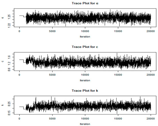
Figure 4. Trace plots of α, c and k for Wang’s data.

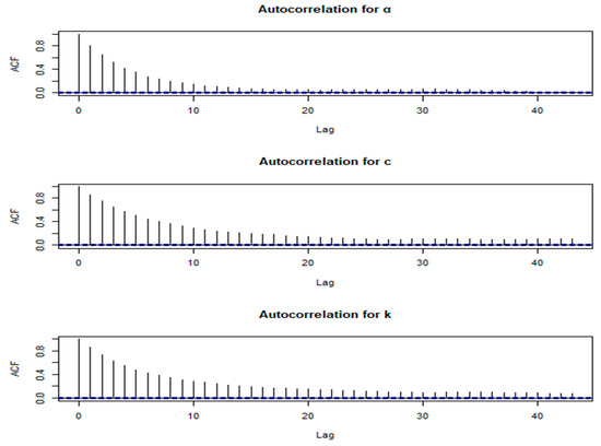
Figure 5. Autocorrelation plots of α, c and k for Wang’s data.

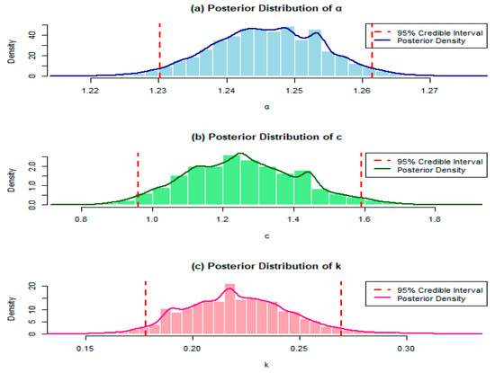
Figure 6. Histogram, posterior density and the lower and upper limits of the 95% credible intervals of the parameters of the Xg-BXII distribution for Wang’s data.

The trace plots display the sampled values of each parameter across iterations in the MCMC simulation. They help assess convergence by showing if the parameter values stabilize over iterations. A well-mixed, stationary trace plot (one without upward or downward trends) suggests that the simulation has likely reached its stationary distribution, indicating reliable parameter estimates.

The autocorrelation plots show the correlation of each parameter with its values from previous iterations (lags). These plots assess the independence of samples. Low autocorrelation at various lags indicates that the samples are relatively independent, improving the efficiency of the MCMC simulation and the quality of the posterior estimates. A high autocorrelation might suggest the need for a longer chain or adjustments to the MCMC algorithm.

The histograms illustrate the distribution of each simulated parameter across all iterations. They provide an empirical view of the parameter distribution, showing the spread and central tendency of the posterior samples. This visual helps assess the variability and potential skewness of each parameter, indicating the range within which the true parameter values likely fall.

The posterior density plots show the estimated posterior density of each parameter. They offer a smoothed view of the parameter’s posterior distribution, giving more precise insight into the probable values of each parameter based on the data. Peaks in the density indicate high-probability values, while the spread reflects parameter uncertainty.

Together, these plots provide a comprehensive view of the parameter behavior, model convergence, and the quality of the posterior estimates for Wang’s data, giving confidence in the robustness and interpretability of the Bayesian model’s results.

Table 16 and Table 17 display the sample size of the first (observed) sample, $n$, and $m$ represents the sample size of the second (future) sample for which the prediction is considered. It denotes the number of new observations that we want to predict based on the information from the first sample. Also, Table 16 and Table 17 show the two-sample Bayesian prediction of $Y_{\left(s\right)}$, where $1\le s\le m$, and a future observation, $Y_{\left(s\right)}$, from a future sample with size $m$ of the time to failure of electronic devices under the SE and LINEX loss functions based on $\left(\nu =0.5, 1.5\right)$. Also, the BPBs and their lengths are presented.

Table 16. Two-sample Bayesian prediction and 95% Bayesian prediction bounds of future observations from the Xg-BXII distribution with their lengths under SE loss function for the failure times of Wang’s data.

$\mathit{n},\mathit{m}$	$\mathbf{s}$	${\tilde{\mathit{y}}}_{\left(\mathit{s}\right)\mathit{S}\mathit{E}}$	Credible Interval
			$\mathbf{L}\mathbf{L}$	$\mathbf{U}\mathbf{L}$	Length
18, 15	$1$	1.9984	1.9963	1.9999	0.0036
	$8$	2.5004	2.4971	2.5031	0.0060
	$15$	3.0028	2.0006	3.0068	0.0062

Table 17. Two-sample Bayesian prediction and 95% Bayesian prediction bounds of future observations from the Xg-BXII distribution with their lengths under LINEX loss function for the failure times of Wang’s data.

$\mathit{n},\mathit{m}$	$\mathbf{s}$	$\mathit{\nu }=0.5$				$\mathit{\nu }=1.5$
		${\tilde{\mathit{y}}}_{\left(\mathit{s}\right)\mathit{L}\mathit{I}\mathit{N}}$	Credible Interval			${\tilde{\mathit{y}}}_{\left(\mathit{s}\right)\mathit{L}\mathit{I}\mathit{N}}$	Credible Interval
			$\mathbf{L}\mathbf{L}$	$\mathbf{U}\mathbf{L}$	Length		$\mathbf{L}\mathbf{L}$	$\mathbf{U}\mathbf{L}$	Length
18, 15	$1$	2.0004	1.9989	2.0018	0.0029	2.0000	1.9985	2.0013	0.0028
	$8$	2.5023	2.4999	2.5054	0.0055	2.5010	2.4988	2.5028	0.0040
	$15$	2.9993	2.9971	3.0024	0.0053	3.0027	3.0001	3.0051	0.0050

5.2. Application 2

This application is given by [39]. The data represent COVID-19 data belonging to the United Kingdom, capturing 76 days, from 15 April to 30 June 2020. The data consist of drought mortality rates. The data are tabulated in Table 18.

Table 18. Drought mortality rates of United Kingdom’s data.

Drought Mortality Rates
0.0587	0.0863	0.1165	0.1247	0.1277	0.1303	0.1652	0.2079	0.2395	0.2751	0.2845
0.2992	0.3188	0.3317	0.3446	0.3553	0.3622	0.3926	0.3629	0.4110	0.4633	0.4690
0.4954	0.5139	0.5696	0.5837	0.6197	0.6365	0.7096	0.7193	0.7444	0.8590	1.0438
1.0602	1.1305	1.1468	1.1533	1.2260	1.2707	1.3423	1.4149	1.5709	1.6017	1.6083
1.6324	1.6998	1.8164	1.8392	1.8721	1.9844	2.1360	2.3987	2.4153	2.5225	2.7087
2.7946	3.3609	3.3715	3.7840	3.9042	4.1969	4.3451	4.4627	4.6477	5.3664	5.4500
5.7522	6.4241	7.0657	7.4456	8.2307	9.6315	10.1870	11.1429	11.2019	22.4584

Based on the value of the $K-S=0.0609$ and its corresponding p-value = 0.9242, one can say that the Xg-BXII distribution provides a good fitting to this real data set.

The Bayes estimates and their PRs of the parameters rf, hrf and rhrf of the Xg-BXII distribution for COVID-19 data from the United Kingdom are tabulated in Table 19 under SE and LINEX loss functions, where the LINEX loss is used at $\nu =0.5 \mathrm{a}\mathrm{n}\mathrm{d} 1.5$ and time points $\left(x_0=0.5, 1, 2\right)$ are considered. For Bayesian calculation, these combinations of means and variances $\left(0.75, 1.5, 0.25\right)$ and $\left(0.005, 0.01, 0.05\right)$ was used to calculate the hyperparameters of the joint prior.

Table 19. Bayes estimates and their relevant standard errors and 95% credible intervals of the parameters of the Xg-BXII distribution along with their lengths under SE loss function for COVID-19 data from the United Kingdom.

$\underset{\_}{\mathit{\psi }}$	SE		LINEX 0.5		LINEX 1.5		Credible Interval
	Est.	PR	Est.	PR	Est.	PR	Upper	Lower	Width
$\mathit{\alpha }$	0.6636	0.0031	0.6628	0.0008	0.6612	0.0024	0.7764	0.5601	0.2163
$\mathit{c}$	1.4589	0.0093	1.4566	0.0023	1.4520	0.0071	1.6529	1.2752	0.3776
$\mathit{k}$	0.2973	0.0112	0.2945	0.0028	0.2891	0.0086	0.5181	0.1111	0.4070
${\mathit{x}}_{\mathbf{0}}=\mathbf{0.5}$
$\mathit{R}\left({\mathit{x}}_{\mathbf{0}};\underset{\_}{\mathit{\psi }}\right)$	0.8063	0.0006	0.8062	7.4504 × 10−5	0.8059	0.0007	0.8477	0.7547	0.0930
$\mathit{h}\left({\mathit{x}}_{\mathbf{0}};\underset{\_}{\mathit{\psi }}\right)$	0.4636	0.0052	0.4623	0.0006	0.4597	0.0058	0.6151	0.3433	0.2718
$\mathit{r}\left({\mathit{x}}_{\mathbf{0}};\underset{\_}{\mathit{\psi }}\right)$	1.9226	0.0061	1.9211	0.0008	1.9181	0.0068	2.0877	1.7807	0.3070
${\mathit{x}}_{\mathbf{0}}=\mathbf{1}$
$\mathit{R}\left({\mathit{x}}_{\mathbf{0}};\underset{\_}{\mathit{\psi }}\right)$	0.6427	0.0017	0.6423	0.0002	0.6415	0.0019	0.7140	0.5596	0.1544
$\mathit{h}\left({\mathit{x}}_{\mathbf{0}};\underset{\_}{\mathit{\psi }}\right)$	0.4466	0.0045	0.4454	0.0006	0.4432	0.0050	0.5863	0.3352	0.2512
$\mathit{r}\left({\mathit{x}}_{\mathbf{0}};\underset{\_}{\mathit{\psi }}\right)$	0.7990	0.0013	0.7986	0.0002	0.7980	0.0015	0.8625	0.7192	0.1433
${\mathit{x}}_{\mathbf{0}}=\mathbf{2}$
$\mathit{R}\left({\mathit{x}}_{\mathbf{0}};\underset{\_}{\mathit{\psi }}\right)$	0.4196	0.0025	0.8062	7.4504 × 10−5	0.4178	0.0028	0.5091	0.3238	0.1853
$\mathit{h}\left({\mathit{x}}_{\mathbf{0}};\underset{\_}{\mathit{\psi }}\right)$	0.4235	0.0025	0.4229	0.0003	0.4217	0.0028	0.5265	0.3374	0.1891
$\mathit{r}\left({\mathit{x}}_{\mathbf{0}};\underset{\_}{\mathit{\psi }}\right)$	0.3045	0.0009	0.3043	0.0001	0.3039	0.0010	0.3608	0.2479	0.1129

Figure 7, Figure 8 and Figure 9 exhibit trace, autocorrelation plots and the histogram of the simulated parameters and the posterior density of each parameter for COVID-19 data from the United Kingdom. The trace plots demonstrate the convergence of the parameters, the autocorrelation plots to assess parameter independence, and the histograms to illustrate the posterior distribution of each parameter for the COVID-19 data. These figures are essential for verifying the stability and reliability of the parameter estimates, which directly support the accuracy and validity of our model as applied to COVID-19 data.

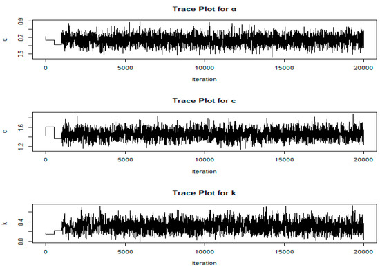
Figure 7. Trace plots of the parameters α, c and k for COVID-19 data from the United Kingdom.

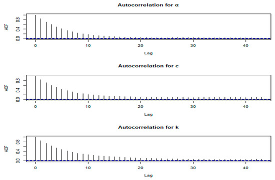
Figure 8. Autocorrelation plots of the parameters α, c and k for COVID-19 data from the United Kingdom.

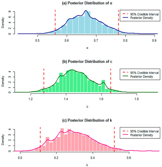
Figure 9. Histogram, posterior density and the lower and upper limits of the 95% credible intervals of the parameters of the Xg-BXII distribution for COVID-19 data from the United Kingdom.

Table 20 and Table 21 display the two-sample Bayesian prediction of $Y_{\left(s\right)}$, where $1\le s\le m$, and a future observation, $Y_{\left(s\right)}$, from a future sample with a size $m$ of drought mortality rates of COVID-19 in the United Kingdom under the SE and LINEX loss functions based on $\left(\nu =0.5, 1.5\right)$. Also, the BPBs and their lengths are presented.

Table 20. Two-sample Bayesian prediction and 95% Bayesian prediction bounds of future observations from the Xg-BXII distribution with their lengths under SE loss function for COVID-19 data from the United Kingdom.

$\mathit{n},\mathit{m}$	$\mathbf{s}$	${\tilde{\mathit{y}}}_{\left(\mathit{s}\right)\mathit{S}\mathit{E}}$	Credible Interval
			$\mathbf{L}\mathbf{L}$	$\mathbf{U}\mathbf{L}$	Length
76, 35	1	0.4996	0.4974	0.5021	0.0047
	18	2.4990	2.4963	2.5016	0.0053
	35	4.0015	3.9993	4.0056	0.0062

Table 21. Two-sample Bayesian prediction and 95% Bayesian prediction bounds of future observations from the Xg-BXII distribution with their lengths under LINEX loss function for COVID-19 data from the United Kingdom.

$\mathit{n},\mathit{m}$	$\mathbf{s}$	$\mathit{\nu }=0.5$				$\mathit{\nu }=1.5$
		${\tilde{\mathit{y}}}_{\left(\mathit{s}\right)\mathit{L}\mathit{I}\mathit{N}}$	Credible Interval			${\tilde{\mathit{y}}}_{\left(\mathit{s}\right)\mathit{L}\mathit{I}\mathit{N}}$	Credible Interval
			$\mathbf{L}\mathbf{L}$	$\mathbf{U}\mathbf{L}$	Length		$\mathbf{L}\mathbf{L}$	$\mathbf{U}\mathbf{L}$	Length
76, 35	$1$	0.4993	0.4966	0.5012	0.0046	0.5022	0.4998	0.5042	0.0044
	$8$	2.4975	2.4949	2.4999	0.0050	2.4999	2.4975	2.5023	0.0048
	$15$	4.0029	3.9998	4.0056	0.0058	4.0008	3.9985	4.0036	0.0052

5.3. Concluding Remarks

From Table 15 and Table 19, it can be concluded that:

• The Bayes estimates of the parameters of the Xg-BXII distribution have smaller PRs and lengths under the LINEX loss function compared to the corresponding results under the SE loss function. This implies that the estimates are closer to the true parameter values on average, making the LINEX loss function a more suitable loss function in situations where asymmetry or skew in errors is important.
• Also, the results under the LINEX loss function when $\nu =0.5$ is greater than when using $\nu =1.5$. This suggests that a lower $\nu$ value makes the LINEX loss function more sensitive to estimation deviations, potentially leading to larger posterior risk and interval lengths. Also, the results of $\nu =0.5$ are close to the results under the SE loss function; this indicates that the LINEX loss function with $\nu =0.5$ behaves more symmetrically, approaching the properties of the SE loss function, which is symmetrical by nature.

Moreover, from Table 16, Table 17, Table 20 and Table 21, it is noticed that:

• As $\mathrm{s}$ increases, the BPs under the SE and LINEX loss functions increase. The increase in the Bayes predictors with higher order statistics $\mathrm{s}$ suggests a positive association between the size of the order statistic $\mathrm{s}$ and the predicted values, reflecting the model’s sensitivity to larger future observations. Moreover, the rate of increase might differ depending on the asymmetry in LINEX, illustrating the effect of different loss function choices on prediction levels.
• For all prediction intervals, the lower and upper bounds and their lengths increase as $\mathrm{s}$ increases. This reflects increased variability or a spread in the distribution at higher order statistics, necessitating wider intervals to represent the range of potential outcomes accurately. The lower and upper bounds and their lengths of the first order statistic are less than the lower and upper bounds and their lengths of the last order statistic; this could be due to the model’s natural behavior or the characteristics of the data set, where extreme values (like the last order statistic) naturally have wider variability.
• The BPs under the SE and LINEX loss functions are included between the lower and upper bounds of all prediction intervals, which suggests that the intervals accurately represent the range of potential outcomes, thereby supporting the reliability of the model’s prediction. Also, it indicates robustness in the model prediction, regardless of the loss function used, including the symmetry (SE) or asymmetry (LINEX) loss functions.
• In all cases, the lengths of the BPBs under the LINEX loss function are shorter than the lengths of the BPBs under the SE loss function. This implies that (1) the shorter lengths of BPBs suggest that the LINEX loss function provides more precise prediction, which can be particularly valuable in decision-making situations where the costs of overestimating or underestimating differ. (2) The narrower predictive bounds under LINEX loss indicate reduced uncertainty in the parameter estimates, which leads to more reliable prediction, making the model more useful for practical applications. (3) It focuses on the importance of selecting a suitable loss function based on the characteristics of the data and the consequences of prediction errors. (4) The choice of the loss function can significantly impact the performance of Bayesian estimation.
• The BPs under LINEX loss with $\nu =0.5$ are quite close to the BPs under the SE loss function; this result highlights that the LINEX loss function behaves similarly to the traditional squared error loss. This indicates that the choice of $\nu$ (which controls the asymmetry of the LINEX loss) can lead to outcomes that are not significantly different from what would be obtained with SE loss function, thereby providing flexibility in loss function selection depending on the problem context.
• Additionally, BPs under the LINEX loss function with $\nu =1.5$ have the minimum lengths of the BPBs compared to the other BPs. This can be explained as a more effective balance between the underestimation and overestimation of parameters, leading to narrower predictive intervals and thus greater confidence in prediction. This result may suggest that when dealing with problems where the cost of underestimating is higher, setting $\nu$ to 1.5 can yield better outcomes. The results underline the importance of carefully selecting not only the loss function but also its parameters. Narrower predictive bounds (especially those under $\nu =1.5$) can lead to improved decision-making in practice, as they reflect greater certainty in the estimated parameters. This can be particularly relevant in fields such as finance, healthcare or engineering, where precise prediction is critical.

6. Conclusions

In this paper, point and interval Bayesian estimation of the parameters of the Xg-BXII distribution are considered under the SE and the LINEX loss functions. Informative independent gamma priors are assumed for the parameters of the Xg-BXII distribution. Moreover, point and interval two-sample Bayesian prediction is presented for future observations from the Xg-BXII distribution. A comprehensive simulation study using the AM algorithm is conducted to evaluate the performance of the Bayes estimates and Bayesian prediction. Based on the simulation results, one can conclude generally that as the sample size increases, the efficiency of the Xg-BXII distribution increases. Also, the Bayes results under the LINEX loss function with a shape parameter near zero are quite close to the Bayes results under the SE loss function. In addition, the Bayes results when assuming priors with small variances are more efficient than priors with large variances. The results are applied to two different applications.

All the results highlight the advantage of using the LINEX loss function in producing more accurate and concise parameter estimates, which may be particularly beneficial for applications sensitive to asymmetrical errors. Also, these findings highlight how tuning the asymmetry parameter $\nu$ affects the balance between sensitivity and precision in the estimates, with lower $\nu$ values yielding results closer to those from the SE loss function. The results demonstrate that higher order statistics in future samples lead to increased Bayes predictions, which can be crucial for applications where large future observations are expected or important to consider. Additionally, these results highlight a positive relationship between $\mathrm{s}$ and the prediction interval width, indicating a broader range of potential values as predictions move from early to later order statistics. These results highlight that the prediction intervals effectively include the Bayes predictors, validating the reliability and robustness of the model’s predictive capability across different loss functions. Moreover, the results illustrate the importance of loss function selection in Bayesian predictive modeling and suggest that the LINEX loss function may lead to better predictive performance in specific applications. The results emphasize the effectiveness of the LINEX loss function with appropriate parameter choices in generating more reliable predictive bounds, contributing to the understanding of Bayesian modeling’s flexibility and applicability in various contexts.

In cases where the sample size is small, the performance of our model may be impacted, potentially leading to wider credible intervals and less precise parameter estimates. Small sample sizes can reduce the informativeness of the data, making the prior assumptions more influential on the posterior results.

Future research could explore the extension of the proposed model to multivariate settings, allowing for the analysis of multiple competing risks simultaneously across various medical and engineering applications. Also, as a future potential work, we may consider the ML, Bayesian estimation and prediction from the Xg-BXII distribution based on record values. Additionally, we may study the ML, Bayesian estimation and prediction for the Xg-BXII distribution based on different types of censoring under different loss functions. Finally, investigating the integration of Bayesian competing risks models with machine learning techniques could lead to more powerful predictive tools, combining the strengths of both approaches.

References

- Xie, M.; Lai, C.D. Reliability analysis using an additive Weibull model with bathtub-shaped failure rate function. Reliab. Eng. Syst. Saf. 1996, 52, 87–93. [Google Scholar] [CrossRef]
- Wang, F.K. A new model with bathtub-shaped failure rate using an additive Burr XII distribution. Reliab. Eng. Syst. Saf. 2000, 70, 305–312. [Google Scholar] [CrossRef]
- Almalki, S.J.; Yuan, J. A new modified Weibull distribution. Reliab. Eng. Syst. Saf. 2013, 111, 164–170. [Google Scholar] [CrossRef]
- He, B.; Cui, W.; Du, X. An additive modified Weibull distribution. Reliab. Eng. Syst. Saf. 2016, 145, 28–37. [Google Scholar] [CrossRef]
- Oluyede, B.O.; Foya, S.; Warahena-Liyanage, G.; Huang, S. The log-logistic Weibull distribution with applications to lifetime data. Austrian J. Stat. 2016, 45, 43–69. [Google Scholar] [CrossRef]
- Singh, B. An additive Perks-Weibull model with bathtub-shaped hazard rate function. Commun. Math. Stat. 2016, 4, 473–493. [Google Scholar] [CrossRef]
- Mdlongwa, P.; Oluyede, B.O.; Amey, A.; Huang, S. The Burr XII modified Weibull distribution: Model, Properties and Applications. Electron. J. Appl. Stat. Anal. 2017, 10, 118–145. [Google Scholar]
- Tarvirdizade, B.; Ahmedpour, M. A new extension of Chen distribution with applications to lifetime data. Math. Stat. 2019, 9, 23–38. [Google Scholar] [CrossRef]
- Shakhatreh, M.K.; Lemonte, A.J.; Moreno-Arenas, G. The log-normal modified Weibull distribution and its reliability implications. Reliab. Eng. Syst. Saf. 2019, 188, 6–22. [Google Scholar] [CrossRef]
- Osagie, S.A.; Osemwenkhae, J.E. Lomax-Weibull distribution with properties and applications in lifetime analysis. Int. J. Math. Anal. Optim. Theory Appl. 2020, 2020, 718–732. [Google Scholar]
- Kamal, R.M.; Ismail, M.A. The flexible Weibull extension-Burr XII distribution: Model, properties and applications. Pak. J. Stat. Oper. Res. 2020, 16, 447–460. [Google Scholar] [CrossRef]
- Thach, T.T.; Bris, R. An additive Chen-Weibull distribution and its applications in reliability modeling. Qual. Reliab. Eng. Int. 2020, 37, 352–373. [Google Scholar] [CrossRef]
- Makubate, B.; Oluyede, B.; Gabanakgosi, M. A new Lindley-Burr XII distribution: Model, Properties and Applications. Int. J. Stat. Probab. 2021, 10, 33–51. [Google Scholar] [CrossRef]
- Abba, B.; Wang, H.; Bakouch, H.S. A reliability and survival model for one and two failure modes system with applications to complete and censored datasets. Reliab. Eng. Syst. Saf. 2022, 223, 108460. [Google Scholar] [CrossRef]
- Xavier, T.; Jose, J.K.; Nadarajah, S. An additive power-transformed half-logistic model and its applications in reliability. Qual. Reliab. Eng. Int. 2022, 38, 3179–3196. [Google Scholar] [CrossRef]
- Thach, T.T. A Three-Component Additive Weibull Distribution and Its Reliability Implications. Symmetry 2022, 14, 1455. [Google Scholar] [CrossRef]
- Salem, H.N.; AL-Dayian, G.R.; EL-Helbawy, A.A.; Abd EL-Kader, R.E. The additive flexible Weibull extension-Lomax distribution: Properties and estimation with applications to COVID-19 data. Acad. Period. Ref. J. AL-Azhar Univ. 2022, 28, 1–44. [Google Scholar] [CrossRef]
- Méndez-González, L.C.; Rodríguez-Picón, L.A.; Pérez Olguínm, I.J.C.; García, V.; Luviano-Cruz, D. The additive Perks distribution and its applications in reliability analysis. Qual. Technol. Quant. Manag. 2022, 20, 784–808. [Google Scholar] [CrossRef]
- Méndez-González, L.C.; Rodríguez-Picón, L.A.; Pérez-Olguín, I.J.C.; Vidal Portilla, L.R. An additive Chen distribution with applications to lifetime data. Axioms 2023, 12, 118. [Google Scholar] [CrossRef]
- Méndez-González, L.C.; Rodríguez-Picón, L.A.; Rodríguez Borbón, M.I.; Sohn, H. The Chen–Perks distribution: Properties and Reliability Applications. Mathematics 2023, 11, 3001. [Google Scholar] [CrossRef]
- Mohammad, H.H.; Alamri, F.S.; Salem, H.N.; EL-Helbawy, A.A. The Additive Xgamma-Burr XII Distribution: Properties, Estimation and Applications. Symmetry 2024, 16, 659. [Google Scholar] [CrossRef]
- Zhao, Y.-G.; Qin, M.-J.; Lu, Z.-H.; Zhang, L.-W. Seismic fragility analysis of nuclear power plants considering structural parameter uncertainty. Reliab. Eng. Syst. Saf. 2021, 216, 107970. [Google Scholar] [CrossRef]
- Zhang, L.-W.; Dang, C.; Zhao, Y.-G. An efficient method for accessing structural reliability indexes via power transformation family. Reliab. Eng. Syst. Saf. 2023, 233, 109097. [Google Scholar] [CrossRef]
- Lawless, J.F. Statistical Models and Methods for Lifetime Data, 2nd ed.; John Wiley & Sons: Hoboken, NJ, USA, 2003. [Google Scholar]
- Gelman, A.; Carlin, J.B.; Stern, H.S.; Dunson, D.B.; Vehtari, A.; Rubin, D.B. Bayesian Data Analysis, 3rd ed.; CRC Press: Boca Raton, FL, USA, 2013. [Google Scholar]
- Varian, H.R. A Bayesian approach to real estate assessment. In Studies in Bayesian Econometrics and Statistics in Honor of Leonard J. Savage; Savage, L.J., Feinberg, S.E., Zellner, A., Eds.; North-Holland Pub. Co.: Amsterdam, The Netherlands, 1975; pp. 195–208. [Google Scholar]
- Zellner, A. Bayesian estimation and prediction using asymmetric loss function. J. Am. Stat. Assoc. 1986, 81, 446–451. [Google Scholar] [CrossRef]
- AL-Hussaini, E.K. Predicting observables from a general class of distributions. J. Stat. Plan. Inference 1999, 79, 79–91. [Google Scholar] [CrossRef]
- Singh, S.K.; Singh, U.; Sharma, V.K. Bayesian estimation and prediction for flexible Weibull model under Type-II censoring scheme. J. Probab. Stat. 2013, 2013, 1–16. [Google Scholar] [CrossRef]
- Wu, M.; Gui, W. Estimation and prediction for Nadarajah-Haghighi distribution under progressive Type-II censoring. Symmetry 2021, 13, 999. [Google Scholar] [CrossRef]
- Ateya, S.F.; Alghamdi, A.S.; Mousa, A.A.A. Future failure time prediction based on a unified hybrid censoring scheme for the Burr-X model with engineering applications. Mathematics 2022, 10, 1450. [Google Scholar] [CrossRef]
- Hasaballah, M.M.; Al-Babtain, A.A.; Hossain, M.M.; Bakr, M.E. Theoretical aspects for Bayesian predictions based on three-parameter Burr-XII distribution and Its applications in climatic data. Symmetry 2023, 15, 1552. [Google Scholar] [CrossRef]
- EL-Helbawy, A.A.; AL-Dayian, G.R.; Salem, H.N.; Abd EL-Kader, R.E. Non-Bayesian and Bayesian prediction for additive flexible Weibull extension-Lomax distribution. J. Econom. Stat. 2024, 4, 79–104. [Google Scholar] [CrossRef]
- Dey, S.; Al-Mosawi, R. Classical and Bayesian Inference of Unit Gompertz Distribution Based on Progressively Type II Censored Data. Am. J. Math. Manag. Sci. 2024, 43, 61–89. [Google Scholar] [CrossRef]
- Berger, J.O. Statistical Decision Theory and Bayesian Analysis; Springer Series in Statistics; Springer: New York, NY, USA, 1985. [Google Scholar]
- Press, S.J. Bayesian Statistics: Principles, Models and Applications; John Wiley and Sons, Inc.: New York, NY, USA, 1989. [Google Scholar]
- Haario, H.; Saksman, E.; Tamminen, J. An adaptive Metropolis algorithm. Bernoulli 2001, 7, 223–242. [Google Scholar] [CrossRef]
- Jaheen, Z.F. Empirical Bayes analysis of record statistics based on LINEX and quadratic loss functions. Comput. Math. Appl. 2004, 47, 947–954. [Google Scholar] [CrossRef]
- Mubarak, A.E.; Almetwally, E.M. A new extension exponential distribution with applications of COVID-19 data. J. Financ. Bus. Res. 2021, 22, 444–460. [Google Scholar]
Disclaimer/Publisher’s Note: The statements, opinions and data contained in all publications are solely those of the individual author(s) and contributor(s) and not of MDPI and/or the editor(s). MDPI and/or the editor(s) disclaim responsibility for any injury to people or property resulting from any ideas, methods, instructions or products referred to in the content. |
© 2024 by the authors. Licensee MDPI, Basel, Switzerland. This article is an open access article distributed under the terms and conditions of the Creative Commons Attribution (CC BY) license (https://creativecommons.org/licenses/by/4.0/).