Author Contributions
Conceptualization, H.H.M. and F.S.A.; methodology, H.H.M., F.S.A., H.N.S. and A.A.E.-H.; software, A.A.E.-H. and H.N.S.; validation, H.N.S. and A.A.E.-H.; formal analysis, H.N.S. and A.A.E.-H.; investigation, H.H.M., F.S.A., H.N.S. and A.A.E.-H.; resources, H.H.M.; data curation, A.A.E.-H. and H.N.S.; writing—original draft preparation, H.H.M. and F.S.A.; writing—review and editing, A.A.E.-H. and H.N.S.; visualization, H.H.M., F.S.A., H.N.S. and A.A.E.-H.; supervision, A.A.E.-H.; project administration, H.H.M. and F.S.A.; funding acquisition, H.H.M. All authors have read and agreed to the published version of the manuscript.
Figure 1.
Trace plots of and
Figure 1.
Trace plots of and
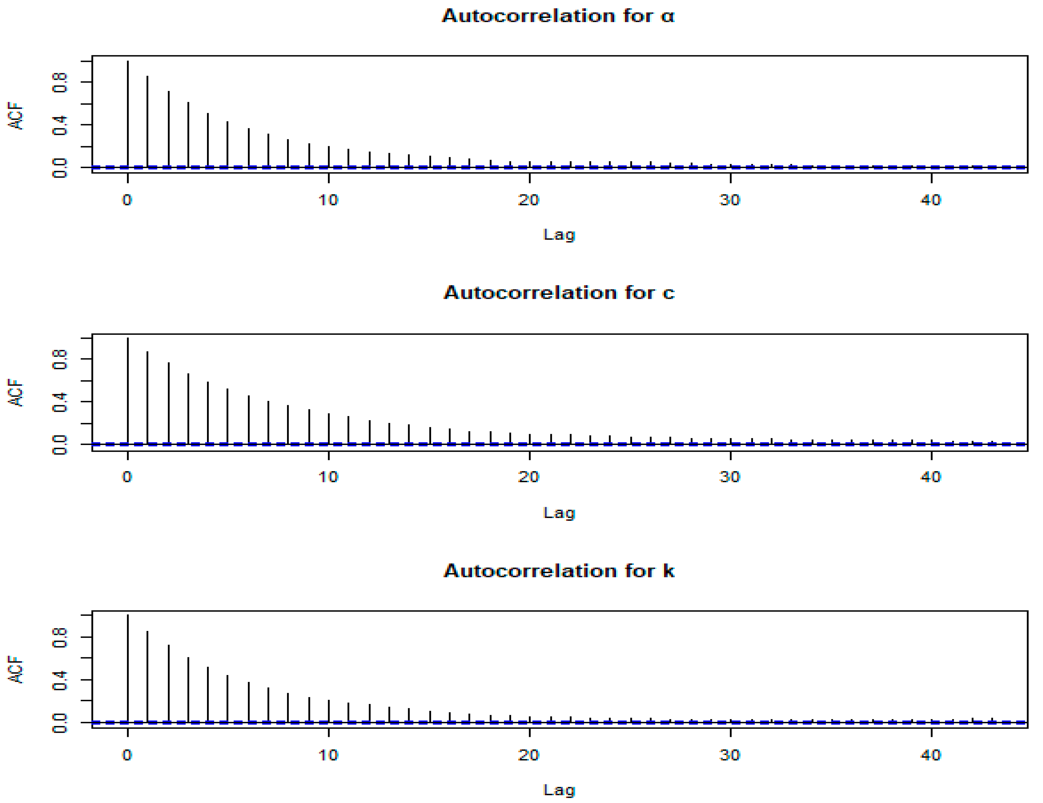
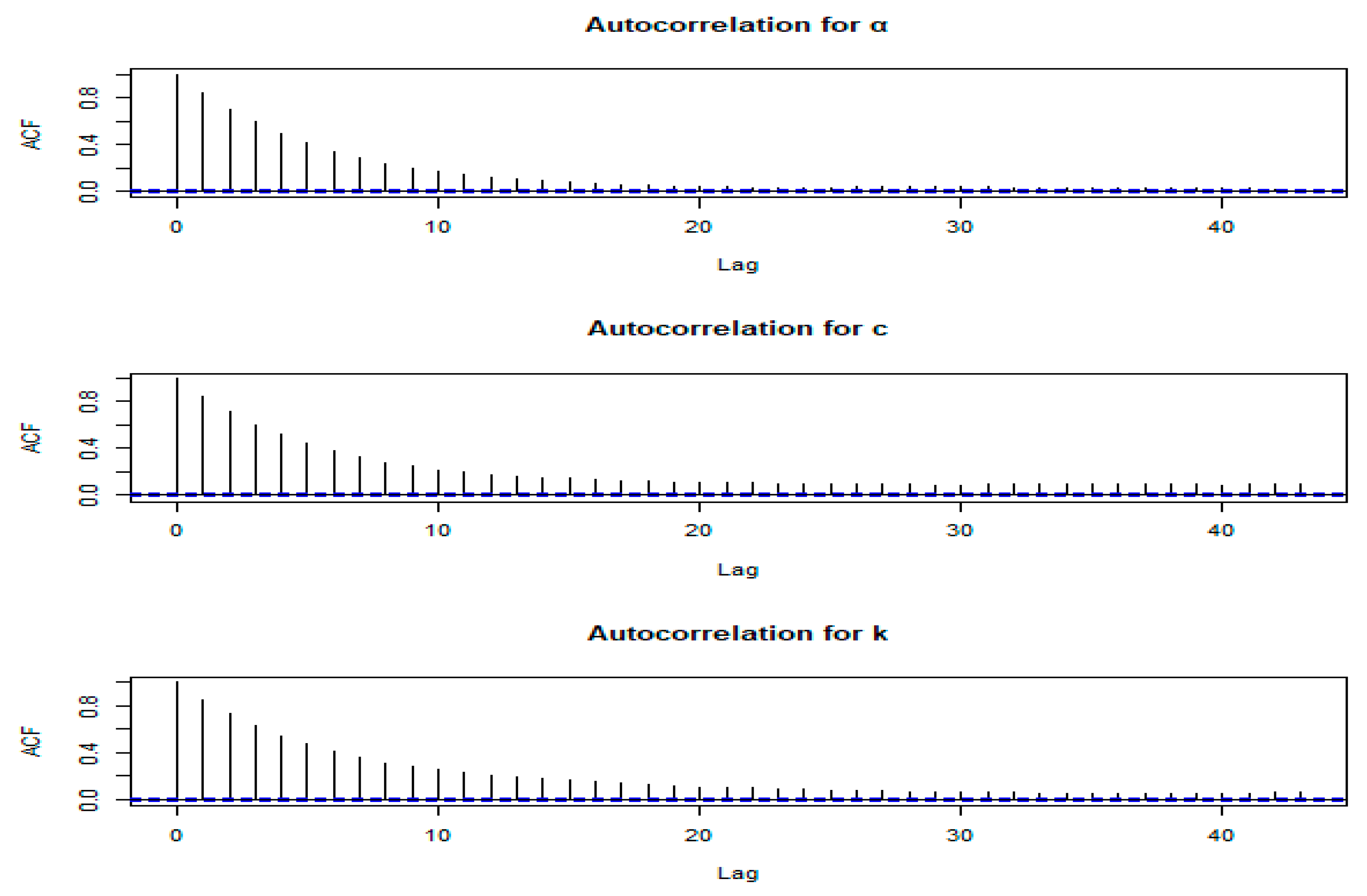
Figure 2.
Autocorrelation plots of and
Figure 2.
Autocorrelation plots of and
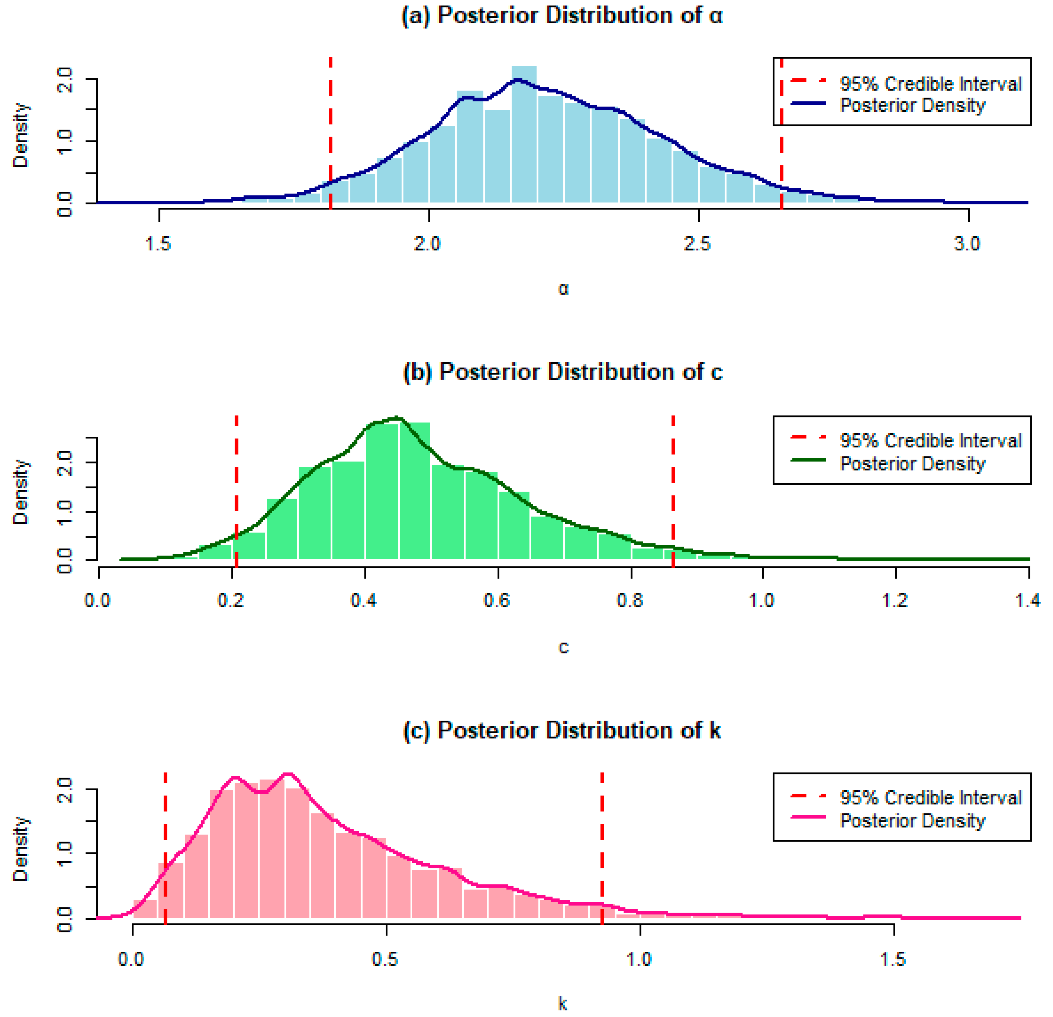
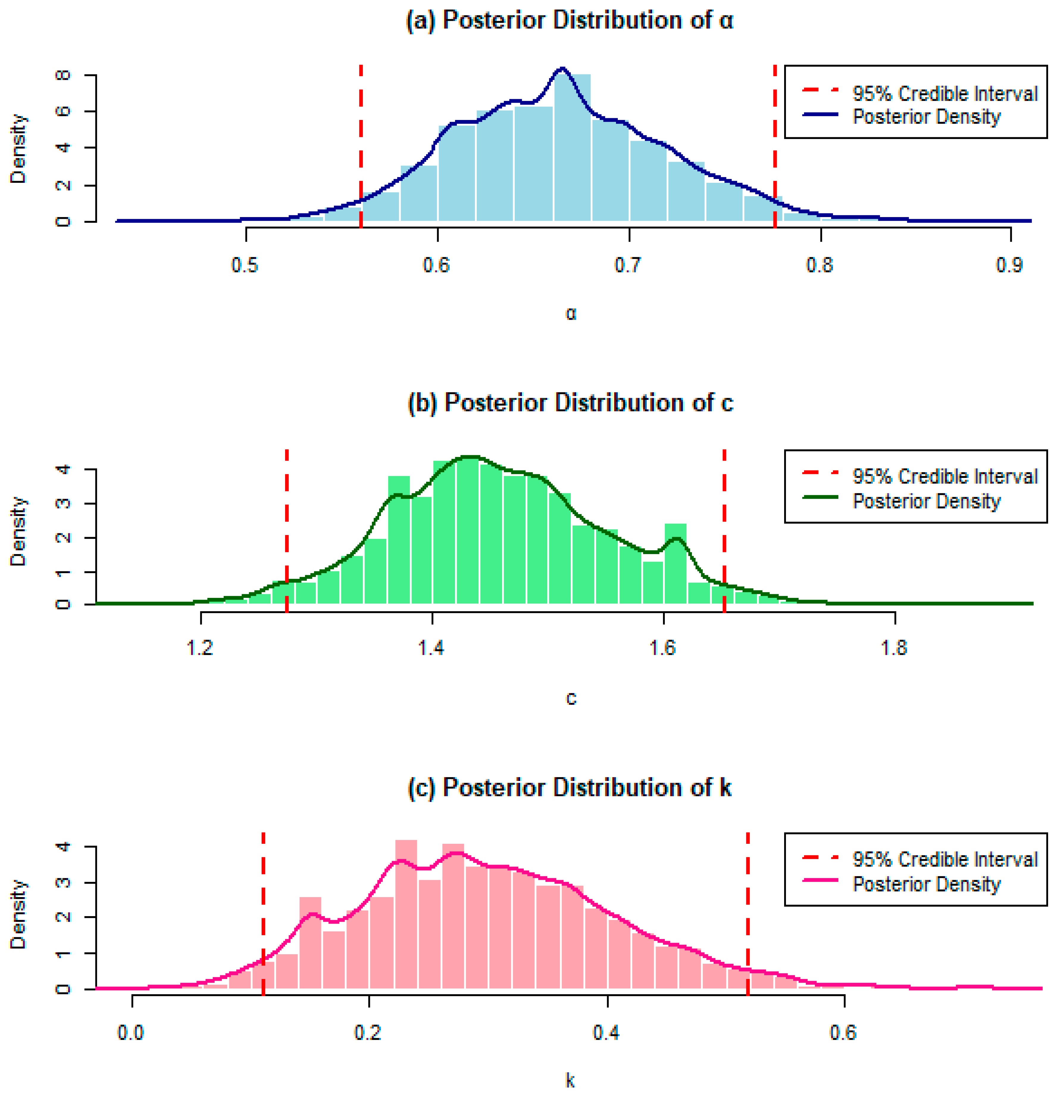
Figure 3.
Histogram, posterior density and the lower and upper limits of the 95% credible intervals of and
Figure 3.
Histogram, posterior density and the lower and upper limits of the 95% credible intervals of and
Figure 4.
Trace plots of α, c and k for Wang’s data.
Figure 4.
Trace plots of α, c and k for Wang’s data.
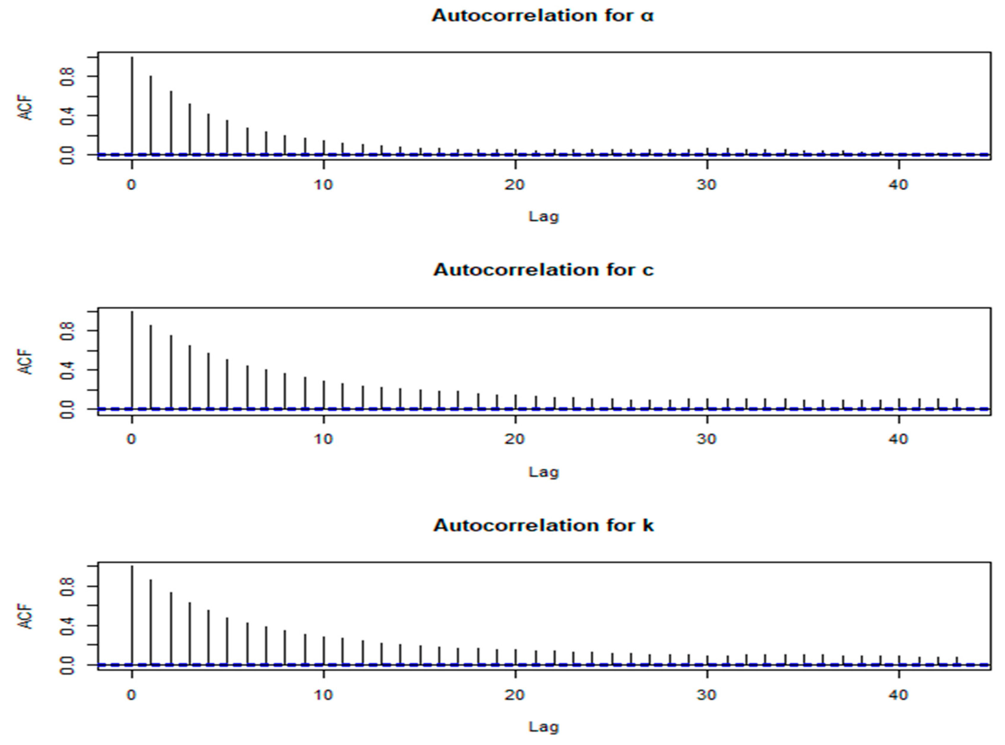
Figure 5.
Autocorrelation plots of α, c and k for Wang’s data.
Figure 5.
Autocorrelation plots of α, c and k for Wang’s data.
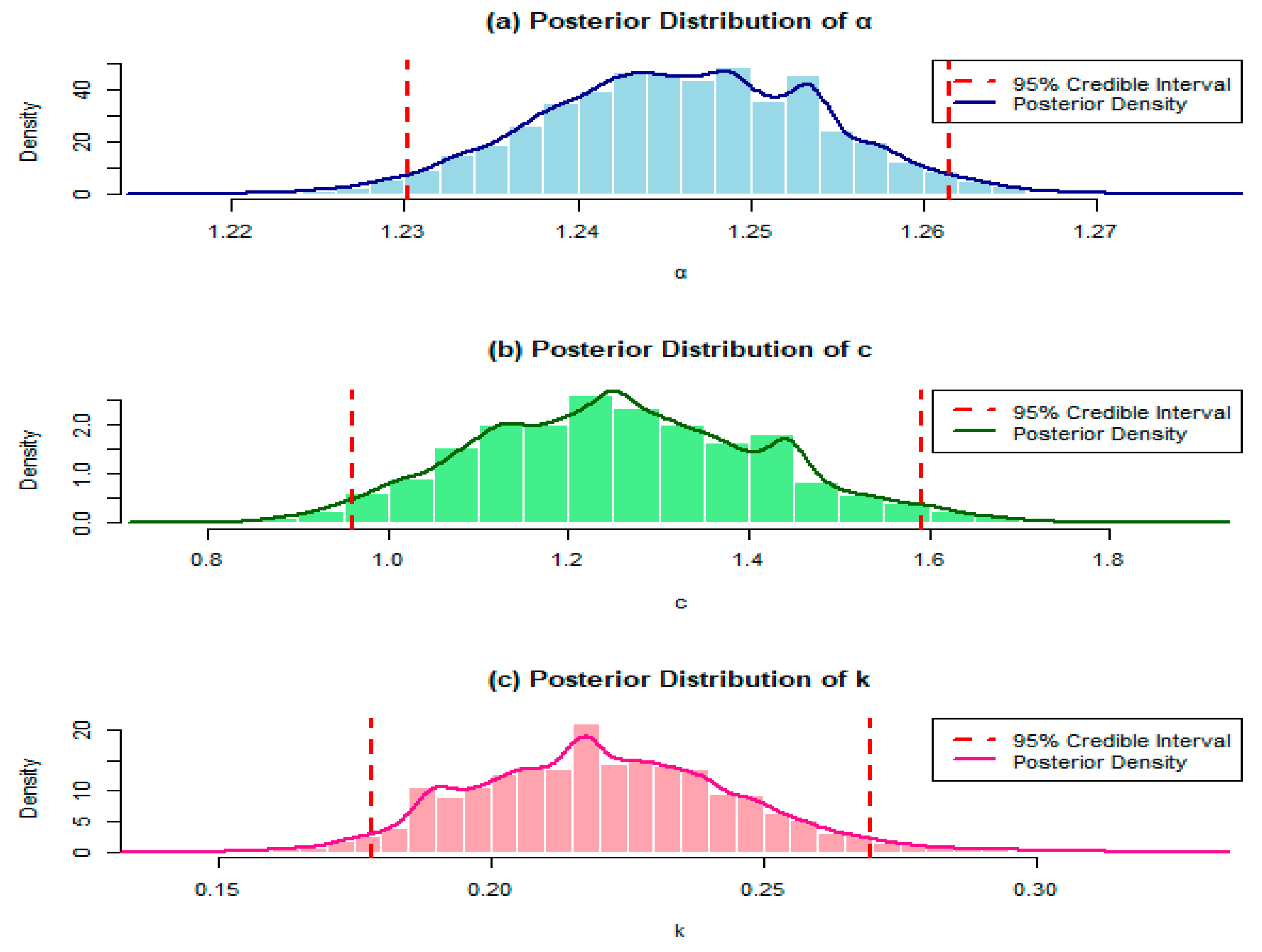
Figure 6.
Histogram, posterior density and the lower and upper limits of the 95% credible intervals of the parameters of the Xg-BXII distribution for Wang’s data.
Figure 6.
Histogram, posterior density and the lower and upper limits of the 95% credible intervals of the parameters of the Xg-BXII distribution for Wang’s data.
Figure 7.
Trace plots of the parameters α, c and k for COVID-19 data from the United Kingdom.
Figure 7.
Trace plots of the parameters α, c and k for COVID-19 data from the United Kingdom.
Figure 8.
Autocorrelation plots of the parameters α, c and k for COVID-19 data from the United Kingdom.
Figure 8.
Autocorrelation plots of the parameters α, c and k for COVID-19 data from the United Kingdom.
Figure 9.
Histogram, posterior density and the lower and upper limits of the 95% credible intervals of the parameters of the Xg-BXII distribution for COVID-19 data from the United Kingdom.
Figure 9.
Histogram, posterior density and the lower and upper limits of the 95% credible intervals of the parameters of the Xg-BXII distribution for COVID-19 data from the United Kingdom.
Table 2.
Bayes estimates and their PRs under the SE and LINEX loss functions for of the parameters of the Xg-BXII distribution and the 95% credible intervals of the parameters along with their lengths based on Priors I and II.
Table 2.
Bayes estimates and their PRs under the SE and LINEX loss functions for of the parameters of the Xg-BXII distribution and the 95% credible intervals of the parameters along with their lengths based on Priors I and II.
| Prior I |
|---|
| n | | SE | LINEX 0.5 | LINEX 1.5 | Credible Interval |
|---|
| Est. | PR | Est. | PR | Est. | PR | UL | LL | Length |
|---|
| 30 | | 2.2174 | 0.0462 | 2.2059 | 0.0118 | 2.1834 | 0.0372 | 2.6544 | 1.8199 | 0.8344 |
| 0.4385 | 0.0276 | 0.4777 | 0.0071 | 0.4649 | 0.0227 | 0.8641 | 0.2071 | 0.6571 |
| 0.3792 | 0.0507 | 0.3671 | 0.0134 | 0.3454 | 0.0454 | 0.9276 | 0.0675 | 0.8601 |
| 60 | | 1.9783 | 0.0288 | 1.9711 | 0.0073 | 1.9570 | 0.0225 | 2.3230 | 1.6630 | 0.6601 |
| 0.5252 | 0.0234 | 0.5194 | 0.0060 | 0.5084 | 0.0189 | 0.8681 | 0.2648 | 0.6033 |
| 0.3083 | 0.0280 | 0.3015 | 0.0072 | 0.2888 | 0.0232 | 0.7002 | 0.0528 | 0.6473 |
| 100 | | 2.0335 | 0.0248 | 2.0273 | 0.0062 | 2.0149 | 0.0191 | 2.3451 | 1.7252 | 0.6200 |
| 0.4685 | 0.0139 | 0.4650 | 0.0035 | 0.4583 | 0.0109 | 0.7160 | 0.2656 | 0.4504 |
| 0.3568 | 0.0255 | 0.3505 | 0.0065 | 0.3385 | 0.0204 | 0.7094 | 0.0784 | 0.6310 |
| Prior II |
| 30 | | 1.9613 | 0.0209 | 1.9561 | 0.0053 | 1.9457 | 0.0161 | 2.2377 | 1.6939 | 0.5438 |
| 0.5082 | 0.0228 | 0.5026 | 0.0059 | 0.4920 | 0.0186 | 0.8544 | 0.2624 | 0.5920 |
| 0.2717 | 0.0203 | 0.2667 | 0.0052 | 0.2575 | 0.0169 | 0.6036 | 0.0686 | 0.5349 |
| 60 | | 1.9956 | 0.0208 | 1.9905 | 0.0052 | 1.9802 | 0.0161 | 2.2898 | 1.7186 | 0.5713 |
| 0.4977 | 0.0148 | 0.4940 | 0.0037 | 0.4869 | 0.0116 | 0.7637 | 0.2881 | 0.4756 |
| 0.3122 | 0.0187 | 0.3076 | 0.0048 | 0.2989 | 0.0151 | 0.6262 | 0.0926 | 0.5336 |
| 100 | | 1.8676 | 0.0150 | 1.8638 | 0.0038 | 1.8563 | 0.0114 | 2.1046 | 1.6011 | 0.5035 |
| 0.4751 | 0.0126 | 0.4719 | 0.0032 | 0.4659 | 0.0098 | 0.7165 | 0.2695 | 0.4470 |
| 0.2530 | 0.0106 | 0.2504 | 0.0027 | 0.2453 | 0.0082 | 0.4755 | 0.0818 | 0.3937 |
Table 3.
Bayes estimates and their PRs under the SE and LINEX loss functions for of the parameters of the Xg-BXII distribution and the 95% credible intervals of the parameters along with their lengths based on Priors III and IV.
Table 3.
Bayes estimates and their PRs under the SE and LINEX loss functions for of the parameters of the Xg-BXII distribution and the 95% credible intervals of the parameters along with their lengths based on Priors III and IV.
| Prior III |
|---|
| n | | SE | LINEX 0.5 | LINEX 1.5 | Credible Interval |
|---|
| Est. | PR | Est. | PR | Est. | PR | UL | LL | Length |
|---|
| 30 | | 0.5159 | 0.0305 | 0.5084 | 0.0078 | 0.4941 | 0.0248 | 0.8989 | 0.2177 | 0.6812 |
| 3.1323 | 0.0455 | 3.1210 | 0.0116 | 3.0989 | 0.0364 | 3.5744 | 2.7345 | 0.8399 |
| 1.6341 | 0.0392 | 1.6244 | 0.0100 | 1.6052 | 0.0311 | 2.0481 | 1.2623 | 0.7858 |
| 60 | | 0.4348 | 0.0223 | 0.4293 | 0.0057 | 0.4186 | 0.0176 | 0.7591 | 0.1767 | 0.5823 |
| 2.9747 | 0.0354 | 2.9659 | 0.0090 | 2.9488 | 0.0282 | 3.3648 | 2.6283 | 0.7366 |
| 1.5338 | 0.0270 | 1.5271 | 0.0068 | 1.5139 | 0.0210 | 1.8613 | 1.2253 | 0.6360 |
| 100 | | 0.4729 | 0.0219 | 0.4674 | 0.0056 | 0.4568 | 0.0172 | 0.7850 | 0.2088 | 0.5762 |
| 2.9057 | 0.0303 | 2.8981 | 0.0077 | 2.8834 | 0.0239 | 3.2679 | 2.5794 | 0.6885 |
| 1.5389 | 0.0210 | 1.5337 | 0.0053 | 1.5233 | 0.0162 | 1.8299 | 1.2576 | 0.5723 |
| Prior IV |
| 30 | | 0.4747 | 0.0218 | 0.4693 | 0.0056 | 0.4590 | 0.0174 | 0.7995 | 0.2308 | 0.5686 |
| 3.0202 | 0.0267 | 3.0136 | 0.0067 | 3.0005 | 0.0208 | 3.3594 | 2.7086 | 0.6508 |
| 1.5676 | 0.0247 | 1.5615 | 0.0062 | 1.5492 | 0.0191 | 1.8813 | 1.2640 | 0.6173 |
| 60 | | 0.4441 | 0.0177 | 0.4397 | 0.0045 | 0.4312 | 0.0140 | 0.7293 | 0.2134 | 0.5159 |
| 3.0618 | 0.0264 | 3.0553 | 0.0067 | 3.0422 | 0.0204 | 3.3914 | 2.7447 | 0.6467 |
| 1.6117 | 0.0209 | 1.6065 | 0.0053 | 1.5962 | 0.0162 | 1.9093 | 1.3369 | 0.5724 |
| 100 | | 0.4179 | 0.0118 | 0.4149 | 0.0030 | 0.4092 | 0.0092 | 0.6526 | 0.2228 | 0.4298 |
| 3.0416 | 0.0218 | 3.0362 | 0.0055 | 3.0255 | 0.0169 | 3.3435 | 2.7619 | 0.5816 |
| 1.5516 | 0.0156 | 1.5477 | 0.0039 | 1.5401 | 0.0121 | 1.8141 | 1.3214 | 0.4927 |
Table 4.
Bayes estimates and their PRs under the SE and LINEX loss functions for of the rf, hrf and rhrf of the Xg-BXII distribution and the 95% credible intervals along with their lengths based on Priors I and II at .
Table 4.
Bayes estimates and their PRs under the SE and LINEX loss functions for of the rf, hrf and rhrf of the Xg-BXII distribution and the 95% credible intervals along with their lengths based on Priors I and II at .
| Prior I |
|---|
| n | rf, hrf
and rhrf | SE | LINEX 0.5 | LINEX 1.5 | Credible Interval |
|---|
| Est. | PR | Est. | PR | Est. | PR | UL | LL | Length |
|---|
| 30 | | 0.4173 | 0.0025 | 0.4167 | 0.0003 | 0.4155 | 0.0028 | 0.5098 | 0.3187 | 0.1911 |
| 1.4318 | 0.0307 | 1.4242 | 0.0038 | 1.4096 | 0.0333 | 1.8060 | 1.1230 | 0.6830 |
| 1.0214 | 0.0143 | 1.0178 | 0.0018 | 1.0106 | 0.0163 | 1.2404 | 0.7675 | 0.4729 |
| 60 | | 0.4753 | 0.0017 | 0.4749 | 0.0002 | 0.4740 | 0.0019 | 0.5525 | 0.3922 | 0.1603 |
| 1.2314 | 0.0158 | 1.2275 | 0.0020 | 1.2197 | 0.0175 | 1.4940 | 1.0057 | 0.4882 |
| 1.1141 | 0.0114 | 1.1112 | 0.0014 | 1.1054 | 0.0130 | 1.3083 | 0.8862 | 0.4220 |
| 100 | | 0.4508 | 0.0012 | 0.4505 | 0.0002 | 0.4498 | 0.0014 | 0.5184 | 0.3852 | 0.1332 |
| 1.2809 | 0.0117 | 1.2780 | 0.0015 | 1.2722 | 0.0130 | 1.5002 | 1.0674 | 0.4328 |
| 1.0506 | 0.0087 | 1.0484 | 0.0011 | 1.0441 | 0.0098 | 1.2280 | 0.8664 | 0.3615 |
| Prior II |
| 30 | | 0.4865 | 0.0017 | 0.4861 | 0.0002 | 0.4852 | 0.0019 | 0.5593 | 0.3994 | 0.1599 |
| 1.1972 | 0.0137 | 1.1938 | 0.0017 | 1.1871 | 0.0152 | 1.4376 | 0.9872 | 0.4504 |
| 1.1339 | 0.0121 | 1.1308 | 0.0015 | 1.1246 | 0.0139 | 1.3159 | 0.8943 | 0.4216 |
| 60 | | 0.4693 | 0.0013 | 0.4690 | 0.0002 | 0.4684 | 0.0014 | 0.5373 | 0.3957 | 0.1417 |
| 1.2388 | 0.0118 | 1.2359 | 0.0015 | 1.2301 | 0.0130 | 1.4628 | 1.0346 | 0.4282 |
| 1.0946 | 0.0084 | 1.0925 | 0.0011 | 1.0883 | 0.0096 | 1.2659 | 0.9048 | 0.3611 |
| 100 | | 0.5075 | 0.0009 | 0.5073 | 0.0001 | 0.5068 | 0.0010 | 0.5656 | 0.4472 | 0.1185 |
| 1.1175 | 0.0075 | 1.1157 | 0.0009 | 1.1119 | 0.0084 | 1.2943 | 0.9389 | 0.3554 |
| 1.1510 | 0.0064 | 1.1494 | 0.0008 | 1.1461 | 0.0073 | 1.3049 | 0.9907 | 0.3142 |
Table 5.
Bayes estimates and their PRs under the SE and LINEX loss functions for of the rf, hrf and rhrf of the Xg-BXII distribution and the 95% credible intervals along with their lengths based on Priors III and IV at .
Table 5.
Bayes estimates and their PRs under the SE and LINEX loss functions for of the rf, hrf and rhrf of the Xg-BXII distribution and the 95% credible intervals along with their lengths based on Priors III and IV at .
| Prior III |
|---|
| n | rf, hrf
and rhrf | SE | LINEX 0.5 | LINEX 1.5 | Credible Interval |
|---|
| Est. | PR | Est. | PR | Est. | PR | UL | LL | Length |
|---|
| 30 | | 0.7692 | 0.0016 | 0.7688 | 0.0002 | 0.7680 | 0.0018 | 0.8414 | 0.6826 | 0.1307 |
| 1.2096 | 0.0241 | 1.2036 | 0.0030 | 1.1918 | 0.0267 | 1.5293 | 0.9183 | 0.5335 |
| 4.0908 | 0.2988 | 4.0169 | 0.0369 | 3.8745 | 0.3243 | 5.1843 | 3.0794 | 2.0174 |
| 60 | | 0.7790 | 0.0010 | 0.7788 | 0.0001 | 0.7782 | 0.0012 | 0.8353 | 0.7103 | 0.1250 |
| 1.1537 | 0.0165 | 1.1496 | 0.0020 | 1.1416 | 0.0183 | 1.4138 | 0.9186 | 0.4953 |
| 4.1063 | 0.2001 | 4.0565 | 0.0249 | 3.9594 | 0.2203 | 4.9936 | 3.2519 | 1.7417 |
| 100 | | 0.7651 | 0.0009 | 0.7649 | 0.0001 | 0.7644 | 0.0010 | 0.8176 | 0.7042 | 0.1134 |
| 1.1937 | 0.0124 | 1.1906 | 0.0015 | 1.1845 | 0.0137 | 1.4312 | 0.9859 | 0.4453 |
| 3.9198 | 0.1615 | 3.8796 | 0.02009 | 3.8012 | 0.1779 | 4.7007 | 3.1627 | 1.5379 |
| Prior IV |
| 30 | | 0.7735 | 0.0011 | 0.7732 | 0.0001 | 0.7726 | 0.0013 | 0.8321 | 0.7020 | 0.1301 |
| 1.1804 | 0.0163 | 1.1763 | 0.0020 | 1.1682 | 0.0182 | 1.4424 | 0.9396 | 0.5028 |
| 4.0707 | 0.1991 | 4.0211 | 0.0248 | 3.9234 | 0.2210 | 4.9373 | 3.2009 | 1.7364 |
| 60 | | 0.7793 | 0.0008 | 0.7791 | 0.0001 | 0.7786 | 0.0009 | 0.8301 | 0.7204 | 0.1097 |
| 1.1822 | 0.0122 | 1.1791 | 0.0015 | 1.1731 | 0.0137 | 1.4096 | 0.9731 | 0.4365 |
| 4.2084 | 0.1767 | 4.1642 | 0.0221 | 4.0759 | 0.1987 | 5.0166 | 3.3794 | 1.6372 |
| 100 | | 0.7881 | 0.0006 | 0.7880 | 7.1641 × 10⁻⁵ | 0.7877 | 0.0006 | 0.8327 | 0.7385 | 0.0942 |
| 1.1361 | 0.0092 | 1.1338 | 0.0011 | 1.1293 | 0.0103 | 1.3313 | 0.9554 | 0.3759 |
| 4.2514 | 0.1304 | 4.2190 | 0.0162 | 4.1554 | 0.1441 | 4.9831 | 3.5544 | 1.4287 |
Table 6.
Bayes estimates and their PRs under the SE and LINEX loss functions for of the rf, hrf and rhrf of the Xg-BXII distribution and the 95% credible intervals along with their lengths based on Priors I and II at .
Table 6.
Bayes estimates and their PRs under the SE and LINEX loss functions for of the rf, hrf and rhrf of the Xg-BXII distribution and the 95% credible intervals along with their lengths based on Priors I and II at .
| Prior I |
|---|
| n | rf, hrf
and rhrf | SE | LINEX 0.5 | LINEX 1.5 | Credible Interval |
|---|
| Est. | PR | Est. | PR | Est. | PR | UL | LL | Length |
|---|
| 30 | | 0.2090 | 0.0016 | 0.2086 | 0.0002 | 0.2078 | 0.0018 | 0.2907 | 0.1355 | 0.1552 |
| 1.4146 | 0.0294 | 1.4073 | 0.0036 | 1.3932 | 0.0321 | 1.7720 | 1.1033 | 0.6687 |
| 0.3687 | 0.0029 | 0.3680 | 0.0004 | 0.3665 | 0.0033 | 0.4696 | 0.2631 | 0.2065 |
| 60 | | 0.2615 | 0.0013 | 0.2612 | 0.0002 | 0.2605 | 0.0015 | 0.1940 | 0.3329 | 0.1389 |
| 1.2119 | 0.0159 | 1.2080 | 0.0020 | 1.2002 | 0.0176 | 0.9820 | 1.4740 | 0.4921 |
| 0.4258 | 0.0021 | 0.4253 | 0.0003 | 0.4242 | 0.0024 | 0.3322 | 0.5144 | 0.1823 |
| 100 | | 0.2419 | 0.0009 | 0.2417 | 0.0001 | 0.2413 | 0.0010 | 0.3018 | 0.1880 | 0.1138 |
| 1.2579 | 0.0123 | 1.2548 | 0.0015 | 1.2487 | 0.0137 | 1.4814 | 1.0458 | 0.4355 |
| 0.3992 | 0.0015 | 0.3988 | 0.0002 | 0.3980 | 0.0017 | 0.4749 | 0.3272 | 0.1477 |
| Prior II |
| 30 | | 0.2717 | 0.0013 | 0.2713 | 0.0002 | 0.2707 | 0.0015 | 0.3411 | 0.2013 | 0.1398 |
| 1.1841 | 0.0131 | 1.1808 | 0.0016 | 1.1743 | 0.0146 | 1.4149 | 0.9761 | 0.4388 |
| 0.4387 | 0.0022 | 0.4381 | 0.0003 | 0.4370 | 0.0025 | 0.5201 | 0.3424 | 0.1777 |
| 60 | | 0.2569 | 0.0010 | 0.2567 | 0.0001 | 0.2562 | 0.0011 | 0.3202 | 0.1978 | 0.1224 |
| 1.2202 | 0.0118 | 1.2173 | 0.0015 | 1.2115 | 0.0131 | 1.4427 | 1.0127 | 0.4300 |
| 0.4193 | 0.0016 | 0.4189 | 0.0002 | 0.4182 | 0.0018 | 0.4952 | 0.3390 | 0.1562 |
| 100 | | 0.2941 | 0.0008 | 0.2939 | 9.9915 × 10⁻⁵ | 0.2935 | 0.0009 | 0.3562 | 0.2397 | 0.1165 |
| 1.1034 | 0.0079 | 1.1015 | 0.0010 | 1.0975 | 0.0089 | 1.2848 | 0.9170 | 0.3678 |
| 0.4577 | 0.0012 | 0.4574 | 0.0001 | 0.4569 | 0.0013 | 0.5252 | 0.3892 | 0.1360 |
Table 7.
Bayes estimates and their PRs under the SE and LINEX loss functions for of the rf, hrf and rhrf of the Xg-BXII distribution and the 95% credible intervals along with their lengths based on Priors III and IV at
Table 7.
Bayes estimates and their PRs under the SE and LINEX loss functions for of the rf, hrf and rhrf of the Xg-BXII distribution and the 95% credible intervals along with their lengths based on Priors III and IV at
| Prior III |
|---|
| n | rf, hrf
and rhrf | SE | LINEX 0.5 | LINEX 1.5 | Credible Interval |
|---|
| Est. | PR | Est. | PR | Est. | PR | UL | LL | Length |
|---|
| 30 | | 0.2759 | 0.0017 | 0.2755 | 0.0002 | 0.2747 | 0.0019 | 0.3648 | 0.1996 | 0.1698 |
| 2.7212 | 0.1300 | 2.6893 | 0.0159 | 2.6291 | 0.1380 | 3.4705 | 2.0726 | 1.1414 |
| 1.0258 | 0.0160 | 1.0219 | 0.0020 | 1.0140 | 0.0177 | 1.2882 | 0.7863 | 0.4930 |
| 60 | | 0.3063 | 0.0013 | 0.3060 | 0.0002 | 0.3054 | 0.0014 | 0.3752 | 0.2389 | 0.1363 |
| 2.4023 | 0.0704 | 2.3849 | 0.0087 | 2.3515 | 0.0762 | 2.9635 | 1.9231 | 1.0404 |
| 1.0540 | 0.0111 | 1.0512 | 0.0014 | 0.0457 | 0.0124 | 1.2601 | 0.8565 | 0.4037 |
| 100 | | 0.2994 | 0.0009 | 0.2992 | 0.0001 | 0.2988 | 0.0010 | 0.3590 | 0.2413 | 0.1176 |
| 2.3733 | 0.0498 | 2.3610 | 0.0062 | 2.3368 | 0.0549 | 2.8262 | 1.9563 | 0.8700 |
| 1.0099 | 0.0081 | 1.0079 | 0.0010 | 1.0039 | 0.0090 | 1.1873 | 0.8405 | 0.3468 |
| Prior IV |
| 30 | | 0.2941 | 0.0013 | 0.2938 | 0.0002 | 0.2931 | 0.0015 | 0.3677 | 0.2272 | 0.1405 |
| 2.5074 | 0.0728 | 2.4893 | 0.0090 | 2.4542 | 0.0797 | 3.0591 | 2.0004 | 1.0587 |
| 1.0375 | 0.0110 | 1.0348 | 0.0014 | 1.0293 | 0.0123 | 1.2486 | 0.8390 | 0.4096 |
| 60 | | 0.2890 | 0.0009 | 0.2888 | 0.0001 | 0.2883 | 0.0010 | 0.3524 | 0.2322 | 0.1202 |
| 2.5930 | 0.0640 | 2.5771 | 0.0079 | 2.5462 | 0.0701 | 3.1102 | 2.1210 | 0.9892 |
| 1.0482 | 0.0084 | 1.0461 | 0.0010 | 1.0419 | 0.0094 | 1.2342 | 0.8748 | 0.3594 |
| 100 | | 0.3049 | 0.0007 | 0.3047 | 9.2821 × 10⁻⁵ | 0.3043 | 0.0008 | 0.3591 | 0.2518 | 0.1073 |
| 2.4722 | 0.0466 | 2.4607 | 0.0058 | 2.4383 | 0.0508 | 2.9304 | 2.0743 | 0.8561 |
| 1.0798 | 0.0067 | 1.0781 | 0.0008 | 1.0748 | 0.0075 | 1.2438 | 0.9231 | 0.3207 |
Table 8.
Bayes estimates and their PRs under the SE and LINEX loss functions for of the rf, hrf and rhrf of the Xg-BXII distribution and the 95% credible intervals along with their lengths based on Priors I and II at .
Table 8.
Bayes estimates and their PRs under the SE and LINEX loss functions for of the rf, hrf and rhrf of the Xg-BXII distribution and the 95% credible intervals along with their lengths based on Priors I and II at .
| Prior I |
|---|
| n | rf, hrf
and rhrf | SE | LINEX 0.5 | LINEX 1.5 | Credible Interval |
|---|
| Est. | PR | Est. | PR | Est. | PR | UL | LL | Length |
|---|
| 30 | | 0.0488 | 0.0003 | 0.4167 | 0.0003 | 0.0486 | 0.0003 | 0.0887 | 0.0215 | 0.0672 |
| 1.5889 | 0.0358 | 1.5800 | 0.0044 | 1.5627 | 0.0392 | 1.9813 | 1.2303 | 0.7509 |
| 0.0788 | 0.0004 | 0.0787 | 5.3681 × 10⁻⁵ | 0.0784 | 0.0005 | 0.1231 | 0.0427 | 0.0804 |
| 60 | | 0.0741 | 0.0004 | 0.4749 | 0.0002 | 0.0738 | 0.0004 | 0.1157 | 0.0419 | 0.0738 |
| 1.3659 | 0.0207 | 1.3607 | 0.0026 | 1.3506 | 0.0229 | 1.6628 | 1.1033 | 0.5594 |
| 0.1070 | 0.0004 | 0.1069 | 4.99 × 10⁻⁵ | 0.1067 | 0.0004 | 0.1469 | 0.0710 | 0.0759 |
| 100 | | 0.0650 | 0.0002 | 0.4505 | 0.0002 | 0.0648 | 0.0002 | 0.0989 | 0.0401 | 0.0588 |
| 1.4158 | 0.0169 | 1.4116 | 0.0021 | 1.4032 | 0.0189 | 1.6767 | 1.1625 | 0.5142 |
| 0.0967 | 0.0002 | 0.0967 | 3.11 × 10⁻⁵ | 0.0966 | 0.0003 | 0.1297 | 0.0684 | 0.0613 |
| Prior II |
| 30 | | 0.0787 | 0.0004 | 0.4861 | 0.0002 | 0.0784 | 0.0004 | 0.1197 | 0.0463 | 0.0734 |
| 1.3416 | 0.0163 | 1.3375 | 0.0020 | 1.3295 | 0.0181 | 1.5923 | 1.1045 | 0.4878 |
| 0.1125 | 0.0004 | 0.1124 | 4.9804 × 10⁻⁵ | 0.1122 | 0.0004 | 0.1523 | 0.0754 | 0.0769 |
| 60 | | 0.0716 | 0.0003 | 0.4690 | 0.0002 | 0.0714 | 0.0003 | 0.1076 | 0.0435 | 0.0641 |
| 1.3775 | 0.0153 | 1.3737 | 0.0019 | 1.3662 | 0.0170 | 1.6328 | 1.1435 | 0.4892 |
| 0.1046 | 0.0003 | 0.1045 | 3.6340 × 10⁻⁵ | 0.1044 | 0.0003 | 0.1398 | 0.0730 | 0.0668 |
| 100 | | 0.0920 | 0.0003 | 0.5073 | 0.0001 | 0.0918 | 0.0003 | 0.1332 | 0.0616 | 0.0716 |
| 1.2532 | 0.0107 | 1.2505 | 0.0013 | 1.2452 | 0.0120 | 1.4563 | 1.0407 | 0.4156 |
| 0.1254 | 0.0003 | 0.1253 | 3.2248 × 10⁻⁵ | 0.1252 | 0.0003 | 0.1617 | 0.0949 | 0.0668 |
Table 9.
Bayes estimates and their PRs under the SE and LINEX loss functions for of the rf, hrf and rhrf of the Xg-BXII distribution and the 95% credible intervals along with their lengths based on Priors III and IV at
Table 9.
Bayes estimates and their PRs under the SE and LINEX loss functions for of the rf, hrf and rhrf of the Xg-BXII distribution and the 95% credible intervals along with their lengths based on Priors III and IV at
| Prior III |
|---|
| n | rf, hrf
and rhrf | SE | LINEX 0.5 | LINEX 1.5 | Credible Interval |
|---|
| Est. | PR | Est. | PR | Est. | PR | UL | LL | Length |
|---|
| 30 | | 0.0195 | 9.9228 × 10⁻⁵ | 0.7688 | 0.0002 | 0.0194 | 0.0001 | 0.0432 | 0.0058 | 0.0604 |
| 2.4823 | 0.1200 | 2.4529 | 0.0147 | 2.3975 | 0.1272 | 3.2180 | 1.8591 | 1.0816 |
| 0.0463 | 0.0003 | 0.0462 | 3.7606 × 10⁻⁵ | 0.0461 | 0.0003 | 0.0857 | 0.0188 | 0.0871 |
| 60 | | 0.0293 | 0.0001 | 0.7788 | 0.0001 | 0.0292 | 0.0001 | 0.0540 | 0.0122 | 0.0418 |
| 2.1612 | 0.0642 | 2.1454 | 0.0079 | 2.1150 | 0.0693 | 2.7062 | 1.7064 | 0.9998 |
| 0.0626 | 0.0003 | 0.0626 | 3.5712 × 10⁻⁵ | 0.0624 | 0.0003 | 0.0978 | 0.0331 | 0.9998 |
| 100 | | 0.0292 | 8.6084 × 10⁻⁵ | 0.7649 | 0.0001 | 0.0292 | 0.0001 | 0.0505 | 0.0142 | 0.0364 |
| 2.1292 | 0.0462 | 2.1177 | 0.0057 | 2.0954 | 0.0507 | 2.5648 | 1.7310 | 0.8338 |
| 0.0623 | 0.0002 | 0.0622 | 2.4922 × 10⁻⁵ | 0.0621 | 0.0002 | 0.0930 | 0.0368 | 0.0562 |
| Prior IV |
| 30 | | 0.0252 | 9.6967 × 10⁻⁵ | 0.7732 | 0.0001 | 0.0251 | 0.0001 | 0.0487 | 0.0105 | 0.0382 |
| 2.2668 | 0.0663 | 2.2504 | 0.0082 | 2.2186 | 0.0724 | 2.7965 | 1.7902 | 1.0063 |
| 0.0562 | 0.0003 | 0.0561 | 3.2118 × 10⁻⁵ | 0.0560 | 0.0003 | 0.0923 | 0.0294 | 0.0628 |
| 60 | | 0.0223 | 6.4644 × 10⁻⁵ | 0.7791 | 0.0001 | 0.0223 | 7.2454 × 10⁻⁵ | 0.0415 | 0.0099 | 0.0315 |
| 2.3458 | 0.0591 | 2.3312 | 0.0073 | 2.3027 | 0.0646 | 2.8462 | 1.8887 | 0.9575 |
| 0.0518 | 0.0002 | 0.0517 | 2.3103 × 10⁻⁵ | 0.0516 | 0.0002 | 0.0826 | 0.0286 | 0.0540 |
| 100 | | 0.0263 | 6.3268 × 10⁻⁵ | 0.7880 | 7.1641 × 10⁻⁵ | 0.0262 | 7.0981 × 10⁻⁵ | 0.0443 | 0.0131 | 0.0312 |
| 2.2311 | 0.0429 | 2.2205 | 0.0053 | 2.1999 | 0.0468 | 2.6659 | 1.8488 | 0.8171 |
| 0.0587 | 0.0002 | 0.0587 | 2.0756 × 10⁻⁵ | 0.0586 | 0.0002 | 0.0862 | 0.0352 | 0.0509 |
Table 10.
Two-sample Bayes predictor and 95% Bayesian prediction bounds of future observations from the Xg-BXII distribution with their lengths under SE and LINEX loss functions for sample sizes based on prior I.
Table 10.
Two-sample Bayes predictor and 95% Bayesian prediction bounds of future observations from the Xg-BXII distribution with their lengths under SE and LINEX loss functions for sample sizes based on prior I.
| SE Loss Function | LINEX Loss Function |
|---|
| |
|---|
| | | Length | | | | Length | | | | Length |
|---|
| 0.4945 | 0.4881 | 0.4999 | 0.0118 | 0.4985 | 0.4944 | 0.5013 | 0.0067 | 0.5011 | 0.4973 | 0.5059 | 0.0086 |
| 0.9042 | 0.8993 | 0.9096 | 0.0103 | 0.8973 | 0.8947 | 0.9003 | 0.0056 | 0.9060 | 0.9022 | 0.9090 | 0.0068 |
| 1.5026 | 1.4991 | 1.5056 | 0.0064 | 1.5013 | 1.4991 | 1.5039 | 0.0048 | 1.4982 | 1.4953 | 1.5008 | 0.0055 |
Table 11.
Two-sample Bayes predictor and 95% Bayesian prediction bounds of future observations from the Xg-BXII distribution with their lengths under SE and LINEX loss functions for sample sizes based on Prior II.
Table 11.
Two-sample Bayes predictor and 95% Bayesian prediction bounds of future observations from the Xg-BXII distribution with their lengths under SE and LINEX loss functions for sample sizes based on Prior II.
| SE Loss Function | LINEX Loss Function |
|---|
| |
|---|
| | | Length | | | | Length | | | | Length |
|---|
| 0.4985 | 0.4936 | 0.5010 | 0.0074 | 0.5003 | 0.4972 | 0.5034 | 0.0062 | 0.4982 | 0.4952 | 0.5016 | 0.0065 |
| 0.9032 | 0.8995 | 0.9059 | 0.0064 | 0.9006 | 0.8986 | 0.9032 | 0.0047 | 0.9018 | 0.8978 | 0.9041 | 0.0062 |
| 1.5041 | 1.5013 | 1.5075 | 0.0062 | 1.4979 | 1.4956 | 1.5001 | 0.0045 | 1.4980 | 1.4953 | 1.5008 | 0.0055 |
Table 12.
Two-sample Bayes predictor and 95% Bayesian prediction bounds of future observations from the Xg-BXII distribution with their lengths under SE and LINEX loss functions for sample sizes based on Prior III.
Table 12.
Two-sample Bayes predictor and 95% Bayesian prediction bounds of future observations from the Xg-BXII distribution with their lengths under SE and LINEX loss functions for sample sizes based on Prior III.
| SE Loss Function | LINEX Loss Function |
|---|
| |
|---|
| | | Length | | | | Length | | | | Length |
|---|
| 0.5007 | 0.4972 | 0.5062 | 0.0090 | 0.4992 | 0.4955 | 0.5020 | 0.0065 | 0.5009 | 0.4977 | 0.5055 | 0.0078 |
| 0.9041 | 0.8999 | 0.9075 | 0.0076 | 0.8978 | 0.8941 | 0.9002 | 0.0061 | 0.8995 | 0.8953 | 0.9026 | 0.0072 |
| 1.5010 | 1.4974 | 1.5042 | 0.0068 | 1.5032 | 1.4998 | 1.5055 | 0.0056 | 1.5027 | 1.4998 | 1.5061 | 0.0064 |
Table 13.
Two-sample Bayes predictor and 95% Bayesian prediction bounds of future observations from the Xg-BXII distribution with their lengths under SE and LINEX loss functions for sample sizes n = 30, m = 15 based on Prior IV.
Table 13.
Two-sample Bayes predictor and 95% Bayesian prediction bounds of future observations from the Xg-BXII distribution with their lengths under SE and LINEX loss functions for sample sizes n = 30, m = 15 based on Prior IV.
| SE Loss Function | LINEX Loss Function |
|---|
| |
|---|
| | |
Length | | | |
Length | | | |
Length |
|---|
| 0.4996 | 0.4959 | 0.5043 | 0.0085 | 0.5028 | 0.4997 | 0.5048 | 0.0051 | 0.5002 | 0.4985 | 0.5024 | 0.0059 |
| 0.8999 | 0.9011 | 0.9141 | 0.0065 | 0.8994 | 0.8969 | 0.9018 | 0.0049 | 0.8997 | 0.8971 | 0.9022 | 0.0051 |
| 1.4961 | 1.4929 | 1.4989 | 0.0060 | 1.4992 | 1.4971 | 1.5011 | 0.0040 | 1.5004 | 1.4982 | 1.5031 | 0.0049 |
Table 14.
Failure times of Wang’s data.
Table 14.
Failure times of Wang’s data.
| Failure Times |
| 5 | 11 | 21 | 31 | 46 | 75 | 98 | 122 | 145 |
| 165 | 196 | 224 | 245 | 293 | 321 | 330 | 350 | 420 |
Table 15.
Bayes estimates and their relevant PRs and 95% credible intervals of the parameters rf, hrf, rhrf of the Xg-BXII distribution along with their lengths under SE and LINEX loss functions for and time points for Wang’s data.
Table 15.
Bayes estimates and their relevant PRs and 95% credible intervals of the parameters rf, hrf, rhrf of the Xg-BXII distribution along with their lengths under SE and LINEX loss functions for and time points for Wang’s data.
| SE | LINEX 0.5 | LINEX 1.5 | Credible Interval |
|---|
| Est. | PR | Est. | PR | Est. | PR | Upper | Lower | Width |
|---|
| 1.2460 | 6.4585 × 10⁻⁵ | 1.2460 | 1.6146 × 10⁻⁵ | 1.2459 | 4.8434 × 10⁻⁵ | 1.2615 | 1.2302 | 0.0313 |
| 1.2590 | 0.0260 | 1.2525 | 0.0066 | 1.2398 | 0.0203 | 1.5916 | 0.9603 | 0.6313 |
| 0.2209 | 0.0006 | 0.2208 | 0.0001 | 0.2205 | 0.0004 | 0.2696 | 0.1781 | 0.0914 |
|
| 0.6768 | 7.7331 × 10⁻⁵ | 0.6768 | 9.6711 × 10⁻⁵ | 0.6768 | 8.7123 × 10⁻⁵ | 0.6927 | 0.6581 | 0.0346 |
| 0.7481 | 0.0003 | 0.7480 | 3.8414 × 10⁻⁵ | 0.7478 | 0.0003 | 0.7844 | 0.7155 | 0.0689 |
| 1.5678 | 0.0029 | 1.5671 | 0.0004 | 1.5656 | 0.0033 | 1.6639 | 1.4554 | 0.2086 |
|
| 0.4691 | 6.5483 × 10⁻⁵ | 0.4691 | 8.1874 × 10⁻⁵ | 0.5656 | 7.3723 × 10⁻⁵ | 0.4843 | 0.4526 | 0.0317 |
| 0.7288 | 0.0004 | 0.7287 | 4.9637 × 10⁻⁵ | 0.7285 | 0.0004 | 0.7694 | 0.6924 | 0.0770 |
| 0.6440 | 0.0004 | 0.6439 | 4.5553 × 10⁻⁵ | 0.6437 | 0.0004 | 0.6813 | 0.6052 | 0.0761 |
|
| 0.2208 | 4.5651 × 10⁻⁵ | 0.6768 | 9.6711 × 10⁻⁵ | 0.2207 | 5.1363 × 10⁻⁵ | 0.2337 | 0.2070 | 0.0267 |
| 0.7891 | 0.0003 | 0.7890 | 3.6792 × 10⁻⁵ | 0.7889 | 0.0003 | 0.8238 | 0.7579 | 0.0659 |
| 0.2235 | 2.8757 × 10⁻⁵ | 0.2235 | 3.5951 × 10⁻⁵ | 0.2235 | 3.2363 × 10⁻⁵ | 0.2336 | 0.2127 | 0.0209 |
Table 16.
Two-sample Bayesian prediction and 95% Bayesian prediction bounds of future observations from the Xg-BXII distribution with their lengths under SE loss function for the failure times of Wang’s data.
Table 16.
Two-sample Bayesian prediction and 95% Bayesian prediction bounds of future observations from the Xg-BXII distribution with their lengths under SE loss function for the failure times of Wang’s data.
| | | Credible Interval |
|---|
| | Length |
|---|
| 18, 15 | | 1.9984 | 1.9963 | 1.9999 | 0.0036 |
| 2.5004 | 2.4971 | 2.5031 | 0.0060 |
| 3.0028 | 2.0006 | 3.0068 | 0.0062 |
Table 17.
Two-sample Bayesian prediction and 95% Bayesian prediction bounds of future observations from the Xg-BXII distribution with their lengths under LINEX loss function for the failure times of Wang’s data.
Table 17.
Two-sample Bayesian prediction and 95% Bayesian prediction bounds of future observations from the Xg-BXII distribution with their lengths under LINEX loss function for the failure times of Wang’s data.
| | | |
|---|
| Credible Interval | | Credible Interval |
|---|
| | Length | | | Length |
|---|
| 18, 15 | | 2.0004 | 1.9989 | 2.0018 | 0.0029 | 2.0000 | 1.9985 | 2.0013 | 0.0028 |
| 2.5023 | 2.4999 | 2.5054 | 0.0055 | 2.5010 | 2.4988 | 2.5028 | 0.0040 |
| 2.9993 | 2.9971 | 3.0024 | 0.0053 | 3.0027 | 3.0001 | 3.0051 | 0.0050 |
Table 18.
Drought mortality rates of United Kingdom’s data.
Table 18.
Drought mortality rates of United Kingdom’s data.
| Drought Mortality Rates |
| 0.0587 | 0.0863 | 0.1165 | 0.1247 | 0.1277 | 0.1303 | 0.1652 | 0.2079 | 0.2395 | 0.2751 | 0.2845 |
| 0.2992 | 0.3188 | 0.3317 | 0.3446 | 0.3553 | 0.3622 | 0.3926 | 0.3629 | 0.4110 | 0.4633 | 0.4690 |
| 0.4954 | 0.5139 | 0.5696 | 0.5837 | 0.6197 | 0.6365 | 0.7096 | 0.7193 | 0.7444 | 0.8590 | 1.0438 |
| 1.0602 | 1.1305 | 1.1468 | 1.1533 | 1.2260 | 1.2707 | 1.3423 | 1.4149 | 1.5709 | 1.6017 | 1.6083 |
| 1.6324 | 1.6998 | 1.8164 | 1.8392 | 1.8721 | 1.9844 | 2.1360 | 2.3987 | 2.4153 | 2.5225 | 2.7087 |
| 2.7946 | 3.3609 | 3.3715 | 3.7840 | 3.9042 | 4.1969 | 4.3451 | 4.4627 | 4.6477 | 5.3664 | 5.4500 |
| 5.7522 | 6.4241 | 7.0657 | 7.4456 | 8.2307 | 9.6315 | 10.1870 | 11.1429 | 11.2019 | 22.4584 | |
Table 19.
Bayes estimates and their relevant standard errors and 95% credible intervals of the parameters of the Xg-BXII distribution along with their lengths under SE loss function for COVID-19 data from the United Kingdom.
Table 19.
Bayes estimates and their relevant standard errors and 95% credible intervals of the parameters of the Xg-BXII distribution along with their lengths under SE loss function for COVID-19 data from the United Kingdom.
| SE | LINEX 0.5 | LINEX 1.5 | Credible Interval |
|---|
| Est. | PR | Est. | PR | Est. | PR | Upper | Lower | Width |
|---|
| 0.6636 | 0.0031 | 0.6628 | 0.0008 | 0.6612 | 0.0024 | 0.7764 | 0.5601 | 0.2163 |
| 1.4589 | 0.0093 | 1.4566 | 0.0023 | 1.4520 | 0.0071 | 1.6529 | 1.2752 | 0.3776 |
| 0.2973 | 0.0112 | 0.2945 | 0.0028 | 0.2891 | 0.0086 | 0.5181 | 0.1111 | 0.4070 |
|
| 0.8063 | 0.0006 | 0.8062 | 7.4504 × 10⁻⁵ | 0.8059 | 0.0007 | 0.8477 | 0.7547 | 0.0930 |
| 0.4636 | 0.0052 | 0.4623 | 0.0006 | 0.4597 | 0.0058 | 0.6151 | 0.3433 | 0.2718 |
| 1.9226 | 0.0061 | 1.9211 | 0.0008 | 1.9181 | 0.0068 | 2.0877 | 1.7807 | 0.3070 |
|
| 0.6427 | 0.0017 | 0.6423 | 0.0002 | 0.6415 | 0.0019 | 0.7140 | 0.5596 | 0.1544 |
| 0.4466 | 0.0045 | 0.4454 | 0.0006 | 0.4432 | 0.0050 | 0.5863 | 0.3352 | 0.2512 |
| 0.7990 | 0.0013 | 0.7986 | 0.0002 | 0.7980 | 0.0015 | 0.8625 | 0.7192 | 0.1433 |
|
| 0.4196 | 0.0025 | 0.8062 | 7.4504 × 10⁻⁵ | 0.4178 | 0.0028 | 0.5091 | 0.3238 | 0.1853 |
| 0.4235 | 0.0025 | 0.4229 | 0.0003 | 0.4217 | 0.0028 | 0.5265 | 0.3374 | 0.1891 |
| 0.3045 | 0.0009 | 0.3043 | 0.0001 | 0.3039 | 0.0010 | 0.3608 | 0.2479 | 0.1129 |
Table 20.
Two-sample Bayesian prediction and 95% Bayesian prediction bounds of future observations from the Xg-BXII distribution with their lengths under SE loss function for COVID-19 data from the United Kingdom.
Table 20.
Two-sample Bayesian prediction and 95% Bayesian prediction bounds of future observations from the Xg-BXII distribution with their lengths under SE loss function for COVID-19 data from the United Kingdom.
| | | Credible Interval |
|---|
| | Length |
|---|
| 76, 35 | 1 | 0.4996 | 0.4974 | 0.5021 | 0.0047 |
| 18 | 2.4990 | 2.4963 | 2.5016 | 0.0053 |
| 35 | 4.0015 | 3.9993 | 4.0056 | 0.0062 |
Table 21.
Two-sample Bayesian prediction and 95% Bayesian prediction bounds of future observations from the Xg-BXII distribution with their lengths under LINEX loss function for COVID-19 data from the United Kingdom.
Table 21.
Two-sample Bayesian prediction and 95% Bayesian prediction bounds of future observations from the Xg-BXII distribution with their lengths under LINEX loss function for COVID-19 data from the United Kingdom.
| | | |
|---|
| Credible Interval | | Credible Interval |
|---|
| | Length | | | Length |
|---|
| 76, 35 | | 0.4993 | 0.4966 | 0.5012 | 0.0046 | 0.5022 | 0.4998 | 0.5042 | 0.0044 |
| 2.4975 | 2.4949 | 2.4999 | 0.0050 | 2.4999 | 2.4975 | 2.5023 | 0.0048 |
| 4.0029 | 3.9998 | 4.0056 | 0.0058 | 4.0008 | 3.9985 | 4.0036 | 0.0052 |


