Effective Quantum Field Theory Methods for Calculating Feynman Integrals

Abstract

A review of modern methods for effective calculations of Feynman integrals containing both massless propagators and propagators with masses is given. The effectiveness of these methods in various fields of their application is demonstrated by the examples under consideration.

1. Introduction

Currently, perturbation theory (PT) provides basic information about both the processes studied in experiments and the properties of the physical models themselves. The matrix elements in the cross-sections of the processes depend on the masses of the interacting particles, and therefore, strictly speaking, require the calculation of Feynman integrals (FIs) containing massive propagators. However, depending on the kinematics of the processes under study, the values of some masses can be set to zero, and then the FI calculation is greatly simplified.

Studying the properties of the physical models themselves, such as critical indices, anomalous dimensions for particles, and operators, requires the calculations of massless FIs, whose results contain fairly simple structures. These results can be obtained in PT high orders.

FI calculations are preferably, if possible, analytical methods, since numerical methods rarely have sufficiently high accuracy. In addition, numerical methods for calculating diagrams are often inapplicable due to the singularities they contain and (which is especially important for gauge theories) due to mutual reductions between the contributions of different integrals and even between different parts of the same integral.

Moreover, accurate results are often needed. For example, when calculating renormalizations in theories with high internal symmetry, it is important to know [1] the positions of critical points in which the found $\beta$ functions have zero values in the appropriate PT order.

I would like to draw attention to the fact that the main objects of calculations are scalar diagrams. Therefore, within the framework of dimensional regularization [2,3,4,5], where diagrams are calculated for an arbitrary dimension of space, the FIs found for any model (or process) can be easily used in the study of other models (and processes). As a result, the complexity of the analytical FI calculations is compensated by the possibility of their application in various quantum field models.

We also note that sometimes the result of FI calculations may be of independent interest. So, for example, when using non-trivial identities such as the “uniqueness” relation [6,7], the results appear (see [8,9,10,11,12,13]) for some integrals and/or series that are not available in the reference literature. For example, the calculation of the same FI performed in [8,9,10,11,12] and [14] using various calculation methods, led to a previously unknown relation between ${}_3{F}_2$-hypergeometric functions with arguments 1 and $-1$. This ratio was neatly proven only very recently [15].

Now there are many powerful methods for calculating the Feynman diagrams of a certain type (in the massless and massive cases (see, in particular, recent reviews in [16,17], respectively), which are often inferior in breadth of use to standard methods such as $\alpha$-representation and the Feynman parameter method (see, for example, [1,18]); however, this lead to significant progress in studying specific processes (or quantities).

In this review, we will present methods based on integration by parts (IBP) [7,19], on functional relations (FRs) [20,21,22], and on differential equations (DEs) [23,24,25,26,27,28,29], which are conveniently applicable when calculating both massless diagrams and diagrams with massive propagators. In the massless case, we will consider, in particular, diagrams giving contributions to the coefficient functions and anomalous dimensions of Wilson operators in the framework of deep inelastic scattering (DIS) of leptons on hadrons (see Section 1, Section 2, Section 3 and Section 4).

Moreover, we will also consider the basic diagrams that contribute to the $\beta$ function of the ${\phi }^4$ model, two of which will be five-loop. When calculating [30] a five-loop correction to the $\beta$ function of the ${\phi }^4$ model, the results of the four FIs were only numerically calculated. The analytical results for these diagrams were obtained by Kazakov (see [8,9,10,11,12]); however, they were published without presenting any intermediate results. Moreover, all calculations were performed by Kazakov in x-space, which makes them difficult to understand. In Section 5, we provide an accurate calculation of two of the four diagrams.

Calculations of the massive diagrams are given in Section 6, Section 7 and Section 8. The rules of their effective calculation are presented, and examples of calculating two- and three-point diagrams are given. Recurrent relations for the coefficients of the reverse expansion of the mass are presented. A brief overview of modern computer technologies is also given.

Section 7 provides calculations of one of the main integrals that contribute to the ratio between the $\overline{MS}$-mass and the pole mass of the Higgs boson in the standard model in the heavy Higgs limit.

To obtain results for the most complex parts of massless and massive diagrams, recurrence relations are used for their decomposition coefficients (as can also be seen in Section 8); (at present, recursive relations (see [31,32,33,34,35]) for diagrams with different space values are also popular, but their consideration is beyond the scope of this article.).

Solving these recursive dependencies, we obtain accurate results for these most difficult parts.

We also discuss the popular property of maximum transcendentality. The most popular introduction to this property was in [36] for the kernel of the Balitsky–Fadin–Kuraev–Lipatov (BFKL) Equation [37,38,39,40,41,42,43,44] in the case of the $\mathcal{N}=4$ supersymmetric Yang model-Mills (SIM) model [45,46]. This property is also applicable to the matrix of anomalous dimensions of the Wilson operators [47,48,49,50] and for the Wilson coefficients [51] of the “deep inelastic scattering” in this model after their corresponding diagonalization. This property allows one to obtain results for both anomalous dimensions and coefficient functions without any direct calculations, but simply using the corresponding values obtained in QCD [52,53,54].

In Section 8, we also show the presence of the property of maximum transcendentality (or maximum complexity) in the results of two-loop two- and three-point FIs (see also [55,56,57,58,59] and a review in [60]).

Indeed, this property manifests itself in the results of computing a large FI class, mainly for the so-called master integrals (MIs) [61]. For most of the MIs, the results can be reconstructed without direct calculations, but using the knowledge of several coefficients in their inverse mass expansion [62] (as can also be seen in [63] and the references and discussions therein). Note that similar properties are also demonstrated in the calculations of amplitudes, form factors, and correlation functions (see [64,65,66,67,68,69,70,71,72,73,74,75,76] and references to them), as performed in $\mathcal{N}=4$ SYM.

2. Basic Formulas

Now, we consider the rules for calculating massless FIs. All calculations are performed in the momentum Euclidean space.

Following [14,77], we present the traceless product (TP) $q^{{\mu }_1{\mu }_2{\mu }_3\dots {\mu }_n}$ with $g^{{\mu }_i{\mu }_j}{q}^{{\mu }_1{\mu }_2{\mu }_3\dots {\mu }_n}=0$ $(i,j=1,2,3,\dots n)$ of the momenta associated with the standard product $q^{{\mu }_1}{q}^{{\mu }_2}{q}^{{\mu }_3}\dots q^{{\mu }_n}$ as follows

$$\begin{array}{cc}& q^{{\mu }_1{\mu }_2{\mu }_3\dots {\mu }_n}=\widehat{S}{\sum }_{p\ge 0}\frac{{(-1)}^{p}n!\mathsf{\Gamma }(n-p+\lambda )}{2^{2p}(n-2p)!p!\mathsf{\Gamma }(n+\lambda )}{g}^{{\mu }_1{\mu }_2}{g}^{{\mu }_3{\mu }_4}\dots g^{{\mu }_{2p-1}{\mu }_{2p}}{q}^{2p}{q}^{{\mu }_{2p+1}}{q}^{{\mu }_{2p+2}}{q}^{{\mu }_{2p+3}}\dots q^{{\mu }_n},\\ & q^{{\mu }_1}{q}^{{\mu }_2}{q}^{{\mu }_3}\dots q^{{\mu }_n}=\widehat{S}{\sum }_{p\ge 0}\frac{n!\mathsf{\Gamma }(n-2p+1+\lambda )}{2^{2p}(n-2p)!p!\mathsf{\Gamma }(n-p+1+\lambda )}{g}^{{\mu }_1{\mu }_2}{g}^{{\mu }_3{\mu }_4}\dots g^{{\mu }_{2p-1}{\mu }_{2p}}{q}^{2p}{q}^{{\mu }_{2p+1}{\mu }_{2p+2}{\mu }_{2p+3}\dots {\mu }_n},\end{array}$$

(1)

where the symbol $\widehat{S}$ shows the symmetrization over the indices ${\mu }_i$ ($i=1,2,3,\dots n$).

We also present useful properties of the TP $q^{{\mu }_1{\mu }_2{\mu }_3\dots .{\mu }_n}$:

$${\left(q_1{q}_2\right)}^{\left(n\right)}\equiv q_1^{{\mu }_1{\mu }_2{\mu }_3\dots {\mu }_n}{q}_2^{{\mu }_1{\mu }_2{\mu }_3\dots {\mu }_n}=q_1^{{\mu }_1}{q}_1^{{\mu }_2}{q}_2^{{\mu }_3}\dots q_1^{{\mu }_n}{q}_2^{{\mu }_1{\mu }_2{\mu }_3\dots {\mu }_n}=q_1^{{\mu }_1{\mu }_2{\mu }_3\dots {\mu }_n}{q}_2^{{\mu }_1}{q}_2^{{\mu }_2}{q}_2^{{\mu }_3}\dots q_2^{{\mu }_n},$$

(2)

which directly follow from its definition given above: $g^{{\mu }_i{\mu }_j}{q}^{{\mu }_1{\mu }_2{\mu }_3\dots {\mu }_i\dots {\mu }_j\dots {\mu }_n}=0$ $(i,j=1,2,3,\dots ,n)$.

Graphically, the propagators are presented in the form

(3)

Using the TP $q^{{\mu }_1\dots {\mu }_n}$ allows one to neglect contributions proportional to $g^{{\mu }_i{\mu }_j}$ that occur during integration: these can be easily restored based on the general TP structure.

Here as well as subsequently, integrations are performed in $d=4-2\epsilon$-space, according to the arguments $k,k_1,k_2,\dots$. So, the labels $k,k_1,k_2\dots$ denote internal momenta. The characters $q,q_1,q_2\dots$ and $p,p_1,p_2\dots$ denote external momenta with conditions $p^2=0,p_1^2=0,p_2^2=0\dots$, respectively.

The following formulas are valid [20,21,22]. TP also was used to calculate complicated integrals in another way. One propagator of a complicated integral can be decomposed into an infinite sum of the products of two other propagators having TPs in their numerators (see Refs. [14,77,78,79,80,81,82,83,84,85] and the review [86]).

A. A chain can be represented as:

$$\begin{array}{ccc}& & \frac{q^{{\mu }_1}{q}^{{\mu }_2}{q}^{{\mu }_3}\dots q^{{\mu }_n}}{q^{2{\alpha }_1}}\frac{q^{{\nu }_1}{q}^{{\nu }_2}{q}^{{\nu }_3}\dots q^{{\nu }_m}}{q^{2{\alpha }_2}}=\frac{q^{{\mu }_1}{q}^{{\mu }_2}{q}^{{\mu }_3}\dots q^{{\mu }_n}{q}^{{\nu }_1}{q}^{{\nu }_2}{q}^{{\nu }_3}\dots q^{{\nu }_m}}{q^{2({\alpha }_1+{\alpha }_2)}},\hfill \end{array}$$

or graphically

(4)

that is, the propagator’s product is equivalent to a new propagator with an index (the index is the power of the square of the propagator’s momentum) equal to the sum of the indices of the original propagators. The number of momenta products in the numerator is equal to the sum of momenta products in the original propagators.

B. The simplest two-point diagram (loop) is integrated as

$$\int \frac{Dk{k}^{{\mu }_1}{k}^{{\mu }_2}{k}^{{\mu }_3}\dots k^{{\mu }_n}}{{(q-k)}^{2{\alpha }_1}{k}^{2{\alpha }_2}}=N_d\frac{q^{{\mu }_1}{q}^{{\mu }_2}{q}^{{\mu }_3}\dots q^{{\mu }_n}}{q^{2({\alpha }_1+{\alpha }_2-d/2)}}{A}^{0,n}({\alpha }_1,{\alpha }_2)+\dots ,$$

(5)

where we omit the terms of the order $g^{{\mu }_i{\mu }_j}$. Here

$$Dk=\frac{d^{d}k}{{\left(2\pi \right)}^d},N_d=\frac{1}{{\left(4\pi \right)}^{d/2}}$$

(6)

is usual a Euclidean measure and

$$A^{n,m}(\alpha ,\beta )=\frac{a_n\left(\alpha \right)a_m\left(\beta \right)}{a_{n+m}(\alpha +\beta -d/2)},a_n\left(\alpha \right)=\frac{\mathsf{\Gamma }(\tilde{\alpha }+n)}{\mathsf{\Gamma }\left(\alpha \right)},\tilde{\alpha }=\frac{d}{2}-\alpha .$$

(7)

It is convenient to present Equation (5) in the graphical form as follows

(8)

For the loop with the TP $k^{{\mu }_1{\mu }_2{\mu }_3\dots {\mu }_n}$, we have

$$\int \frac{Dk{k}^{{\mu }_1{\mu }_2{\mu }_3\dots {\mu }_n}}{{(q-k)}^{2{\alpha }_1}{k}^{2{\alpha }_2}}=N_d\frac{q^{{\mu }_1{\mu }_2{\mu }_3\dots {\mu }_n}}{q^{2({\alpha }_1+{\alpha }_2-d/2)}}{A}^{0,n}({\alpha }_1,{\alpha }_2),$$

(9)

or graphically

(10)

As noted above, indeed, in Equation (9), we used the TP $q^{{\mu }_1\dots {\mu }_n}$, so in fact we only need the first term of r.h.s. of Equation (5) $\sim q^{{\mu }_1}\dots q^{{\mu }_n}$, because the rest of the result in Equation (9) is exactly recoverable from the TP exact form. This property can be shown in another way: the results (9) and (10) can also be obtained using an additional light-like momentum u (i.e., with $u^2=0$) and taking into account the property ${\left(uk\right)}^n=u_{{\mu }_1}\dots u_{{\mu }_n}{k}^{{\mu }_1}\dots k^{{\mu }_n}=u_{{\mu }_1}\dots u_{{\mu }_n}{k}^{{\mu }_1\dots {\mu }_n}$, because $u^2=0$.

So, the result (9) has the following form

$$\begin{array}{c}\hfill \int \frac{Dk{\left(uk\right)}^n}{{(q-k)}^{2{\alpha }_1}{k}^{2{\alpha }_2}}=N_d\frac{{\left(uq\right)}^n}{q^{2({\alpha }_1+{\alpha }_2-d/2)}}{A}^{0,n}({\alpha }_1,{\alpha }_2),\end{array}$$

or graphically

(11)

Note that we use all ${\mu }_i$ belonging to TP, i.e., we consider the case of TP inside the scalar diagrams. In theories such as QCD, there are still other indices ${\lambda }_j$ that arise from the propagator’s numerators. In such cases, we cannot neglect the terms $g^{{\lambda }_i{\lambda }_j}$ and $g^{{\mu }_i{\lambda }_j}$, and consequently, the rules for integration become more complicated (they were considered in [20,21,22]).

Thus, diagrams that can be represented as combinations of loops and chains can be immediately calculated by applying the Equations (4) and (10) discussed above. However, starting from the two-loop level, diagrams appear that are not expressed as combinations of loops and chains (the simplest example is shown below in Figure 1). For such cases, there are additional rules that are shown below only graphically to increase their visibility.

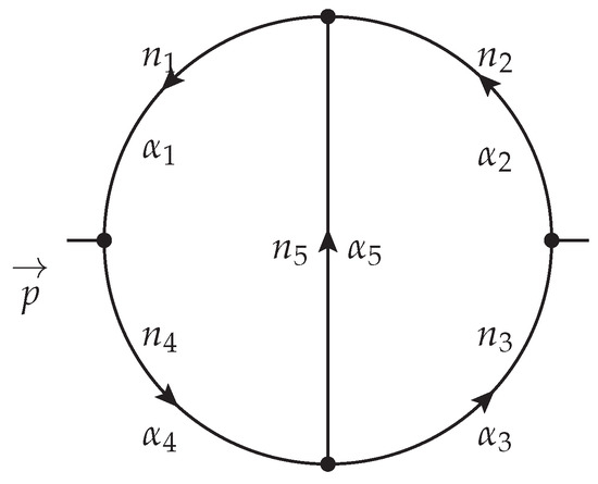
Figure 1. FI which cannot be expressed as a combination of loops and chains.

C. When $\sum {\alpha }_i=d$, there is a so-called uniqueness relation [6,7,8,9,10,11,12] for the triangle with indices ${\alpha }_i$ ($i=1,2,3$)

(12)

where

$$C_n^m=\frac{n!}{m!(n-m)!}.$$

(13)

Results (12) can be precisely obtained as follows: perform the inversion $q_i\to 1/q_i$ $(i=1,2,3)$, $k\to 1/k$ in the integrand and in the integral measure. Inversion preserves the angles between momenta. After the inversion, one propagator disappears, because $\sum {\alpha }_i=d$, and the considered triangle turns into a loop. Calculating the loop using (8) and returning it to the original momenta, we obtain the rule (12). Its extension to the case of two TPs can be found in [22].

D. For any triangle with indices ${\alpha }_i$ ($i=1,2,3$), there is the following relation based on the IBP procedure [7,19,87] (for non-zero n, m, and k values, Equation (14) was obtained in Refs. [20,21,22].)

(14)

The result (14) can been obtained by introducing the factor $(\partial /\partial k_{\mu }){(k-q_1)}^{\mu }=d$ to the integrand of the triangle, shown below as $[\dots ]$, and using the IBP procedure as follows:

$$\begin{array}{ccc}& & d\int Dk\left[\dots \right]=\int Dk\left(\frac{\partial }{\partial k_{\mu }}{(k-q_1)}^{\mu }\right)\left[\dots \right]=\int Dk\frac{\partial }{\partial k_{\mu }}\left({(k-q_1)}^{\mu }\left[\dots \right]\right)\hfill \\ & & -\int Dk{(k-q_1)}^{\mu }\frac{\partial }{\partial k_{\mu }}\left(\left[\dots \right]\right)\hfill \end{array}$$

(15)

The first term in the r.h.s. is zero, because it can be represented as a surface integral on an infinite surface. By calculating the second term in the r.h.s., we reproduce Equation (14).

As can be seen from Equations (14) and (15), the line with the index ${\alpha }_1$ is distinguished. The dependence on the indexes of the other line is the same. So, we will call the line with the index ${\alpha }_1$ as the “distinguished line”. It is clear that the different selection of the distinguished line in the triangles of a diagram leads to different types of IBP relations.

Using the IBP relation (14) allows someone to change FI indexes by an integer. FI indexes can also be changed using a transformation group [7,88,89] with the elements:

(a)

Transition to a coordinate representation;

(b)

Conformal inversion transformation $p\to p^{\prime }=p/p^2$;

(c)

A special series of transformations that allows someone to make one of the vertices unique, and then apply the relation (12) to it.

The extension of the transformation group for diagrams with a TP can be found in Ref. [22].

3. Basic Massless Two-Loop FIs

The general topology of the two-loop two-point FI, which cannot be expressed as a combinations of loops and chains, is shown in Figure 1.

Below, we will mainly focus on two special cases of the FI shown in Figure 1, for ${\alpha }_3+n_3=\alpha$, $n_3=n$, ${\alpha }_j(j\ne 3)=1$, $n_j(j\ne 3)=0$ (denote by $I_1(\alpha ,n)$) and for ${\alpha }_5+n_5=\alpha$, $n_5=n$, ${\alpha }_j(j\ne 5)=1$, $n_j(j\ne 5)=0$ (denote by $I_2(\alpha ,n)$)

(16)

We will calculate the diagrams $I_1(\alpha ,n)$ and $I_2(\alpha ,n)$ using FRs similar to those obtained [13,90]. (such FRs were obtained in [13,90] by applying IBP relations to various highlighted lines.) This greatly reduces the amount of calculations.

Repeating the analysis performed in [13], we obtain the following FRs:

$$\begin{array}{ccc}& & I_1(\alpha ,n)=\frac{1}{q^2}{I}_1(\alpha -1,n)-\frac{1}{2\epsilon }\left(2I_{1,1}(\alpha ,n)+I_{2,1}(\alpha ,n)\right)\hfill \end{array}$$

(17)

$$\begin{array}{ccc}& & I_2(\alpha ,n)=\frac{2}{n+d-2-2\alpha }{I}_{2,1}(\alpha ,n)-\frac{n+2d-4-2\alpha }{n+d-2-2\alpha }\frac{1}{q^2}{I}_2(\alpha -1,n),\hfill \end{array}$$

(18)

where the inhomogeneous terms are

(19)

(20)

It can be seen that the inhomogeneous terms in the FRs (17) and (18), i.e., $I_{11}(\alpha ,n)$ and $I_{21}(\alpha ,n)$, are combinations of loops and chains, and thus, they are calculated according to the rules (4) and (8).

We note that, for massless two-point FIs, the subject of the study is the so-called coefficient functions, i.e., $C_i(\alpha ,n)$ and $C_{i,1}(\alpha ,n)$ $(i=1,2)$ for the diagrams under consideration $I_i(\alpha ,n)$ and $I_{i,1}(\alpha ,n)$ can be represented as follows

$$I_i(\alpha ,n)=N_d{C}_i(\alpha ,n)\frac{q^{{\mu }_1{\mu }_2{\mu }_3\dots {\mu }_n}}{q^{2(\alpha +2\epsilon )}},I_{i,1}(\alpha ,n)=N_d{C}_{i,1}(\alpha ,n)\frac{q^{{\mu }_1{\mu }_2{\mu }_3\dots {\mu }_n}}{q^{2(\alpha +2\epsilon )}}.$$

(21)

The result (21) corresponds to the fact that we are considering two-loop FIs. In general, the L-loop FI $I_L({\alpha }_1,{\alpha }_2,{\alpha }_3,\dots ,{\alpha }_N,n)$ containing propagators with indices ${\alpha }_i$ $(i=1,2,3,\dots ,N)$ and one TP of momenta, can be represented as

$$I_L({\alpha }_1,{\alpha }_2,{\alpha }_3,\dots ,{\alpha }_N,n)=N_d{C}_L({\alpha }_1,{\alpha }_2,{\alpha }_3,\dots ,{\alpha }_N,n)\frac{q^{{\mu }_1{\mu }_2{\mu }_3\dots {\mu }_n}}{q^{2(\overline{\alpha }-d/2\ast \left(L\epsilon \right))}}.$$

(22)

where $\overline{\alpha }={\sum }_1^N{\alpha }_i$.

The coefficient functions $C_i(\alpha ,n)$ and $C_{i,1}(\alpha ,n)$ can be directly found from the rules (4) and (8). They have the form:

$$\begin{array}{ccc}& & C_{1,1}(\alpha ,n)=A(2,1)\left(A^{0,n}(1,\alpha )-A^{0,n}(1,\alpha +\epsilon )\right),\hfill \end{array}$$

(23)

$$\begin{array}{ccc}& & C_{2,1}(\alpha ,n)=A^{0,n}(2,\alpha -1)A^{0,n}(1,\alpha +\epsilon )-A^{0,n}(1,\alpha )A^{0,n}(2,\alpha +\epsilon ),\hfill \end{array}$$

(24)

where

$$A({\alpha }_1,{\alpha }_2)=A^{0,0}({\alpha }_1,{\alpha }_2).$$

(25)

and the result for $A^{n,m}({\alpha }_1,{\alpha }_2)$ is shown in Equation (7). Thus, the coefficient functions $C_{i,1}(\alpha ,n)$ and $C_{i,1}(\alpha ,n)$ $(i=1,2)$ are represented as combinations of $\mathsf{\Gamma }$-functions.

3.1. $I_1(0,n)$ and $I_2(0,n)$

The FIs $I_1(0,n)$ and $I_2(0,n)$ can be considered boundary conditions for the FRs (17) and (18). Moreover, in a sense, they can be obtained using Equations (4) and (8) but with the additional resummation.

Indeed, expanding in the cases of $I_1(0,n)$ and $I_2(0,n)$, the corresponding momentum products as follows:

$$\begin{array}{c}\hfill \prod _{i=1}^n{(q-k_2)}^{{\mu }_i}=\sum _{k=0}^n{C}_n^k{(-1)}^k\prod _{i=1}^k{k}_2^{{\mu }_i}\prod _{j=1}^{n-k}{q}^{{\mu }_j}\mathrm{for} I_1(0,n),\end{array}$$

(26)

$$\begin{array}{c}\hfill \prod _{i=1}^n{(k_1-k_2)}^{{\mu }_i}=\sum _{k=0}^n{C}_n^k{(-1)}^k\prod _{i=1}^k{k}_2^{{\mu }_i}\prod _{j=1}^{n-k}{k}_1^{{\mu }_j}\mathrm{for} I_2(0,n),\end{array}$$

(27)

we found the results of $I_1(0,n)$ and $I_2(0,n)$ which can be represented as

$$\begin{array}{ccc}& & I_1(0,n)=\sum _{k=0}^n{C}_n^k{(-1)}^k\prod _{j=1}^{n-k}{q}^{{\mu }_j}{\overline{I}}_1(0,k)\hfill \end{array}$$

(28)

$$\begin{array}{ccc}& & I_2(0,n)=\sum _{k=0}^n{C}_n^k{(-1)}^k{\overline{I}}_2(n-k,k)\hfill \end{array}$$

(29)

where

(30)

Thus, the FIs $I_1(0,n)$ and $I_2(0,n)$ are combinations of loops and chains, and thus their coefficient functions can be found using the rules (4) and (8). So, we have for $C_1(0,n)$ and $C_2(0,n)$:

$$\begin{array}{c}\hfill C_1(0,n)=\sum _{k=0}^n{C}_n^k{(-1)}^k{A}^{0,k}(1,1)A^{0,k}(1,1+\epsilon ),\end{array}$$

(31)

$$\begin{array}{c}\hfill C_2(0,n)=\sum _{k=0}^n{C}_n^k{(-1)}^k{A}^{0,k}(1,1)A^{0,n-k}(1,1).\end{array}$$

(32)

As noted at the beginning of Section 3.1, the results for $C_i(0,n)$ ($i=1,2$) are very important for obtaining the results of $C_i(m,n)$ for any m values using Equations (17) and (18) for $\alpha =m$. However, to calculate $C_i(0,n)$, the additional summation must be performed (see Equations (31) and (32)), the exact calculation of which can be found in [63]. Here, we only present the final results for $C_i(0,n)$ ($i=1,2$):

$$\begin{array}{c}2n{C}_1(0,n-1)={\widehat{N}}_2[\frac{1}{{\epsilon }^2}{S}_1\left(n\right)+\frac{1}{2\epsilon }\left(3S_1^2\left(n\right)+7S_2\left(n\right)\right)\hfill \\ +\frac{7}{6}{S}_1^3\left(n\right)+\frac{19}{2}{S}_1\left(n\right)S_2\left(n\right)+\frac{37}{3}{S}_3\left(n\right)-4S_{2,1}\left(n\right)],\hfill \end{array}$$

(33)

$$\begin{array}{c}n(n+1)C_2(0,n-1)=(1-{(-1)}^n){\widehat{N}}_1[\frac{1}{{\epsilon }^2}+\frac{2}{\epsilon }\left(S_1\left(n\right)+\frac{1}{n+1}\right)\hfill \\ +2S_1^2\left(n\right)+4S_2\left(n\right)+2S_{-2}\left(n\right)+8\frac{S_1\left(n\right)}{n+1}+\frac{16}{{(n+1)}^2}].\hfill \end{array}$$

(34)

where

$$S_{\pm i}\left(n\right)=\sum _{m=1}^n\frac{{(\pm 1)}^m}{m^i},S_{\pm i,j}\left(n\right)=\sum _{m=1}^n\frac{{(\pm 1)}^m}{m^i}{S}_{\pm j}\left(m\right),$$

(35)

$\zeta \left(n\right)=S_n(\infty )$—Euler zeta-function and $N_1$ and $N_2$ are normalization factors.

The factor $N_2$ is

$${\widehat{N}}_2={\mathsf{\Gamma }}^2(1+\epsilon )K_1{K}_2,K_1=\frac{{\mathsf{\Gamma }}^2(1-\epsilon )}{\mathsf{\Gamma }(1-2\epsilon )},K_2=\frac{\mathsf{\Gamma }(1-\epsilon )\mathsf{\Gamma }(1-2\epsilon )\mathsf{\Gamma }(1+2\epsilon )}{{\mathsf{\Gamma }}^2(1+\epsilon )\mathsf{\Gamma }(1-3\epsilon )}$$

(36)

Since $K_2/K_1\sim O\left({\epsilon }^3\right)$, it can be replaced by the factor ${\widehat{N}}_1$

$${\widehat{N}}_1={\mathsf{\Gamma }}^2(1+\epsilon )K_1^2.$$

(37)

It is possible to add the factor ${\widehat{N}}_1$ to the definition of ${\mu }_g^2$-scale of g-scheme [91], which is related with the usual $\overline{MS}$ one as ${\mu }_g^2=K_1{\mu }_{\overline{MS}}^2$ (see discussions in Ref. [92]).

3.2. $I_1(1,n)$ and $I_2(1,n)$

Now, we calculate the cases $I_1(1,n)$ and $I_2(1,n)$, which are very important for future studies. Indeed, we see that the FIs are finite and the corresponding $C_{j,1}(1,n)$ $(j=1,2)$ have very compact form. Indeed,

$$\begin{array}{ccc}& & C_{1,1}(1,n)=-\frac{1}{2{\epsilon }^2}\left[2{\widehat{N}}_1\frac{B(n+1,-1,-2)}{n+1-2\epsilon }-{\widehat{N}}_2\frac{B(n+1,-2,-3)}{n+1-3\epsilon }\right],\hfill \end{array}$$

(38)

$$\begin{array}{ccc}& & C_{2,1}(1,n)=-\frac{{\widehat{N}}_2}{2{\epsilon }^2}\frac{B(n+1,-1,-3)}{n+1-2\epsilon },\hfill \end{array}$$

(39)

where

$$B(n+1,a_1,a_2)=\frac{\mathsf{\Gamma }(n+1+a_1\epsilon )\mathsf{\Gamma }(1+a_2\epsilon )}{\mathsf{\Gamma }(1+a_1\epsilon )\mathsf{\Gamma }(n+1+a_2\epsilon )}.$$

(40)

Expanding $\mathsf{\Gamma }$-functions as

$$\begin{array}{ccc}& & \frac{\mathsf{\Gamma }(n+1+a\epsilon )}{n!\mathsf{\Gamma }(1+a\epsilon )}=exp\left[-\sum _{m=1}^{\infty }\frac{{(-a\epsilon )}^m}{m}{S}_m\left(n\right)\right],\hfill \end{array}$$

(41)

$$\begin{array}{ccc}& & \mathsf{\Gamma }(1+a\epsilon )=exp\left[-\gamma a\epsilon +\sum _{m=1}^{\infty }\frac{{(-a\epsilon )}^m}{m}{\zeta }_m\right],\hfill \end{array}$$

(42)

with the Euler’s constant $\gamma$, we obtain ($a_{\pm }=a_1\pm a_2)$)

$$\begin{array}{c}\hfill \begin{array}{ccc}& & \hfill B(n+1,a_1,a_2)=exp\left[-\sum _{m=1}^{\infty }\frac{{(-\epsilon )}^m}{m}\left[a_1^m-a_2^m\right]S_m\left(n\right)\right]=1+a_{-}\epsilon S_1\left(n\right)+\frac{{\epsilon }^2}{2}\left[a_{-}^2{S}_1^2\left(n\right)-a_{-}{a}_{+}{S}_2\left(n\right)\right]\\ & & \hfill +\frac{{\epsilon }^3}{3!}\left[a_{-}^3{S}_1^3\left(n\right)-3a_{-}^2{a}_{+}{S}_1\left(n\right)S_2\left(n\right)+2(a_1^3-a_2^3)S_3\left(n\right)\right]+O\left({\epsilon }^4\right).\end{array}\end{array}$$

(43)

With the evaluation of the results (38) and (39), we see that all singularities are canceled and the final results are (${\delta }_n^m$ for the Kronecker symbol: ${\delta }_n^n=1$ and ${\delta }_n^m=0$ for $n\ne m$)

$$\begin{array}{ccc}& & (n+1)C_1(1,n)=S_3\left(n\right)+S_1\left(n\right)S_2\left(n\right)-S_{2,1}\left(n\right)+6{\zeta }_3+O\left(\epsilon \right),\hfill \end{array}$$

(44)

$$\begin{array}{ccc}& & (n+1)C_2(1,n)=(1+{(-1)}^n)\left(3{\delta }_n^0{\zeta }_3-(1-{\delta }_n^0)\frac{2S_{-2}\left(n\right)}{n}\right)+O\left(\epsilon \right),\hfill \end{array}$$

(45)

where we use the condition $C_1(1,n=0)=6{\zeta }_3$, since $C_2(1,n=0)=C_1(1,n=0)$. (The result $C_1(1,n=0)=6{\zeta }_3$ can be directly obtained from Equation (45) using an analytic continuation of $S_{-2}\left(n\right)$ (see Appendix A)).

The results (44) and (45) are the real example of the coefficient functions in DIS structure functions (see, e.g., Refs. [78,79,93]).

4. Examples of the Calculation of Four-Point Massless FIs

In the previous Section 3, we considered the basic FIs $I_1(\alpha ,n)$ and $I_1(\alpha ,n)$ with $\alpha =0$ and $\alpha =1$.

Here, we study the expansion coefficients of scalar FIs (which we call the FI “moments”), arising in the investigations of forward elastic scattering. These moments are extracted from the initial FIs with the help of the method of “projectors” [94,95,96,97], the basic properties of which are considered in Appendix B.

4.1. FIs $I_1(n+1,n)$ and $I_2(n+1,n)$

Firstly, we consider the two simplest FIs: $J_1(\alpha =1,q,p)$ and $J_2(\alpha =1,q,p)$, shown in Figure 2. As already discussed above, using the “projectors” method (see Appendix B), it is possible to introduce the so-called moments $J_i(\alpha =1,n)$ $(i=1,2)$. The moments of the FIs shown in Figure 2 are represented by the FIs in Equation (16) for $\alpha =n+1$, i.e., $J_i(\alpha =1,n)=I_i(n+1,n)$.

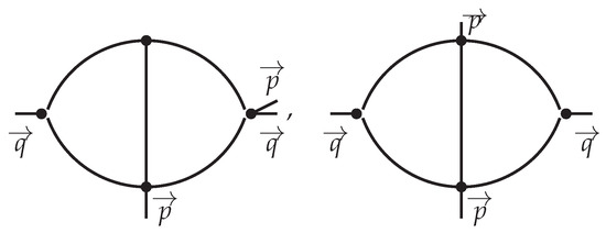
Figure 2. The simplest four-point FIs: $J_1(\alpha =1,q,p)$ and $J_2(\alpha =1,q,p)$.

To calculate the FIs, it is convenient to apply the Fourier transforms [16]

$$\begin{array}{ccc}& & \int d^{d}p{e}^{ipx}\frac{1}{p^{2\alpha }}=2^{2\tilde{\alpha }}{\pi }^{d/2}{a}_0\left(\alpha \right)\frac{1}{x^{2\tilde{\alpha }}},(\tilde{\alpha }=\frac{d}{2}-\alpha ,\mathrm{see}\mathrm{Equation}\left(7\right)),\hfill \end{array}$$

(46)

$$\begin{array}{ccc}& & \int d^{d}p{e}^{ipx}\frac{p^{{\mu }_1}{p}^{{\mu }_2}{p}^{{\mu }_3}\dots p^{{\mu }_n}}{p^{2(\alpha +n)}}={(-i)}^n{2}^{2\tilde{\alpha }}{\pi }^{d/2}{a}_n(\alpha +n)\frac{x^{{\mu }_1}{x}^{{\mu }_2}{x}^{{\mu }_3}\dots x^{{\mu }_n}}{x^{2\tilde{\alpha }}}+\dots ,\hfill \end{array}$$

(47)

where the symbol “…” marks the neglected terms of the order $g^{{\mu }_i{\mu }_j}$.

The Fourier transform (46) is the usual one (see, e.g., the recent review [16] and discussion therein) but the Fourier transform (47) can be obtained from Equation (46) using the projector ${\partial }^{{\mu }_1}/{(\partial x)}^{{\mu }_1}\dots {\partial }^{{\mu }_n}/{(\partial x)}^{{\mu }_n}$.

To show its effectiveness, it is possible to study more complex FIs $I_i(\alpha +n,n)$ $(i=1,2)$ which have coefficient functions $C_i(\alpha +n,n)$

$$I_i(\alpha +n,n)=N_d{C}_i(\alpha +n,n)\frac{q^{{\mu }_1{\mu }_2{\mu }_3\dots {\mu }_n}}{q^{2(\alpha +n+2\epsilon )}},$$

(48)

which are similar to Equation (21).

Applying the above Fourier transforms to the l.h.s., we obtain the following FIs in the x-space:

If we replace x and all internal coordinates with the momentum q and the corresponding internal momenta, we obtain equivalent diagrams in momentum space. We call them ${\overline{I}}_i(\tilde{\alpha },n)$. We call such a replacement a “dual transformation” (see discussion in [16]) and denote as $\stackrel{d}{=}$. So, we obtain

We denote the coefficient functions of the last FIs as ${\overline{C}}_i(\tilde{\alpha },n)$, i.e.,

$${\overline{I}}_i(\tilde{\alpha },n)=N_d{\overline{C}}_i(\tilde{\alpha },n)\frac{q^{{\mu }_1{\mu }_2{\mu }_3\dots {\mu }_n}}{q^{2(\tilde{\alpha }-2\epsilon )}}.$$

(49)

Performing Fourier transforms for both parts of Equation (48) (see Ref. [16]), we obtain the relations between the coefficient functions $C_i(\alpha +n,n)$ and ${\overline{C}}_i(\tilde{\alpha },n)$ in the following form:

$$C_i(\alpha +n,n)=K(\alpha +n,n){\overline{C}}_i(\tilde{\alpha },n),$$

(50)

where

$$K(\alpha +n,n)=\frac{a_0^4\left(1\right)a_n(\alpha +n)}{a_n(\alpha +n+2\epsilon )}=\frac{{\mathsf{\Gamma }}^4(1-\epsilon )\mathsf{\Gamma }\left(\tilde{\alpha }\right)\mathsf{\Gamma }(\alpha +n+2\epsilon )}{\mathsf{\Gamma }(\alpha +n)\mathsf{\Gamma }(\tilde{\alpha }-2\epsilon )}.$$

(51)

Now, we return to the case $\alpha =1$, then

$${\overline{C}}_i(1-\epsilon ,n)=C_i(1,n)+0\left({\epsilon }^0\right),K(n+1,n)=\frac{{\mathsf{\Gamma }}^5(1-\epsilon )\mathsf{\Gamma }(n+1+2\epsilon )}{n!\mathsf{\Gamma }(1-3\epsilon )}=1+0\left({\epsilon }^0\right).$$

(52)

So, we see from Equation (50) that

$$C_i(n+1,n)=C_i(1,n)+O\left(\epsilon \right).$$

(53)

i.e.,

$$\begin{array}{ccc}& & (n+1)C_1(n+1,n)=S_3\left(n\right)+S_1\left(n\right)S_2\left(n\right)-S_{2,1}\left(n\right)+6{\zeta }_3+O\left(\epsilon \right),\hfill \end{array}$$

(54)

$$\begin{array}{ccc}& & (n+1)C_2(n+1,n)=(1+{(-1)}^n)\left(3{\delta }_n^0{\zeta }_3-(1-{\delta }_n^0)\frac{2S_{-2}\left(n\right)}{n}+O\left(\epsilon \right)\right).\hfill \end{array}$$

(55)

4.2. FIs $I_1(n+2,n)$ and $I_2(n+2,n)$

Now, we consider the more complicated FIs ${\overline{J}}_1(\alpha =1,q,p)$ and ${\overline{J}}_2(\alpha =1,q,p)$ shown in Figure 3.

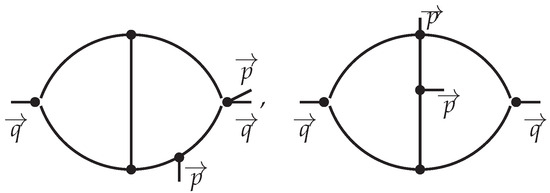
Figure 3. The FIs ${\overline{J}}_1(\alpha =1,q,p)$ and ${\overline{J}}_2(\alpha =1,q,p)$.

Their moments ${\overline{J}}_i(\alpha =1,n)$ $(i=1,2)$ are equal to the FIs in Equation (16) with $\alpha =n+2$, i.e., to $I_i(n+2,n)$. Their coefficient functions $C_i(n+2,n)$ $(i=1,2)$ can be expressed in terms of the $C_i(n+1,n)$ given in Equations (54) and (55) and $C_{i1}(n+2,n)$ given in Equations (23) and (24) with $\alpha =n+2$.

Performing calculations, we obtain $C_{11}(1,n)$ and $C_{21}(1,n)$ in the following form

$$\begin{array}{ccc}& & \frac{C_{11}(n+2,n)}{1/\left(2{\epsilon }^2\right)}=2{\widehat{N}}_1\frac{B(n+1,1,0)}{n+1}-{\widehat{N}}_2\frac{B(n+1,2,1)}{n+1+\epsilon }=2{\widehat{N}}_1\frac{B(n+2,1,0)}{n+1+\epsilon }-{\widehat{N}}_2\frac{B(n+2,2,1)}{n+1+2\epsilon },\hfill \end{array}$$

(56)

$$\begin{array}{ccc}& & \frac{C_{2,1}(n+2,n)}{{\widehat{N}}_2/\left(2{\epsilon }^2\right)}=\frac{B(n+1,1,0)}{n+1+\epsilon }B(n+1,2,1)-3\frac{B(n+1,1,0)}{n+1}B(n+2,2,1),\hfill \end{array}$$

(57)

where the normalizations ${\widehat{N}}_1$ and ${\widehat{N}}_2$ and the factors $K_1$ and $K_2$ are given in Equations (37) and (36), respectively.

Evaluating the r.h.s. of Equations (56) and (57), after some algebra, we have obtain the final results as

$$\begin{array}{c}n\frac{C_1(n+1,n-1)}{{\widehat{N}}_2}=\frac{1}{2{\epsilon }^2}{S}_1\left(n\right)+\frac{1}{4\epsilon }\left[3S_1^2\left(n\right)-5S_2\left(n\right)\right]+\frac{7}{12}{S}_1^3\left(n\right)\hfill \\ -\frac{5}{4}{S}_1\left(n\right)S_2\left(n\right)+\frac{19}{6}{S}_3\left(n\right)-2S_{2,1}\left(n\right)-\frac{S_1\left(n\right)}{n^2},\hfill \end{array}$$

(58)

$$\begin{array}{c}n(n+1)\frac{C_2(n+1,n-1)}{{\widehat{N}}_2}=(1-{(-1)}^n)(\frac{1}{{\epsilon }^2}+\frac{2}{\epsilon }\left[S_1\left(n\right)-\frac{1}{n+1}\right]\hfill \\ +2S_1^2\left(n\right)-2S_2\left(n\right)-4\frac{S_1\left(n\right)}{n+1}+\frac{1}{{(n+1)}^2}),\hfill \end{array}$$

(59)

where we added the extra factor $(1-{(-1)}^n)/2$ to the coefficient function $C_2(n+1,n-1)$. The demonstration of even more complicated examples can be seen in Refs. [20,21,22].

We note that, for FIs containing several propagators depending on the momentum p (see, e.g., ${\widehat{J}}_1(\alpha ,\beta ,q,p)$ in Appendix B), their moments contain the sum of two-point FIs (see, for example, the moment ${\widehat{J}}_1(\alpha ,\beta ,n)$ in Appendix B). Calculating the moments of such a type is a much more difficult task than $I_i(n+1,n)$ and $I_i(n+2,n)$ with the $(i=1,2)$ considered above. However, as it was shown in Ref. [22], it is almost always possible to split in the contributions the complicated integrals and complicated series. Moreover, $\epsilon$-singularities are only contained in the simplest parts, which can usually be summed up in all orders in $\epsilon$.

5. ${\mathit{kR}}^{\prime }$-Operation

The calculation of massless FIs is the most important procedure for calculating the critical parameters of models and theories, such as the anomalous dimensions of fields and operators, as well as $\beta$-functions. One of the most convenient calculation recipes is that of the Bogolyubov–Parasyuk–Hepp–Zimmerman (BPHZ) R-operation [98,99,100], which sequentially extracts all FI singularities. Formally, it has the following form

$$R\left[FI\right]=FI-k{R}^{\prime }\left[FI\right],$$

(60)

where $k{R}^{\prime }$ is the operation that takes into account all the singularities of the FI subgraphs, with the exception of the singularities of the FI itself. The very important property of the $k{R}^{\prime }$-operation is the independence of the results of its application from the external momenta and masses. The independence is the basis of the so-called infra-red rearrangement approach [101] (as can also be seen in Refs. [102,103,104]), which gives a possibility to only study FIs with the minimum possible set of masses and external momenta. We note that such neglecting masses and momenta should not lead to an appearance of infrared singularities. The possibility to delete and modify external momenta is widely used (see, e.g., [105] and the discussions therein). We will try to show this in our examples below, where we take a detailed look at the computation of singular structures up to five-loop FIs that contribute to the $\beta$-function of the ${\phi }^4$ model.

To demonstrate the opportunities of the $k{R}^{\prime }$-operation, it is useful to start with one-loop and two-loop FIs.

One loop. Putting ${\alpha }_1={\alpha }_2=1$ in Equation (8), we obtain

(61)

where $N_d$ is given in Equation (6) and $\overline{\mu }$ is the renormalization scale in the $\overline{MS}$-scheme, defined as

$${\overline{\mu }}^{2\epsilon }={\mu }^{2\epsilon }{\left(4\pi \right)}^{\epsilon }\mathsf{\Gamma }(1+\epsilon ).$$

(62)

By definition, $k{R}^{\prime }$ is an operation, which is equal to k-operation in the one-loop case, since there are no subgraphs, i.e.,

(63)

which, of course, does not depend on $q^2$.

Two loops. Now, we consider the following FI

(64)

As already mentioned, the $R^{\prime }$-operation extracts the singularities of subgraphs. In the case under consideration, we have a singular inner loop, the singularity of which is shown above in Equation (63). Thus, the $R^{\prime }$-operation of the considered two-loop FI has the form

(65)

Evaluating diagrams in the r.h.s. and taking their singular parts (by the k-operation), we obtain

(66)

where

$$L=ln\left(\frac{{\overline{\mu }}^2}{q^2}\right).$$

(67)

As we can see, the result is $q^2$-independent, which is due to the local renormalization properties.

Three and four loops. To find three- and four-loop corrections to the $\beta$-function of the ${\phi }^4$ model, it is necessary, in particular, to calculate the singular parts of the following vertex FIs:

(68)

For the first diagram, we have

(69)

where we used the result $C_2(n+1,n)$ in Equation (55) for $n=0$.

We note that, for ${\alpha }_i=1+a_i\epsilon$, there is the following result (beyond $O\left({\epsilon }^2\right)$, the coefficients of the expansion can be found in [15,90].).

(70)

where

$$\begin{array}{c}{\widehat{N}}_d=N_d\mathsf{\Gamma }(1+\epsilon ),a={\sum }_{i=1}^5{a}_i,A_{2,1}=30{\overline{A}}_1+45a_5,{\overline{A}}_n={\sum }_{i=1}^4{a}_i^n,\hfill \\ \\ A_{2,2}=10{\overline{A}}_2+45a_5^2+15{\overline{A}}_1{a}_5+10\left(a_1{a}_2+a_3{a}_4+a_1{a}_4+a_2{a}_3\right)+5\left(a_1{a}_3+a_2{a}_4\right).\hfill \end{array}$$

(71)

The result (70) was obtained using the IBP relation (14) and transformation rules (see, e.g., [15] and the references therein). Indeed, for the case ${\alpha }_2={\alpha }_4={\alpha }_5=1$, we have from Equation (14)

(72)

For the second diagram in (68), we have

(73)

since the singularity does not depend on the external momenta. So, we have

(74)

because

(75)

The result (75) can be obtained as follows. Using the IBP relation for an interior triangle with the distinguished line between the top interior points, we have

(76)

Using other IBP relations and transformation rules (see, e.g., [15] and references therein), a more accurate result can be obtained for ${\alpha }_i=1+a_i$ $(i=1,2,3,\dots ,7)$

(77)

where $a_{4567}={\sum }_{i=4}^7{a}_i$ and $a={\sum }_{i=1}^7{a}_i$.

Five Loop Corrections in the ${\phi }^4$ Model

We apply the method described above to the calculation of five-loop singularities in the ${\phi }^4$ model. In this regard, let us recall that the five-loop corrections to anomalous dimensions and the $\beta$-function in this model in the scheme $\overline{MS}$ were calculated a long time ago in [30]. For a complete calculation, it was necessary to calculate about 120 diagrams. The results for all but four were analytically found using the IBP procedure. For the four most complex diagrams, the application of the decomposition of one of the propagators into Gegenbauer polynomials led to results in the form of a triple infinite convergent series. The computer summation of the series allowed the authors to achieve good accuracy. However, it was desirable to obtain an analytic assessment of these contributions, which was performed by Kazakov (see Refs. [13,90]). To show the possibilities of the methods discussed above, we present the calculation of two of these complex FIs, which have the following form

(78)

First FI. Calculating the first FI with an accuracy of $O\left({\epsilon }^{-1}\right)$ is equal to calculating the diagram

(79)

with an accuracy of $O\left(\epsilon \right)$. Using the IBP procedure to the left triangle with the vertical distinguished line, we have the following relation:

(80)

The first diagram in the r.h.s. is the product of one-loop and two-lop FIs that are already considered above. To evaluate the second diagram, the IBP procedure is applied to the left triangle with the upper distinguished line to the diagram in Equation (75). We have

(81)

Taking this equation together with Equation (76), we obtain the following

(82)

Then, plugging this result into the r.h.s. of Equation (80) and calculating the one-loop diagram, we have for the r.h.s.:

(83)

Evaluating these two-loop master integrals using the result provided by Equation (70), we obtain the results of the FI in Equation (79) with the accuracy $O\left({\epsilon }^2\right)$:

(84)

Taking into account the two additional loops, we have the additional factor:

$$A(1,2+3\epsilon )A(1,1+4\epsilon )=-\frac{N_d^2}{20{\epsilon }^2}\frac{1}{(1+3\epsilon )(1-6\epsilon )}\frac{{\mathsf{\Gamma }}^2(1-\epsilon )\mathsf{\Gamma }(1-4\epsilon )\mathsf{\Gamma }(1+6\epsilon )}{\mathsf{\Gamma }(1+3\epsilon )\mathsf{\Gamma }(1-6\epsilon )}.$$

(85)

So, the final result for the first FI in Equation (78) has the form:

(86)

Second FI. Now, consider the second FI in Equation (78). The $k{R}^{\prime }$-operation of the diagram has the following form

(87)

which contains the FI itself and its counter-term containing the inner-loop singularity.

Since the r.h.s. should be $q^2$-independent, the external momenta can be canceled and inserted into points A and B:

(88)

The r.h.s. now looks like this

(89)

where integrals $I_4$ and $I_3$ are internal blocks forming the FIs in r.h.s. of Equation (88) after integrating these blocks with the propagator connecting points A and B. Due to dimensional properties, integrals $I_4$ and $I_3$ should have the form

(90)

where $C_4$ and $C_3$ are the coefficient functions of the $I_4$ and $I_3$ integrals.

So, we have that

(91)

where all $q^2$-dependence is canceled in the r.h.s. singularities.

For FIs similar to the diagrams in r.h.s. of Equation (88), but with the index $1-\epsilon$ on the line between A and B, we have the following

(92)

We would like to note that, in the l.h.s., we can extract the line between points A and C, as an external line; then, we have

(93)

and, thus,

(94)

where $C_{4,1}$ and $C_{3,1}$ are the coefficient functions of the integrals $I_{4,1}$ and $I_{3,1}$, which are internal blocks that create FIs in the r.h.s. of Equation (93) after integrating these blocks with the propagator between points A and C. Due to the dimension properties, the $I_{4,1}$ and $I_{3,1}$ integrals can be represented in the form

(95)

because both $I_{4,1}$ and $I_{3,1}$ contain one line with the index $1-\epsilon$.

Now, consider an FI similar to the original one, but with lines between points A and B and points A and C having indexes $1-\epsilon$. Taking, as stated above, the line between points A and C as the outer one, we obtain the results

(96)

Now, we can represent the l.h.s. FI as blocks containing two lines with the index $1-\epsilon$ and some additional lines between D and E:

(97)

where $C_{4,2}$ and $C_{3,2}$ are the coefficient functions of integrals $I_{4,2}$ and $I_{3,2}$, which can be obtained from r.h.s. FIs by removing the line between D and E. Since $I_{4,2}$ and $I_{3,2}$ have two lines with index $1-\epsilon$, from the dimension properties, they can be represented as

(98)

Now, consider the FI $I_{4.2}$. Integrating the inner loop, we obtain the following

(99)

The DAC vertex in the r.h.s. FI is a unique vertex and therefore can be replaced by the corresponding triangle, as shown in Equation (12). So, we see that

(100)

Now, the triangle CBE in the r.h.s. FI is uniquetriangle and therefore can be replaced by the corresponding vertex according to the rule (12):

(101)

So, finally we obtain

(102)

where the integral $J_1^{\left(1\right)}$ is table one (see Ref. [16]) (note that the results obtained in [16] are a simple recalculation of the previously obtained x-space results [8,9,10,11,12,13]. It is convenient to use the concept of so-called dual diagrams for recalculation (see, for example, Refs. [20,21,22] and the discussion in Section 4.1), which were obtained from the original FIs by replacing all momenta with coordinates. With such a replacement, the results themselves remain unchanged, only their graphical representation changes. As a rule, dual diagrams are used in the massless case (as can be seen in [20,21,22]), but sometimes they are also used for FIs with massive propagators (see, for example, [28,29,106])): $J_1^{\left(1\right)}=J_1(1,1,1,1,1,1-\epsilon ,1-\epsilon )$. Here,

(103)

where $a={\sum }_{k=1}^7{a}_i$, $a_{4567}={\sum }_{k=4}^7{a}_i$ and

$$C_1(a_1,a_2,a_3,a_4,a_5,a_6,a_7)=\frac{1}{1-2\epsilon }\left[20{\zeta }_5+\left(50{\zeta }_6+\left(20+a_{4567}\right){\zeta }_3^3\right)\epsilon +O\left({\epsilon }^2\right)\right].$$

(104)

By entering short notations $C_1^{\left(1\right)}=C_1(1,1,1,1,1,1-\epsilon ,1-\epsilon )$ and $C_1^{\left(0\right)}=C_1(1,1,1,1,1,1,1)$, it is convenient to write the following:

$$C_1^{\left(1\right)}=C_1^{\left(0\right)}\left(1+\frac{3{\zeta }_3^2}{10{\zeta }_5}\epsilon \right),$$

(105)

where

$$C_1^{\left(0\right)}=\frac{10}{1-2\epsilon }\left[2{\zeta }_5+\left(5{\zeta }_6+2{\zeta }_3^3\right)\epsilon +O\left({\epsilon }^2\right)\right]$$

(106)

The counter-terms $I_3\left(q^2\right)$, $I_{3,1}\left(q^2\right)$ and $I_{3,2}\left(q^2\right)$ can also be expressed through $J_1(a_1,a_2,a_3,a_4,a_5,a_6,a_7)$ in the form:

$$I_{3,2}\left(q^2\right)=J_1(1,1-\epsilon ,1-\epsilon ,1,1,1,1),I_{3,1}\left(q^2\right)=J_1(1-\epsilon ,1,1,1,1,1,1),I_3\left(q^2\right)=J_1(1,1,1,1,1,1,1).$$

(107)

So, within the accuracy $O\left({\epsilon }^2\right)$, their coefficient functions exactly coincide:

$$C_3=C_{3,1}+O\left({\epsilon }^2\right)=C_{3,2}+O\left({\epsilon }^2\right)=C_1^{\left(0\right)}+O\left({\epsilon }^2\right).$$

(108)

Taking into account the above relations and the one-loop results $A(\alpha ,\beta )$, it can be shown that with an accuracy of $O\left({\epsilon }^2\right)$, the results for the four-loop coefficient functions are also the same. Indeed, we obtain

$$\begin{array}{ccc}& & C_{4,1}=C_{4,2}\frac{A(1,1+2\epsilon )}{A(1-\epsilon ,1+3\epsilon )}-\frac{C_{3,1}}{\epsilon }\frac{e^{(-L\epsilon )}}{A(1-\epsilon ,1+3\epsilon )}\left[A(1,1+\epsilon )-A(1-\epsilon ,1+2\epsilon )\right]+O\left({\epsilon }^2\right),\hfill \\ & & C_4=C_{4,1}\frac{A(1,1+3\epsilon )}{A(1-\epsilon ,1+4\epsilon )}-\frac{C_3}{\epsilon }\frac{e^{(-L\epsilon )}}{A(1-\epsilon ,1+4\epsilon )}\left[A(1,1+2\epsilon )-A(1-\epsilon ,1+3\epsilon )\right]+O\left({\epsilon }^2\right).\hfill \end{array}$$

The terms $\sim C_{3,1}$ and $\sim C_3$ are suppressed and we obtain the following

$$C_4=C_{4,1}+O\left({\epsilon }^2\right)=C_{4,2}+O\left({\epsilon }^2\right)$$

(109)

and, thus,

$$C_4=C_1^{\left(1\right)}+O\left({\epsilon }^2\right)=C_1^{\left(0\right)}\left(1+\frac{3{\zeta }_3^2}{10{\zeta }_5}\epsilon \right)+O\left({\epsilon }^2\right).$$

(110)

So, the results for initial diagrams, as shown in the r.h.s. of Equation (87), using the r.h.s. of Equation (91), can be represented as

(111)

and

(112)

So, for the second diagram in Equation (78), we have

(113)

where the definition of L is presented in Equation (67). Taking into account the results for $C_1^{\left(1\right)}$ and $C_1^{\left(0\right)}$, given in Equations (105) and (106), respectively, we obtain the final following result:

(114)

The reception of this result came a long way; however, all steps are absolutely transparent. Moreover, a similar approach can be used to evaluate other FIs.

6. Calculation of Massive FIs

FIs with massive propagators are significantly more complicated objects compared to massless FIs. The basic rules for FI calculating, as already discussed in Section 2, should be supplemented with new rules containing directly massive propagators. These additional rules will be introduced now.

A propagator with the index $\alpha$ and mass M is graphically represented as

(115)

The following useful formulas exist.

A. The product of propagators with indices ${\alpha }_1$ and ${\alpha }_2$ and with the same mass M (i.e., the chain of two massive propagators with the same mass) is equivalent to a new propagator with index $\alpha ={\alpha }_1+{\alpha }_2$ and mass M:

$$\frac{1}{{(q^2+M^2)}^{{\alpha }_1}}\frac{1}{{(q^2+M^2)}^{{\alpha }_2}}=\frac{1}{{(q^2+M^2)}^{({\alpha }_1+{\alpha }_2)}},$$

or graphically

(116)

B. Massive tadpole is exactly integrated:

$$\int \frac{Dk}{k^{2{\alpha }_1}{(k^2+M^2)}^{{\alpha }_2}}=N_d\frac{R({\alpha }_1,{\alpha }_2)}{M^{2({\alpha }_1+{\alpha }_2-d/2)}}$$

where

$$R(\alpha ,\beta )=\frac{\mathsf{\Gamma }(d/2-{\alpha }_1)\mathsf{\Gamma }({\alpha }_1+{\alpha }_2-d/2)}{\mathsf{\Gamma }(d/2)\mathsf{\Gamma }\left({\alpha }_2\right)}.$$

(117)

C. The result of calculating the FI containing two massive propagators (i.e., a loop) with masses $M_1$ and $M_2$ and indices ${\alpha }_1$ and ${\alpha }_2$ can be represented as a ${}_2{F}_1$-hypergeometric function that can be obtained in various ways, for example, by the Feynman-parameter method. However, using this approach, it is very useful to represent the loop as a one-fold integral of the new propagator with an ‘effective mass’ $\mu$ [23,24,25,26,27,62,107,108,109,110]:

$$\begin{array}{ccc}& & \times \int \frac{Dk}{{[{(q-k)}^2+M_1^2]}^{{\alpha }_1}{[k^2+M_2^2]}^{{\alpha }_2}}\hfill \\ & & =N_d\frac{\mathsf{\Gamma }({\alpha }_1+{\alpha }_2-d/2)}{\mathsf{\Gamma }\left({\alpha }_1\right)\mathsf{\Gamma }\left({\alpha }_2\right)}{\int }_0^1\frac{ds{s}^{{\alpha }_1-1}{(1-s)}^{{\alpha }_2-1}}{{[s(1-s)q^2+M_1^{2}s+M_2^2(1-s)]}^{{\alpha }_1+{\alpha }_2-d/2}}\hfill \\ & & =N_d\frac{\mathsf{\Gamma }({\alpha }_1+{\alpha }_2-d/2)}{\mathsf{\Gamma }\left({\alpha }_1\right)\mathsf{\Gamma }\left({\alpha }_2\right)}{\int }_0^1\frac{ds}{s^{1-{\tilde{\alpha }}_2}{(1-s)}^{1-{\tilde{\alpha }}_1}}\frac{1}{{[q^2+{\mu }^2]}^{{\alpha }_1+{\alpha }_2-d/2}},\left({\mu }^2=\frac{M_1^2}{1-s}+\frac{M_2^2}{s}\right).\hfill \end{array}$$

It is convenient to also rewrite the equation graphically:

(118)

D. For any triangle with masses $M_i$ ($i=1,2,3$) and indices ${\alpha }_i$, the following relation is obtained using the IBP procedure [7,19,23,24,25,26,27,87]

(119)

By analogy with the massless case (see Equation (14)), Equation (119) can be obtained by introducing the coefficient $d=(\partial /\partial k_{\mu }){(k-q_1)}^{\mu }$ to the subintegral expression of the triangle and using integration by parts as in Equation (15).

Also, similarly to the massless case, the line with the index ${\alpha }_1$ enters asymmetrically, and as a result, it is distinguished. Therefore, we will call the line with the index ${\alpha }_1$ as the “distinguished line”. It is clear that there are different relationship options with different distinguished lines leading to different types of IBP relations.

7. Two-Loop On-Shall MI

Here, we consider the two-loop on-shall MI (in this section, we use the condition $q^2=-m^2$, since Euclidean space is used)

(120)

It contributes the ${\alpha }_s$-correction to the ratio between the $\overline{MS}$ and the pole masses of the Higgs boson in the standard model.

Except in special cases, below we will not specify the masses of m and M, but rather thin and thick lines for the propagators with m and M, respectively.

Applying the IBP relation for the inner loop of the FI $I(m^2,M^2)$, we obtain

(121)

where the last integral in the r.h.s. can be represented as

$$-\frac{1}{2}\frac{\partial }{\partial M^2}I(m^2,M^2).$$

(122)

Thus, Equation (121) can be represented as the DE

$$(4M^2-m^2)\frac{1}{2}\frac{\partial }{\partial M^2}I(m^2,M^2)=(d-3)I(m^2,M^2)+J(m^2,M^2),$$

(123)

with the inhomogeneous term (IT)

(124)

which contains only substantially simpler FIs. The DE solution with the boundary condition $J(m^2,M^2\to \infty )=0$ has the following form

$$\begin{array}{ccc}& & I(M^2,m^2)=N_d^2\overline{I}\left(x\right)\frac{{\left({\overline{\mu }}^2\right)}^{2\epsilon }}{{\left(m^2\right)}^{2\epsilon }},J(M^2,m^2)=N_d^2\overline{J}\left(x\right)\frac{{\overline{\mu }}^2}{{\left(m^2\right)}^{2\epsilon }},\hfill \end{array}$$

(125)

$$\begin{array}{ccc}& & \overline{I}\left(x\right)=-{(4x-1)}^{1/2-\epsilon }{\int }_x^{\infty }\frac{2{\overline{I}}_1\left(x_1\right)d{x}_1}{{(4x_1-1)}^{3/2-\epsilon }}=-\frac{{(4-z)}^{1/2-\epsilon }}{z^{1/2-\epsilon }}{\int }_0^z\frac{2\overline{J}\left(z_1\right)d{z}_1}{z_1^{1/2+\epsilon }{(4-z_1)}^{(3/2-\epsilon )}},\hfill \end{array}$$

(126)

where

$$x=\frac{M^2}{m^2},z=\frac{M^2}{m^2}=\frac{1}{x}.$$

(127)

Applying the IBP procedure for each FI included in $J(M^2,m^2)$, we obtain similar DEs for them. Solving these DEs, we obtain the following result for $\overline{J}\left(x\right)$

$$\overline{J}\left(z\right)=\left[-\frac{1}{2{\epsilon }^2}+\left(a_1-\frac{3}{2}\right)\frac{1}{\epsilon }+a_2+2a_1-\frac{9}{2}+a_{1}lnz+\frac{1-z}{z}{\overline{\mathrm{Li}}}_2\left(z\right)+\frac{1}{2}{ln}^{2}z\right],$$

(128)

where

$$a_1=-\frac{\pi }{\sqrt{3}},a_2=\frac{4}{\sqrt{3}}{\mathrm{Cl}}_2\left(\frac{\pi }{3}\right)-\frac{\pi }{\sqrt{3}}ln3,{\overline{\mathrm{Li}}}_2\left(z\right)={\mathrm{Li}}_2\left(z\right)+lnzln(1-z)$$

(129)

and ${\mathrm{Li}}_2\left(z\right)$ is the dilogarithm [111] (for more complicated functions, see Ref. [112]).

$\overline{I}\left(x\right)$

To calculate the FI $\overline{I}\left(x\right)$, we need to calculate several integrals. The first integral, which contains the x-independent part of $\overline{J}\left(x\right)$, is simple:

$${\overline{I}}_1\left(x\right)={(4x-1)}^{1/2-\epsilon }{\int }_x^{\infty }\frac{d{x}_1}{{(4x_1-1)}^{3/2-\epsilon }}=\frac{1}{2(1-2\epsilon )}.$$

(130)

The remaining integrals will be calculated up to $\epsilon =0$.

The integral $\sim lnz$ in $\overline{J}\left(x\right)$ is convenient to calculate using the IBP procedure (the IBP procedure was used in a similar way for integral representations in a recent paper [113], where FIs containing elliptic structures were considered). how

$${\overline{I}}_2\left(x\right)={(4x-1)}^{1/2}{\int }_x^{\infty }\frac{d{x}_1}{{(4x_1-1)}^{3/2}}ln\left(\frac{1}{x_1}\right)=\frac{1}{2}\left[ln\left(\frac{1}{x}\right)-\tilde{I}\left(x\right)\right],$$

(131)

where (see Appendix C)

$$\begin{array}{ccc}& & \tilde{I}\left(x\right)={(4x-1)}^{1/2}{\int }_x^{\infty }\frac{d{x}_1}{x_1{(4x_1-1)}^{1/2}}=\frac{{(4-z)}^{1/2}}{z^{1/2}}{\int }_0^z\frac{d{z}_1}{z_1^{1/2}{(4-x_1)}^{1/2}}\hfill \\ & & =\frac{2}{t}{\int }_0^t\frac{d{t}_1}{1+t_1^2}=-\frac{1+y}{1-y}lny\hfill \end{array}$$

(132)

and, thus,

$${\overline{I}}_2\left(x\right)=\frac{1}{2}\left[lnz+\frac{1+y}{1-y}lny\right].$$

(133)

Similarly, the integral $\sim {ln}^{2}z$ in $\overline{J}\left(x\right)$ is calculated as

$${\overline{I}}_3\left(x\right)={(4x-1)}^{1/2}{\int }_x^{\infty }\frac{d{x}_1}{{(4x_1-1)}^{3/2}}{ln}^2\left(\frac{1}{x_1}\right)=\frac{1}{2}\left[{ln}^2\left(\frac{1}{x}\right)+2{\tilde{I}}_1\left(x\right)\right],$$

(134)

where (see Appendix C)

$$\begin{array}{ccc}& & {\tilde{I}}_1\left(x\right)={(4x-1)}^{1/2}{\int }_x^{\infty }\frac{d{x}_1}{x_1{(4x_1-1)}^{1/2}}ln{x}_1=-\frac{{(4-z)}^{1/2}}{z^{1/2}}{\int }_0^z\frac{d{z}_1}{z_1^{1/2}{(4-x_1)}^{1/2}}ln{z}_1\hfill \\ & & =-\frac{2}{t}{\int }_0^t\frac{d{t}_1}{1+t_1^2}ln\left[z_1\left(t_1\right)\right]=-\frac{1+y}{1-y}{\int }_y^1\frac{d{y}_1}{y_1}ln\left[z_1\left(y_1\right)\right].\hfill \end{array}$$

(135)

The integral in r.h.s. is also calculated using the IBP procedure:

$$-{\int }_y^1\frac{d{y}_1}{y_1}ln\left[z_1\left(y_1\right)\right]=lnylnz-{\int }_y^1\frac{d{y}_1(1+y_1)}{y_1(1-y_1)}ln{y}_1=lnylnz+\frac{1}{2}{ln}^{2}y+2{\mathrm{Li}}_2(1-y)\equiv T_1\left(y\right),$$

(136)

and thus,

$${\tilde{I}}_1\left(x\right)=\frac{1+y}{1-y}{T}_1\left(y\right)\mathrm{and}{\overline{I}}_3\left(x\right)=\frac{1}{2}{ln}^{2}z+\frac{1+y}{1-y}{T}_1\left(y\right).$$

(137)

Similarly, we can calculate the term $\sim {\overline{\mathrm{Li}}}_2\left(z\right)$ in $\overline{J}\left(x\right)$. Indeed, we have

$${\overline{I}}_4\left(x\right)={(4x-1)}^{1/2}{\int }_x^{\infty }\frac{d{x}_1(x_1-1)}{{(4x_1-1)}^{3/2}}{\overline{\mathrm{Li}}}_2(1/x_1)=\frac{1}{2}\left[-\frac{2+z}{2z}{\overline{\mathrm{Li}}}_2\left(z\right)+{\tilde{I}}_2\left(x\right)\right],$$

(138)

where

$$\begin{array}{ccc}& & {\tilde{I}}_2\left(x\right)=-{(4x-1)}^{1/2}{\int }_x^{\infty }\frac{d{x}_1(x_1+1/2)}{x_1{(4x_1-1)}^{1/2}}\frac{\partial }{\partial x_1}{\overline{\mathrm{Li}}}_2(1/x_1)\hfill \\ & & =\frac{{(4-z)}^{1/2}}{z^{1/2}}{\int }_0^z\frac{d{z}_1(2+z_1)}{2z_1^{1/2}{(4-z_1)}^{1/2}}\frac{\partial }{\partial z_1}{\overline{\mathrm{Li}}}_2\left(z_1\right)\hfill \end{array}$$

(139)

Since

$$\frac{\partial }{\partial z}{\overline{\mathrm{Li}}}_2\left(z\right)=-\frac{lnz}{1-z}$$

(140)

we obtain

$$\begin{array}{ccc}& & {\tilde{I}}_2\left(x\right)=-\frac{{(4-z)}^{1/2}}{z^{1/2}}{\int }_0^z\frac{d{z}_1(2+z_1)}{2z_1^{1/2}{(4-z_1)}^{1/2}}\frac{ln{z}_1}{1-z_1}=-\frac{2}{t}{\int }_0^t\frac{d{t}_1(1+3t_1^2)}{(1+t_1^2)(1-3t_1^2)}ln\left[z_1\left(t_1\right)\right]\hfill \\ & & =\frac{1}{t}{\int }_0^{t}d{t}_1\left[\frac{1}{1+t_1^2}-\frac{3}{1-3t_1^2}\right]ln\left[z_1\left(t_1\right)\right]=-\frac{1}{2}\frac{1+y}{1-y}{T}_1\left(y\right)-3{\tilde{I}}_{21}\left(x\right).\hfill \end{array}$$

(141)

Now, we evaluate the term ${\tilde{I}}_{21}\left(x\right)$. Considering a simpler integral at the beginning

$${\int }_0^{t}d{t}_1\frac{1}{1-3t_1^2}=-\frac{1}{2\sqrt{3}}ln\left(\frac{1-\sqrt{3}t}{1+\sqrt{3}t}\right),$$

(142)

we see the appearance of the new useful variable

$$\xi =\frac{1-\sqrt{3}t}{1+\sqrt{3}t}$$

(143)

Using this new variable $\xi$, we have for ${\tilde{I}}_{21}\left(x\right)$ (see also Appendix C):

$${\tilde{I}}_{21}\left(x\right)=\frac{1}{2\sqrt{3}t}{\int }_{\xi }^1\frac{d{\xi }_1}{{\xi }_1}ln\left(\frac{{(1-{\xi }_1)}^2}{(1+{\xi }_1+{\xi }_1^2)}\right)$$

(144)

Since

$$\frac{{(1-{\xi }_1)}^2}{(1+{\xi }_1+{\xi }_1^2)}=\frac{{(1-{\xi }_1)}^3}{(1-{\xi }_1^3)}\mathrm{and}\frac{1}{\sqrt{3}t}=\frac{1+\xi }{1-\xi },$$

(145)

we can represent the integral ${\tilde{I}}_{21}\left(x\right)$ as (the structure $(1+{\xi }_1+{\xi }_1^2)$, appearing in the integrand in Equation (144), leads to the appearance of the polylogarithms with the argument ${\xi }^3$ (see also [62,114,115,116,117,118,119]). In general, this structure leads to the appearance of the cyclotron polylogarithms [120,121,122].)

$${\tilde{I}}_{21}\left(x\right)=\frac{1+\xi }{2(1-\xi )}\left[3{\mathrm{Li}}_2\left(\xi \right)-\frac{1}{3}{\mathrm{Li}}_2\left({\xi }^3\right)-\frac{8}{3}{\zeta }_2\right]\equiv \frac{1+\xi }{2(1-\xi )}{T}_2\left(\xi \right)$$

(146)

and thus,

$$\begin{array}{ccc}& & {\tilde{I}}_2\left(x\right)=-\frac{1+y}{2(1-y)}{T}_1\left(y\right)-\frac{3(1+\xi )}{2(1-\xi )}{T}_2\left(\xi \right),\hfill \\ & & {\overline{I}}_4\left(x\right)=-\frac{2+z}{4z}{\overline{\mathrm{Li}}}_2\left(z\right)-\frac{1+y}{4(1-y)}{T}_1\left(y\right)-\frac{3(1+\xi )}{4(1-\xi )}{T}_2\left(\xi \right)\hfill \end{array}$$

(147)

So, the initial FI $\overline{I}\left(x\right)$ is expressed as

$$\begin{array}{ccc}& & \overline{I}\left(x\right)=\frac{1}{2}\left(\frac{1}{{\epsilon }^2}+\frac{5-2a_1}{\epsilon }+19-8a_1-2a_2\right)-a_1\left[lnz+\frac{1+y}{1-y}lny\right]-\frac{1}{2}{\ln }^{2}z\hfill \\ & & +\frac{2+z}{2z}{\overline{\mathrm{Li}}}_2\left(z\right)-\frac{1+y}{2(1-y)}{T}_1\left(y\right)+\frac{3(1+\xi )}{2(1-\xi )}{T}_2\left(\xi \right).\hfill \end{array}$$

(148)

8. Basic Massive Two-Loop FIs

The general topology of the two-loop two-point FI, which is not expressed as a combination of loops and chains, is shown in Figure 4.

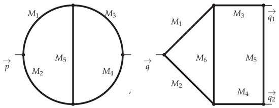
Figure 4. Two-loop two-point FI $I(M_1,M_2,M_3,M_4,M_5)$ and three-point FI $P(M_1,M_2,M_3,M_4,M_5,M_6)$ with $q_1^2=q_2^2=0$.

Below, we study the two-loop two-point and three-point FIs, which are special cases of the FIs shown in Figure 4. We call these:

$$\begin{array}{ccc}& & I_j=I(M_j=M\ne 0,M_p=0,p\ne j),I_{ij}=I(M_i=M_j=M\ne 0,M_p=0,p\ne i\ne j),\hfill \\ & & I_{ijs}=I(M_i=M_j=M_s=M\ne 0,M_p=0,p\ne i\ne j\ne s),\hfill \\ & & I_{ijst}=I(M_i=M_j=M_s=M_t=M\ne 0,M_p=0,p\ne i\ne j\ne s\ne t),\hfill \end{array}$$

(149)

$$\begin{array}{ccc}& & P_j=P(M_j=M\ne 0,M_p=0,p\ne j),P_{ij}=P(M_i=M_j=M\ne 0,M_p=0,p\ne i\ne j),\hfill \\ & & P_{ijs}=P(M_i=M_j=M_s=M\ne 0,M_p=0,p\ne i\ne j\ne s),\hfill \\ & & P_{ijst}=P(M_i=M_j=M_s=M_t=M\ne 0,M_p=0,p\ne i\ne j\ne s\ne t),\hfill \end{array}$$

(150)

Let us repeat here once again the importance of using the IBP procedure [19,87].

First of all, its use leads to relations between various FIs and, consequently, to the need to calculate only some of them, which in some sense are independent. These independent FIs (which, of course, can be chosen completely arbitrarily) are called master integrals [61].

Using the IBP relation [19,87] for the master integrals themselves leads to DEs for them with ITs containing simpler diagrams (see [23,24,25,26,27,28,29]). The term ‘simpler diagrams’ is applicable to diagrams that usually contain fewer propagators, and sometimes they can be represented as FIs with fewer loops and with some ’effective masses’ (see, for example, [62,107,108,109,110,123] and references therein). Using the IBP relation for IT diagrams leads to new DEs for them with new ITs containing even simpler FIs (≡simpler${}^2$ FIs). After repeating the procedure several times, in the last step, we obtain ITs containing mainly tadpoles, which can be easily calculated (see rule B in Section 6).

By solving the DEs in this last step, it is possible to reproduce FIs for the ITs of DEs in the previous step and so on. By repeating the procedure several times, one can obtain the results for the original FI.

8.1. Results Are in the Form of Series

Consider the integral $P_{x}126$ (massless and massive propagators are shown by thin and thick lines, respectively)

as a first example. It was calculated in Ref. [124] (see also [62,114]) and it has the series form (hereafter in Section 8 $x=q^2/m^2$):

$$\begin{array}{ccc}\hfill P_{125}& =& -\frac{N_d^2{\overline{\mu }}^{2\epsilon }}{{\left(q^2\right)}^{2+2\epsilon }}\sum _{n=1}\frac{{(-x)}^n}{2n}\frac{{(n!)}^2}{\left(2n\right)!}\{\frac{1}{{\epsilon }^2}-\frac{1}{\epsilon }(S_1+lnx)+4{\overline{S}}_1{S}_1-\frac{3}{2}\left(5S_1^2+S_2\right)-{\zeta }_2\hfill \\ & & +\frac{2}{n}{S}_1-S_{1}lnx+\frac{1}{2}{ln}^{2}x\}.\hfill \end{array}$$

(151)

where $S_i\left(n\right)$ is defined in Equation (35) and

$$S_i=S_i(n-1),{\overline{S}}_i=S_i(n-1)$$

(152)

and $\overline{\mu }=4\pi e^{-{\gamma }_E}\mu$ is the $\overline{MS}$-scale and ${\gamma }_E$ is the Euler constant.

8.2. Properties of Series

Series representations (as in Equation (151)) are convenient for calculating two-loop two-point FIs [23,24,25,26,27,28,29,123] and three-point FIs [62,107,108,124] with one non-zero mass. The calculation procedure using IBP relations and the construction of DEs based on it (see above) is very powerful, but rather complicated. However, there are some properties of series that either simplify calculations or sometimes allow a result to be obtained without direct calculations.

Indeed, the inverse mass decomposition of the two-loop two-point and three-point FIs with one non-zero mass can be represented as

$$\begin{array}{ccc}& & \mathrm{FI}=\frac{N_d^2{\overline{\mu }}^{2\epsilon }}{{\left(q^2\right)}^{2\alpha +2\epsilon }}\sum _{n=1}{C}_n{\left(\eta x\right)}^n\{F_0\left(n\right)+\left[lnx{F}_{1,1}\left(n\right)+\frac{1}{\epsilon }{F}_{1,2}\left(n\right)\right]\hfill \\ & & +\left[{ln}^{2}x{F}_{2,1}\left(n\right)+\frac{1}{\epsilon }lnx{F}_{2,2}\left(n\right)+\frac{1}{{\epsilon }^2}{F}_{2,3}\left(n\right)+\zeta \left(2\right)F_{2,4}\left(n\right)\right]+\dots \},\hfill \end{array}$$

(153)

where $\eta =1$ or $-1$ and $\alpha =1$ and 2 for two-point and three-point FIs, respectively.

We consider two-loop FIs without the cuts of three massive particles. Thus, the results of the considered FIs should be expressed as combinations of polylogarithms. Note that the three-point FIs are only considered with independent momenta $q_1$ and $q_2$ and the conditions $q_1^2=q_2^2=0$ and ${(q_1+q_2)}^2\equiv q^2\to 0$. Moreover,

$$\begin{array}{c}\hfill C_n=\frac{{(n!)}^2}{\left(2n\right)!}\equiv {\widehat{C}}_n\end{array}$$

(154)

for FIs having two-massive-particle-cuts ($2m$-cuts). For the FIs having only one-massive-particle-cuts (m-cuts), $C_n=1$.

For the m-cut case, the coefficients $F_{N,k}\left(n\right)$ should have the following form

$$\begin{array}{c}\hfill F_{N,k}\left(n\right)\sim \frac{S_{\pm a,\pm b,\pm c,\dots }}{n^d},\frac{\zeta (\pm a\pm b,\pm c,\dots )}{n^d},\end{array}$$

(155)

where $S_{\pm a,\pm b,\pm c,\dots }\equiv S_{\pm a,\pm b,\pm c,\dots }(j-1)$ are harmonic sums and $\zeta (\pm a,\pm b,\pm c,\dots )$ are the Euler–Zagier constants (also see Equation (35))

$$\begin{array}{ccc}& & S_{\pm a}\left(j\right)=\sum _{m=1}^j\frac{{(\pm 1)}^m}{m^a},S_{\pm a,\pm b,\pm c,\dots }\left(j\right)=\sum _{m=1}^j\frac{{(\pm 1)}^m}{m^a}{S}_{\pm b,\pm c,\dots }\left(m\right),\hfill \\ & & \zeta (\pm a)=\sum _{m=1}^{\infty }\frac{{(\pm 1)}^m}{m^a},\zeta (\pm a,\pm b,\pm c,\dots )=\sum _{m=1}^{\infty }\frac{{(\pm 1)}^m}{m^a}{S}_{\pm b,\pm c,\dots }(m-1).\hfill \end{array}$$

(156)

For the $2m$-cut case, the coefficients $F_{N,k}\left(n\right)$ are more complicated

$$\begin{array}{c}\hfill F_{N,k}\left(n\right)\sim \frac{S_{\pm a,\pm b,\pm c,\dots }}{n^d},\frac{V_{a,b,c,\dots }}{n^d},\frac{W_{a,b,c,\dots }}{n^d},\end{array}$$

(157)

where $W_{a,b,c,\dots }\equiv W_{a,b,c,\dots }(j-1)$ and $V_{a,b,c,\dots }\equiv V_{a,b,c,\dots }(j-1)$ with

$$\begin{array}{ccc}& & V_a\left(j\right)=\sum _{m=1}^j\frac{{\widehat{C}}_m}{m^a},V_{a,b,c,\dots }\left(j\right)=\sum _{m=1}^j\frac{{\widehat{C}}_m}{m^a}{S}_{b,c,\dots }\left(m\right),\hfill \end{array}$$

(158)

$$\begin{array}{ccc}& & W_a\left(j\right)=\sum _{m=1}^j\frac{{\widehat{C}}_m^{-1}}{m^a},W_{a,b,c,\dots }\left(j\right)=\sum _{m=1}^j\frac{{\widehat{C}}_m^{-1}}{m^a}{S}_{b,c,\dots }\left(m\right),\hfill \end{array}$$

(159)

The sums $\sim V_{a,b,c,\dots }$ and $\sim W_{a,b,c,\dots }$ can only appear in the $2m$-cut case. The source of their appearance is the product of two series with coefficients $C_n=1$ and $C_n={\widehat{C}}_n$, respectively

8.3. Additional Examples

Consider here the two-loop two-point FIs $I_1$ and $I_{12}$ calculated in [62] as additional examples

(160)

Their series expansions are

$$\begin{array}{ccc}\hfill I_1& =& -\frac{N_d^2{\overline{\mu }}^{2\epsilon }}{{\left(q^2\right)}^{1+2\epsilon }}\sum _{n=1}\frac{{(-x)}^n}{n}\left\{\frac{1}{2}{ln}^{2}x-\frac{2}{n}lnx+\zeta \left(2\right)+2S_2-2\frac{S_1}{n}+\frac{3}{n^2}\right\},\hfill \end{array}$$

(161)

$$\begin{array}{ccc}\hfill I_{12}& =& -\frac{N_d^2{\overline{\mu }}^{2\epsilon }}{{\left(q^2\right)}^{1+2\epsilon }}\sum _{n=1}\frac{{(-x)}^n}{n^2}\left\{\frac{1}{n}+\frac{{(n!)}^2}{\left(2n\right)!}\left(-2lnx-3W_1+\frac{2}{n}\right)\right\}.\hfill \end{array}$$

(162)

Equation (161) shows that, for the case where the functions $F_{N,k}\left(n\right)$ in Equation (153) have the form

$$\begin{array}{c}\hfill F_{N,k}\left(n\right)\sim \frac{1}{n^{3-N}},(N\ge 2),\end{array}$$

(163)

if we introduce the following complexity level of the used sums ($\overline{\mathsf{\Phi }}=(S,V,W)$)

$$\begin{array}{c}\hfill {\overline{\mathsf{\Phi }}}_{\pm a}\sim {\overline{\mathsf{\Phi }}}_{\pm a_1,\pm a_2}\sim {\overline{\mathsf{\Phi }}}_{\pm a_1,\pm a_2,\pm a_3,\dots ,\pm a_m}\sim {\zeta }_a\sim \frac{1}{n^a},(\sum _{i=1}^m{a}_i=a).\end{array}$$

(164)

The number $3-N$ determines the level of transcendentality (or complexity) or the weight of the coefficients $F_{N,k}\left(n\right)$ in Equation (153). This property significantly reduces the number of possible elements in $F_{N,k}\left(n\right)$. Moreover, the level of transcendentality decreases if we consider the FI singular parts and/or coefficients in the front of $\zeta$-functions or logarithm powers. Thus, having found the simplest parts, we can predict the rest using the results already obtained as ansatz, but using them with a higher level of transcendentality.

Other two-loop two-point FIs in [62] have similar representations. They were exactly calculated by the DE method [23,24,25,26,27,28,29].

Now, we consider two-loop three-point FIs, $P_5$ and $P_{12}$:

Their series expansions are (see [62]):

$$\begin{array}{ccc}\hfill P_5& =& \frac{N_d^2{\overline{\mu }}^{2\epsilon }}{{\left(q^2\right)}^{2+2\epsilon }}\sum _{n=1}\frac{x^n}{n}\{-6{\zeta }_3+2S_1{\zeta }_2+6S_3-2S_1{S}_2+4\frac{S_2}{n}-\frac{S_1^2}{n}+2\frac{S_1}{n^2}\hfill \\ & & +\left(-4S_2+S_1^2-2\frac{S_1}{n}\right)lnx+S_1{ln}^{2}x\},\hfill \\ \hfill P_{12}& =& \frac{N_d^2{\overline{\mu }}^{2\epsilon }}{{\left(q^2\right)}^{2+2\epsilon }}\sum _{n=1}\frac{{(-x)}^n}{n^2}\frac{{(n!)}^2}{\left(2n\right)!}\{\frac{2}{{\epsilon }^2}+\frac{2}{\epsilon }\left(S_1-3W_1+\frac{1}{n}-lnx\right)-6W_2-18W_{1,1}\hfill \\ & & -13S_2+S_1^2-6S_1{W}_1+2\frac{S_1}{n}+\frac{2}{n^2}-2\left(S_1+\frac{1}{n}\right)lnx+{ln}^{2}x\},\hfill \end{array}$$

(165)

In the last case, the coefficients $F_{N,k}\left(n\right)$ have the following form

$$\begin{array}{c}\hfill F_{N,k}\left(n\right)\sim \frac{1}{n^{4-N}},(N\ge 3),\end{array}$$

(166)

The FI $P_5$ (as well as FIs $P_1$, $P_3$, and $P_6$ in [62]) was calculated exactly by the DE method [23,24,25,26,27,28,29]. To calculate $P_{12}$ (as well as for all other FIs in [62]), we used the known results of several first terms in its inverse-mass expansion in Equation (153) and the following arguments:

• When a two-loop two-point FI with a ‘similar topology’ (for example, $I_{12}$ and $P_{12}$) has already been calculated, we consider a similar set of basic terms for the corresponding two-loop three-point FIs with a higher level of complexity.
• Let the considered FI contain the singularities and/or powers of logarithms.
  Since the coefficients in the front; the coefficients in the leading singularity; the coefficients in the front of the largest degree of the logarithm; or the coefficients in the largest $\zeta$-function are very simple, they can often be predicted directly from the first few coefficients of the considered expansion. Then, we can try to use them (with a corresponding increase in the level of complexity) to predict the rest of the diagram. If we need to find $\epsilon$-suppressed terms, we must further increase the level of transcendentality of the corresponding basic elements.

Furthermore, using the obtained results for $F_{N,k}\left(n\right)$ and several terms (usually less than 100) that were accurately calculated, we prepare a system of algebraic equations for the parameters of the ansatz. By solving the system, we can obtain analytic results for FIs without exact calculations. In this way, the results for many complicated two-loop three-point diagrams were obtained without direct calculations (see [62,107,108,124,125,126,127,128]).

We would like to note that similar properties have recently been observed [73,74,75,76] in the so-called double operator–product–expansion limit of some four-point diagrams.

In N = 4 SYM, the corresponding ansatz based on the properties of maximal transcendentality turns out to be stronger than in (155): the index b in (155) should be zero. This imposes very strong restrictions on the structure of the results [47,48,49,50,51], including the Yang–Baxter Q-function [129,130]. These constraints allow us to obtain the anomalous dimensions [49,50] in N = 4 SYM from the QCD results [52,53,54] up to three loops, as well as from the Bethe ansatz [131,132] up to seven loops [133,134,135,136,137]. In addition, there are other results (see Refs. [138,139,140,141,142,143,144,145]) related to the principle of maximum transcendentality [47,48,49,50,51].

8.4. Modern Method of Massive FIs

The coefficients of the inverse-mass expansions have the properties (163) and (166) in accordance with the rule (164). Note that this rule leads to a significant decrease in the possible coefficients. This limitation is due to the DE specific form for the FIs studied in this section. These DEs can be formally represented in the following form [55,56,57,58,59]

$$\begin{array}{c}\hfill \left((x+a)\frac{d}{dx}-\overline{k}\epsilon \right)\mathrm{FI}=\mathrm{simpler}\mathrm{FIs}(\equiv {\mathrm{FI}}_1),\end{array}$$

(167)

with some number a and some function $\overline{k}\left(x\right)$. We exactly show that the IT in the DE (167) contains only simpler diagrams. Note that the DE form is generated by the IBP relations for an internal n-leg single-loop subgraph, which in turn contains the product $k^{{\mu }_1}{k}^{{\mu }_2}{k}^{{\mu }_3}\dots k^{{\mu }_m}$ of the internal momentum k at $m=n-3$.

Indeed, for the usual values ${\alpha }_i=1+a_i\epsilon$ of the degrees of propagators of a subgraph with arbitrary $a_i$, the IBP relation (14) gives a coefficient $d-2{\alpha }_1-{\sum }_{i=2}^p{\alpha }_i+msin\epsilon$ for the FI itself with $m=n-3$. Important examples of applying this rule are FIs $I_1$, $I_{12}$ and $P_5$, $P_{12}$, $P_{126}$ (for the cases of $n=2$ and $n=3$), as well as FIs in [67] (for the cases $n=3$ and $n=4$). However, we note that the results for non-planar FIs (see Figure 3 in [62]) obey the property (166), but their subgraphs do not correspond to the obtained rule, which may be due to the on-shall vertex of the subgraph. However, this requires additional research.

Taking a set of simpler FIs, such as ${\mathrm{FI}}_1$ (collected in IT of the DE (167)), we obtain their structure like in Equation (166), but with a lower level of transcendentality.

So, the FIs ${\mathrm{FI}}_1$ must obey the following DE in the formal form

$$\begin{array}{c}\hfill \left((x+a_1)\frac{d}{dx}-{\overline{k}}_1\epsilon \right)\mathrm{F}{\mathrm{I}}_1={\mathrm{simpler}}^2\mathrm{FIs}(\equiv {\mathrm{FI}}_2).\end{array}$$

(168)

Thus, we have the DE set for all FIs ${\mathrm{FI}}_n$ as

$$\begin{array}{c}\hfill \left((x+a_n)\frac{d}{dx}-{\overline{k}}_n\epsilon \right)\mathrm{F}{\mathrm{I}}_n={\mathrm{simpler}}^{n+1}\mathrm{FIs}(\equiv {\mathrm{FI}}_{n+1}),\end{array}$$

(169)

with the last FI ${\mathrm{FI}}_{n+1}$ mainly containing tadpoles.

Following [146,147], we can replace the above system of inhomogeneous DEs as a homogeneous matrix DE (for complicated diagrams, see [148]; also see [149,150,151]. for methods to obtain homogeneous matrix DEs)

$$\begin{array}{c}\hfill \frac{d}{dx}\widehat{FI}-\epsilon \widehat{K}\widehat{FI}=0,\end{array}$$

(170)

for the vector

$$\begin{array}{c}\hfill \widehat{FI}=\left(\begin{array}{c}\mathrm{FI}\hfill \\ {\mathrm{FI}}_1/″\hfill \\ \dots \hfill \\ {\mathrm{FI}}_n/{″}^n\hfill \end{array}\right),\end{array}$$

where the matrix $\widehat{K}$ contains ${\overline{k}}_j/(x+a_j)$ as the it elements. The form was called the “canonic basic” (see (170)) and it is very popular now (see, for example, the review [152]).

In real calculations, we replace ${\mathrm{FI}}_n$ by

$${\mathrm{FI}}_n={\widetilde{\mathrm{FI}}}_n{\overline{\mathrm{FI}}}_n,$$

(171)

where the term ${\overline{\mathrm{FI}}}_n$ obeys the homogeneous Eq

$$\left((x+a_n)\frac{d}{dx}-{\overline{k}}_n\epsilon \right){\overline{\mathrm{FI}}}_n=0,$$

(172)

The replacement (171) simplifies the above DE (169) as

$$(x+a_n)\frac{d}{dx}{\widetilde{\mathrm{FI}}}_n={\widetilde{\mathrm{FI}}}_{n+1}\frac{{\overline{\mathrm{FI}}}_{n+1}}{{\overline{\mathrm{FI}}}_n},$$

(173)

having the it solution as

$${\widetilde{\mathrm{FI}}}_n\left(x\right)={\int }_0^x\frac{d{x}_1}{x_1+a_n}{\widetilde{\mathrm{FI}}}_{n+1}\left(x_1\right)\frac{{\overline{\mathrm{FI}}}_{n+1}\left(x_1\right)}{{\overline{\mathrm{FI}}}_n\left(x_1\right)}$$

(174)

There are often some abbreviations for ${\overline{\mathrm{FI}}}_{n+1}/{\overline{\mathrm{FI}}}_n$, so it is equal to 1. In this case, Equation (174) matches with the definition of Goncharov polylogarithms [153,154,155].

The results (161), (162), and (165) can be expressed in the form of Nilson [112] and Remiddi–Vermaseren [156] polylogarithms with the weigh $4-N$ (see [62,124]). A consideration of more complicated cases can be found in Ref. [157].

9. Conclusions

In this review, we reviewed effective methods for calculating FIs, as well as examples of the application of these methods. In the massless case, we studied the scalar two-point FIs with a TP in the numerator of one of the propagators, as well as FIs depending on the two momenta q and p when $p^2=0$. We also looked at FIs up to and including five loops that contribute to the $\beta$-function of the ${\phi }^4$ model. The FI results were analytically obtained in [8,13]; however, they were published without intermediate calculations. Our calculations are performed in detail.

In the case of massive propagators, we calculated of one of the complicated FIs that contribute to the ratio of the $\overline{MS}$ mass to the pole mass of the Higgs boson in the standard model in the limit of the heavy Higgs boson. The results for this FI were obtained by the DE method. They contain logarithms and dilogarithms with unusual arguments.

In addition, in the massive case, we studied the inverse-mass expansion for some two-loop two- and three-point FIs. For the massive FIs under consideration, we have introduced a definition of the level of transcendentality (or complexity), or weight, which is stored for any order of $\epsilon$. Moreover, it decreases in the front of logarithms or $\zeta$-values. We called this property transcendentality principle. Its usage leads to the possibility of obtaining results for most FIs without direct calculations.

The transcendentality principle is violated in physical models such as QCD, where the corresponding propagators (for both quarks and gluons) have momenta in their numerators, leading to the mixing of complexity levels. However, this property is restored after diagonalization for the corresponding anomalous dimensions and coefficient functions in $N=4$ SYM, which is an excellent, but so far little-studied property.

References

- Peterman, A. Renormalization Group and the Deep Structure of the Proton. Phys. Rep. 1979, 53, 157–248. [Google Scholar] [CrossRef]
- ’t Hooft, G.; Veltman, M.J.G. Regularization and Renormalization of Gauge Fields. Nucl. Phys. B 1972, 44, 189–213. [Google Scholar] [CrossRef]
- Bollini, C.G.; Giambiagi, J.J. Dimensional Renormalization: The Number of Dimensions as a Regularizing Parameter. Nuovo Cim. B 1972, 12, 20–26. [Google Scholar] [CrossRef]
- Cicuta, G.M.; Montaldi, E. Analytic renormalization via continuous space dimension. Lett. Nuovo Cim. 1972, 4, 329–332. [Google Scholar] [CrossRef]
- Hooft, G. Dimensional regularization and the renormalization group. Nucl. Phys. B 1973, 61, 455–468. [Google Scholar] [CrossRef]
- D’Eramo, M.; Peliti, L. Theoretical Predictions for Critical Exponents at the Lambda Point of Bose Liquids. Lett. Nuovo Cim. 1971, 2, 878–880. [Google Scholar] [CrossRef]
- Vasiliev, A.N.; Khonkonen, Y.R. 1/N Expansion: Calculation of the Exponents Eta Furthermore, Nu in the Order 1/N**2 for Arbitrary Number of Dimensions. Theor. Math. Phys. 1981, 47, 465–475. [Google Scholar] [CrossRef]
- Kazakov, D.I. The Method of Uniqueness, a New Powerful Technique for Multiloop Calculations. Phys. Lett. B 1983, 133, 406–410. [Google Scholar] [CrossRef]
- Kazakov, D.I. Calculation of Feynman Integrals by the Method of ‘uniqueness’. Theor. Math. Phys. 1984, 58, 223–230, [Teor. Mat. Fiz. 1984, 58, 343]. [Google Scholar] [CrossRef]
- Usyukina, N.I. Calculation of Many Loop Diagrams of Perturbation Theory. Theor. Math. Phys. 1983, 54, 78–81, [Teor. Mat. Fiz. 1983, 54, 124]. [Google Scholar] [CrossRef]
- Belokurov, V.V.; Usyukina, N.I.J. Calculation of Ladder Diagrams in Arbitrary Order. J. Phys. A 1983, 16, 2811. [Google Scholar] [CrossRef]
- Belokurov, V.V.; Usyukina, N.I. An Algorithm for Calculating Massless Feynman Diagrams. Theor. Math. Phys. 1989, 79, 385–391, [Teor. Mat. Fiz. 1989, 79, 63]. [Google Scholar]
- Kazakov, D.I. Multiloop Calculations: Method of Uniqueness and Functional Equations. Theor. Math. Phys. 1985, 62, 84–89, [Teor. Mat. Fiz. 1984, 62, 127]. [Google Scholar] [CrossRef]
- Kotikov, A.V. The Gegenbauer polynomial technique: The Evaluation of a class of Feynman diagrams. Phys. Lett. B 1996, 375, 240–248. [Google Scholar] [CrossRef][Green Version]
- Kotikov, A.V.; Teber, S. New Results for a Two-Loop Massless Propagator-Type Feynman Diagram. Theor. Math. Phys. 2018, 194, 284–294, [Teor. Mat. Fiz. 2018, 194, 331]. [Google Scholar] [CrossRef]
- Kotikov, A.V.; Teber, S. Multi-loop techniques for massless Feynman diagram calculations. Phys. Part. Nucl. 2019, 50, 1–41. [Google Scholar] [CrossRef]
- Kotikov, A.V. Differential Equations and Feynman Integrals. arXiv 2012, arXiv:2102.07424. [Google Scholar]
- Ryder, L.H. Quantum Field Theory; Cambridge University Press: Cambridge, UK, 1996. [Google Scholar]
- Chetyrkin, K.G.; Tkachov, F.V. Integration By Parts: The Algorithm to Calculate Beta Functions in 4 Loops. Nucl. Phys. B 1981, 192, 159–204. [Google Scholar] [CrossRef]
- Kazakov, D.I.; Kotikov, A.V. The Method of Uniqueness: Multiloop Calculations in QCD. Theor. Math. Phys. 1988, 73, 1264–1274. [Google Scholar] [CrossRef]
- Kazakov, D.I.; Kotikov, A.B. Total αs Correction to Deep Inelastic Scattering Cross-section Ratio R = σL/σT in QCD. Nucl. Phys. B 1988, 307, 721–762, Erratum in Nucl. Phys. B 1990, 345, 299. [Google Scholar] [CrossRef]
- Kotikov, A.V. The Calculation of Moments of Structure Function of Deep Inelastic Scattering in QCD. Theor. Math. Phys. 1989, 78, 134–143. [Google Scholar] [CrossRef]
- Kotikov, A.V. Differential equations method: New technique for massive Feynman diagrams calculation. Phys. Lett. B 1991, 254, 158–164. [Google Scholar] [CrossRef]
- Kotikov, A.V. Differential equations method: The Calculation of vertex type Feynman diagrams. Phys. Lett. B 1991, 259, 314–322. [Google Scholar] [CrossRef]
- Kotikov, A.V. Differential equation method: The Calculation of N point Feynman diagrams. Phys. Lett. B 1991, 267, 123–127. [Google Scholar] [CrossRef]
- Kotikov, A.V. New method of massive N point Feynman diagrams calculation. Mod. Phys. Lett. A 1991, 6, 3133–3141. [Google Scholar] [CrossRef]
- Remiddi, E. Differential equations for Feynman graph amplitudes. Nuovo Cim. A 1997, 110, 1435–1452. [Google Scholar] [CrossRef]
- Kotikov, A.V. New method of massive Feynman diagrams calculation. Mod. Phys. Lett. A 1991, 6, 677–692. [Google Scholar] [CrossRef]
- Kotikov, A.V. New method of massive Feynman diagrams calculation. Vertex type functions. Int. J. Mod. Phys. A 1992, 7, 1977–1991. [Google Scholar] [CrossRef]
- Gorishnii, S.G.; Larin, S.A.; Tkachov, F.V.; Chetyrkin, K.G. Five Loop Renormalization Group Calculations in the gϕ4 in Four-dimensions Theory. Phys. Lett. B 1983, 132, 351–354. [Google Scholar]
- Tarasov, O.V. Connection between Feynman integrals having different values of the space-time dimension. Phys. Rev. D 1996, 54, 6479. [Google Scholar] [CrossRef]
- Tarasov, O.V. Generalized recurrence relations for two loop propagator integrals with arbitrary masses. Nucl. Phys. B 1997, 502, 455–482. [Google Scholar] [CrossRef]
- Lee, R.N. Presenting LiteRed: A tool for the Loop InTEgrals REDuction. arXiv 2012, arXiv:1212.2685. [Google Scholar]
- Lee, R.N. LiteRed 1.4: A powerful tool for reduction of multiloop integrals. J. Phys. Conf. Ser. 2014, 523, 012059. [Google Scholar] [CrossRef]
- Lee, R.N.; Smirnov, A.V.; Smirnov, V.A. Analytic Results for Massless Three-Loop Form Factors. J. High Energy Phys. JHEP 2010, 2010, 020. [Google Scholar] [CrossRef]
- Kotikov, A.V.; Lipatov, L.N. NLO corrections to the BFKL equation in QCD and in supersymmetric gauge theories. Nucl. Phys. B 2000, 582, 19–43. [Google Scholar] [CrossRef]
- Lipatov, L.N. Reggeization of the Vector Meson and the Vacuum Singularity in Nonabelian Gauge Theories. Sov. J. Nucl. Phys. 1976, 23, 338–345. [Google Scholar]
- Fadin, V.S.; Kuraev, E.A.; Lipatov, L.N. On the Pomeranchuk Singularity in Asymptotically Free Theories. Phys. Lett. B 1975, 60, 50–52. [Google Scholar] [CrossRef]
- Kuraev, E.A.; Lipatov, L.N.; Fadin, V.S. Multi-Reggeon Processes in the Yang-Mills Theory. Sov. Phys. JETP 1976, 44, 443–450. [Google Scholar]
- Kuraev, E.A.; Lipatov, L.N.; Fadin, V.S. The Pomeranchuk Singularity in Nonabelian Gauge Theories. Sov. Phys. JETP 1977, 45, 199–204. [Google Scholar]
- Balitsky, I.I.; Lipatov, L.N. The Pomeranchuk Singularity in Quantum Chromodynamics. Sov. J. Nucl. Phys. 1978, 28, 822–829. [Google Scholar]
- Balitsky, I.I.; Lipatov, L.N. Calculation of meson meson interaction cross-section in quantum chromodynamics. JETP Lett. 1979, 30, 355. [Google Scholar]
- Fadin, V.S.; Lipatov, L.N. BFKL pomeron in the next-to-leading approximation. Phys. Lett. B 1998, 429, 127–134. [Google Scholar] [CrossRef]
- Camici, G.; Ciafaloni, M. Energy scale(s) and next-to-leading BFKL equation. Phys. Lett. B 1998, 430, 349–354. [Google Scholar]
- Brink, L.; Schwarz, J.H.; Scherk, J. Supersymmetric Yang-Mills Theories. Nucl. Phys. B 1977, 121, 77–92. [Google Scholar] [CrossRef]
- Gliozzi, F.; Scherk, J.; Olive, D.I. Supersymmetry, Supergravity Theories and the Dual Spinor Model. Nucl. Phys. B 1977, 122, 253–290. [Google Scholar] [CrossRef]
- Kotikov, A.V.; Lipatov, L.N. DGLAP and BFKL equations in the N = 4 supersymmetric gauge theory. Nucl. Phys. B 2003, 661, 19–61. [Google Scholar] [CrossRef]
- Kotikov, A.V.; Lipatov, L.N. DGLAP and BFKL evolution equations in the N = 4 supersymmetric gauge theory. arXiv 2001, arXiv:hep-ph/0112346. [Google Scholar]
- Kotikov, A.V.; Lipatov, L.N.; Velizhanin, V.N. Anomalous dimensions of Wilson operators in N = 4 SYM theory. Phys. Lett. B 2003, 557, 114–120. [Google Scholar] [CrossRef]
- Kotikov, A.V.; Lipatov, L.N.; Onishchenko, A.I.; Velizhanin, V.N. Three loop universal anomalous dimension of the Wilson operators in N = 4 SUSY Yang-Mills model. Phys. Lett. B 2004, 595, 521–529. [Google Scholar] [CrossRef]
- Bianchi, L.; Forini, V.; Kotikov, A.V. On DIS Wilson coefficients in N = 4 super Yang–Mills theory. Phys. Lett. B 2013, 725, 394–401. [Google Scholar] [CrossRef]
- Moch, S.; Vermaseren, J.A.M.; Vogt, A. The Three loop splitting functions in QCD: The Nonsinglet case. Nucl. Phys. B 2004, 688, 101–134. [Google Scholar] [CrossRef]
- Vogt, A.; Moch, S.; Vermaseren, J.A.M. The Three-loop splitting functions in QCD: The Singlet case. Nucl. Phys. B 2004, 691, 129–181. [Google Scholar] [CrossRef]
- Vermaseren, J.A.M.; Vogt, A.; Moch, S. The Third-order QCD corrections to deep-inelastic scattering by photon exchange. Nucl. Phys. B 2005, 724, 3–182. [Google Scholar] [CrossRef]
- Kotikov, A.V. The Property of maximal transcendentality in the N = 4 Supersymmetric Yang–Mills. In Subtleties in Quantum Field Theory; Diakonov, D., Ed.; PNPI: Gatchina, Russia, 2010; pp. 150–174. [Google Scholar]
- Kotikov, A.V. The property of maximal transcendentality: Calculation of anomalous dimensions in the = 4 SYM and master integrals. Phys. Part. Nucl. 2013, 44, 374–385. [Google Scholar] [CrossRef]
- Kotikov, A.V.; Onishchenko, A.I. DGLAP and BFKL equations in = 4 SYM: From weak to strong coupling. arXiv 2019, arXiv:1908.05113. [Google Scholar]
- Kotikov, A.V. The property of maximal transcendentality: Calculation of master integrals. Theor. Math. Phys. 2013, 176, 913–921. [Google Scholar] [CrossRef]
- Kotikov, A.V. The property of maximal transcendentality: Calculation of Feynman integrals. Theor. Math. Phys. 2017, 190, 391–401. [Google Scholar] [CrossRef]
- Kotikov, A.V. Some Examples of Calculation of Massless and Massive Feynman Integrals. Particles 2021, 4, 361–380. [Google Scholar] [CrossRef]
- Broadhurst, D.J. The Master Two Loop Diagram with Masses. Z. Phys. C 1990, 47, 115–124. [Google Scholar] [CrossRef]
- Fleischer, J.; Kotikov, A.V.; Veretin, O.L. Analytic two loop results for selfenergy type and vertex type diagrams with one nonzero mass. Nucl. Phys. B 1999, 547, 343–374. [Google Scholar] [CrossRef]
- Kotikov, A.V. About calculation of massless and massive Feynman integrals. Particles 2020, 3, 394–443. [Google Scholar] [CrossRef]
- Eden, B.; Heslop, P.; Korchemsky, G.P.; Sokatchev, E. Hidden symmetry of four-point correlation functions and amplitudes in N = 4 SYM. Nucl. Phys. B 2012, 862, 193–231. [Google Scholar] [CrossRef]
- Dixon, L.J. Scattering amplitudes: The most perfect microscopic structures in the universe. J. Phys. A 2011, 44, 454001. [Google Scholar] [CrossRef]
- Dixon, L.J.; Drummond, J.M.; Henn, J.M. Analytic result for the two-loop six-point NMHV amplitude in N = 4 super Yang–Mills theory. J. High Energy Phys. JHEP 2012, 2012, 024. [Google Scholar] [CrossRef]
- Gehrmann, T.; Henn, J.M.; Huber, T. The three-loop form factor in N = 4 super Yang–Mills. J. High Energy Phys. JHEP 2012, 2012, 101. [Google Scholar] [CrossRef]
- Brandhuber, A.; Travaglini, G.; Yang, G. Analytic two-loop form factors in N = 4 SYM. J. High Energy Phys. JHEP 2012, 2012, 082. [Google Scholar] [CrossRef]
- Henn, J.M.; Moch, S.; Naculich, S.G. Form factors and scattering amplitudes in N = 4 SYM in dimensional and massive regularizations. J. High Energy Phys. JHEP 2011, 2011, 024. [Google Scholar] [CrossRef]
- Schlotterer, O.; Stieberger, S.J. Motivic Multiple Zeta Values and Superstring Amplitudes. J. Phys. A 2013, 46, 475401. [Google Scholar] [CrossRef]
- Broedel, J.; Schlotterer, O.; Stieberger, S. Polylogarithms, Multiple Zeta Values and Superstring Amplitudes. Fortsch. Phys. 2013, 61, 812–870. [Google Scholar] [CrossRef]
- Stieberger, S.; Taylor, T.R. Maximally Helicity Violating Disk Amplitudes, Twistors and Transcendental Integrals. Phys. Lett. B 2012, 716, 236–239. [Google Scholar] [CrossRef]
- Eden, B. Three-loop universal structure constants in N = 4 susy Yang–Mills theory. arXiv 2012, arXiv:1207.3112. [Google Scholar]
- Ambrosio, R.G.; Eden, B.; Goddard, T.; Heslop, P.; Taylor, C. Local integrands for the five-point amplitude in planar N = 4 SYM up to five loops. J. High Energy Phys. JHEP 2015, 2015, 116. [Google Scholar] [CrossRef]
- Chicherin, D.; Doobary, R.; Eden, B.; Heslop, P.; Korchemsky, G.P.; Sokatchev, E. Bootstrapping correlation functions in N = 4 SYM. J. High Energy Phys. JHEP 2016, 2016, 031. [Google Scholar] [CrossRef]
- Eden, B.; Sfondrini, A. Three-point functions in = 4 SYM: The hexagon proposal at three loops. J. High Energy Phys. JHEP 2016, 2016, 165. [Google Scholar] [CrossRef]
- Chetyrkin, K.G.; Kataev, A.L.; Tkachov, F.V. New Approach to Evaluation of Multiloop Feynman Integrals: The Gegenbauer Polynomial x Space Technique. Nucl. Phys. B 1980, 174, 345–377. [Google Scholar] [CrossRef]
- Kotikov, A.V. Critical behavior of 3-D electrodynamics. JETP Lett. 1993, 58, 731, [Pisma Zh. Eksp. Teor. Fiz. 1993, 58, 785]. [Google Scholar]
- Kotikov, A.V. On the Critical Behavior of (2+1)-Dimensional QED. Phys. Atom. Nucl. 2012, 75, 890–892. [Google Scholar] [CrossRef]
- Kotikov, A.V.; Shilin, V.I.; Teber, S. Critical behavior of (2+1)-dimensional QED: 1/Nf corrections in the Landau gauge. Phys. Rev. D 2016, 94, 056009, Erratum in Phys. Rev. D 2019, 99, 119901. [Google Scholar] [CrossRef]
- Kotikov, A.V.; Teber, S. Critical behavior of (2+1)-dimensional QED: 1/Nf corrections in an arbitrary nonlocal gauge. Phys. Rev. D 2016, 94, 114011, Addendum in Phys. Rev. D 2019, 99, 059902. [Google Scholar] [CrossRef]
- Kotikov, A.V.; Teber, S. Two-loop fermion self-energy in reduced quantum electrodynamics and application to the ultrarelativistic limit of graphene. Phys. Rev. D 2014, 89, 065038. [Google Scholar] [CrossRef]
- Derkachev, S.E.; Ivanov, A.V.; Shumilov, L.A. Mellin–Barnes transformation for two-loop master-diagrams. Zap. Nauchn. Semin. 2020, 494, 144–167. [Google Scholar] [CrossRef]
- Derkachev, S.E.; Ivanov, A.V.; Shumilov, L.A. Mellin–Barnes Transformation for Two-Loop Master-Diagram. J. Math. Sci. 2022, 264, 298–312. [Google Scholar] [CrossRef]
- Derkachov, S.E.; Isaev, A.P.; Shumilov, L.A. Ladder and zig-zag Feynman diagrams, operator formalism and conformal triangles. J. High Energy Phys. JHEP 2023, 2023, 059. [Google Scholar] [CrossRef]
- Teber, S.; Kotikov, A.V. The method of uniqueness and the optical conductivity of graphene: New application of a powerful technique for multiloop calculations. Theor. Math. Phys. 2017, 190, 446–457. [Google Scholar] [CrossRef]
- Tkachov, F.V. A Theorem on Analytical Calculability of Four Loop Renormalization Group Functions. Phys. Lett. B 1981, 100, 65–68. [Google Scholar] [CrossRef]
- Broadhurst, D.J. Exploiting the 1.440 Fold Symmetry of the Master Two Loop Diagram. Z. Phys. C 1986, 32, 249–253. [Google Scholar] [CrossRef]
- Gorishnii, S.G.; Isaev, A.P. On an Approach to the Calculation of Multiloop Massless Feynman Integrals. Theor. Math. Phys. 1985, 62, 232–240, [Teor. Mat. Fiz. 1985, 62, 345]. [Google Scholar] [CrossRef]
- Kazakov, D.I. Analytical Methods for Multiloop Calculations: Two Lectures on The Method of Uniqueness. JINR-E2-84-410. 1984. Available online: https://inspirehep.net/literature/203305 (accessed on 25 May 2023).
- Broadhurst, D.J. Dimensionally continued multiloop gauge theory. arXiv 1999, arXiv:hep-th/9909185. [Google Scholar]
- Kotikov, A.V.; Teber, S. Landau-Khalatnikov-Fradkin transformation and the mystery of even ζ-values in Euclidean massless correlators. Phys. Rev. D 2019, 100, 105017. [Google Scholar] [CrossRef]
- Kazakov, D.I.; Kotikov, A.V. On the value of the alpha-s correction to the Callan-Gross relation. Phys. Lett. B 1992, 291, 171–176. [Google Scholar] [CrossRef]
- Gorishnii, S.G.; Larin, S.A.; Tkachov, F.V. The Algorithm for Ope Coefficient Functions in the Ms Scheme. Phys. Lett. B 1983, 124, 217–220. [Google Scholar] [CrossRef]
- Gorishnii, S.G.; Larin, S.A. Coefficient Functions of Asymptotic Operator Expansions in Minimal Subtraction Scheme. Nucl. Phys. B 1987, 283, 452–476. [Google Scholar] [CrossRef]
- Tkachov, F.V. On The Operator Product Expansion in the Ms Scheme. Phys. Lett. B 1983, 124, 212–216. [Google Scholar] [CrossRef]
- Chetyrkin, K.G. Infrared R*—operation and operator product expansion in the minimal subtraction scheme. Phys. Lett. B 1983, 126, 371–375. [Google Scholar] [CrossRef]
- Bogoliubov, N.N.; Parasiuk, O.S. On the Multiplication of the causal function in thequantum theory of fields. Acta Math. 1957, 97, 227–266. [Google Scholar]
- Hepp, K. Proof of the Bogolyubov-Parasiuk theorem on renormalization. Commun. Math. Phys. 1966, 2, 301–326. [Google Scholar] [CrossRef]
- Zimmermann, W. Convergence of Bogoliubov’s method of renormalization in momentumspace. Commun. Math. Phys. 1969, 15, 208–234. [Google Scholar] [CrossRef]
- Vladimirov, A.A. Method for Computing Renormalization Group Functions in Dimen-sional Renormalization Scheme. Theor. Math. Phys. 1980, 43, 417–422. [Google Scholar] [CrossRef]
- Chetyrkin, K.G.; Tkachov, F.V. Infrared R Operation Furthermore, Ultraviolet CountertermsIn The Ms Scheme. Phys. Lett. B 1982, 114, 340–344. [Google Scholar] [CrossRef]
- Chetyrkin, K.G.; Smirnov, V.A. R* Operation Corrected. Phys. Lett. B 1984, 144, 419–424. [Google Scholar] [CrossRef]
- Smirnov, V.A.; Chetyrkin, K.G. R* Operation in the Minimal Subtraction Scheme. Theor. Math. Phys. 1985, 63, 462–469. [Google Scholar] [CrossRef]
- Chetyrkin, K.G. Combinatorics of R-, R−1-, and R*-operations and asymptotic expan-sions of feynman integrals in the limit of large momenta and masses. arXiv 2017, arXiv:1701.08627. [Google Scholar]
- Henn, J.M.; Plefka, J.C. Scattering Amplitudes in Gauge Theories; Lecture Notes in Physics; Springer: Berlin, Germany, 2014; Volume 883. [Google Scholar]
- Kniehl, B.A.; Kotikov, A.V.; Onishchenko, A.; Veretin, O. Two-loop sunset diagrams with three massive lines. Nucl. Phys. B 2006, 738, 306–316. [Google Scholar] [CrossRef]
- Kniehl, B.A.; Kotikov, A.V.; Onishchenko, A.I.; Veretin, O.L. Two-loop diagrams in non-relativistic QCD with elliptics. Nucl. Phys. B 2019, 948, 114780. [Google Scholar] [CrossRef]
- Kniehl, B.A.; Kotikov, A.V. Calculating four-loop tadpoles with one non-zero mass. Phys. Lett. B 2006, 638, 531–537. [Google Scholar] [CrossRef]
- Kniehl, B.A.; Kotikov, A.V. Counting master integrals: Integration-by-parts procedure with effective mass. Phys. Lett. B 2012, 712, 233–234. [Google Scholar] [CrossRef]
- Lewin, L. Polylogarithms and Associated Functions; North Holland: Amsterdam, The Netherlands, 1981. [Google Scholar]
- Devoto, A.; Duke, D.W. Table of Integrals and Formulae for Feynman Diagram Calculations. Riv. Nuovo Cim. 1984, 7, 1–39. [Google Scholar] [CrossRef]
- Campert, L.G.J.; Moriello, F.; Kotikov, A. Sunrise integrals with two internal masses and pseudo-threshold kinematics in terms of elliptic polylogarithms. J. High Energy Phys. JHEP 2021, 2021, 072. [Google Scholar] [CrossRef]
- Kotikov, A.; Kuhn, J.H.; Veretin, O. Two-Loop Formfactors in Theories with Mass Gap and Z-Boson Production. Nucl. Phys. B 2008, 788, 47–62. [Google Scholar] [CrossRef][Green Version]
- Aglietti, U.; Bonciani, R. Master integrals with one massive propagator for the two loop electroweak form-factor. Nucl. Phys. B 2003, 668, 3–76. [Google Scholar] [CrossRef]
- Aglietti, U.; Bonciani, R.; Degrassi, G.; Vicini, A. Two loop light fermion contribution to Higgs production and decays. Phys. Lett. B 2004, 595, 432–441. [Google Scholar] [CrossRef]
- Aglietti, U.; Bonciani, R.; Degrassi, G.; Vicini, A. Master integrals for the two-loop light fermion contributions to gg —> H and H —> gamma gamma. Phys. Lett. B 2004, 600, 57–64. [Google Scholar] [CrossRef]
- Aglietti, U.; Bonciani, R.; Degrassi, G.; Vicini, A. Analytic Results for Virtual QCD Corrections to Higgs Production and Decay. J. High Energy Phys. JHEP 2007, 2007, 021. [Google Scholar] [CrossRef]
- Lee, R.N.; Schwartz, M.D.; Zhang, X. Compton Scattering Total Cross Section at Next-to-Leading Order. Phys. Rev. Lett. 2021, 126, 211801. [Google Scholar] [CrossRef]
- Blumlein, J.; Schneider, C. Analytic Computing Methods for Precision Calculations in Quantum Field Theory. Int. J. Mod. Phys. 2018, A33, 1830015. [Google Scholar] [CrossRef]
- Ablinger, J.; Blümlein, J.; Schneider, C. Iterated integrals over letters induced by quadratic forms. Phys. Rev. D 2021, 103, 096025. [Google Scholar] [CrossRef]
- Ablinger, J.; Blumlein, J.; Schneider, C.J. Harmonic Sums and Polylogarithms Generated by Cyclotomic Polynomials. Math. Phys. 2011, 52, 102301. [Google Scholar] [CrossRef]
- Fleischer, J.; Kalmykov, M.Y.; Kotikov, A.V. Two-loop self-energy master integrals on shell. Phys. Lett. B 1999, 462, 169–177. [Google Scholar] [CrossRef][Green Version]
- Fleischer, J.; Kotikov, A.V.; Veretin, O.L. The differential equation method: Calculation of vertex-type diagrams with one non-zero mass. Phys. Lett. B 1998, 417, 163–172. [Google Scholar] [CrossRef]
- Kniehl, B.A.; Kotikov, A.V.; Onishchenko, A.I.; Veretin, O.L. Strong-coupling constant with flavor thresholds at five loops in the MS-bar scheme. Phys. Rev. Lett. 2006, 97, 042001. [Google Scholar] [CrossRef]
- Kniehl, B.A.; Kotikov, A.V.; Merebashvili, Z.V.; Veretin, O.L. Heavy-quark pair production in polarized photon-photon collisions at next-to-leading order: Fully integrated total cross sections. Phys. Rev. D 2009, 79, 114032. [Google Scholar] [CrossRef]
- Kniehl, B.A.; Kotikov, A.V.; Veretin, O.L. Orthopositronium lifetime: Analytic results in O(α) and O(α3ln(α)). Phys. Rev. Lett. 2008, 101, 193401. [Google Scholar] [CrossRef]
- Kniehl, B.A.; Kotikov, A.V.; Veretin, O.L. Orthopositronium lifetime at O(alpha) and O(alpha3 ln(alpha)) in closed form. Phys. Rev. A 2009, 80, 052501. [Google Scholar] [CrossRef]
- Kotikov, A.V.; Rej, A.; Zieme, S. Analytic three-loop Solutions for N = 4 SYM Twist Operators. Nucl. Phys. B 2009, 813, 460–483. [Google Scholar] [CrossRef]
- Beccaria, M.; Belitsky, A.V.; Kotikov, A.V.; Zieme, S. Analytic solution of the multiloop Baxter equation. Nucl. Phys. B 2010, 827, 565–606. [Google Scholar] [CrossRef][Green Version]
- Staudacher, M. The Factorized S-matrix of CFT/AdS. J. High Energy Phys. JHEP 2005, 2005, 054. [Google Scholar] [CrossRef]
- Beisert, N.; Staudacher, M. Long-range psu(2,2|4) Bethe Ansatze for gauge theory and strings. Nucl. Phys. B 2005, 727, 1–62. [Google Scholar] [CrossRef]
- Kotikov, A.V.; Lipatov, L.N.; Rej, A.; Staudacher, M.; Velizhanin, V.N. Dressing and wrapping. J. Stat. Mech. 2007, 0710, P10003. [Google Scholar] [CrossRef]
- Bajnok, Z.; Janik, R.A.; Lukowski, T. our-loop perturbative Konishi from strings and finite size effects for multiparticle states. Nucl. Phys. B 2009, 816, 376–398. [Google Scholar] [CrossRef][Green Version]
- Lukowski, T.; Rej, A.; Velizhanin, V.N. Five-Loop Anomalous Dimension of Twist-Two Operators. Nucl. Phys. B 2010, 831, 105–132. [Google Scholar] [CrossRef][Green Version]
- Marboe, C.; Velizhanin, V.; Volin, D. Six-loop anomalous dimension of twist-two operators in planar = 4 SYM theory. J. High Energy Phys. JHEP 2015, 2015, 084. [Google Scholar] [CrossRef]
- Marboe, C.; Velizhanin, V. Twist-2 at seven loops in planar = 4 SYM theory: Full result and analytic properties. J. High Energy Phys. JHEP 2016, 2016, 013. [Google Scholar] [CrossRef]
- Kotikov, A.V.; Lipatov, L.N. On the highest transcendentality in N = 4 SUSY. Nucl. Phys. B 2007, 769, 217–255. [Google Scholar] [CrossRef]
- Benna, M.K.; Benvenuti, S.; Klebanov, I.R.; Scardicchio, A. A Test of the AdS/CFT correspondence using high-spin operators. Phys. Rev. Lett. 2007, 98, 131603. [Google Scholar] [CrossRef]
- Basso, B.; Korchemsky, G.P.; Kotanski, J. Cusp anomalous dimension in maximally supersymmetric Yang–Mills theory at strong coupling. Phys. Rev. Lett. 2008, 100, 091601. [Google Scholar] [CrossRef]
- Basso, B.; Korchemsky, G.P. Embedding nonlinear O(6) sigma model into N = 4 super-Yang–Mills theory. Nucl. Phys. B 2009, 807, 397–423. [Google Scholar] [CrossRef]
- Costa, M.S.; Goncalves, V.; Penedones, J. Conformal Regge theory. J. High Energy Phys. JHEP 2012, 2012, 091. [Google Scholar] [CrossRef]
- Kotikov, A.V.; Lipatov, L.N. Pomeron in the N = 4 supersymmetric gauge model at strong couplings. Nucl. Phys. B 2013, 874, 889–904. [Google Scholar] [CrossRef]
- Gromov, N.; Levkovich-Maslyuk, F.; Sizov, G.; Valatka, S. Quantum spectral curve at work: From small spin to strong coupling in = 4 SYM. J. High Energy Phys. JHEP 2014, 2014, 156. [Google Scholar] [CrossRef]
- Alday, L.F.; Hansen, T. The AdS Virasoro-Shapiro Amplitude. arXiv 2023, arXiv:2306.12786. [Google Scholar] [CrossRef]
- Henn, J.M. Multiloop integrals in dimensional regularization made simple. Phys. Rev. Lett. 2013, 110, 251601. [Google Scholar] [CrossRef]
- Henn, J.M. Lectures on differential equations for Feynman integrals. J. Phys. A 2015, 48, 153001. [Google Scholar] [CrossRef]
- Adams, L.; Weinzierl, S. The ε-form of the differential equations for Feynman integrals in the elliptic case. Phys. Lett. B 2018, 781, 270–278. [Google Scholar] [CrossRef]
- Lee, R.N. Reducing differential equations for multiloop master integrals. J. High Energy Phys. JHEP 2015, 2015, 108. [Google Scholar] [CrossRef]
- Lee, R.N. Symmetric ϵ- and (ϵ+1/2)-forms and quadratic constraints in “elliptic” sectors. J. High Energy Phys. JHEP 2018, 2018, 176. [Google Scholar] [CrossRef]
- Lee, R.N.; Onishchenko, A.I. ϵ-regular basis for non-polylogarithmic multiloop integrals and total cross section of the process e+e−→2(QQ). J. High Energy Phys. JHEP 2019, 2019, 084. [Google Scholar] [CrossRef]
- Badger, S.; Henn, J.; Plefka, J.; Zoia, S. Scattering Amplitudes in Quantum Field Theory. arXiv 2023, arXiv:2306.05976. [Google Scholar]
- Duhr, C. Mathematical aspects of scattering amplitudes. arXiv 2014, arXiv:1411.7538. [Google Scholar]
- Goncharov, A.B. Multiple polylogarithms and mixed Tate motives. arXiv 2001, arXiv:math/0103059. [Google Scholar]
- Goncharov, A.B. Multiple polylogarithms, cyclotomy and modular complexes. Math. Res. Lett. 1998, 5, 497–516. [Google Scholar] [CrossRef]
- Remiddi, E.; Vermaseren, J.A.M. Harmonic polylogarithms. Int. J. Mod. Phys. A 2000, 15, 725–754. [Google Scholar] [CrossRef]
- Davydychev, A.I.; Kalmykov, M.Y. Massive Feynman diagrams and inverse binomial sums. Nucl. Phys. B 2004, 699, 3–64. [Google Scholar] [CrossRef]
- Kotikov, A.V. Gluon distribution for small x. Phys. At. Nucl. 1994, 57, 133. [Google Scholar]
- Kotikov, A.V.; Velizhanin, V.N. Analytic continuation of the Mellin moments of deep inelastic structure functions. arXiv 2005, arXiv:hep-ph/0501274. [Google Scholar]
- Parisi, G.; Sourlas, N. A Simple Parametrization of the Q2 Dependence of the Quark Distributions in QCD. Nucl. Phys. B 1979, 151, 421–428. [Google Scholar] [CrossRef]
- Gribov, V.N.; Lipatov, L.N. Deep inelastic e p scattering in perturbation theory. Sov. J. Nucl. Phys. 1972, 15, 438–450. [Google Scholar]
- Gribov, V.N.; Lipatov, L.N. e+e-pair annihilation and deep inelastic e p scattering in perturbation theory. Sov. J. Nucl. Phys. 1972, 15, 675–684. [Google Scholar]
- Lipatov, L.N. The parton model and perturbation theory. Sov. J. Nucl. Phys. 1975, 20, 94–102. [Google Scholar]
- Altarelli, G.; Parisi, G. Asymptotic Freedom in Parton Language. Nucl. Phys. B 1977, 126, 298–318. [Google Scholar] [CrossRef]
- Dokshitzer, Y.L. Calculation of the Structure Functions for Deep Inelastic Scattering and e+ e- Annihilation by Perturbation Theory in Quantum Chromodynamics. Sov. Phys. JETP 1977, 46, 641–653. [Google Scholar]
- Krivokhizhin, V.G.; Kotikov, A.V. Functions of the nucleon structure and determination of the strong coupling constant. Phys. Part. Nucl. 2009, 40, 1059–1099. [Google Scholar] [CrossRef]
- Illarionov, A.Y.; Kotikov, A.V.; Bermudez, G.P. Small x behavior of parton distributions. A Study of higher twist effects. Phys. Part. Nucl. 2008, 39, 307–347. [Google Scholar] [CrossRef]
- Kotikov, A.V. Deep inelastic scattering: Q**2 dependence of structure functions. Phys. Part. Nucl. 2007, 38, 1–40, Erratum in Phys. Part. Nucl. 2007, 38, 828. [Google Scholar] [CrossRef]
- Chetyrkin, K.G.; Tkachov, F.V.; Gorishnii, S.G. Operator Product Expansion In The Minimal Subtraction Scheme. Phys. Lett. B 1982, 119, 407–411. [Google Scholar] [CrossRef]
Disclaimer/Publisher’s Note: The statements, opinions and data contained in all publications are solely those of the individual author(s) and contributor(s) and not of MDPI and/or the editor(s). MDPI and/or the editor(s) disclaim responsibility for any injury to people or property resulting from any ideas, methods, instructions or products referred to in the content. |
© 2023 by the author. Licensee MDPI, Basel, Switzerland. This article is an open access article distributed under the terms and conditions of the Creative Commons Attribution (CC BY) license (https://creativecommons.org/licenses/by/4.0/).