Different Methods for Estimating Default Parameters of Alpha Power-Transformed Power Distributions Using Record-Breaking Data

Abstract

The current study addresses the estimation of the default parameters of alpha power-transformed power (APTPO) distributions. For the location and scale parameters of the APTPO distributions, we provide coefficients for both the best linear unbiased estimators (BLUE) and the best linear invariant estimators (BLIE) methods. Furthermore, we establish a forecast for future records. The parameters of the APTPO distribution are estimated using the maximum likelihood estimation method (MLE). The goodness-of-fit test (using Akaike information criterion (AIC)) is computed using both the inter-record time sequence and the entire sample. Also, we utilize a simulation approach to demonstrate the practicality and benefits of our perspective. Finally, we demonstrate the accuracy of these parameters and the performance of estimators through a real-life example.

1. Introduction

When acquiring observations becomes challenging or when observational data is being lost during an experiment, records become significant. The concepts of record values, record times, and inter-record times for analyzing the breaking strength data of a specific material were initially introduced by Chandler [1]. He concluded that the predicted value of the inter-record time is infinite for every particular probability distribution function of a random variable. Feller [2] provided several examples of record values in the context of gambling issues.

Suppose that $X_1,X_2,\dots ,X_n$ are a sequence of independent and identically distributed random variables with the cumulative probability distribution function $F\left(x\right)$.

Let $m_n=min\{X_1,X_2,\dots ,X_n\}$ for $n\ge 1$. We say $X_j$ is a lower record value of $\{X_n,n\ge 1\}$ if $X_j<X_{j-1},j>1$. When considering upper record values, a similar definition exists. By definition, $X_1$ is a lower as well as upper record value. The record times reveal the indices at which the lower record values occur. $\left\{L\right(r);r>0\}$, where $L\left(r\right)=min\left\{j\right|j>L(r-1),X_j<X_{L(r-1)};r>1\}$, and $L\left(1\right)=1$. The probability density function of $X_{L\left(r\right)}$ is given by the following:

$$f_r\left(x\right)=\frac{1}{\Gamma \left(r\right)}{(-ln\left(F\left(x\right)\right))}^{r-1}f\left(x\right),x\in (-\infty ,\infty ).$$

(1)

And the cumulative probability distribution function of $X_{L\left(r\right)}$ is the following:

$$F_r\left(x\right)=\frac{1}{\Gamma \left(r\right)}{\int }_{-\infty }^x{(-ln\left(F\left(x\right)\right))}^{r-1}f\left(x\right)dx,x\in (-\infty ,\infty ).$$

The joint probability density function of two lower record values, $X_{L\left(r\right)}$ and $X_{L\left(s\right)}$, is given by

$$f(x_r,x_s)=\frac{{(-ln\left(F\left(x_r\right)\right))}^{r-1}{[ln\left(F\left(x_r\right)\right)-ln\left(F\left(x_s\right)\right)]}^{s-r-1}}{\Gamma \left(r\right)\Gamma (s-r)}\frac{f\left(x_r\right)f\left(x_s\right)}{F\left(x_r\right)},-\infty <x_s<x_r<\infty$$

(2)

The concept of parametric inference for data breaking records was first introduced by Samaniego and Whitaker [3]. They explored the characteristics of estimates using the maximum likelihood method for the mean of a basic exponential probability distribution. Gulati and Padgett [4] expanded Samaniego and Whitaker’s technique to include the Weibull probability distribution. Raul et al. [5] studied the maximum likelihood and Bayesian estimation of parameters and prediction of future records for the Weibull distribution using $\delta$-record data. Ahsanullah [6] examined data from an exponential distribution, focusing on predicting the $s^{th}$ record value based on the first m record values $(s>m)$. Nigm [7] was the first to present record values for the Inverse Weibull distribution (IW) along with explicit formulas for its means, variances, and covariances. Furthermore, certain concurrent inferences regarding the forecast of a future record value and the examination of the current record values for spuriousness were made.

Various random events, observed in specific survival, financial, or reliability studies, have been thoroughly modeled using asymmetrical models such as Gumbel, logistic, Weibull, and generalized extreme value distributions.

The Pareto distribution is well-known in various fields, including reliability analysis, actuarial science, survival analysis, life testing, economics, finance, hydrology, telecommunication, physics, and engineering. According to Johnson et al. [8], the cumulative density function defines the Pareto distribution of the first kind.

In a novel approach to generating distributions with an application to the exponential distribution, Mahadevi and Kundu [9] introduced the alpha power transformation (APT) distribution to incorporate skewness into the baseline distribution. The formula for the APT cumulative distribution function is

$$G_{\xi }(x;\alpha )=\frac{{\alpha }^{F\left(x\right)}-1}{\alpha -1},\alpha >0,\alpha \ne 1\left(3\right)$$

(3)

and the density function formula for APT is as follows:

$$g_{\xi }(x;\alpha )=\left(\frac{log\alpha }{\alpha -1}\right)f\left(x\right){\alpha }^{F\left(x\right)},\alpha >0,\alpha \ne 1$$

(4)

There are several research papers that have applied this distribution in various ways. For instance, Mazen et al. [10] focused on the finite sample characteristics of Monte Carlo simulation-based parameter estimates for the alpha power exponential distribution. They also examined a single real data set and estimated the distribution parameters under conflicting hazards using the maximum likelihood approach. Also, Refah et al. [11] addressed estimation issues relating to the alpha power exponential distribution and employed an adaptive progressive Type-II hybrid censoring strategy. Maximum likelihood and Bayesian approaches were used to estimate unknown parameters, reliability, and hazard rate functions. Furthermore, in the study conducted by Fatehi and Chhaya [12], the alpha power transformed extended power Lindley (APTEPL) distribution, which is a new generalization of the extended power Lindley distribution, was explored and introduced.

Now, let X be a complete random variable $\left(rv\right)$ from the power function probability distribution, with CDF and PDF given by

$$H(x;\lambda ,\beta ,\nu )={((x-\lambda )/\beta )}^{\nu },\lambda \le x\le \lambda +\beta ,\beta >0,\lambda >0$$

(5)

$$h(x;\lambda ,\beta ,\nu )=\frac{\nu }{\beta }{((x-\lambda )/\beta )}^{\nu -1},\lambda \le x\le \lambda +\beta ,\beta >0,\lambda >0$$

(6)

where v is the shape parameter, $\lambda$ is the location parameter, and $\beta$ is the scale parameter.

This work aims to propose a new generalization of the Power distribution, known as the alpha power transformed of Power APTPO distribution, according to Equations (3) and (4). Approximate methods, such as the best linear unbiased estimates (BLUE), are frequently practical. The BLUE, which considers both individual uncertainties and their correlations, is commonly used. If the true uncertainties and their correlations are known, the approach is inherently impartial (see Luca [13]). The Transformed Power Function distribution was expanded upon by Idika et al. [14] as the APTPO. Here are some characteristics of the APTPO distribution. Three approaches were used for parameter estimation: maximum likelihood, ordinary least-squares, and weighted least-squares. After comparing the outcomes of a simulation research, the authors opted for maximum likelihood. For the APTPO distribution, breaking data is used to determine the coefficients for the parameters of our proposed distribution for both the best linear unbiased estimators (BLUE) and the best linear invariant estimators (BLIE). Forecasting future observations is possible by utilizing the return level for the entire sample from the APTPO distribution.

The work is outlined as follows: Section 2 determines the construction of our proposed distribution and the probability density function (PDF) of the lower record values. The effect of the parameters is also illustrated graphically. Section 3 employs BLUE and BLIE methods to estimate the parameters of the APTPO distribution based on lower record values. This section covers future record prediction and simulation studies. In Section 4, based on the inter-record time sequence and the complete sample, the APTPO distribution’s parameters are estimated using the maximum likelihood estimation method. The remaining portions of this section compare the parameters in the inter-record times and the entire sample using a goodness-of-fit test. Section 5 provides an illustrative example to demonstrate the previous applications of the new distribution. Finally, in Section 6, conclusions are presented.

2. Construction of the Alpha Power Transformed of Power (APTPO) Distribution

The Alpha Power Transformed of Power (APTPO) distribution is a novel mathematical structure introduced using the APT method, as follows: Let X be a random variable $\left(rv\right)$ following the complete power function. The cumulative distribution function (CDF) and probability density function (PDF) of the APTPO distribution are given by

$$G\left(H(x;\lambda ,\beta ,\nu )\right)=\frac{{\alpha }^{{((x-\lambda )/\beta )}^{\nu }}-1}{\alpha -1},\lambda \le x\le \lambda +{\beta }^{1-\frac{1}{\nu }},\beta >0,$$

(7)

$$g\left(H(x;\lambda ,\beta ,\nu )\right)=\left(\frac{\nu log\alpha }{\beta (\alpha -1)}\right){((x-\lambda )/\beta )}^{\nu -1}{\alpha }^{{((x-\lambda )/\beta )}^{\nu }},\lambda \le x\le \lambda +{\beta }^{1-\frac{1}{\nu }},\beta >0,$$

(8)

By setting $\lambda =0$ and $\beta =1$ using Equations (7) and (8), the CDF and PDF of the APTPO distribution can be expressed as follows:

$$G\left(H(x;\lambda ,\beta ,\nu )\right)={\alpha }^{x^{\nu }}-1/\alpha -1,0\le x\le 1,\beta >0,$$

(9)

$$g\left(H(x;\lambda ,\beta ,\nu )\right)=\frac{\nu log\alpha }{\alpha -1}{\alpha }^{x^{\nu }}{x}^{\nu -1},0\le x\le 1$$

(10)

So, the probability density function of $X_{L\left(r\right)}$ from the APTPO distribution is given by

$$g^{*}\left(H(x;\lambda ,\beta ,\nu )\right)=\frac{\nu log\alpha }{\Gamma \left(r\right)(\alpha -1)}{[-ln({\alpha }^{x^{\nu }}-1/\alpha -1)]}^{r-1}{\alpha }^{x^{\nu }}{x}^{\nu -1},0\le x\le 1$$

(11)

The effects of the parameter $\alpha$ on the shape of the distributions are illustrated graphically in Figure 1 and Figure 2. Plots of the PDF and CDF of the APTPO distribution of X are displayed in Figure 1 and Figure 2 for certain parameter values. Figure 3 presents a plot of the APTPO PDF of the lower record values for various parameters. These charts demonstrate the significant flexibility of the proposed model.

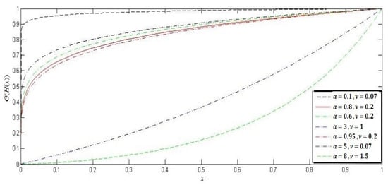
Figure 1. The CDF of APTPO distribution for different values of $\alpha$ and $\nu$.

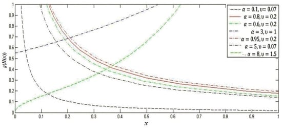
Figure 2. The PDF of APTPO distribution for different values of $\alpha$ and $\nu$.

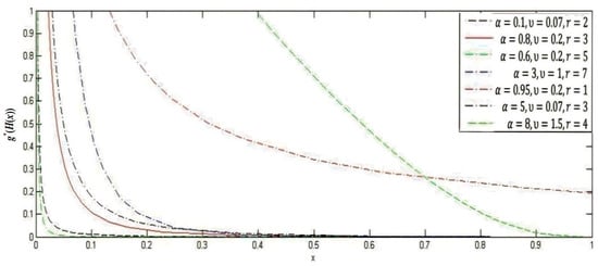
Figure 3. The APTPO PDF of the lower record values for different values of $\alpha$ and $\nu$ and r.

3. Estimating Parameters of the APTPO Probability Distribution Using Lower Record Values

In this section, we use lower record values to estimate the parameters of the APTPO probability distribution. Section 3.1 presents the derivation of the BLUE based on the r lower record values of the APTPO probability distribution. Section 3.2 details the derivation of the BLIE using the r-lower record values from the APTPO probability distribution. Section 3.3 focuses on the development of a prediction for future records.

3.1. Estimate Parameters of APTPO Distribution Using Best Linear Unbiased Estimates (BLUEs)

By applying Equation (11), the $n^{th}$ moment of $X_{L\left(r\right)}$ from the APTPO probability distribution is given as

$$E{\left(X_{L\left(r\right)}\right)}^n={\int }_0^1\frac{\nu log\left(\alpha \right)}{\Gamma \left(r\right)(\alpha -1)}{[-ln\left(\frac{{\alpha }^{x^{\nu }}-1}{\alpha -1}\right)]}^{r-1}{\alpha }^{x^{\nu }}{x}^{\nu +n-1}dx,n\ge 1$$

(12)

Let $e^y={\alpha }^{x^{\nu }},$ then,

$$E{\left(X_{L\left(r\right)}\right)}^n=\frac{{(log\left(\alpha \right))}^{\frac{-n}{\nu }}}{(\alpha -1)\Gamma \left(r\right)}{\int }_0^{log\left(\alpha \right)}{e}^y{y}^{\frac{n}{\nu }}{[-\ln \left(\frac{e^y-1}{\alpha -1}\right)]}^{r-1}dy$$

Let $z=e^y$, and we can obtain that

$$E{\left(X_{L\left(r\right)}\right)}^n=\frac{{(log\left(\alpha \right))}^{\frac{-n}{\nu }}}{(\alpha -1)\Gamma \left(r\right)}{\int }_1^{\alpha }{(logz)}^{\frac{n}{\nu }}{[-\ln \left(\frac{z-1}{\alpha -1}\right)]}^{r-1}dz$$

(13)

For $n=1$, we have

$$E\left(X_{L\left(r\right)}\right)=\theta 1_r$$

(14)

For $n=2$, we can calculate $E{\left(X_{L\left(r\right)}\right)}^2$, which helps in the calculation of

$$Var\left(X_{L\left(r\right)}\right)=\theta 1_r\theta 2_r$$

(15)

Consequently, for $s>r,x_s<x_r,$ we can calculate the covariance of $X_{L\left(r\right)}$ and $X_{L\left(s\right)}$ as follows:

$$Cov(X_{L\left(r\right)},X_{L\left(s\right)})=E\left(X_{L\left(r\right)}{X}_{L\left(s\right)}\right)-E\left(X_{L\left(r\right)}\right)E\left(X_{L\left(s\right)}\right)=\theta 1_s.\theta 2_r$$

(16)

By applying the following theorem, one can estimate the parameters of the APTPO probability distribution using lower record values:

Theorem 1.

Let $x_1,x_2,\dots ,x_r$ be r record values from the APTPO probability distribution (Equation (8)). Then, the best linear unbiased estimates (BLUE), denoted as $\widehat{\lambda }$ and $\widehat{\beta }$, for λ and β, respectively, are as follows:

$$\widehat{\lambda }=\frac{{\alpha }^{\prime }{V}^{-1}(\alpha 1^{\prime }-1{\alpha }^{\prime })V^{-1}h}{\Delta }$$

and

$$\widehat{\beta }=\frac{1^{\prime }{V}^{-1}(1{\alpha }^{\prime }-\alpha 1^{\prime })V^{-1}h}{\Delta }$$

where

$$h^{\prime }=(x_1,x_2,\dots ,x_r),$$

$${\alpha }^{\prime }=(\theta 1_1,\theta 1_2,\dots ,\theta 1_r),$$

$$V=\left({\upsilon }_{i}j\right),{\upsilon }_{i}j=\theta 2_i\theta 1_j,1\le i,j\le r,$$

$$\Delta =\left({\alpha }^{\prime }{V}^{-1}\alpha \right)\left(1^{\prime }{V}^{-1}1\right)-{\left({\alpha }^{\prime }{V}^{-1}1\right)}^2.$$

Proof. 

$$h^{\prime }=(x_1,x_2,\dots ,x_r),$$

then

$$E\left(h^{\prime }\right)=\mu 1+{\beta }^2\alpha ,$$

$$Var\left(h^{\prime }\right)={\beta }^{2}V$$

where, from Equations (13) and (16),

$$1^{\prime }=(1,1,\dots \dots ,1),$$

$${\alpha }^{\prime }=(\theta 1_1,\theta 1_2,\dots ,\theta 1_r)$$

$$V=\left({\upsilon }_{i}j\right),{\upsilon }_{ij}=\theta 2_i{b}_j,1\le i,j\le r,$$

$$V^{-1}=\left(V^{ij}\right),1\le i<j\le r.$$

Then, the entries of $V^{-1}$ are given by

$$V^{ii}=\frac{\theta 2_{i+1}\theta 1_{i-1}-\theta 2_{i-1}\theta 1_{i+1}}{(\theta 2_{i+1}\theta 1_{i-1}-\theta 2_{i-1}\theta 1_i)(\theta 2_{i+1}\theta 1_i-\theta 2_i\theta 1_{i+1})},i=1,\dots ,r-1,$$

$$V^{ij}=V^{ji}=\frac{-1}{\theta 2_{i+1}\theta 1_i-\theta 2_i\theta 1_{i+1}},j=i+1,i=1,2,\dots ,r-1$$

$$V^{ij}=0for|i-j|>1$$

$$V^{rr}=\frac{\theta 1_{r-1}}{\theta 1_r(\theta 2_r\theta 1_{r-1}-\theta 2_{r-1}\theta 1_r)},$$

$$\Delta =\left({\alpha }^{\prime }{V}^{-1}\alpha \right)\left(1^{\prime }{V}^{-1}1\right)-{\left({\alpha }^{\prime }{V}^{-1}1\right)}^2.$$

Applying the method introduced by Lioyd [15], the best linear unbiased estimates (BLUE), denoted as $\widehat{\lambda }$ and $\widehat{\beta }$, for $\lambda$ and $\beta$ based on r lower record values from the APTPO distribution, are given by

$$\widehat{\lambda }=\frac{{\alpha }^{\prime }{V}^{-1}(\alpha 1^{\prime }-1{\alpha }^{\prime })V^{-1}h}{\Delta }$$

and

$$\widehat{\beta }=\frac{1^{\prime }{V}^{-1}(1{\alpha }^{\prime }-\alpha 1^{\prime })V^{-1}h}{\Delta }$$

 □

The variance and covariance of $\widehat{\lambda },\widehat{\beta }$ are given by

$$Var\left(\widehat{\lambda }\right)=\frac{{\alpha }^{\prime }{V}^{-1}\lambda }{\Delta }{\beta }^2,$$

$$Var\left(\widehat{\beta }\right)=\frac{1^{\prime }{V}^{-1}1}{\Delta }{\beta }^2,$$

$$Cov(\widehat{\lambda },\widehat{\beta })=\frac{{\alpha }^{\prime }{V}^{-1}1}{\Delta }{\beta }^2,$$

By using the Matlab program (version 2021), the coefficients of the BLUEs for $\lambda ,\beta$ and variance-covariance for $\lambda$ and $\beta$ are given in Table 1 and Table 2, respectively.

Table 1. Coefficients for the BLUE of $\lambda$ and $\beta$ ($\nu =0.5,\alpha =1.5$).

n	r	The Coefficient for the BLUE of $\mathit{\lambda }$	The Coefficient for the BLUE of $\mathit{\beta }$
2	1	−0.561	4.247
2	2	1.561	−4.2479
3	1	−0.1014	2.997
3	2	−0.1654	0.45
3	3	1.2467	−3.4472
4	1	−0.0212	2.7789
4	2	−0.0346	0.0942
4	3	−0.158	0.43
4	4	1.2138	−3.3031
5	1	−0.0045	2.7335
5	2	−0.0074	0.0201
5	3	−0.0337	0.0916
5	4	−0.1557	0.4236
5	5	1.2012	−3.2688
6	1	−0.001	2.7238
6	2	−0.0016	0.0042
6	3	−0.0071	0.0193
6	4	−0.0327	0.089
6	5	−0.1584	0.04311
6	6	1.2007	−3.2679
7	1	−0.0002	2.7217
7	2	−0.0003	0.0009
7	3	−0.0015	0.0041
7	4	−0.0007	0.0188
7	5	−0.0334	0.0909
7	6	−0.1535	0.4177
7	7	1.1958	−3.2541
8	1	0	2.7213
8	2	−0.0001	0.0002
8	3	−0.0003	0.0008
8	4	−0.0014	0.0039
8	5	−0.007	0.019
8	6	−0.0321	0.0873
8	7	−0.1548	0.4212
8	8	1.1957	−3.2537
9	1	0	2.7212
9	2	0	0
9	3	−0.0001	0.0002
9	4	−0.0003	0.0008
9	5	−0.0014	0.0039
9	6	−0.0066	0.018
9	7	−0.0319	0.0869
9	8	−0.157	0.4273
9	9	1.1974	−3.2584
10	1	0	2.7212
10	2	0	0
10	3	0	0
10	4	−0.0001	0.002
10	5	−0.0003	0.0008
10	6	−0.0014	0.0037
10	7	−0.0066	0.0179
10	8	−0.0324	0.0881
10	9	−0.1552	0.4223
10	10	1.1959	−3.2543

Table 2. Coefficient for variance-covariance of the BLUE of $\lambda$ and $\beta$ in terms of ${\beta }^2$ ($\nu =0.5,\alpha =1.5$).

	$\mathit{r}$ = 2	$\mathit{r}$ = 3	$\mathit{r}$ = 4	$\mathit{r}$ = 5	$\mathit{r}$ = 6	$\mathit{r}$ = 7	$\mathit{r}$ = 8	$\mathit{r}$ = 9	$\mathit{r}$ = 10
1	0.0522	0.0094	0.002	0.0004	0.000009	0.00009	0	0	0
2	0.8417	1.1585	0.2137	1.2252	1.2277	1.2282	1.2283	1.2284	1.228
3	−0.1421	−0.0257	−0.0054	−0.0011	−0.00024	−0.0005	−0.00001	0	0

3.2. Best Linear Invariant Estimates (BLIEs)

The best linear invariant estimators (BLIE) $\tilde{\lambda },\tilde{\beta }$ of $\lambda$ and $\beta$ (in terms of minimum mean squared error and invariance with respect to the location parameter $\lambda$) are

$$\tilde{\lambda }=\widehat{\lambda }-\widehat{\beta }\left(\frac{E_{12}}{1+E_{22}}\right)$$

(17)

and

$$\tilde{\beta }=\frac{\widehat{\beta }}{1+E_{22}},$$

(18)

where $\widehat{\mu }$ and $\widehat{\beta }$ are BLUE of $\lambda$ and $\beta$, and

$$\left(\begin{array}{cc}Var\left(\widehat{\lambda }\right)& Cov(\widehat{\lambda },\widehat{\beta })\\ Cov(\widehat{\lambda },\widehat{\beta })& Var\left(\widehat{\beta }\right)\end{array}\right)={\widehat{\beta }}^2\left(\begin{array}{cc}{E}_{11}& E_{12}\\ E_{21}& E_{22}\end{array}\right)$$

The mean square errors of these estimators are

$$MSE\left(\tilde{\lambda }\right)={\widehat{\beta }}^2[E_{11}-\frac{E_{12}^2}{1+E_{22}}]$$

and

$$MSE\left(\tilde{\beta }\right)={\widehat{\beta }}^2\left[\frac{E_{22}^2}{1+E_{22}}\right]$$

3.3. Prediction of the Future Record

Finally, the concept for a specific phenomena that is probabilistically defined by the APTPO function probability distribution has been introduced in this paper. We generated some lower record value distributional features and achieved certain attributes that are important to this distribution. To predict future observations, this can be accomplished by utilizing return levels.

$$F\left(x_s\right)=1/s,s>r$$

which gives

$$x_s=\widehat{\lambda }+\widehat{\beta }{\left(\frac{ln[\alpha -1-s]}{ln\left(\alpha \right)}\right)}^{(1/\nu )}$$

(19)

4. The Maximum Likelihood Technique

Let $x_1,x_2,\dots ,x_n$ follow a completely random sampling from the APTPO distribution function (7). The records required for this investigation were obtained as follows: The first recording, $X_{L\left(1\right)}$, is $x_1$, so the first observation is $X_{L\left(1\right)}=x_1$. Observing the independently distributed random variables with the same distribution $X_i^{{}^{\prime }s}$ sequentially from $x_2,\dots x_n$ yields the second record value, $X_{L\left(2\right)}$. Let the next observation that is less than $X_{L\left(1\right)}$ need a number of trials to acquire $X_{L\left(2\right)}$ equal to $K_1$. For example, let the next observation that is less than $X_{L\left(1\right)}$ be $X_7$, so the number of trials to obtain $X_{L\left(2\right)}$ will be $K_1=6$.

Let $X_{L\left(1\right)}=x_1,K_1=k_1,X_{L\left(2\right)}=x_2,K_2=k_2\dots ,X_{L\left(r\right)}=x_r,K_r=k_r$, where $\{X_{L\left(i\right)},1\le i\le r\}$ is the record value sequence and $\{K_i,i>0\}$ and $k_r=1$ is the inter-record time sequence. Note that the number of records acquired $\left(r\right)$ will be smaller than n, the size of the entire random data sample, when this approach is used. It’s important to emphasize that the lower record values are the record numbers that do not include the inter-record times.

The likelihood function can be stated as

$$L(x,\mu ,\beta )=\prod _{i=1}^{r}f\left(x_i\right){[1-F\left(x_i\right)]}^{(k_i-1)}$$

For the record-breaking samples, let $X_{L\left(1\right)}=x_1,K_1=k_1,X_{L\left(2\right)}=x_2,K_2=k_2\dots ,X_{L\left(r\right)}=x_r,K_r=k_r$, where $f\left(x_i\right)$ and $F\left(x_i\right)$ are the PDF and CDF, respectively, of the random variable from which the record observations are obtained.

Applying the likelihood function to the record observations obtained from the APTPO distribution, we obtain that

$$L_1(x,\lambda ,\beta )=\prod _{i=1}^r\frac{\nu log\left(\alpha \right)}{\alpha -1}{z_i}^{\nu -1}{\alpha }^{\beta z_i^{\nu }}{[1-\frac{\alpha \beta z_i^{\nu }-1}{\alpha -1}]}^{k_i-1}$$

(20)

where, $z_i=\frac{x_i-\lambda }{\beta }$.

The log of the likelihood function is

$$\begin{array}{c}log{L}_1(x,\lambda ,\beta )=\sum _{i=1}^r\{log\left(\frac{\nu log\left(\alpha \right)}{\alpha -1}\right)+(\nu -1)\sum _{i=1}^{r}log\left(z_i\right)+\beta log\left(\alpha \right)\sum _{i=1}^r{z}_i^{\nu }\\ \\ +(k_i-1)\sum _{i=1}^{r}log\left[\frac{\alpha -\alpha \beta z_i^{\nu }}{\alpha -1}\right]\}\end{array}$$

(21)

By taking the partial derivative of Equation (21) with respect to $\lambda$ and $\beta$, we obtain the following equations:

$$\frac{\partial log{L}_1(x,\lambda ,\beta )}{\partial \lambda }=\sum _{i=1}^r\frac{\nu -1}{x_i-\lambda }-\nu log\left(\alpha \right)\sum _{i=1}^r{z}_i^{\nu -1}+\sum _{i=1}^r\frac{(k_i-1)\alpha \nu z_i^{\nu -1}}{\beta (\alpha -\alpha z_i^{\nu })},$$

(22)

$$\frac{\partial log{L}_1(x,\lambda ,\beta )}{\partial \beta }=\sum _{i=1}^r-\frac{\nu -1}{\beta }+log\left(\alpha \right)\sum _{i=1}^r{z}_i^{\nu }+\frac{\nu log\left(\alpha \right)}{\beta }\sum _{i=1}^r{z}_i^{\nu -1}+\frac{\alpha }{\beta }\sum _{i=1}^r\frac{(k_i-1)z_i^{\nu }}{\alpha -\alpha z_i^{\nu }}$$

(23)

The maximum likelihood estimators for $\mu$ and $\beta$ for the record samples are obtained by setting Equations (22) and (23) to zero.

The estimates of the parameters inherent in Equations (20) and (21) are obtained as follows for the complete sample $X_1,X_2,\dots ,X_n$.

We can write the log-likelihood from the APTPO probability density function, given by Equation (8), as follows:

$$log\left(L_2(x,\lambda ,\beta )\right)=\sum _{i=1}^r\{log\left(\frac{\nu log\left(\alpha \right)}{\alpha -1}\right)+(\nu -1)\sum _{i=1}^{n}log\left(z_i\right)+\beta log\left(\alpha \right)\sum _{i=1}^n{z}_i^{\nu }$$

(24)

By taking the partial derivative of (24) with respect to $\lambda$ and $\beta$, we obtain the following equations:

$$\frac{\partial log{L}_2(x,\lambda ,\beta )}{\partial \lambda }=\sum _{i=1}^r\frac{\nu -1}{x_i-\lambda }-\nu log\left(\alpha \right)\sum _{i=1}^r{z}_i^{\nu -1},$$

(25)

and

$$\frac{\partial log{L}_2(x,\lambda ,\beta )}{\partial \beta }=\sum _{i=1}^r-\frac{\nu -1}{\beta }+log\left(\alpha \right)\sum _{i=1}^r{z}_i^{\nu }+\frac{\nu log\left(\alpha \right)}{\beta }\sum _{i=1}^r{z}_i^{\nu -1}$$

(26)

The maximum likelihood estimators for $\mu$ and $\beta$ for the complete samples are obtained by setting Equations (25) and (26) to zero.

To estimate the approximate confidence intervals for the parameters of the APTPO distribution, one needs the $2\times 2$ observed information matrices for the record-breaking samples and complete sample, which are denoted by $I\left({\Theta }_1\right)$ and $I\left({\Theta }_2\right),$ where ${\Theta }_1=(\lambda ,\beta )$ and ${\Theta }_2=(\lambda ,\beta )$. Then, the $2\times 2$ total observed information matrix associated with the APTPO distribution for the record-breaking samples is given by $I\left({\Theta }_1\right)$, where their parameters are replaced by their $MLE’s$, where

$$I\left({\Theta }_1\right)=\left(\begin{array}{cc}{I}_{\lambda \lambda }& I_{\lambda \beta }\\ I_{\beta \beta }& I_{\beta \beta }\end{array}\right)$$

with

$$\frac{{\partial }^{2}log{L}_1(x,\lambda ,\beta )}{\partial {\lambda }^2}=\sum _{i=1}^r\frac{-\nu +1}{{(x_i-\lambda )}^2}+\frac{\nu (\nu -1)log\left(\alpha \right)}{\beta }\sum _{i=1}^r{z}_i^{\nu -2}$$

$$-\sum _{i=1}^r\frac{(k_i-1){\nu }^2{z}_i^{2(\nu -1)}}{{(1-\beta z_i^{\nu })}^2}-\sum _{i=1}^r\frac{(k_i-1)\nu (\nu -1)z_i^{\nu -2}}{(1-\beta z_i^{\nu })},$$

$$\frac{{\partial }^{2}log{L}_1(x,\lambda ,\beta )}{\partial \lambda \beta }=\sum _{i=1}^r-\frac{\nu (\nu -1)log\left(\alpha \right)z(\nu -1)}{\beta }-\sum _{i=1}^r\frac{\nu z_i^{\nu }(k_i-1)(\nu -1)}{(x-\lambda )({\beta }^2{z}_i^{2\nu }-2\beta z_i^{\nu }+1)}$$

$$\frac{{\partial }^{2}log{L}_1(x,\lambda ,\beta )}{\partial {\beta }^2}=\sum _{i=1}^r\frac{\nu -1}{{\beta }^2}+\sum _{i=1}^r-\frac{\nu (\nu -1)log\left(\alpha \right)z^{\nu }}{\beta }-\sum _{i=1}^r\frac{(k_i-1)(\nu -1)(z_i^{\nu }\nu -\beta z_i^{2\nu })}{\beta ({\beta }^2{z}_i^{2\nu }-2\beta z_i^{\nu }+1)}$$

The $2\times 2$ total observed information matrix associated with the APTPO distribution is given by $I\left({\Theta }_2\right),$ wherein the parameters are replaced by their $MLE’s$, where

$$I\left({\Theta }_2\right)=\left(\begin{array}{cc}{I}_{\lambda \lambda }& I_{\lambda \beta }\\ I_{\beta \lambda }& I_{\beta \beta }\end{array}\right)$$

with

$$\frac{{\partial }^{2}log{L}_2(x,\lambda ,\beta )}{\partial {\lambda }^2}=\sum _{i=1}^r\frac{-\nu +1}{{(x_i-\lambda )}^2}+\frac{\nu (\nu -1)log\left(\alpha \right)}{\beta }\sum _{i=1}^r{z}_i^{\nu -2}$$

$$\frac{{\partial }^{2}log{L}_2(x,\lambda ,\beta )}{\partial \lambda \beta }=\sum _{i=1}^r-\frac{\nu (\nu -1)log\left(\alpha \right)z(\nu -1)}{\beta }$$

$$\frac{{\partial }^{2}log{L}_2(x,\lambda ,\beta )}{\partial {\beta }^2}=\sum _{i=1}^r\frac{\nu -1}{{\beta }^2}+\sum _{i=1}^r\frac{\nu (\nu -1)log\left(\alpha \right)z(\nu -2)}{\beta }$$

Under standard regularity conditions, $({\Theta }_1-\widehat{{\Theta }_1})$ asymptotically follows the multivariate normal distribution $N_3(o,-I{\left(\widehat{{\Theta }_1}\right)}^{-1})$ and the asymptotic distribution of $({\Theta }_2-\widehat{{\Theta }_2})$ is $N_2(o,-I{\left(\widehat{{\Theta }_2}\right)}^{-1})$. These distributions can be utilized to construct approximate confidence intervals for the model parameters. Thus, denoting, for example, the total observed information matrix evaluated at $\widehat{{\Theta }_1}$, that is, $-I\left(\widehat{{\Theta }_1}\right)$, by $-\widehat{I}$, one would have the following approximate $100(1-\alpha )\%$ confidence intervals for the parameters of the APTPO distribution:

$$\widehat{\lambda }\pm z_{\frac{\alpha }{2}}\sqrt{{(-{\widehat{I}}^{-1})}_{\lambda \lambda }}\widehat{\beta }\pm z_{\frac{\alpha }{2}}\sqrt{{(-{\widehat{I}}^{-1})}_{\beta \beta }}$$

where $z_{\frac{\alpha }{2}}$ denotes the $100{(1-\frac{\alpha }{2})}^{th}$ percentile of the standard normal distribution.

Goodness of Fit Tests

The goodness of fit for a statistical model describes how well it matches a set of data. Goodness of fit measures are frequently used to characterize the discrepancy between actual values and values that would have been anticipated under the relevant model. When testing statistical hypotheses, such data can be used, for illustration, to check for residual normality and determine whether two samples were drawn from the same distribution. When applying an Akaike information criterion (AIC) (see Akaike [16]), this can be evaluated as follows:

$$AIC=-2log\left(L\right)+2K$$

(27)

where L is the likelihood of the function and K is the number of estimated parameters. Note that smaller values indicate a better model.

5. Simulation Study

The performance of the estimators established in the preceding section can be verified through the following simulation studies.

1. The APTPO distribution is used with $\lambda =20,\beta =1,\nu =0.5$, and $\alpha =1.5$ from a small random sample of size $n=20$ to serve as a model:

$$19.94,19.97,19.99,19.24,19.3114,19.916,19.881,19.84,19.8,19.38,19.996,19.755,19.697$$

$$19.64,19.58,19.08,19,19.52,19.16,19.94$$

Four record values can be collected from the given random sample, such as

$$x_i=19.94,19.24,19.08,19$$

$$k_i=3,11,1,1$$

We determined the $\lambda$ and $\beta$ estimation parameters for $r=1,2,3,$ and 4 by applying the BLUE and BLIE methods. The standard error for each case is calculated. Applying Equation (19) in each situation yields the prediction for the fifth future observation. The results are listed in Table 3.

Table 3. The result of the simulation.

	BLUE ($\widehat{\mathit{\theta }}$)	S.E ($\widehat{\mathit{\theta }}$)	BLIE ($\tilde{\mathit{\theta }}$)	S.E ($\tilde{\mathit{\theta }}$)
$\lambda$	18.959	0.1186	18.9697	0.3149
$\beta$	2.6692	2.9407	0.2767	2.5271
Prediction 5th observation	18.9797		19.041

On the other hand, applying the MLE method to estimate the parameters of the APTPO distribution (see Section 4) for complete data and using inter-record time $k_i$, along with applying the AIC method (Equation (27)), provides the results shown in Table 4. This table indicates that the value of AIC in the case of inter-record times is smaller than the value in the case of the complete sample. This implies that the use of inter-record times is preferable.

Table 4. The maximum likelihood estimates and statistical model for goodness of fit.

	$\widehat{\mathit{\lambda }}$	$\widehat{\mathit{\beta }}$	AIC
Complete sample	18.959	0.0011	18.959
Inter record times	2.6692	2.958	0.674

2. The APTPO distribution is used with $\lambda =50,\beta =1.5,\nu =0.5$, and $\alpha =2$ from a large random sample of size $n=50$ to serve as a model:

$$49.9815,49.4179,49.3826,49.6761,49.9952,49.9894,49.9599,49.2360,49.8097,49.8765,$$

$$48.8804,48.7138,49.5201,49.3467,49.9988,48.7558,49.6465,49.6161,49.4526,49.9312,$$

$$48.9214,48.6715,49.0818,49.9145,49.7851,49.7594,48.6289,49.5849,49.9464,49.8555,$$

$$49.1209,49.8332,49.0023,49.9716,48.5862,49.7048,49.0422,49.8962,48.9620,50,$$

$$49.1597,48.7976,48.8392,49.3103,49.2734,49.1981,48.5432,48.5000,49.7326,49.48674$$

Eleven record values can be collected from the given random sample, such as

$$x_i=49.9815,49.4179,49.3826,49.2360,48.8804,48.7558,48.6715,$$

$$48.6289,48.5862,48.5432,48.5000$$

$$k_i=1,1,1,5,3,5,6,5,8,12,1.$$

We determined the $\lambda$ and $\beta$ estimation parameters for $r=1,2,3,$ and 4 by applying the BLUE and BLIE methods. The standard error for each case is calculated. Applying Equation (19) in each situation yields the prediction for the 12th future observation. The results are listed in Table 5.

Table 5. The result of the simulation.

	BLUE ($\widehat{\mathit{\theta }}$)	S.E ($\widehat{\mathit{\theta }}$)	BLIE ($\tilde{\mathit{\theta }}$)	S.E ($\tilde{\mathit{\theta }}$)
$\lambda$	48.4893	0	48.4893	0.0035
$\beta$	−3.8069	15.8646	−0.2257	3.6924
Prediction 12th observation	48.4386		48.4863

On the other hand, applying the MLE method to estimate the parameters of the APTPO distribution (see Section 4) for complete data and using inter-record time $k_i$ provides the results shown in Table 6.

Table 6. The maximum likelihood estimates and statistical model for simulation.

	$\widehat{\mathit{\lambda }}$	$\widehat{\mathit{\beta }}$
Complete sample	48.5	2.7394
Inter record times	48.5755	0.4994

6. Real Life Example

The vinyl chloride data, obtained from clean upgrading monitoring wells in mg/L, were used by Bhaumik et al. [17]. The data set includes the following sample:

$$5.1,1.2,1.3,0.6,0.5,2.4,0.5,1.1,8.0,0.8,0.4,0.6,0.9,0.4,2.0,0.5,5.3,3.2,2.7,2.9,2.5,$$

$$2.3,1.0,0.2,0.1,0.1,1.8,0.9,2.0,4.0,6.8,1.2,0.4,0.2.$$

Idika et al. [14] proved that the data follow the APTPO distribution, yielding the smallest K-S statistic values and the largest K-S p-value (0.9602) with $\widehat{\nu }=2.021596$ and $\widehat{\alpha }=21.074041$. Seven record values can be collected from the given random sample, such as

$$x_i=5.1,1.2,0.6,0.5,0.4,0.2,0.1$$

$$k_i=1,1,2,1,6,13,1$$

We determined the $\lambda$ and $\beta$ estimation parameters for $r=1,2,3,4,5,6$, and 7 by applying the BLUE and BLIE methods. The standard error for each case is determined, and the results are listed in Table 7.

Table 7. The result of the estimation.

	BLUE ($\widehat{\mathit{\theta }}$)	S.E ($\widehat{\mathit{\theta }}$)	BLIE ($\tilde{\mathit{\theta }}$)	S.E ($\tilde{\mathit{\theta }}$)
$\lambda$	0.2265	0.1763	4.9421	−0.399
$\beta$	5.6408	0	8.2233	0

On the other hand, applying the MLE method to estimate the parameters of the APTPO distribution (see Section 4) for complete data and using inter-record time $k_i$, along with applying AIC method (Equation (27)), provides the results shown in Table 8. This table indicates that the value of AIC in the case of inter-record times is smaller than the value in the case of the complete sample. This means that using inter-record times is preferable.

Table 8. The maximum likelihood estimates and statistical model for goodness of fit.

	$\widehat{\mathit{\lambda }}$	$\widehat{\mathit{\beta }}$	AIC
Complete sample	5.0849	10.1106	−10.4665
Inter record times	5.1	−1.0381	−45.3494

7. Conclusions

In this study, we introduced the concept of records for a specific event described probabilistically by the APTPO PDF. We found the coefficients for the best linear unbiased estimates and the best linear invariant estimators. A method for forecasting future observations based on available data was also provided. The analytical framework for records and maximum probability estimates was established. Additionally, we calculated approximate confidence intervals for the parameters of the APTPO distribution. We used engaging classical applications to demonstrate the value of our analytical advancements. Furthermore, it was utilized to model a real-life scenario, serving as an explanatory tool to verify that our data fit the suggested distributions. Finally, the estimates from our study using inter-record times outperformed earlier findings.

References

- Chandler, K.M. The Distribution and Frequency of Record Values. J. R. Stat. Soc. Ser. B 1952, 14, 220–228. [Google Scholar] [CrossRef]
- Feller, W. An Introduction to Probability Theory and Its Application; John Wiley & Sons, Inc.: New York, NY, USA, 1965. [Google Scholar]
- Samaniego, F.J.; Whitaker, L.R. On Estimating Population Characteristics from Record-Breaking Observations. I. Parametric Results. Nav. Res. Logist. Q. 1986, 33, 531–543. [Google Scholar] [CrossRef]
- Gulati, S.; Padgett, W.J. Parametric and Nonparametric Inference from Record-Breaking Data; Springer: New York, NY, USA, 2003. [Google Scholar]
- Raul, G.; Javier, F.; Lina, M.; Gerardo, S. Statistical Inference for the Weibull Distribution Based on δ-Record Data. Symmetry 2019, 12, 20. [Google Scholar]
- Ahsanullah, M. Linear Prediction of Record Values for the Two Parameter Exponential Distribution. Ann. Inst. Stat. Math. 1980, 32, 363–368. [Google Scholar] [CrossRef]
- Nigm, E.M. Record Values from Inverse Weibull Distribution and Associated Inference. J. Appl. Stat. 2007, 16, 103–114. [Google Scholar]
- Johnson, N.L.; Kotz, S.; Balakrishnan, N. Continuous Univariate Distributions-I; John Wiley: New York, NY, USA, 1994. [Google Scholar]
- Mahadevi, A.; Kundu, D. A new method of generating distribution with an application to exponential distribution with an application to exponential distribution. Comm. Statist. Theory Methods 2017, 46, 6543–6557. [Google Scholar] [CrossRef]
- Mazen, N.; Ahmed, Z.A.; Mohammed, K.S. Estimation Methods of Alpha Power Exponential Distribution with applications to Engineering and Medical Data. Pak. J. Stat. Oper. Res. 2020, 16, 149–166. [Google Scholar]
- Refah, A.; Ahmed, E.; Hoda, R.; Mazen, N. Inferences for Alpha Power Exponential Distribution Using Adaptive Progressively Type-II Hybrid Censored Data with Applications. Symmetry 2022, 14, 651. [Google Scholar] [CrossRef]
- Fatehi, Y.E.; Chhaya, D.S. Alpha Power Transformed Extended power Lindley Distribution. J. Stat. Theory Appl. 2022, 22, 1–18. [Google Scholar]
- Luca, L. Combination of measurements and the BLUE method. In Proceedings of the 12th Quark Confinement, Thessaloniki, Greece, 28 August–4 September 2017; Volume 137, p. 106. [Google Scholar] [CrossRef]
- Idika, E.; Johnson Ohakweb, O.; Osuc, B.O.; Chris, U. Onyemachid α-Power transformed transformed power function distribution with applications. Heliyon 2021, 7, e08047. [Google Scholar]
- Lloyd, E.H. Least-squares estimation of location and scale parameters using order statistics. Biometrika 1952, 39, 88–95. [Google Scholar] [CrossRef]
- Akaike, H. A New Look at the Statistical Model Identification. IEEE Trans. Automat. Contr. 1974, 19, 716–723. [Google Scholar] [CrossRef]
- Bhaumik, D.K.; Kapur, K.; Gibbons, R.D. Testing Parameters of a Gamma Distribution for Small Samples. Technometrics 2009, 51, 326–334. [Google Scholar] [CrossRef]
Disclaimer/Publisher’s Note: The statements, opinions and data contained in all publications are solely those of the individual author(s) and contributor(s) and not of MDPI and/or the editor(s). MDPI and/or the editor(s) disclaim responsibility for any injury to people or property resulting from any ideas, methods, instructions or products referred to in the content. |
© 2023 by the authors. Licensee MDPI, Basel, Switzerland. This article is an open access article distributed under the terms and conditions of the Creative Commons Attribution (CC BY) license (https://creativecommons.org/licenses/by/4.0/).