Classical and Bayesian Inference for the Kavya–Manoharan Generalized Exponential Distribution under Generalized Progressively Hybrid Censored Data

Abstract

This manuscript focuses on the statistical inference of the Kavya–Manoharan generalized exponential distribution under the generalized type-I progressive hybrid censoring sample (GTI-PHCS). Different classical approaches of estimation, such as maximum likelihood, the maximum product of spacing, least squares (LS), weighted LS, and percentiles under GTI-PHCS, are investigated. Based on the squared error and linear exponential loss functions, the Bayes estimates for the unknown parameters utilizing separate gamma priors under GTI-PHCS have been derived. Point and interval estimates of unknown parameters are developed. We carry out a simulation using the Monte Carlo algorithm to show the performance of the inferential procedures. Finally, real-world data collection is examined for illustration purposes.

1. Introduction

Censoring schemes (CSs) play a significant role in lifespan and reliability studies. According to the estimated experiment time and accompanying cost, many practical experiments that rely on the lifespan of objects may be completed before failing all of the items. In these situations, just a subset of an item’s failure information is recorded, and the data collected is known as censored data.

The most popular censoring methods used in life tests are type-I and type-II CSs. Ref. [1] proposed a hybrid CS, which is a combination of type-I and type-II CSs. In many cases, it is prepared in advance to remove items prior to failure at several stages of the experiment; however, the above CS lack the flexibility to allow for items to be removed from the experiment at stages other than the trial’s endpoint. To address this issue, Ref. [2] proposed a type-II progressive CS (T-IIPCS) as a generalization for the censoring systems described previously.

The following can be used to establish T-IIPCS: Assume that a life-test experiment is conducted on a random sampling of n items and that the trial’s starting point is the number of reported failures $m(<n)$, which was previously progressive CS ($R_1,R_2,\dots ,R_m$). During the time of the smallest failure, $X_{1:n}$, $R_1$ operating items are picked at random and left out of the experiment. At the second lowest failure time $X_{2:n}$, $R_2$ operational items are randomly chosen and eliminated from the experiment. The procedure is continued until the final failure time $X_{m:n}$ takes place, at which point all remaining operational items $R_m=n-m-{\sum }_{i=1}^{m-1}{R}_i$ are removed from the experiment. The experiment is then terminated at $X_{m:n}$.

T-IIPCS has one big drawback in that if the items being studied are reliable and of excellent quality, the experiment time may be very long. This restriction was addressed in Ref. [3] with an improved system known as a type-I progressive hybrid CS (TI-PHCS), in which $n, m,$ and ($R_1,R_2,\dots ,R_m$), as well as the experimental duration $\tau$, is determined beforehand. In this case, the experiment is completed at time $X^{*}=$ min$\left\{X_{m:n},\tau \right\}$. Except for the last time point, this scheme is identical to T-IIPCS.

One of T-IIPHCS’s most significant shortcomings is that the effective sample size is random and might be relatively small. As a result, statistical inference techniques may be unreliable or less efficient. A novel variation of progressive censoring called the generalized TI-PHCS (GTI-PHCS) was introduced in Ref. [4] to eliminate the problems that emerged in TI-PHCS, in which a smaller number of failures is predetermined. Using this filtering method would save time and money throughout a lifetime test trial. Additionally, the experiment having more failures improves estimates of statistical efficacy. The CS aids in ensuring that at least a constant number of observed items $w(<m<n)$ are satisfied to attain the efficiency necessary for statistical evaluation. It also controls the experiment’s overall duration to be close to that time if the number of observed failures appears to be very low up until $\tau$. In this case, the experiment is completed at the moment $X^{*}=\max \{X_{w:n},\min \left\{X_{m:n},\tau \right\}\}$ and any remaining operational items are removed from the experiment.

Numerous researchers have reported different techniques of estimation using the GTI-PHCS. In accordance with maximum product spacing (MPS), Ref. [5] introduced progressive type-II hybrid CS. For an exponential (E) model and a Weibull model, respectively Refs. [4,6] provided an accurate likelihood inference and entropy estimation methodology. Salem et al. [7] discussed a joint Type-II generalized progressive hybrid censoring scheme based on exponential distribution. By combining the generalized E (GE) and the basic step-stress accelerated life test with the competing risks model Ref. [8] investigated the statistical prediction problem of unobserved failure durations. In Refs [9,10], Bayesian and maximum likelihood (ML) estimation strategies for the E and Weibull under competing risks models were examined. When applying partially accelerated life tests to units whose lives are exponentially distributed under normal stress circumstances, [11] explored several point and interval estimates for the parameters involved, as well as the ideal stress change time. Ref. [12] examined the competing risk models under GTI-PHCS based on Chen distribution. Ref. [13] used GTI-PHCS to estimate the Weibull distribution’s unknown parameters, reliability, and hazard functions with application to real data. Ref. [14] provided the ML and Bayesian estimators of the distribution’s parameters, together with the reliability and hazard functions, based on GTI-PHCS data, from a GE distribution with application to numbers of million revolutions data before failure for each of the 23 ball bearings in the life test.

The GE model has been shown to be beneficial in a wide range of applications involving life testing, survival analysis, and reliability. Ref. [15] investigated this model, which is a special instance of the exponentiated Weibull model [16,17]. The followings are the cumulative distribution function (CDF) and probability density function (PDF) of the GE model, with scale parameter $\lambda$ and shape parameter $\theta$, for $x>0$:

$$G(x;\theta ,\lambda )={(1-e^{-\lambda x})}^{\theta },\hspace{1em}\theta ,\lambda >0,$$

(1)

$$g(x;\theta ,\lambda )=\lambda \theta e^{-\lambda x}{\left(1-e^{-\lambda x}\right)}^{\theta -1}.$$

(2)

Several authors used the PDF (2) and CDF (1) to generate new extensions of the GE model, such as beta GE model [18], Marshall–Olkin GE [19], half-Cauchy GE [20], odd Lomax GE [21], and modified slashed GE [22]. Recently, [23] introduced the Kavya–Manoharan GE (KMGE) model as the special case of the Kavya–Manoharan exponentiated Weibull model. The KMGE distribution is a new extension where it does not require any additional parameters to the baseline distribution which absolutely is an advantage with no more parameters. The CDF, PDF, and hazard rate function (HRF) of the KMGE model are

$$F(x;\theta ,\lambda )=\frac{e}{e-1}\left[1-e^{-{\left(1-e^{-\lambda x}\right)}^{\theta }}\right],x>0,\theta ,\lambda >0,$$

(3)

$$f(x;\theta ,\lambda )=\frac{e}{e-1}\lambda \theta e^{-\lambda x}{\left(1-e^{-\lambda x}\right)}^{\theta -1}{e}^{-{\left(1-e^{-\lambda x}\right)}^{\theta }},$$

(4)

and

$$h(x;\theta ,\lambda )=\frac{e\lambda \theta e^{-\lambda x}{\left(1-e^{-\lambda x}\right)}^{\theta -1}{e}^{-{\left(1-e^{-\lambda x}\right)}^{\theta }}}{e^{-{\left(1-e^{-\lambda x}\right)}^{\theta }}-1}.$$

The plots of these PDF and HRF are displayed in Figure 1. It can be noticed from this figure that the PDF can be uni-modal, decreasing, and right-skewed, but the HRF can be increasing, decreasing, and constant. These curves indicate that the KMGE model is very flexible in modeling different types of data.

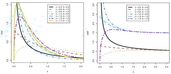
Figure 1. Plots of the PDF and HRF of the KMGE model.

As far as we are aware, there has not been any research that uses MPS, LS, and weighted LS (WLS) estimation techniques to estimate model parameters of probability distribution in the presence of the GTI-PHC data. Then according to the novelty of the KMGE distribution, we provide three important estimation methods besides the ML, percentiles (PE), and Bayesian methods. After that, a medical and engineering data application is supplied in accordance with the flexibility of the KMGE distribution (see Figure 1). In this regard, we summarized our study’s objectives as follows:

• Discuss the point and interval statistical inference of the two unknown parameters $\theta$ and $\lambda$ for the KMGE distribution using five classical estimation approaches such as ML, MPS, LS, WLS, and PE based on GTI-PHCS.
• Estimate the model’s parameters of the KMGE distribution in view of the Bayesian estimation strategy using symmetric and asymmetric loss functions.
• Using specific metrics of accuracy, a simulation study is run to look at how different estimates behave.
• A potential application based on GTI-PHCS has been explored for data from engineering and medical sciences.

The rest of this paper is structured as follows: the model formulation of GTI-PHCS is proposed in the Section 2. Five classical estimation approaches such as ML, MPS, LS, WLS, and PE are investigated in the Section 3. Bayesian estimation with credible intervals is discussed in the Section 4. In Section 5, we evaluate the quality points and interval estimators using a Monte Carlo approach. In Section 6, we employ the theoretical study findings to real-world data. Finally, the discussion and conclusion are presented in Section 7.

2. Generalized Type-I Progressive Hybrid Censoring

The implementation steps of the GTI-PHCS are described below:

• Assume that a random sample of n units undergoes a lifetime testing trial.
• Suppose that $X_1,X_2,\dots ,X_n$, have the KMGE model with CDF (3) and PDF (4).
• Assume that before starting the experiment, the integers $w,m$, the experimental time $\tau$ and ($R_1,R_2,\dots ,R_m$) are assigned, so that $0<\tau <\infty$, $0<w<m\le n$.
• The operational units $R_1$ are chosen at random and eliminated from the experiment at $X_{1:n}$, the first failure time. At the subsequent failure time $X_{2:n}$, $R_2$ operating units are randomly selected and eliminated from the experiment, and the procedure is repeated. Eventually, the experiment is completed when $X^{*}=\max \{X_{w:n},\min \left\{X_{m:n},\tau \right\}\}$, and any remaining operational units $R_{\mathcal{C}}$ are omitted from the experiment. Table 1 contains the values of the final censoring number $R_{\mathcal{C}}$.
  Table 1. Values of $X^{*}$, $\mathcal{K}$, $ϵ$, and $R_{\mathcal{C}}$, for three cases.

  	Case I	Case II	Case III
  $X^{*}$	$X_{w:n}$	$\tau$	$X_{m:n}$
  $\mathcal{K}$	w	$\mathfrak{B}$	m
  $ϵ$	0	1	0
  $R_{\mathcal{C}}$	$R_w=R_w^{*}=n-w-{\sum }_{i=1}^{w-1}{R}_i,$	$R_{\tau }^{*}=n-\mathfrak{B}-{\sum }_{i=1}^{\mathfrak{B}}{R}_i$	$R_m=n-m-{\sum }_{i=1}^{m-1}{R}_i$
  	${\sum }_{i=\mathfrak{B}+1}^{w-1}{R}_i=0$

• Assume that $\mathfrak{B}$ represents the number of units that fail prior to $\tau$. The experiment’s end time $X^{*}$ is, therefore, provided by

  $$X^{*}=\left\{\begin{array}{cc}{X}_{w:m:n},\hfill & \mathrm{if}\tau \le X_{w:m:n}<X_{m:m:n},\\ \tau ,\hfill & \mathrm{if}{X}_{w:m:n}\le \tau <X_{m:m:n},\\ X_{m:m:n},\hfill & \mathrm{if}{X}_{w:m:n}<X_{m:m:n}\le \tau .\end{array}\right.$$
  Any one of the subsequent six cases could be observed for the results:
  • Case I: If the observed time $\tau$ happens to occur before the wth failure time $X_{w:n}$ and $\mathfrak{B}(<w)$ failures occur up to time $\tau$, $\tau <X_{w:n}<X_{m:n}$. Afterward, we won’t remove any operating units from the experiment until the $(\mathfrak{B}+1)\mathrm{th},\dots ,(w-1)\mathrm{th}$ failure times, after which we will remove all of the remaining operating units $R_w^{*}=n-w-{\sum }_{i=1}^{w-1}{R}_i$ from the experiment at the wth failure time, thereby stopping the experiment at $X^{*}=X_{w:n}$, where $R_{\mathfrak{B}+1}=\cdots =R_{w-1}=0$, see Figure 2. In this case, we allow the experiment to continue after experimental time $\tau$ is reached to guarantee that at least the wth failure time $X_{w:n}$ happens. The following remarks, in this case, will be made: $X_{1:n}<\cdots <X_{\mathfrak{B}:n}\le \tau <X_{\mathfrak{B}+1:n}<\cdots <X_{w:n}.$
    

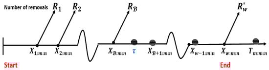    Figure 2. Case 1. The sampling process under GTI-PHCS, when $\tau <X_{w:n}<X_{m:n}$.
  • Case II: When wth failure time $X_{w:n}$ happens before the $\tau$, $X_{w:n}\le \tau <X_{m:n}$, and $\mathfrak{B}(\ge w)$ failures occur up to the $\tau$ time. The experiment is terminated at $X^{*}=\tau$ by removing all of the remaining operational units $R_{\tau }^{*}=n-\mathfrak{B}-{\sum }_{i=1}^{\mathfrak{B}}{R}_i$, as shown in Figure 3. The following observations will be made in this situation: $X_{1:n}<\cdots <X_{w:n}<\cdots <X_{\mathfrak{B}:n}\le \tau$.
    

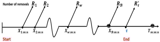    Figure 3. Case 2. The sampling process under GTI-PHCS, when $X_{w:n}\le \tau <X_{m:n}$.
  • Case III: When the mth failure time $X_{m:n}$ happens before the time $\tau$, $X_{w:n}<X_{m:n}\le \tau$, then all the remaining operational units $R_m=n-m-{\sum }_{i=1}^{m-1}{R}_i$ are deleted from the experiment, terminating it at $X^{*}=X_{m:n}$, as shown in Figure 4. The following observations will be made in this situation: $X_{1:n}<\cdots <X_{w:n}<\cdots <X_{m:n}\le \tau .$
    

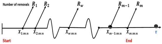    Figure 4. Case 3. The sampling process under GTI-PHCS, when $X_{w:n}<X_{m:n}\le \tau$.

3. Different Classical Approaches of Estimation

This section discusses five classical methods for calculating ML, MPS, LS, WLS, and PE of the underlying parameters $\theta$ and $\lambda$ using data gathered via GTI-PHCS.

3.1. Approach of ML Estimation

The likelihood function based on GTI-PHCS is provided via

$$\begin{array}{cc}\hfill \mathbf{L}(\theta ,\lambda ;\mathbf{x})\propto & \left[\prod _{j=1}^{\mathcal{K}}f\left(x_{j:n}\right){\left[1-F\left(x_{j:n}\right)\right]}^{R_j}\right]{[1-F(\tau \left)\right]}^{ϵR_{\tau }^{*}},\hfill \end{array}$$

(5)

where $\mathbf{x}$ = $(x_{1:n},\dots ,$ $x_{\mathcal{K}:n})$, $R_{\tau }^{*}=n-\mathcal{K}-{\sum }_{i=1}^{\mathcal{K}}{R}_i$, final censored number $R_{\mathcal{C}}$, and $X^{*}$, $\mathcal{K}$, $ϵ$ be experiment end time values based on three cases are reported in Table 1. It is interesting to note that, in Case I, several values of $R_i$, $i=1,2,\dots ,m$ may be different throughout the test than those set before the test even starts.

Utilizing CDF (3) and PDF (4), the log-likelihood function takes the below formula:

$$\begin{array}{cc}\hfill \mathcal{L}=log\mathbf{L}(\theta ,\lambda ;\mathbf{x})& \propto \mathcal{K}log\left[\lambda \theta \right]+\sum _{j=1}^{\mathcal{K}}\{-\lambda x_j+(\theta -1)log\left[1-e^{-\lambda x_j}\right]-{\left(1-e^{-\lambda x_j}\right)}^{\theta }\hfill \\ \hfill & +R_j\left(log\left[e^{1-{\left(1-e^{-\lambda x_j}\right)}^{\theta }}-1\right]\right)+ϵR_{\tau }^{*}\left(log\left[e^{1-{\left(1-e^{-\lambda \tau }\right)}^{\theta }}-1\right]\right)\}.\hfill \end{array}$$

(6)

Note that, we write $x_j$ instead of $x_{j:n}$ for the simplified form. According to Equation (6), $(\widehat{\theta },\widehat{\lambda })$ of $(\theta ,\lambda )$, can be computed as below: The ML estimates (MLEs) of $\theta$ and $\lambda$ may be determined by taking the first partial derivatives of (6) with regard to $\theta$ and $\lambda$ and equating them to zero as

$$\begin{array}{cc}\hfill \frac{\partial \mathcal{L}}{\partial \theta }=& \sum _{j=1}^{\mathcal{K}}\left\{\left(1-{\left(1-e^{-\lambda x_j}\right)}^{\theta }\right)log\left[1-e^{-\lambda x_j}\right]-R_j\left(\frac{{\left(1-e^{-\lambda x_j}\right)}^{\theta }log\left[1-e^{-\lambda x_j}\right]}{1-e^{{\left(1-e^{-\lambda x_j}\right)}^{\theta }-1}}\right)\right\}\hfill \\ & -ϵR_{\tau }^{*}\left(\frac{{\left(1-e^{-\lambda \tau }\right)}^{\theta }log\left[1-e^{-\lambda \tau }\right]}{1-e^{{\left(1-e^{-\lambda \tau }\right)}^{\theta }-1}}\right)+\frac{\mathcal{K}}{\theta }=0,\hfill \end{array}$$

$$\begin{array}{cc}\hfill \frac{\partial \mathcal{L}}{\partial \lambda }=& \sum _{j=1}^{\mathcal{K}}\left\{-x_j+\frac{x_j{e}^{-\lambda x_j}}{1-e^{-\lambda x_j}}\left(\theta -\theta {\left(1-e^{-\lambda x_j}\right)}^{\theta }-1\right)-R_j\left(\frac{\theta x_j{e}^{-\lambda x_j}{\left(1-e^{-\lambda x_j}\right)}^{\theta -1}}{1-e^{{\left(1-e^{-\lambda x_j}\right)}^{\theta }-1}}\right)\right\}\hfill \\ & -ϵR_{\tau }^{*}\left(\frac{\theta \tau e^{-\lambda \tau }{\left(1-e^{-\lambda \tau }\right)}^{\theta -1}}{1-e^{{\left(1-e^{-\lambda \tau }\right)}^{\theta }-1}}\right)+\frac{\mathcal{K}}{\lambda }=0.\hfill \end{array}$$

The MLEs $\widehat{\theta }$ and $\widehat{\lambda }$ of $\theta$ and $\lambda$ may be computed by solving the score equations, ${\displaystyle \frac{\partial \mathcal{L}}{\partial \theta }=0}$ and ${\displaystyle \frac{\partial \mathcal{L}}{\partial \lambda }=0}$, with regards to $\theta$ and $\lambda$ and solving these equations concurrently to produce the MLEs. Because analytical solutions cannot get the roots, these equations can indeed be investigated numerically utilizing iterative procedures employing statistical software via the “maxLik” package installed through the R 4.3.0 programming language.

According to the usual asymptotic normality theory of MLEs, we may assume that ${\displaystyle \frac{\widehat{\theta }-\theta }{\sqrt{\mathrm{V}\left(\widehat{\theta }\right)}}}$ and ${\displaystyle \frac{\widehat{\lambda }-\lambda }{\sqrt{\mathrm{V}\left(\widehat{\lambda }\right)}}}$ can be approximated by

$${\displaystyle \frac{\widehat{\theta }-\theta }{\sqrt{\mathrm{V}\left(\widehat{\theta }\right)}}\sim N(0,1)\mathrm{and}\frac{\widehat{\lambda }-\lambda }{\sqrt{\mathrm{V}\left(\widehat{\lambda }\right)}}\sim N(0,1),}$$

where $\mathrm{V}\left(\widehat{\theta }\right)$ and $\mathrm{V}\left(\widehat{\lambda }\right)$ are the variance of $\widehat{\theta }$ and $\widehat{\lambda }$ which may be founded by computing the inverse of the Fisher information matrix, i.e.,

$$\begin{array}{cc}\hfill \mathbf{I}\begin{array}{cc}\hfill =-& {\left(\begin{array}{cc}{\displaystyle \frac{{\partial }^2\pounds }{\partial {\theta }^2}}& {\displaystyle \frac{{\partial }^2\pounds }{\partial \theta \partial \lambda }}\\ {\displaystyle \frac{{\partial }^2\pounds }{\partial \lambda \partial \theta }}& {\displaystyle \frac{{\partial }^2\pounds }{\partial {\lambda }^2}}\end{array}\right)}_{\theta =\widehat{\theta },\lambda =\widehat{\lambda }}^{-1}\hfill \end{array}=& \left(\begin{array}{cc}\mathrm{V}\left(\widehat{\theta }\right)& \mathrm{Cov}(\widehat{\theta },\widehat{\lambda })\\ \mathrm{Cov}(\widehat{\theta },\widehat{\lambda })& \mathrm{V}\left(\widehat{\lambda }\right)\end{array}\right),\hfill \end{array}$$

(7)

where the caret $\widehat{}$ denotes that the derivative is evaluated at $(\widehat{\theta },\widehat{\lambda })$. It is simple to obtain the second partial derivatives of the probability function’s natural logarithm for $\theta$ and $\lambda$.

Suppose that ${\eta }_1=\theta$ and ${\eta }_2=\lambda$, then, a $100(1-\alpha )\%$ normal approximation confidence interval (NACI) of ${\eta }_i$, for $i=1,2$, may be easily computed as below:

$$\left(\max \{0,\widehat{{\eta }_i}-z_{\alpha /2}\sqrt{\mathrm{V}\left(\widehat{{\eta }_i}\right)}\},\widehat{{\eta }_i}+z_{\alpha /2}\sqrt{\mathrm{V}\left(\widehat{{\eta }_i}\right)}\right),$$

where $z_{\alpha /2}$ is the upper $\alpha /2$ percentile of $N(0,1)$ distribution, and $\widehat{{\eta }_i}$ is the MLE of ${\eta }_i$.

In the lower bound of NACI, as $n\to$∞, the positive parameter can occasionally have a negative value. Ref. [24], as $n\to$∞, recommended using a log transformation confidence interval (LTCI) in this situation. Based on the log-transformed MLE’s usual estimate, ${\displaystyle \frac{log\widehat{{\eta }_i}-log{\eta }_i}{\sqrt{\mathrm{V}(log\widehat{{\eta }_i})}}}$, where $i=1,2$, as a standard normal distribution can be approximated.

$${\displaystyle \mathrm{as}n\to \infty ,\frac{log\widehat{{\eta }_i}-log{\eta }_i}{\sqrt{\mathrm{V}(log\widehat{{\eta }_i})}}\sim N(0,1),}$$

where ${\displaystyle \mathrm{V}(log\widehat{{\eta }_i})=\frac{\mathrm{V}\left(\widehat{{\eta }_i}\right)}{{\widehat{{\eta }_i}}^2}}$. Accordingly, a $100(1-\alpha )\%$ LTCI for ${\eta }_i$ is characterized

$$\mathrm{as}n\to \infty ,\left(\widehat{{\eta }_i}exp\left[-{\displaystyle z_{\alpha /2}\frac{\sqrt{\mathrm{V}\left(\widehat{{\eta }_i}\right)}}{\widehat{{\eta }_i}}}\right],\widehat{{\eta }_i}exp\left[{\displaystyle z_{\alpha /2}\frac{\sqrt{\mathrm{V}\left(\widehat{{\eta }_i}\right)}}{\widehat{{\eta }_i}}}\right]\right).$$

3.2. Approach of Maximum Product of Spacing Estimation

Ref. [25] proposed an alternate technique to the ML method for estimating unknown parameters in continuous distributions. Refs. [26,27] utilized progressive type-II censoring to estimate the parameters involved in the Weibull and Kavya–Manoharan inverse length biased exponential distributions. The MPS estimates (MPSEs) are yielded by maximizing the next product of spacing for $\theta$ and $\lambda$.

$$\begin{array}{cc}\hfill \mathcal{P}(\theta ,\lambda ;\mathbf{x})& =\left(\prod _{j=1}^{\mathcal{K}+1}\left[F\left(x_j\right)-F\left(x_{j-1}\right)\right]\right)\left(\prod _{j=1}^{\mathcal{K}}{\left[1-F\left(x_j\right)\right]}^{R_j}\right){\left[1-F\left(\tau \right)\right]}^{ϵR_{\tau }^{*}},\hfill \end{array}$$

(8)

where $F\left(x_0\right)=0$ and $F\left(x_{\mathcal{K}+1}\right)=1$, and the expression about GTI-PHCS model has been discussed in Table 1. Utilizing (3) and by maximizing the product of spacing for $\theta$ and $\lambda$, then the MPSEs $\tilde{\theta }$ and $\tilde{\lambda }$ of $\theta$ and $\lambda$ are provided

$$\begin{array}{cc}\hfill \mathcal{P}(\theta ,\lambda ;\mathbf{x})& =a^{*}\left(1-e^{-{\left(1-e^{-\lambda x_1}\right)}^{\theta }}\right)\left(e^{1-{\left(1-e^{\lambda x_{\mathcal{K}}}\right)}^{\theta }}-1\right){\left[\frac{e^{1-{\left(1-e^{-\lambda \tau }\right)}^{\theta }}-1}{e-1}\right]}^{ϵR_{\tau }^{*}}\hfill \\ \hfill & \times \left(\prod _{j=2}^{\mathcal{K}}\left[e^{-{\left(1-e^{-\lambda x_{j-1}}\right)}^{\theta }}-e^{-{\left(1-e^{-\lambda x_j}\right)}^{\theta }}\right]\right)\left(\prod _{j=1}^{\mathcal{K}}{\left[\frac{e^{1-{\left(1-e^{-\lambda x_j}\right)}^{\theta }}-1}{e-1}\right]}^{R_j}\right),\hfill \end{array}$$

(9)

where $a^{*}=\frac{1}{e-1}{\left(\frac{e}{e-1}\right)}^{\mathcal{K}}$.

To obtain the MPSEs, the nonlinear equations can also be solved simultaneously. Since an exact solution cannot obtain the roots, these equations are analytically resolved using iterative strategies and statistical software:

$$\begin{array}{cc}\hfill \frac{\partial log\left[\mathcal{P}\right(\theta ,\lambda ;\mathbf{x}\left)\right]}{\partial \theta }& =\frac{A\left(x_1\right)}{1-D\left(x_1\right)}-\frac{A\left(x_{\mathcal{K}}\right)}{D\left(x_{\mathcal{K}}\right)-e^{-1}}-ϵR_{\tau }^{*}\frac{A\left(\tau \right)}{D\left(\tau \right)-e^{-1}}+\sum _{j=2}^{\mathcal{K}}\left[\frac{A\left(x_j\right)-A\left(x_{j-1}\right)}{D\left(x_{j-1}\right)-D\left(x_j\right)}\right]\hfill \\ & -\sum _{j=1}^{\mathcal{K}}\left[R_j\frac{A\left(x_j\right)}{D\left(x_j\right)-e^{-1}}\right]=0,\hfill \end{array}$$

$$\begin{array}{cc}\hfill \frac{\partial log\left[\mathcal{P}\right(\theta ,\lambda ;\mathbf{x}\left)\right]}{\partial \lambda }& =\frac{B\left(x_1\right)}{1-D\left(x_1\right)}-\frac{B\left(x_{\mathcal{K}}\right)}{D\left(x_{\mathcal{K}}\right)-e^{-1}}-ϵR_{\tau }^{*}\frac{B\left(\tau \right)}{D\left(\tau \right)-e^{-1}}+\sum _{j=2}^{\mathcal{K}}\left[\frac{B\left(x_j\right)-B\left(x_{j-1}\right)}{D\left(x_{j-1}\right)-D\left(x_j\right)}\right]\hfill \\ & -\sum _{j=1}^{\mathcal{K}}\left[R_j\frac{B\left(x_j\right)}{D\left(x_j\right)-e^{-1}}\right]=0,\hfill \end{array}$$

where

$$\begin{array}{cc}\hfill A\left(x_j\right)& =log\left[1-e^{-\lambda x_j}\right]{\left(1-e^{-\lambda x_j}\right)}^{\theta }{e}^{-{\left(1-e^{-\lambda x_j}\right)}^{\theta }},\hfill \end{array}$$

(10)

$$\begin{array}{cc}\hfill B\left(x_j\right)& =x_j\theta e^{-\lambda x_j}{\left(1-e^{-\lambda x_j}\right)}^{\theta -1}{e}^{-{\left(1-e^{-\lambda x_j}\right)}^{\theta }},\hfill \end{array}$$

(11)

$$\begin{array}{cc}\hfill D\left(x_j\right)& =e^{-{\left(1-e^{-\lambda x_j}\right)}^{\theta }},\hfill \end{array}$$

the same forms are provided for $j=1$, or $\mathcal{K}$.

3.3. Approaches of LS and WLS

Ref. [28] established the LS and WLS techniques for estimating the parameters of the beta distribution. Refs. [29,30] employed progressive type-II censoring to estimate the parameters contained in the doubly Poisson-exponential and exponential-doubly Poisson distributions. To estimate the parameters in the Poisson-logarithmic half-logistic distribution under a progressive-stress accelerated life test, Ref. [31] proposed adaptive type-II progressive hybrid censoring.

Let ($X_1,\dots ,X_{\mathcal{K}}$) be the ordered GTI-PHCS sample from the KMGE model of size $\mathcal{K}$. The LS estimates (LSEs) of $\lambda ,$ $\theta$ are derived by minimizing the below formula

$$\mathcal{S}(\theta ,\lambda )=\sum _{j=1}^{\mathcal{K}}{\left(F\left(x_j\right)-\mathrm{E}\left[\widehat{F}\left(x_j\right)\right]\right)}^2,$$

in which E$\left[\widehat{F}\left(x_j\right)\right]$ denotes the empirical CDF expectation, as supplied in [32]

$$\begin{array}{cc}\hfill \mathrm{E}\left[\widehat{F}\left(x_j\right)\right]& =1-\prod _{\nu =\mathcal{K}-j+1}^{\mathcal{K}}\left[{\displaystyle \frac{\nu +{\sum }_{i=\mathcal{K}-\nu +1}^{\mathcal{K}}{R}_i}{1+\nu +{\sum }_{i=\mathcal{K}-\nu +1}^{\mathcal{K}}{R}_i}}\right],j=1,\cdots ,\mathcal{K},\hfill \end{array}$$

As a result, the LSEs $\breve{\theta }$ and $\breve{\lambda }$ of $\theta$ and $\lambda$ are yielded by minimizing the following formula

$$\mathcal{S}(\theta ,\lambda )=\sum _{j=1}^{\mathcal{K}}{\left(\frac{e}{e-1}\left[1-e^{-{\left(1-e^{-\lambda x_j}\right)}^{\theta }}\right]-\mathrm{E}\left[\widehat{F}\left(x_j\right)\right]\right)}^2.$$

These estimates can also be achieved by simultaneously solving the nonlinear equations to generate the LSEs. These equations can be resolved analytically using iterative methods and statistical tools since precise solutions cannot get the roots.

$$\begin{array}{cc}\hfill \frac{\partial \mathcal{S}(\theta ,\lambda )}{\partial \theta }& =\sum _{j=1}^{\mathcal{K}}A\left(x_j\right)\left(\frac{e}{e-1}\left[1-e^{-{\left(1-e^{-\lambda x_j}\right)}^{\theta }}\right]-\mathrm{E}\left[\widehat{F}\left(x_j\right)\right]\right)=0,\hfill \end{array}$$

$$\begin{array}{cc}\hfill \frac{\partial \mathcal{S}(\theta ,\lambda )}{\partial \lambda }& =\sum _{j=1}^{\mathcal{K}}B\left(x_j\right)\left(\frac{e}{e-1}\left[1-e^{-{\left(1-e^{-\lambda x_j}\right)}^{\theta }}\right]-\mathrm{E}\left[\widehat{F}\left(x_j\right)\right]\right)=0,\hfill \end{array}$$

where $A\left(x_j\right)$ and $B\left(x_j\right)$ are provided in (10) and (11), respectively.

The WLS estimates (WLSEs) of $\theta$ and $\lambda$ may be generated by minimizing the below formula

$${\mathcal{S}}^{*}(\theta ,\lambda )=\sum _{j=1}^{\mathcal{K}}{\mathcal{W}}_j{\left(F\left(x_j\right)-\mathrm{E}\left[\widehat{F}\left(x_j\right)\right]\right)}^2,$$

where ${\displaystyle {\mathcal{W}}_j=\frac{1}{\mathrm{V}\left[\widehat{F}\left(x_j\right)\right]}}$ is the weight factor and $\mathrm{V}\left[\widehat{F}\left(x_j\right)\right]$ is the variance of the empirical CDF, see [32], which is provided via

$$\begin{array}{cc}\hfill \mathrm{V}\left[\widehat{F}\left(x_j\right)\right]& =\left(\prod _{\nu =\mathcal{K}-j+1}^{\mathcal{K}}{\Delta }_{\nu }\right)\left(\prod _{\nu =\mathcal{K}-j+1}^{\mathcal{K}}{\mathsf{\Omega }}_{\nu }-\prod _{\nu =\mathcal{K}-j+1}^{\mathcal{K}}{\Delta }_{\nu }\right),j=1,\dots ,\mathcal{K},\hfill \end{array}$$

where

$$\begin{array}{cc}\hfill {\Delta }_{\nu }& =\frac{\nu +{\sum }_{i=\mathcal{K}-\nu +1}^{\mathcal{K}}{R}_i}{1+\nu +{\sum }_{i=\mathcal{K}-\nu +1}^{\mathcal{K}}{R}_i},\nu =1,\dots ,\mathcal{K},\hfill \\ \hfill {\mathsf{\Omega }}_{\nu }& ={\Delta }_{\nu }+\frac{1}{(1+\nu +{\sum }_{i=\mathcal{K}-\nu +1}^{\mathcal{K}}{R}_i)(2+\nu +{\sum }_{i=\mathcal{K}-\nu +1}^{\mathcal{K}}{R}_i)},\nu =1,\dots ,\mathcal{K}.\hfill \end{array}$$

Minimizing the next quantity, we get the WLSEs $\ddot{\theta }$ and $\ddot{\lambda }$ of $\theta$ and $\lambda$.

$${\mathcal{S}}^{*}(\theta ,\lambda )=\sum _{j=1}^{\mathcal{K}}{\mathcal{W}}_j{\left(\frac{e}{e-1}\left[1-e^{-{\left(1-e^{-\lambda x_j}\right)}^{\theta }}\right]-\mathrm{E}\left[\widehat{F}\left(x_j\right)\right]\right)}^2.$$

To produce the WLSEs, the following nonlinear equations can be numerically solved via iterative methods and statistical tools:

$$\begin{array}{cc}\hfill \frac{\partial {\mathcal{S}}^{*}(\theta ,\lambda )}{\partial \theta }& =\sum _{j=1}^{\mathcal{K}}{\mathcal{W}}_{j}A\left(x_j\right)\left(\frac{e}{e-1}\left[1-e^{-{\left(1-e^{-\lambda x_j}\right)}^{\theta }}\right]-\mathrm{E}\left[\widehat{F}\left(x_j\right)\right]\right)=0,\hfill \end{array}$$

$$\begin{array}{cc}\hfill \frac{\partial {\mathcal{S}}^{*}(\theta ,\lambda )}{\partial \lambda }& =\sum _{j=1}^{\mathcal{K}}{\mathcal{W}}_{j}B\left(x_j\right)\left(\frac{e}{e-1}\left[1-e^{-{\left(1-e^{-\lambda x_j}\right)}^{\theta }}\right]-\mathrm{E}\left[\widehat{F}\left(x_j\right)\right]\right)=0,\hfill \end{array}$$

where $A\left(x_j\right)$ and $B\left(x_j\right)$ are given by (10) and (11), respectively.

3.4. Approach of Percentiles Estimation

Ref. [33] suggested a percentile approach for estimating distribution. If data from a closed-form CDF were gathered, it would only make sense to estimate the unknown parameter by adjusting a straight line between the theoretical points generated by the CDF and the percentile points of the sample. In this method, the empirical CDF looks like this:

$$\widehat{F}\left(x_j\right)=1-\prod _{s=1}^j(1-{\widehat{\mathbf{q}}}_s),j=1,\dots ,\mathcal{K},$$

where $\mathcal{K}$ is defined as in Table 1 and

$${\displaystyle {\widehat{\mathbf{q}}}_s=\frac{1}{n-\left[{\sum }_{i=1}^{s-1}{R}_i\right]-s+1},s=1,\dots ,\mathcal{K}.}$$

Based on GTI-PHCS, the PEs of the considered parameters can be obtained as follows: It is feasible to acquire the PEs $\check{\theta }$ and $\check{\lambda }$ of $\theta$ and $\lambda$ by reducing the following quantity with regards to $\mathsf{\theta }$ and $\lambda$.

$$\begin{array}{cc}\hfill \mathsf{\Psi }(\theta ,\lambda ;\mathbf{x})=& \sum _{i=1}^{\mathcal{K}}{\left(x_i+\frac{1}{\lambda }log\left[1-{\left(-log\left[1-\frac{e-1}{e}{\rho }_i\right]\right)}^{\frac{1}{\theta }}\right]\right)}^2,\hfill \end{array}$$

(12)

where

$$\begin{array}{c}\hfill {\rho }_i=\frac{1}{2}\left(\widehat{F}\left(x_{i-1}\right)+\widehat{F}\left(x_i\right)\right).\end{array}$$

(13)

These estimates can also be achieved by concurrently solving the nonlinear equations and obtaining the PEs. Because an exact solution cannot yield the roots, these equations can be investigated numerically by employing iterative procedures employing statistical software:

$$\begin{array}{cc}\hfill \frac{\partial \mathsf{\Psi }(\theta ,\lambda ;\mathbf{x})}{\partial \theta }=& \sum _{i=1}^{\mathcal{K}}\{\frac{1}{\lambda {\theta }^2}\frac{log\left[-log\left[1-\frac{e-1}{e}{\rho }_i\right]\right]}{{\left(-log\left[1-\frac{e-1}{e}{\rho }_i\right]\right)}^{\frac{-1}{\theta }}-1}\hfill \\ & \times \left(x_i+\frac{1}{\lambda }log\left[1-{\left(-log\left[1-\frac{e-1}{e}{\rho }_i\right]\right)}^{\frac{1}{\theta }}\right]\right)\}=0,\hfill \end{array}$$

$$\begin{array}{cc}\hfill \frac{\partial \mathsf{\Psi }(\theta ,\lambda ;\mathbf{x})}{\partial \lambda }=& \sum _{i=1}^{\mathcal{K}}\{\frac{1}{{\lambda }^2}log\left[1-{\left(-log\left[1-\frac{e-1}{e}{\rho }_i\right]\right)}^{\frac{1}{\theta }}\right]\hfill \\ & \times \left(x_i+\frac{1}{\lambda }log\left[1-{\left(-log\left[1-\frac{e-1}{e}{\rho }_i\right]\right)}^{\frac{1}{\theta }}\right]\right)\}=0.\hfill \end{array}$$

4. Bayesian Estimation

Here, the squared error loss (SEL) function and linear exponential loss (LINEXL) function are used to generate the Bayes estimators of $\theta$ and $\lambda$. To accomplish this, we supposed that the KMGE model parameters, $\theta$ and $\lambda$, each have independent gamma $\left(G\right(.\left)\right)$ priors of the forms $G(o_1,s_1)$ and $G(o_2,s_2)$. Gamma priors should be considered for a variety of reasons, including the fact that they are (a) adjustable, (b) offer diverse shapes based on parameter values, and (c) are fairly simple and brief and might not produce a solution with a challenging estimation problem. The KMGE parameters $\theta$ and $\lambda$ joint prior density is given by

$$\begin{array}{c}\hfill \pi \left(\theta ,\lambda \right)\propto {\theta }^{o_1-1}{e}^{-s_1\theta }{\lambda }^{o_2-1}{e}^{-s_2\lambda },\theta ,\lambda >0,o_1,o_2>0,s_1,s_2>0,\end{array}$$

(14)

where the hyper-parameters $o_1,o_2,s_1$, and $s_2$ are the ones that hold the previous data. Many academic authors created Bayesian estimates for their parameter models utilizing instructive gamma priors, including Refs. [34,35], and Ref. [36]. The informative priors will be used to elicit the hyper-parameters. The mean and variance using the maximum likelihood estimates of the KMGE distribution are determined. The priors (gamma priors) of the $o_j$ and $s_j$ mean and variance will be identical to $\theta$ and $\lambda$. We may find the means and variances of $\widehat{\theta }$ and $\widehat{\lambda }$ by equating them with the mean and variance of the gamma priors, as below

$$\frac{1}{L}\sum _{j=1}^L{\widehat{\theta }}_{}{}^j=\frac{o_1}{s_1},\&\frac{1}{L-1}\sum _{j=1}^L{\left({\widehat{\theta }}_{}{}^{\mathrm{j}}-\frac{1}{L}\sum _{j=1}^L{\widehat{\theta }}_{}{}^{\mathrm{j}}\right)}^2=\frac{o_1}{s_1{}^2},$$

$$\frac{1}{L}\sum _{j=1}^L{\widehat{\lambda }}_{}{}^j=\frac{o_2}{s_2},\&\frac{1}{L-1}\sum _{j=1}^L{\left({\widehat{\lambda }}_{}{}^j-\frac{1}{L}\sum _{j=1}^L{\widehat{\lambda }}_{}{}^j\right)}^2=\frac{o_2}{s_2{}^2}.$$

After resolving the two equations above, the estimated hyper-parameters can now be expressed as

$$o_1=\frac{{\left(\frac{1}{L}{\sum }_{j=1}^L{\widehat{\theta }}_{}{}^j\right)}^2}{\frac{1}{L-1}{\sum }_{j=1}^L{\left({\widehat{\theta }}_{}{}^j-\frac{1}{L}{\sum }_{j=1}^L{\widehat{\theta }}_{}{}^j\right)}^2},\&s_1=\frac{\frac{1}{L}{\sum }_{j=1}^L{\widehat{\theta }}_{}{}^j}{\frac{1}{L-1}{\sum }_{j=1}^L{\left({\widehat{\theta }}_{}{}^j-\frac{1}{L}{\sum }_{j=1}^L{\widehat{\theta }}_{}{}^j\right)}^2},$$

$$o_2=\frac{{\left(\frac{1}{L}{\sum }_{j=1}^L{\widehat{\lambda }}_{}{}^j\right)}^2}{\frac{1}{L-1}{\sum }_{j=1}^L{\left({\widehat{\lambda }}_{}{}^j-\frac{1}{L}{\sum }_{j=1}^L{\widehat{\lambda }}_{}{}^j\right)}^2},\&s_2=\frac{\frac{1}{L}{\sum }_{j=1}^L{\widehat{\lambda }}_{}{}^j}{\frac{1}{L-1}{\sum }_{j=1}^L{\left({\widehat{\lambda }}_{}{}^j-\frac{1}{L}{\sum }_{j=1}^L{\widehat{\lambda }}_{}{}^j\right)}^2}.$$

The likelihood function (5) and the joint prior (14) may be combined to obtain the posterior distribution, say ${\mathsf{\Pi }}^{*}(\theta ,\lambda |$ $data)$, which is defined as

$${\mathsf{\Pi }}^{*}(\theta ,\lambda |data)=\frac{L(\theta ,\lambda |data)\pi \left(\theta ,\lambda \right)}{\underset{0}{\overset{\infty }{\int }}\underset{0}{\overset{\infty }{\int }}L(\theta ,\lambda |data)\pi \left(\theta ,\lambda \right)d\theta d\lambda },$$

(15)

the joint posterior density can be denoted in the final form:

$$\begin{array}{cc}\hfill {\mathsf{\Pi }}^{*}(\theta ,\lambda |data)\propto & e^{-s_1\theta -s_2\lambda }{\lambda }^{\mathcal{K}+o_2-1}{\theta }^{\mathcal{K}+o_1-1}{e}^{-\lambda {\sum }_{j=1}^{\mathcal{K}}{x}_j}\left[\prod _{j=1}^{\mathcal{K}}{\left(1-e^{-\lambda x_j}\right)}^{\theta -1}{\left[1-{\left(1-e^{-\lambda x_j}\right)}^{\theta }\right]}^{R_j}\right]\hfill \\ & {\left[1-{\left(1-e^{-\lambda \tau }\right)}^{\theta }\right]}^{ϵR_{\tau }^{*}}.\hfill \end{array}$$

(16)

The SEL function should be taken into account in a Bayesian analysis for several reasons: In addition to being a typical symmetric loss and being straightforward, obvious, and easy to understand, it also assumes that overestimation and underestimation are treated equally and directly builds the Bayes estimator by using the posterior mean. However, when considering the SEL function, the posterior expectation of (16), which is expressed as

$$\begin{array}{cc}\hfill {\widehat{g}}_{SEL}\left(\theta ,\lambda |data\right)& =E_{\theta ,\lambda |data}\left(g\left(\theta ,\lambda \right)\right)\hfill \\ & ={\int }_0^{\infty }{\int }_0^{\infty }\left(g\left(\theta ,\lambda \right)\right){\Pi }^{*}(\theta ,\lambda |data)d\theta d\lambda .\hfill \end{array}$$

(17)

The most widely used asymmetric loss function is the LINEXL function. In many ways, the asymmetric loss function is thought to be more complete, according to Varian [37]. The Bayes estimate (BEs) of any function $g\left(\theta ,\lambda \right)$ under the LINEXL function can be determined as

$${\widehat{g}}_{LINEXL}\left(\theta ,\lambda \mid data\right)=-\frac{1}{\epsilon }log\left[E\left(e^{-\epsilon g\left(\theta ,\lambda \right)}\mid data\right)\right],\epsilon \ne 0,$$

(18)

It is clear from (16), that it is impossible to express the marginal posterior densities of $\theta$ and $\lambda$ explicitly. We propose utilizing Bayesian Markov chain Monte Carlo (MCMC) methods to generate samples from (16). The conditional posterior density functions of $\theta$ and $\lambda$ are, thus, obtained, respectively, from (16), as

$$\begin{array}{c}\hfill {\mathsf{\Pi }}^{*}\left(\theta \right|\lambda ,data)\propto e^{-s_1\theta }{\theta }^{\mathcal{K}+o_1-1}\left[\prod _{j=1}^{\mathcal{K}}{\left(1-e^{-\lambda x_j}\right)}^{\theta -1}{\left[1-{\left(1-e^{-\lambda x_j}\right)}^{\theta }\right]}^{R_j}\right]{\left[1-{\left(1-e^{-\lambda \tau }\right)}^{\theta }\right]}^{ϵR_{\tau }^{*}}.\end{array}$$

(19)

and

$$\begin{array}{cc}\hfill {\mathsf{\Pi }}^{*}\left(\lambda \right|\theta ,data)\propto & e^{-s_2\lambda }{\lambda }^{\mathcal{K}+o_2-1}{e}^{-\lambda {\sum }_{j=1}^{\mathcal{K}}{x}_j}\left[\prod _{j=1}^{\mathcal{K}}{\left(1-e^{-\lambda x_j}\right)}^{\theta -1}{\left[1-{\left(1-e^{-\lambda x_j}\right)}^{\theta }\right]}^{R_j}\right]\hfill \\ & {\left[1-{\left(1-e^{-\lambda \tau }\right)}^{\theta }\right]}^{ϵR_{\tau }^{*}}.\hfill \end{array}$$

(20)

The posterior density functions of $\theta$ and $\lambda$, respectively, cannot be analytically reduced to any known distribution, as shown in (19) and (20). As a result, it is believed that the Metropolis–Hastings (M–H) method is the best approach to resolving this problem; for further information, see Refs. [38,39,40]. The following describes the sampling method for the M–H algorithm based on the normal proposal distribution:

• Set the starting values ${\theta }^{\left(0\right)}=\widehat{\theta }$ and ${\lambda }^{\left(0\right)}=\widehat{\lambda }$.
• Set i = 1.
• Create ${\theta }^{*}$ and ${\lambda }^{*}$ from $N\left(\widehat{\theta },{\widehat{\sigma }}_{\widehat{\theta }}^2\right)$ and $N\left(\widehat{\lambda },{\widehat{\sigma }}_{\widehat{\lambda }}^2\right)$, respectively.
• Find $A_{\theta }=min\left\{1,\frac{{\Pi }^{*}\left({\theta }^{*}|{\lambda }^{(i-1)},data\right)}{{\Pi }^{*}\left({\theta }^{(i-1)}|{\lambda }^{(i-1)},data\right)}\right\}$, $A_{\lambda }=min\left\{1,\frac{{\Pi }^{*}\left({\lambda }^{*}|{\theta }^{(i-1)},data\right)}{{\Pi }^{*}\left({\lambda }^{(i-1)}|{\theta }^{(i-1)},data\right)}\right\}$.
• Utilizing the uniform $U(0,1)$ distribution, generate samples $u_1$ and $u_2$.
• If both $u_1$ and $u_2$ are less than $A_{\theta }$ and $A_{\lambda }$, respectively, then set ${\theta }^{\left(i\right)}={\theta }^{*}$ and ${\lambda }^{\left(i\right)}={\lambda }^{*}$, respectively. Otherwise, set ${\theta }^{\left(i\right)}={\theta }^{(i-1)}$ and ${\lambda }^{\left(i\right)}={\lambda }^{(i-1)}$, respectively.
• Set i = i + 1.
• Redo steps 3–7 H times to get ${\theta }^{\left(i\right)}$ and ${\lambda }^{\left(i\right)}$ for $i=1,2,\dots ,H$.

5. Results of Simulation

Because assessing the efficiency of estimating methods is conceptually challenging, a Monte Carlo simulation is employed to address this obstacle. Here, we evaluate the performance and efficacy of the estimating approaches presented in earlier parts using Monte Carlo simulation. The procedure is as follows:

• Specify the sample size n and parameter $(\theta ,\lambda )$ values. Moreover, specify $\mathcal{K}$, $m,\tau$, and $(R_1,R_2,\dots ,R_m)$ values.
• Create n observations from the Uniform (0, 1) distribution $(V_1,V_2,\dots ,V_n)$.
• The observations $(x_1,x_2,\dots ,x_n)$ may be obtained via CDF (3).
• As described in Section 2, employ GTI-PHCS to the random sample produced in Step 3.
• Compute the MLEs, MPSEs, LSEs, WLSEs, PEs, NACIs, and LTCIs of $(\theta ,\lambda )$ as mentioned in Section 3.
• Repeat the preceding steps $\mathfrak{M}$ = 1000 times.
• Determine the average of estimates, mean squared error (MSEr), and relative bias (RB) of $\widehat{\eta }$ across $\mathfrak{M}$ samples as described in the following:

  $$\overline{\widehat{\eta }}=\frac{1}{\mathfrak{M}}\sum _{i=1}^{\mathfrak{M}}{\widehat{\eta }}_i,\mathrm{RB}\left(\widehat{\eta }\right)=\frac{1}{\mathfrak{M}}\sum _{i=1}^{\mathfrak{M}}\frac{|{\widehat{\eta }}_i-\eta |}{\eta },\mathrm{MSEr}\left(\widehat{\eta }\right)=\frac{1}{\mathfrak{M}}\sum _{i=1}^{\mathfrak{M}}{(\widehat{{\eta }_i}-\eta )}^2,$$

  where $\widehat{\eta }$ is an estimate of $\eta$.
• Determine the mean of the different estimates with their MSErs and RBs utilizing Step 9.
• Compute the average of the RBs (ARB) and MSErs (AMSEr) as below:

  $$\begin{array}{c}\hfill \mathrm{ARB}=\frac{\mathrm{RB}\left(\widehat{\theta }\right)+\mathrm{RB}\left(\widehat{\lambda }\right)}{2},\mathrm{AMSEr}=\frac{\mathrm{MSEr}\left(\widehat{\theta }\right)+\mathrm{MSEr}\left(\widehat{\lambda }\right)}{2}.\end{array}$$
• Calculate the average lengths (ALs) and coverage probabilities (COVPs) of the parameters $(\theta ,\lambda )$, then their 95% NACIs and LTCIs. Calculate also the average of the ALs (AAL) as below:

  $$\begin{array}{c}\hfill \mathrm{AAL}=\frac{\mathrm{AL}\left(\widehat{\theta }\right)+\mathrm{AL}\left(\widehat{\lambda }\right)}{2}.\end{array}$$

The sample generation uses the following CSs:

• CS.1:

  $$\begin{array}{cc}\hfill R_i& =2,i=1,\dots ,\frac{n-m}{2},\hfill \\ \hfill R_i& =0,\mathrm{otherwise}.\hfill \end{array}$$
• CS.2:

  $$\begin{array}{cc}\hfill R_i& =n-m,i=1,\hfill \\ \hfill R_i& =0,\mathrm{otherwise}.\hfill \end{array}$$
• CS.3:

  $$\begin{array}{cc}\hfill R_i& =n-m,i=m,\hfill \\ \hfill R_i& =0,\mathrm{otherwise}.\hfill \end{array}$$
• CS.4:

  $$\begin{array}{cc}\hfill R_i& =\frac{n-m}{2},i=1,m,\hfill \\ \hfill R_i& =0,\mathrm{otherwise}.\hfill \end{array}$$

The calculations were performed using the true parameter values $\theta =2.5$ and $\lambda =1.1$. Moreover, the values n = 40, 80, $r_m=\frac{m}{n}=50\%, 75\%, 100\%$ (of the sample size) ($m=n{r}_m$), $r_{\mathcal{K}}=\frac{\mathcal{K}}{n}=40\%$, (of the sample size), and $\tau =2.5, 5.0$ are used in the simulation analysis via R 4.3.0 programming software by installing the “maxLik” package to estimate MLE, along with their “coda” package in R 4.3.0 programming software, to obtain the Bayes point estimates.

The following points may be detected based on the computation results contained in Table 2, Table 3, Table 4, Table 5, Table 6, Table 7, Table 8, Table 9, Table 10 and Table 11:

Table 2. Simulation results of MLEs and MPSEs of $\theta$ and $\lambda$ with their MSErs, RBs, AMSEr, and ARB at true value $\theta =2.5$ and $\lambda =1.1$.

n	$\mathcal{K}$	m	$\mathit{\tau }$	CS	MLE				MPSE				$\overline{\mathcal{K}}$
					$\widehat{\mathit{\theta }}$	MSEr ($\widehat{\mathit{\theta }}$)	RB ($\widehat{\mathit{\theta }}$)	AMSEr	$\overline{\check{\mathit{\theta }}}$	MSEr ($\tilde{\mathit{\theta }}$)	RB ($\tilde{\mathit{\theta }}$)	AMSEr
					$\widehat{\mathit{\lambda }}$	MSEr ($\widehat{\mathit{\lambda }}$)	RB ($\widehat{\mathit{\lambda }}$)	ARB	$\tilde{\mathit{\lambda }}$	MSEr ($\tilde{\mathit{\lambda }}$)	RB ($\tilde{\mathit{\lambda }}$)	ARB
40	16	20	2.5	1	2.8804	1.1209	0.2988	0.6393	2.3766	0.726	0.2544	0.4291	16.732
					1.2278	0.1577	0.2679	0.2834	1.0381	0.1323	0.2609	0.2577
				2	2.8653	1.0289	0.2923	0.5789	2.3734	0.7403	0.258	0.4351	16.142
					1.2106	0.1288	0.2485	0.2704	1.0524	0.1299	0.2474	0.2527
				3	2.9135	1.179	0.3079	0.6588	2.4917	0.9366	0.2588	0.5507	20.00
					1.2282	0.1385	0.257	0.2825	1.0858	0.1649	0.2566	0.2577
				4	2.8621	1.0522	0.2848	0.5893	2.4412	0.721	0.25	0.4227	20.00
					1.2128	0.1265	0.2416	0.2632	1.0688	0.1244	0.2373	0.2436
			5.0	1	2.8546	1.0412	0.2803	0.5949	2.2576	0.5311	0.2333	0.3132	19.898
					1.228	0.1486	0.2581	0.2692	0.9843	0.0954	0.2294	0.2314
				2	2.8366	0.9224	0.2679	0.5204	2.2704	0.527	0.2308	0.3032	19.857
					1.2093	0.1184	0.2357	0.2518	1.001	0.0794	0.2115	0.2211
				3	2.8998	1.0683	0.2957	0.6052	2.4648	1.1056	0.2691	0.6207	20.00
					1.2326	0.1421	0.2575	0.2766	1.0674	0.1358	0.2431	0.2561
				4	2.8679	0.9591	0.2747	0.5383	2.4295	0.7659	0.251	0.4395	20.00
					1.2138	0.1174	0.2349	0.2548	1.0659	0.1132	0.2268	0.2389
		30	2.5	1	2.7556	0.706	0.2398	0.3923	2.3457	0.5134	0.2226	0.2923	27.14
					1.1623	0.0786	0.1953	0.2175	1.0212	0.0712	0.1949	0.2088
				2	2.7441	0.7558	0.2509	0.4166	2.3415	0.4592	0.2102	0.2598	27.174
					1.1557	0.0773	0.1962	0.2235	1.034	0.0604	0.1797	0.1950
				3	2.8041	0.7642	0.2525	0.4234	2.4078	0.4579	0.2094	0.2625	29.999
					1.1862	0.0825	0.2021	0.2273	1.058	0.0671	0.1890	0.1992
				4	2.7505	0.6659	0.2341	0.3678	2.3988	0.4709	0.2117	0.2649	29.853
					1.1606	0.0697	0.1843	0.2092	1.0568	0.059	0.1743	0.1930
			5.0	1	2.7696	0.6404	0.2325	0.3596	2.2886	0.4231	0.2111	0.2419	29.814
					1.1928	0.0788	0.1937	0.2131	1.0091	0.0606	0.1829	0.1970
				2	2.737	0.6555	0.2328	0.363	2.2971	0.4015	0.2046	0.2305	29.835
					1.1621	0.0706	0.1835	0.2081	1.0095	0.0595	0.1819	0.1932
				3	2.8152	0.7046	0.2421	0.3902	2.4238	0.4827	0.2118	0.2730	30.0
					1.1929	0.0758	0.1922	0.2171	1.0625	0.0633	0.1824	0.1971
				4	2.8301	0.801	0.2506	0.4424	2.3606	0.4078	0.1998	0.2336	30.0
					1.1961	0.0837	0.1992	0.2249	1.0524	0.0593	0.1757	0.1877
	—	40	—	—	2.7524	0.5604	0.2173	0.3074	2.3033	0.3648	0.1921	0.2056	40.0
					1.1715	0.0544	0.1667	0.192	1.0174	0.0464	0.1616	0.1768

Table 3. Simulation results of MLEs and MPSEs of $\theta$ and $\lambda$ with their MSErs, RBs, AMSEr, and ARB at the true values of $\theta =2.5$ and $\lambda =1.1$.

n	$\mathcal{K}$	m	$\mathit{\tau }$	CS	MLE				MPSE				$\overline{\mathcal{K}}$
					$\widehat{\mathit{\theta }}$	MSEr ($\widehat{\mathit{\theta }}$)	RB ($\widehat{\mathit{\theta }}$)	AMSEr	$\overline{\tilde{\mathit{\theta }}}$	MSEr ($\tilde{\mathit{\theta }}$)	RB ($\tilde{\mathit{\theta }}$)	AMSEr
					$\widehat{\mathit{\lambda }}$	MSEr ($\widehat{\mathit{\lambda }}$)	RB ($\widehat{\mathit{\lambda }}$)	ARB	$\tilde{\mathit{\lambda }}$	MSEr ($\tilde{\mathit{\lambda }}$)	RB ($\tilde{\mathit{\lambda }}$)	ARB
80	32	40	2.5	1	2.6641	0.3329	0.1772	0.1984	2.3738	0.2768	0.1677	0.1655	34.219
					1.1644	0.0639	0.1802	0.1787	1.0431	0.0542	0.1716	0.1696
				2	2.6487	0.3428	0.183	0.1978	2.3542	0.3088	0.1811	0.18	33.95
					1.1478	0.0528	0.1634	0.1732	1.0452	0.0512	0.1663	0.1737
				3	2.6412	0.3265	0.1763	0.1915	2.4423	0.3347	0.1826	0.1957	40.0
					1.1449	0.0566	0.1659	0.1711	1.0658	0.0566	0.1754	0.179
				4	2.6641	0.3125	0.1703	0.1804	2.3894	0.2778	0.166	0.1608	40.0
					1.1551	0.0483	0.1558	0.1631	1.0586	0.0439	0.1524	0.1592
			5.0	1	2.6492	0.2893	0.1645	0.1689	2.3671	0.2443	0.1578	0.1453	39.823
					1.1483	0.0484	0.1545	0.1595	1.04	0.0463	0.1582	0.158
				2	2.6501	0.3251	0.1782	0.1842	2.2782	0.2662	0.1727	0.153	39.755
					1.145	0.0434	0.1462	0.1622	1.0117	0.0398	0.1481	0.1604
				3	2.6837	0.368	0.1866	0.2135	2.4183	0.2824	0.1714	0.1676	40.0
					1.1581	0.0589	0.1721	0.1794	1.0648	0.0527	0.1675	0.1694
				4	2.6769	0.3382	0.176	0.1937	2.3818	0.294	0.1745	0.1713	40.0
					1.1645	0.0492	0.1577	0.1669	1.0503	0.0486	0.1633	0.1689
		60	2.5	1	2.6142	0.248	0.1535	0.1415	2.4027	0.2352	0.1536	0.1343	54.537
					1.132	0.0351	0.135	0.1443	1.0599	0.0334	0.1341	0.1439
				2	2.5978	0.2471	0.1493	0.1388	2.3771	0.2256	0.153	0.1282	54.353
					1.1237	0.0306	0.1255	0.1374	1.0505	0.0309	0.1285	0.1407
				3	2.6515	0.2771	0.1581	0.1563	2.4288	0.2229	0.1488	0.1272	60.0
					1.1445	0.0354	0.134	0.146	1.0645	0.0315	0.128	0.1384
				4	2.6141	0.2527	0.1526	0.1427	2.4104	0.2234	0.1491	0.1275	59.914
					1.1394	0.0327	0.1267	0.1397	1.0677	0.0315	0.1273	0.1382
			5.0	1	2.6078	0.2489	0.1501	0.1399	2.3797	0.1885	0.1427	0.1081	59.65
					1.1314	0.0309	0.1228	0.1364	1.0508	0.0277	0.123	0.1329
				2	2.6113	0.2428	0.1516	0.1359	2.3375	0.2147	0.1491	0.123	59.632
					1.1299	0.029	0.1236	0.1376	1.036	0.0313	0.1321	0.1406
				3	2.6123	0.2459	0.1487	0.1384	2.412	0.2268	0.1517	0.1301	60.0
					1.1296	0.0309	0.1255	0.1371	1.0644	0.0333	0.1348	0.1432
				4	2.628	0.2614	0.1563	0.1473	2.4015	0.2034	0.1456	0.1163	60.0
					1.1373	0.0333	0.1281	0.1422	1.0591	0.0291	0.1256	0.1356
	—	80	—	—	2.6165	0.2002	0.1359	0.1112	2.3791	0.1664	0.1331	0.0941	80.0
					1.1321	0.0222	0.1049	0.1204	1.0515	0.0218	0.1105	0.1218

Table 4. Simulation results of LSEs and WLSEs of $\theta$ and $\lambda$ with their MSErs, RBs, AMSEr, and ARB at the exact values of $\theta =2.5$ and $\lambda =1.1$.

n	$\mathcal{K}$	m	$\mathit{\tau }$	CS	LSE				WLSE				$\overline{\mathcal{K}}$
					$\overline{\breve{\mathit{\theta }}}$	MSEr ($\breve{\mathit{\theta }}$)	RB ($\breve{\mathit{\theta }}$)	AMSEr	$\overline{\ddot{\mathit{\theta }}}$	MSEr ($\ddot{\mathit{\theta }}$)	RB ($\ddot{\mathit{\theta }}$)	AMSEr
					$\breve{\mathit{\lambda }}$	MSEr ($\breve{\mathit{\lambda }}$)	RB ($\breve{\mathit{\lambda }}$)	ARB	$\ddot{\mathit{\lambda }}$	MSEr ($\ddot{\mathit{\lambda }}$)	RB ($\ddot{\mathit{\lambda }}$)	ARB
40	16	20	2.5	1	2.9039	2.3725	0.378	1.294	2.8684	2.036	0.3419	1.1205	16.178
					1.1533	0.2156	0.3173	0.3477	1.1473	0.205	0.3026	0.3222
				2	2.8835	2.2141	0.3843	1.1954	2.9174	2.1381	0.3595	1.1522	16.036
					1.1144	0.1767	0.3024	0.3434	1.1291	0.1663	0.288	0.3238
				3	2.7419	0.945	0.2747	0.5419	2.7432	0.8902	0.2651	0.5119	20.0
					1.1389	0.1389	0.2588	0.2667	1.1389	0.1335	0.2549	0.26
				4	2.7329	1.0239	0.2933	0.5757	2.7389	0.8799	0.2741	0.5011	20.0
					1.1113	0.1274	0.2592	0.2763	1.117	0.1224	0.2532	0.2636
			5.0	1	2.9529	2.3042	0.369	1.2491	2.9396	2.0888	0.3277	1.135	19.91
					1.1687	0.1941	0.299	0.334	1.1726	0.1812	0.274	0.3008
				2	3.0507	2.6596	0.39	1.4188	3.0943	2.3916	0.3695	1.2813	19.875
					1.1783	0.1781	0.2784	0.3342	1.1998	0.171	0.2639	0.3167
				3	2.8121	1.1968	0.3054	0.6736	2.8099	1.0327	0.2881	0.5879	20.0
					1.1575	0.1504	0.2711	0.2882	1.1603	0.1432	0.2652	0.2767
				4	2.7197	0.9559	0.2835	0.5375	2.7304	0.8217	0.2683	0.4665	20.0
					1.1041	0.119	0.2496	0.2665	1.1099	0.1114	0.2421	0.2552
		30	2.5	1	3.6837	3.5841	0.4991	1.9219	3.8038	3.4262	0.5311	1.8567	27.303
					1.4838	0.2596	0.3671	0.4331	1.5436	0.2871	0.4075	0.4693
				2	3.4009	1.6959	0.3906	0.9392	3.622	2.0821	0.4573	1.1521	27.207
					1.4171	0.1826	0.3128	0.3517	1.4975	0.2221	0.3653	0.4113
				3	2.6764	0.6708	0.2389	0.3761	2.6971	0.6359	0.2295	0.3581	29.999
					1.1059	0.0814	0.2045	0.2217	1.1134	0.0804	0.2014	0.2155
				4	2.7726	0.7742	0.2482	0.4277	2.8001	0.7202	0.242	0.4004	29.858
					1.1503	0.0812	0.1995	0.2238	1.1631	0.0807	0.1978	0.2199
			5.0	1	2.797	0.9503	0.2785	0.5227	2.8409	0.8232	0.2603	0.4538	29.815
					1.1205	0.0934	0.2134	0.2468	1.138	0.0874	0.199	0.2282
				2	3.5435	2.5167	0.4486	1.3732	3.7334	2.8315	0.5046	1.5468	27.225
					1.1271	0.0951	0.2187	0.2486	1.1477	0.0844	0.2042	0.2323
				3	2.6505	0.6931	0.2454	0.3892	2.6506	0.596	0.2275	0.337	30.0
					1.1008	0.0853	0.2123	0.2289	1.1028	0.0781	0.201	0.2143
				4	2.6562	0.6956	0.2428	0.389	2.6704	0.6202	0.2234	0.349	30.0
					1.0946	0.0824	0.2066	0.2247	1.1018	0.0777	0.1952	0.2093
	—	40	—	—	2.6743	0.6288	0.2287	0.3466	2.7101	0.5719	0.2149	0.3144	40.0
					1.0994	0.0644	0.182	0.2054	1.1138	0.0569	0.1677	0.1913

Table 5. Simulation results of LSEs and WLSEs of $\theta$ and $\lambda$ with their MSErs, RBs, AMSEr, and ARB at the exact values of $\theta =2.5$ and $\lambda =1.1$.

n	$\mathcal{K}$	m	$\mathit{\tau }$	CS	LSE				WLSE				$\overline{\mathcal{K}}$
					$\overline{\breve{\mathit{\theta }}}$	MSEr ($\breve{\mathit{\theta }}$)	RB ($\breve{\mathit{\theta }}$)	AMSEr	$\overline{\ddot{\mathit{\theta }}}$	MSEr ($\ddot{\mathit{\theta }}$)	RB ($\ddot{\mathit{\theta }}$)	AMSEr
					$\breve{\mathit{\lambda }}$	MSEr ($\breve{\mathit{\lambda }}$)	RB ($\breve{\mathit{\lambda }}$)	ARB	$\ddot{\mathit{\lambda }}$	MSEr ($\ddot{\mathit{\lambda }}$)	RB ($\ddot{\mathit{\lambda }}$)	ARB
80	32	40	2.5	1	2.8428	0.8565	0.2717	0.4848	2.7992	0.5909	0.2308	0.3432	33.355
					1.1972	0.113	0.243	0.2573	1.1934	0.0954	0.2221	0.2265
				2	2.7256	0.8577	0.2636	0.4732	2.7318	0.6913	0.237	0.3852	32.071
					1.1186	0.0886	0.2154	0.2395	1.1257	0.079	0.2022	0.2196
				3	2.6344	0.5065	0.2035	0.2907	2.6428	0.4439	0.1916	0.257	40.0
					1.1187	0.0749	0.1908	0.1972	1.1234	0.0702	0.1891	0.1904
				4	2.6387	0.5235	0.2103	0.2956	2.6375	0.4217	0.1889	0.2408	40.0
					1.12	0.0677	0.1892	0.1998	1.1223	0.0598	0.1768	0.1829
			5.0	1	2.6647	0.5786	0.2233	0.3281	2.6718	0.4412	0.1928	0.253	39.817
					1.121	0.0776	0.2003	0.2118	1.1296	0.0647	0.1785	0.1856
				2	2.7457	0.7031	0.2377	0.3865	2.7881	0.6164	0.2209	0.3399	39.785
					1.1314	0.0698	0.1861	0.2119	1.1496	0.0635	0.1722	0.1966
				3	2.6489	0.5129	0.2083	0.2934	2.6529	0.4371	0.1925	0.2526	40.0
					1.1273	0.074	0.1914	0.1998	1.1311	0.068	0.1847	0.1886
				4	2.6033	0.5044	0.2073	0.2861	2.6031	0.4149	0.1887	0.2376	40.0
					1.0937	0.0677	0.1858	0.1966	1.0957	0.0602	0.1745	0.1816
		60	2.5	1	3.3965	1.3908	0.3674	0.7832	3.56	1.5802	0.4248	0.8977	54.382
					1.454	0.1757	0.3252	0.3463	1.5268	0.2151	0.388	0.4064
				2	3.3788	1.3606	0.362	0.7623	3.6484	1.8925	0.4599	1.0598	54.252
					1.4422	0.164	0.3153	0.3387	1.5394	0.2271	0.3994	0.4296
				3	2.5861	0.3308	0.1727	0.1884	2.5978	0.2921	0.1604	0.168	60.0
					1.1069	0.046	0.1549	0.1638	1.112	0.0439	0.1492	0.1548
				4	2.693	0.4485	0.1925	0.2489	2.7146	0.4577	0.1884	0.255	59.87
					1.1429	0.0492	0.1556	0.1741	1.1524	0.0522	0.1552	0.1718
			5.0	1	2.6588	0.4155	0.1814	0.2292	2.6804	0.3298	0.1611	0.1839	59.651
					1.1205	0.0428	0.1467	0.164	1.1337	0.038	0.1333	0.1472
				2	2.6541	0.4281	0.1915	0.2359	2.7008	0.3911	0.1809	0.2155	59.628
					1.1138	0.0438	0.1489	0.1702	1.1327	0.0398	0.1384	0.1596
				3	2.6026	0.3362	0.1785	0.1907	2.6195	0.3094	0.1655	0.1762	60.0
					1.1084	0.0451	0.1561	0.1673	1.1148	0.0431	0.148	0.1568
				4	2.6025	0.3702	0.1814	0.2073	2.6215	0.3348	0.169	0.1884	60.0
					1.1014	0.0445	0.1531	0.1672	1.1086	0.042	0.1461	0.1576
	—	80	—	—	2.5721	0.2718	0.1571	0.1509	2.5982	0.2592	0.1468	0.144	80.0
					1.0994	0.0299	0.1261	0.1416	1.1106	0.0289	0.1171	0.132

Table 6. Simulation results of PEs of $\theta$ and $\lambda$ with their MSErs, RBs, AMSEr, and ARB at the true values of $\theta =2.5$ and $\lambda =1.1$.

n	$\mathcal{K}$	m	$\mathit{\tau }$	CS	PE				$\overline{\mathcal{K}}$
					$\overline{\check{\mathit{\theta }}}$	MSEr ($\check{\mathit{\theta }}$)	RB ($\check{\mathit{\theta }}$)	AMSEr
					$\check{\mathit{\lambda }}$	MSEr ($\check{\mathit{\lambda }}$)	RB ($\check{\mathit{\lambda }}$)	ARB
40	16	20	2.5	1	3.0511	1.4295	0.3503	0.7968	16.139
					1.2304	0.1641	0.2834	0.3168
				2	3.1193	1.7078	0.3912	0.9375	16.01
					1.2273	0.1671	0.2821	0.3366
				3	3.0038	1.2282	0.3224	0.6908	20.0
					1.2288	0.1533	0.2719	0.2972
				4	3.091	1.3674	0.3391	0.7528	20.0
					1.2351	0.1381	0.2583	0.2987
			5.0	1	3.2972	2.2332	0.4447	1.2006	19.916
					1.2615	0.168	0.2796	0.3621
				2	3.3258	2.2933	0.45	1.2216	19.908
					1.2603	0.1499	0.2631	0.3565
				3	3.0684	1.4316	0.3432	0.8077	20.0
					1.2555	0.1837	0.2943	0.3188
				4	2.997	1.2712	0.3219	0.6971	20.0
					1.1998	0.1229	0.246	0.2839
		30	2.5	1	3.2021	1.7333	0.3804	0.931	27.236
					1.2489	0.1287	0.2493	0.3148
				2	3.1476	1.7034	0.3831	0.9148	27.123
					1.233	0.1262	0.2526	0.3178
				3	2.8463	0.8041	0.2631	0.4438	30.0
					1.1596	0.0836	0.2022	0.2327
				4	2.8844	0.9053	0.2826	0.4944	29.831
					1.1688	0.0835	0.2042	0.2434
			5.0	1	3.1889	1.8176	0.3963	0.9671	29.848
					1.2275	0.1166	0.2323	0.3143
				2	3.2246	1.8797	0.4083	0.993	29.826
					1.2286	0.1062	0.2288	0.3186
				3	2.8633	0.8774	0.27	0.4809	30.0
					1.1628	0.0844	0.2048	0.2374
				4	2.8472	0.9434	0.2839	0.5127	30.0
					1.1532	0.082	0.202	0.2429
	—	40	—	—	2.8255	0.8312	0.2887	0.4467	40.0
					1.1447	0.0623	0.1793	0.234

Table 7. Simulation results of PEs of $\theta$ and $\lambda$ with their MSErs, RBs, AMSEr, and ARB, at the exact values of $\theta =2.5$ and $\lambda =1.1$.

n	$\mathcal{K}$	m	$\mathit{\tau }$	CS	PE				$\overline{\mathcal{K}}$
					$\overline{\check{\mathit{\theta }}}$	MSEr ($\check{\mathit{\theta }}$)	RB ($\check{\mathit{\theta }}$)	AMSEr
					$\check{\mathit{\lambda }}$	MSEr ($\check{\mathit{\lambda }}$)	RB ($\check{\mathit{\lambda }}$)	ARB
80	32	40	2.5	1	2.7908	0.6698	0.2392	0.3776	32.907
					1.1638	0.0855	0.2087	0.2239
				2	2.8753	0.9004	0.2744	0.4898	32.827
					1.1673	0.0792	0.1971	0.2358
				3	2.7379	0.5046	0.2059	0.29	40.0
					1.1552	0.0754	0.1897	0.1978
				4	2.7708	0.5796	0.2209	0.3242	40.0
					1.1544	0.0688	0.1851	0.203
			5.0	1	2.9592	1.0991	0.3044	0.594	39.81
					1.1995	0.0889	0.2049	0.2547
				2	2.9931	1.1295	0.3173	0.6019	39.772
					1.1872	0.0744	0.1895	0.2534
				3	2.7365	0.4856	0.2099	0.2788	40.0
					1.1514	0.072	0.193	0.2014
				4	2.7742	0.5613	0.2182	0.314	40.0
					1.1553	0.0667	0.1846	0.2014
		60	2.5	1	2.8425	0.6556	0.2381	0.3574	54.355
					1.1715	0.0591	0.1705	0.2043
				2	2.8161	0.6145	0.2263	0.3335	54.098
					1.162	0.0526	0.1602	0.1933
				3	2.6434	0.3439	0.1773	0.1921	60.0
					1.1255	0.0402	0.1448	0.161
				4	2.6793	0.372	0.1842	0.2043	59.866
					1.1272	0.0366	0.1376	0.1609
			5.0	1	2.8806	0.772	0.259	0.4106	59.648
					1.168	0.0493	0.1532	0.2061
				2	2.8851	0.7899	0.2676	0.4223	59.633
					1.173	0.0546	0.1622	0.2149
				3	2.6653	0.3615	0.1775	0.2006	60.0
					1.1268	0.0396	0.1416	0.1596
				4	2.6953	0.4076	0.1901	0.2244	60.0
					1.1321	0.0411	0.145	0.1675
	—	80	—	—	2.6047	0.3859	0.2029	0.2099	80.0
					1.1059	0.0339	0.1369	0.1699

Table 8. Simulation results of ALs and COVPs (in %) of 95% CIs of $\theta$ and $\lambda$ at the true values of $\theta =2.5$ and $\lambda =1.1$.

n	$\mathcal{K}$	m	$\mathit{\tau }$	CS	NACI			LTCI			$\overline{\mathcal{K}}$
					CI ($\mathit{\theta }$)	AL ($\mathit{\theta }$)	COVP ($\mathit{\theta }$)	CI ($\mathit{\theta }$)	AL ($\mathit{\theta }$)	COVP ($\mathit{\theta }$)
					CI ($\mathit{\lambda }$)	AL ($\mathit{\lambda }$)	COVP ($\mathit{\lambda }$)	CI ($\mathit{\lambda }$)	AL ($\mathit{\lambda }$)	COVP ($\mathit{\lambda }$)
40	16	20	2.5	1	{1.0681, 4.6926}	3.6245	96.3	{1.5378, 5.4128}	3.875	94.8	16.057
					{0.5125, 1.9431}	1.4306	95.4	{0.6866, 2.2017}	1.5151	93.5
				2	{1.0596, 4.671}	3.6114	96.8	{1.5278, 5.3886}	3.8608	95.2	16.00
					{0.5465, 1.8748}	1.3283	95.2	{0.7001, 2.0975}	1.3974	94.2
				3	{1.0868, 4.7402}	3.6534	96.6	{1.5585, 5.4616}	3.9031	94.2	20.0
					{0.5557, 1.9007}	1.345	95.5	{0.7113, 2.1265}	1.4152	92.1
				4	{1.1385, 4.5856}	3.4471	96.9	{1.5692, 5.233}	3.6638	93.8	20.0
					{0.5896, 1.836}	1.2465	94.0	{0.7261, 2.0294}	1.3033	92.1
			5.0	1	{1.2269, 4.4822}	3.2553	96.4	{1.6163, 5.056}	3.4397	93.1	19.909
					{0.6009, 1.8551}	1.2542	94.1	{0.7375, 2.0479}	1.3104	91.0
				2	{1.1881, 4.4851}	3.2971	96.5	{1.5882, 5.0782}	3.49	95.2	19.893
					{0.6207, 1.7979}	1.1772	95.1	{0.7437, 1.9686}	1.225	92.3
				3	{1.0867, 4.713}	3.6264	96.8	{1.5536, 5.4258}	3.8721	95.1	20.0
					{0.5572, 1.908}	1.3509	96.2	{0.7135, 2.1349}	1.4214	92.7
				4	{1.1423, 4.5936}	3.4512	97.8	{1.5729, 5.2401}	3.6672	95.5	20.0
					{0.5904, 1.8371}	1.2468	95.8	{0.7269, 2.0303}	1.3034	92.9
		30	2.5	1	{1.3288, 4.1823}	2.8535	96.8	{1.643, 4.6279}	2.9848	94.7	27.169
					{0.6573, 1.6673}	1.0100	94.3	{0.7532, 1.7961}	1.0429	93.2
				2	{1.2935, 4.1947}	2.9012	95.1	{1.6185, 4.6588}	3.0403	93.0	27.083
					{0.654, 1.6574}	1.0034	93.6	{0.7493, 1.7854}	1.0361	92.8
				3	{1.3402, 4.268}	2.9278	96.1	{1.6648, 4.7296}	3.0648	94.2	29.997
					{0.6809, 1.6914}	1.0106	95.7	{0.7751, 1.817}	1.0419	93.0
				4	{1.3343, 4.1667}	2.8324	96.3	{1.6446, 4.6057}	2.9611	94.0	29.794
					{0.6735, 1.6477}	0.9741	95.8	{0.7632, 1.7666}	1.0034	94.4
			5.0	1	{1.3873, 4.1518}	2.7644	96.1	{1.6824, 4.5649}	2.8825	95.2	29.854
					{0.7032, 1.6824}	0.9791	95.4	{0.7915, 1.7986}	1.0072	93.0
				2	{1.3445, 4.1294}	2.7849	96.9	{1.6467, 4.5553}	2.9086	94.3	29.815
					{0.6855, 1.6387}	0.9532	95.2	{0.7713, 1.7518}	0.9805	94.0
				3	{1.3452, 4.2851}	2.9399	97.1	{1.6712, 4.7486}	3.0774	95.0	30.0
					{0.6853, 1.7005}	1.0152	95.9	{0.7798, 1.8263}	1.0466	94.2
				4	{1.3652, 4.2950}	2.9298	96.9	{1.6878, 4.7526}	3.0647	93.4	30.0
					{0.6995, 1.6927}	0.9932	94.3	{0.7900, 1.8123}	1.0223	90.9
	—	40	—	—	{1.4824, 4.0224}	2.54	96.0	{1.7359, 4.3682}	2.6323	93.3	40.0
					{0.7518, 1.5912}	0.8394	95.0	{0.8189, 1.6765}	0.8576	92.8

Table 9. Simulation results of ALs and COVPs (in %) of 95% CIs of $\theta$ and $\lambda$ at the true values of $\theta =2.5$ and $\lambda =1.1$.

n	$\mathcal{K}$	m	$\mathit{\tau }$	CS	NACI			LTCI			$\overline{\mathcal{K}}$
					CI ($\mathit{\theta }$)	AL ($\mathit{\theta }$)	COVP ($\mathit{\theta }$)	CI ($\mathit{\theta }$)	AL ($\mathit{\theta }$)	COVP ($\mathit{\theta }$)
					CI ($\mathit{\lambda }$)	AL ($\mathit{\lambda }$)	COVP ($\mathit{\lambda }$)	CI ($\mathit{\lambda }$)	AL ($\mathit{\lambda }$)	COVP ($\mathit{\lambda }$)
80	32	40	2.5	1	{1.5301, 3.798}	2.2679	97.2	{1.7411, 4.079}	2.3378	96.5	33.133
					{0.6835, 1.6453}	0.9618	95.0	{0.7708, 1.7606}	0.9898	93.6
				2	{1.484, 3.8134}	2.3294	95.9	{1.707, 4.113}	2.406	97.3	33.24
					{0.7017, 1.594}	0.8923	95.6	{0.7784, 1.6937}	0.9152	95.4
				3	{1.5093, 3.7731}	2.2638	96.2	{1.721, 4.0553}	2.3343	96.7	40.0
					{0.6899, 1.6}	0.9101	95.7	{0.7697, 1.7043}	0.9346	94.8
				4	{1.5465, 3.7818}	2.2353	96.8	{1.7517, 4.0536}	2.302	96.4	40.0
					{0.7266, 1.5837}	0.8571	96.6	{0.7973, 1.6743}	0.8771	95.4
			5.0	1	{1.6159, 3.6824}	2.0665	97.2	{1.794, 3.9138}	2.1198	95.3	39.828
					{0.727, 1.5696}	0.8425	95.9	{0.7958, 1.6575}	0.8617	94.3
				2	{1.5584, 3.7417}	2.1833	96.5	{1.7558, 4.002}	2.2462	95.6	39.765
					{0.7445, 1.5454}	0.8009	95.5	{0.8072, 1.6246}	0.8174	94.2
				3	{1.5286, 3.8389}	2.3103	96.9	{1.7455, 4.1284}	2.3829	96.0	40.0
					{0.6998, 1.6164}	0.9165	96.1	{0.7799, 1.7209}	0.941	93.8
				4	{1.5516, 3.8021}	2.2505	97.7	{1.7586, 4.0765}	2.3179	95.7	40.0
					{0.7329, 1.596}	0.8631	96.4	{0.804, 1.6872}	0.8832	94.6
		60	2.5	1	{1.6769, 3.5516}	1.8747	95.9	{1.8268, 3.7421}	1.9154	95.1	54.395
					{0.7808, 1.4833}	0.7025	95.2	{0.8302, 1.5442}	0.714	94.8
				2	{1.6367, 3.5589}	1.9222	95.5	{1.7947, 3.7613}	1.9666	94.4	54.273
					{0.7749, 1.4725}	0.6975	95.9	{0.824, 1.5329}	0.7089	95.5
				3	{1.6936, 3.6094}	1.9158	96.3	{1.8478, 3.8058}	1.958	95.0	60.0
					{0.7961, 1.4929}	0.6968	94.5	{0.8442, 1.5519}	0.7077	93.8
				4	{1.6771, 3.5511}	1.874	95.9	{1.8269, 3.7415}	1.9146	94.7	59.898
					{0.7986, 1.4801}	0.6816	95.1	{0.8449, 1.5368}	0.6918	94.2
			5.0	1	{1.7071, 3.5085}	1.8014	95.9	{1.8464, 3.6841}	1.8377	94.3	59.654
					{0.7993, 1.4635}	0.6641	94.5	{0.8437, 1.5175}	0.6738	93.4
				2	{1.6795, 3.543}	1.8634	95.4	{1.8279, 3.7313}	1.9035	95.6	59.64
					{0.7993, 1.4604}	0.6612	96.4	{0.8433, 1.514}	0.6707	95.0
				3	{1.672, 3.5525}	1.8805	95.9	{1.8229, 3.7444}	1.9216	95.0	60.0
					{0.7843, 1.4748}	0.6905	95.9	{0.8322, 1.5336}	0.7014	95.3
				4	{1.6853, 3.5707}	1.8854	95.6	{1.8361, 3.7625}	1.9264	94.7	60.0
					{0.7981, 1.4766}	0.6786	94.6	{0.8441, 1.5328}	0.6888	93.2
	—	80	—	—	{1.7783, 3.4547}	1.6764	96.1	{1.8995, 3.6049}	1.7054	94.2	80.0
					{0.8429, 1.4213}	0.5784	95.5	{0.8769, 1.4617}	0.5848	95.0

Table 10. Simulation results of the Bayesian $\theta$ and $\lambda$ with their MSErs, RBs, AMSEr, and ARB at the true values of $\theta =2.5$ and $\lambda =1.1$.

						SEL				LINEXL $\mathit{\epsilon }$ = −0.5				LINEXL $\mathit{\epsilon }$ = 1.5
						$\widehat{\mathbf{\theta }}$	RB ($\mathbf{\theta }$)	MSEr ($\mathbf{\theta }$)	ARB	$\widehat{\mathbf{\theta }}$	RB ($\mathbf{\theta }$)	MSEr ($\mathbf{\theta }$)	ARB	$\widehat{\mathbf{\theta }}$	RB ($\mathbf{\theta }$)	MSEr ($\mathbf{\theta }$)	ARB	$\overline{\mathcal{K}}$
$\mathbf{n}$	$\mathcal{K}$	$\mathbf{m}$	$\mathbf{\tau }$	CS		$\widehat{\mathbf{\lambda }}$	RB ($\mathbf{\lambda }$)	MSEr ($\mathbf{\lambda }$)	AMSEr	$\widehat{\mathbf{\lambda }}$	RB ($\mathbf{\lambda }$)	MSEr ($\mathbf{\lambda }$)	AMSEr	$\widehat{\mathbf{\lambda }}$	RB ($\mathbf{\lambda }$)	MSEr ($\mathbf{\lambda }$)	AMSEr
40	16	20	2.5	1	$\theta$	2.4920	0.0032	0.0221	0.0050	2.4948	0.0021	0.0220	0.0054	2.4837	0.0065	0.0224	0.0037	18.53
					$\lambda$	1.1074	0.0067	0.0151	0.0186	1.1095	0.0087	0.0152	0.0186	1.1009	0.0008	0.0149	0.0186
				2	$\theta$	2.4918	0.0033	0.0217	0.0021	2.4946	0.0022	0.0216	0.0025	2.4833	0.0067	0.0220	0.0059	18.143
					$\lambda$	1.1010	0.0009	0.0150	0.0183	1.1032	0.0029	0.0150	0.0183	1.0944	0.0051	0.0150	0.0185
				3	$\theta$	2.4964	0.0015	0.0208	0.0041	2.4991	0.0004	0.0208	0.0026	2.4883	0.0047	0.0211	0.0088	18.2365
					$\lambda$	1.0925	0.0068	0.0162	0.0185	1.0948	0.0047	0.0162	0.0185	1.0858	0.0129	0.0162	0.0186
				4	$\theta$	2.4921	0.0032	0.0221	0.0017	2.4949	0.0020	0.0220	0.0019	2.4837	0.0065	0.0226	0.0064	20
					$\lambda$	1.0997	0.0003	0.0136	0.0178	1.1019	0.0017	0.0136	0.0178	1.0932	0.0062	0.0135	0.0180
			5	1	$\theta$	2.4976	0.0010	0.0210	0.0012	2.5004	0.0001	0.0209	0.0003	2.4891	0.0043	0.0211	0.0058	19.892
					$\lambda$	1.0984	0.0014	0.0150	0.0180	1.1006	0.0005	0.0151	0.0180	1.0920	0.0073	0.0150	0.0180
				2	$\theta$	2.4944	0.0022	0.0213	0.0033	2.4972	0.0011	0.0229	0.0037	2.4859	0.0056	0.0236	0.0037	19.895
					$\lambda$	1.1048	0.0044	0.0150	0.0190	1.1070	0.0064	0.0150	0.0190	1.0981	0.0017	0.0149	0.0192
				3	$\theta$	2.4904	0.0038	0.0205	0.0024	2.4932	0.0027	0.0210	0.0018	2.4822	0.0071	0.0213	0.0070	20
					$\lambda$	1.0989	0.0010	0.0137	0.0174	1.1010	0.0010	0.0137	0.0174	1.0925	0.0068	0.0137	0.0175
				4	$\theta$	2.4921	0.0032	0.0221	0.0017	2.4949	0.0020	0.0220	0.0019	2.4837	0.0065	0.0226	0.0064	20
					$\lambda$	1.0997	0.0003	0.0136	0.0178	1.1019	0.0017	0.0136	0.0178	1.0932	0.0062	0.0135	0.0180
		30	2.5	1	$\theta$	2.4976	0.0010	0.0078	0.0010	2.4986	0.0006	0.0078	0.0012	2.4946	0.0022	0.0079	0.0018	27.292
					$\lambda$	1.1011	0.0010	0.0065	0.0072	1.1020	0.0018	0.0065	0.0072	1.0985	0.0014	0.0064	0.0072
				2	$\theta$	2.4970	0.0012	0.0075	0.0007	2.4980	0.0008	0.0074	0.0009	2.4940	0.0024	0.0075	0.0023	27.105
					$\lambda$	1.1002	0.0002	0.0066	0.0070	1.1011	0.0010	0.0066	0.0070	1.0976	0.0021	0.0066	0.0070
				3	$\theta$	2.5007	0.0003	0.0083	0.0008	2.5018	0.0007	0.0083	0.0006	2.4975	0.0010	0.0083	0.0024	27.3564
					$\lambda$	1.0985	0.0013	0.0072	0.0077	1.0994	0.0005	0.0071	0.0077	1.0958	0.0038	0.0072	0.0077
				4	$\theta$	2.4956	0.0018	0.0087	0.0017	2.4966	0.0013	0.0086	0.0019	2.4925	0.0030	0.0088	0.0019	29.864
					$\lambda$	1.1017	0.0016	0.0062	0.0074	1.1026	0.0024	0.0062	0.0074	1.0991	0.0009	0.0062	0.0075
			5	1	$\theta$	2.5021	0.0008	0.0078	0.0016	2.5031	0.0012	0.0078	0.0022	2.4990	0.0004	0.0078	0.0003	29.831
					$\lambda$	1.1027	0.0024	0.0063	0.0071	1.1035	0.0032	0.0063	0.0071	1.1001	0.0001	0.0063	0.0071
				2	$\theta$	2.5008	0.0003	0.0074	0.0006	2.5019	0.0008	0.0087	0.0004	2.4976	0.0010	0.0087	0.0021	29.806
					$\lambda$	1.0990	0.0009	0.0064	0.0076	1.0999	0.0001	0.0065	0.0076	1.0964	0.0033	0.0064	0.0075
				3	$\theta$	2.4973	0.0011	0.0083	0.0006	2.4983	0.0007	0.0083	0.0008	2.4942	0.0023	0.0084	0.0023	30
					$\lambda$	1.1001	0.0001	0.0062	0.0072	1.1010	0.0009	0.0062	0.0072	1.0975	0.0023	0.0062	0.0073
				4	$\theta$	2.4958	0.0017	0.0075	0.0017	2.4968	0.0013	0.0075	0.0019	2.4927	0.0029	0.0076	0.0018	30
					$\lambda$	1.1019	0.0018	0.0062	0.0069	1.1028	0.0025	0.0063	0.0069	1.0993	0.0006	0.0062	0.0069
	40	40	-	-	$\theta$	2.4925	0.0030	0.0193	0.0016	2.4950	0.0020	0.0192	0.0019	2.4847	0.0061	0.0197	0.0056	39.76
					$\lambda$	1.1001	0.0001	0.0099	0.0146	1.1021	0.0019	0.0100	0.0146	1.0944	0.0051	0.0098	0.0147

Table 11. Simulation results of the Bayesian $\theta$ and $\lambda$ with their MSErs, RBs, AMSEr, and ARB at the true values of $\theta =2.5$ and $\lambda =1.1$.

						SEL				LINEXL $\mathit{\epsilon }$ = −0.5				LINEXL $\mathit{\epsilon }$ = 1.5
						$\tilde{\mathbf{\theta }}$	RB ($\mathbf{\theta }$)	MSEr ($\mathbf{\theta }$)	ARB	$\tilde{\mathbf{\theta }}$	RB ($\mathbf{\theta }$)	MSEr ($\mathbf{\theta }$)	ARB	$\tilde{\mathbf{\theta }}$	RB ($\mathbf{\theta }$)	MSEr ($\mathbf{\theta }$)	ARB
$\mathbf{n}$	$\mathcal{K}$	$\mathbf{m}$	$\mathbf{\tau }$	CS		$\tilde{\mathbf{\lambda }}$	RB ($\mathbf{\lambda }$)	MSEr ($\mathbf{\lambda }$)	AMSEr	$\tilde{\mathbf{\lambda }}$	RB ($\mathbf{\lambda }$)	MSEr ($\mathbf{\lambda }$)	AMSEr	$\tilde{\mathbf{\lambda }}$	RB ($\mathbf{\lambda }$)	MSEr ($\mathbf{\lambda }$)	AMSEr	$\overline{\mathcal{K}}$
80	32	40	2.5	1	$\theta$	2.5017	0.0007	0.0210	0.0018	2.5044	0.0018	0.0210	0.0032	2.4934	0.0026	0.0208	0.0025	37.081
					$\lambda$	1.1032	0.0029	0.0110	0.0160	1.1051	0.0047	0.0110	0.0160	1.0975	0.0023	0.0109	0.0158
				2	$\theta$	2.4936	0.0026	0.0229	0.0013	2.4963	0.0015	0.0229	0.0016	2.4852	0.0059	0.0232	0.0055	36.261
					$\lambda$	1.1000	0.0000	0.0102	0.0166	1.1019	0.0017	0.0103	0.0166	1.0943	0.0052	0.0101	0.0167
				3	$\theta$	2.4921	0.0032	0.0200	0.0037	2.4947	0.0021	0.0199	0.0040	2.4842	0.0063	0.0202	0.0034	40
					$\lambda$	1.1047	0.0043	0.0094	0.0147	1.1065	0.0059	0.0095	0.0147	1.0994	0.0006	0.0093	0.0147
				4	$\theta$	2.4980	0.0008	0.0188	0.0017	2.5006	0.0002	0.0188	0.0023	2.4904	0.0039	0.0188	0.0031	40
					$\lambda$	1.1029	0.0027	0.0101	0.0144	1.1048	0.0043	0.0102	0.0145	1.0975	0.0023	0.0099	0.0144
			5	1	$\theta$	2.4938	0.0025	0.0208	0.0017	2.4964	0.0014	0.0208	0.0020	2.4860	0.0056	0.0211	0.0048	39.828
					$\lambda$	1.1011	0.0010	0.0095	0.0152	1.1029	0.0026	0.0096	0.0152	1.0956	0.0040	0.0094	0.0152
				2	$\theta$	2.4954	0.0018	0.0203	0.0052	2.4980	0.0008	0.0204	0.0056	2.4875	0.0050	0.0204	0.0043	39.766
					$\lambda$	1.1095	0.0086	0.0100	0.0158	1.1114	0.0103	0.0113	0.0158	1.1039	0.0035	0.0110	0.0157
				3	$\theta$	2.4921	0.0032	0.0200	0.0037	2.4947	0.0021	0.0199	0.0040	2.4842	0.0063	0.0202	0.0034	40
					$\lambda$	1.1047	0.0043	0.0094	0.0147	1.1065	0.0059	0.0095	0.0147	1.0994	0.0006	0.0093	0.0147
				4	$\theta$	2.4980	0.0008	0.0188	0.0017	2.5006	0.0002	0.0188	0.0023	2.4904	0.0039	0.0188	0.0031	40
					$\lambda$	1.1029	0.0027	0.0101	0.0144	1.1048	0.0043	0.0102	0.0145	1.0975	0.0023	0.0099	0.0144
		60	2.5	1	$\theta$	2.4983	0.0007	0.0074	0.0010	2.4992	0.0003	0.0074	0.0011	2.4954	0.0018	0.0075	0.0014	54.419
					$\lambda$	1.1013	0.0012	0.0051	0.0063	1.1021	0.0019	0.0051	0.0063	1.0990	0.0009	0.0051	0.0063
				2	$\theta$	2.4965	0.0014	0.0074	0.0013	2.4975	0.0010	0.0074	0.0015	2.4936	0.0026	0.0074	0.0017	54.21
					$\lambda$	1.1013	0.0012	0.0051	0.0062	1.1021	0.0019	0.0051	0.0062	1.0990	0.0009	0.0051	0.0063
				3	$\theta$	2.5015	0.0006	0.0080	0.0006	2.5025	0.0010	0.0080	0.0011	2.4985	0.0006	0.0079	0.0010	60
					$\lambda$	1.1006	0.0006	0.0048	0.0064	1.1014	0.0013	0.0048	0.0064	1.0984	0.0015	0.0048	0.0063
				4	$\theta$	2.5003	0.0001	0.0076	0.0017	2.5013	0.0005	0.0076	0.0023	2.4974	0.0011	0.0076	0.0011	59.853
					$\lambda$	1.1037	0.0033	0.0051	0.0063	1.1045	0.0041	0.0051	0.0063	1.1013	0.0011	0.0051	0.0063
			5	1	$\theta$	2.4997	0.0001	0.0081	0.0001	2.5007	0.0003	0.0081	0.0005	2.4967	0.0013	0.0081	0.0016	59.667
					$\lambda$	1.1002	0.0001	0.0051	0.0066	1.1009	0.0008	0.0051	0.0066	1.0979	0.0019	0.0051	0.0066
				2	$\theta$	2.4929	0.0028	0.0078	0.0018	2.4939	0.0024	0.0078	0.0020	2.4898	0.0041	0.0079	0.0027	59.589
					$\lambda$	1.1009	0.0008	0.0051	0.0064	1.1016	0.0015	0.0051	0.0064	1.0985	0.0013	0.0051	0.0065
				3	$\theta$	2.5015	0.0006	0.0080	0.0006	2.5025	0.0010	0.0080	0.0011	2.4985	0.0006	0.0079	0.0010	60
					$\lambda$	1.1006	0.0006	0.0048	0.0064	1.1014	0.0013	0.0048	0.0064	1.0984	0.0015	0.0048	0.0063
				4	$\theta$	2.5022	0.0009	0.0078	0.0015	2.5032	0.0013	0.0078	0.0021	2.4993	0.0003	0.0078	0.0002	60
					$\lambda$	1.1024	0.0022	0.0050	0.0064	1.1032	0.0029	0.0050	0.0064	1.1001	0.0001	0.0050	0.0064
	80	80	-	-	$\theta$	2.4980	0.0008	0.0182	0.0037	2.5006	0.0003	0.0182	0.0041	2.4903	0.0039	0.0182	0.0032	79.534
					$\lambda$	1.1072	0.0065	0.0065	0.0124	1.1086	0.0079	0.0066	0.0124	1.1029	0.0026	0.0064	0.0123

• The MPSEs are the best estimates through the AMSErs and ARBs.
• The MLEs are comparable to the LSEs, WLSEs, and PEs through the ARBs and AMSErs.
• The WLSEs are comparable to the LSEs and PEs through the ARBs and AMSErs.
• The LSEs are comparable to the PEs through the ARBs and AMSErs.
• The NACIs are comparable to the LTCIs through the AALs.
• For similar values of m and $\tau$, and as n rises, the RBs, MSErs, ARBs, AMSErs, AL, and AAL decrease.
• For the same values of n, and $\tau$, and as m increases, the RBs, MSErs, ARBs, AMSErs, AL, and AAL decrease.
• For similar values of n and m, by rising $\tau$, the RBs, MSErs, ARBs, and AMSErs decrease for the MPSEs, MLEs, LSEs, and WLSEs, while the RBs, MSErs, ARBs, and AMSErs increase for the PEs.
• As $\tau$ increases, for the same values of n and m, the AL, and AAL decrease for CS.1 and CS.2, while the AL, and AAL increase for CS.3 and CS.4.
• As $\tau$ increases, for fixed values of n and m, the $\overline{\mathcal{K}}$ increases for CS.1 and CS.2, while the $\overline{\mathcal{K}}$ equals m for CS.3 and CS.4, where $\overline{\mathcal{K}}$ is the average number of observed failures when the experiment stops.
• The COVPs are close to 95%, as n, m, or $\tau$ increases.

6. Applications

The significance and applicability of the suggested KMGE model are illustrated using two real data sets from engineering and medical science. We use the “maxLik” program in the R package to compute likelihood estimates using the Newton–Raphson (NR) algorithms; for further information, see [41].

The first data set contains the minutes that 100 bank customers had to wait before receiving the service. It was first employed by [42]. “18.4, 18.9, 19, 27, 21.3, 21.4, 21.9, 23.0, 2.1, 2.6, 2.7, 2.9, 3.1, 3.2, 3.3, 3.5, 7.1, 7.1, 7.4, 3.6, 4.0, 0.8, 0.8, 19.9, 20.6, 4.1, 1.9, 4.8, 4.9, 4.9, 5, 4.2, 4.2, 4.3, 4.3, 4.4, 4.4, 4.6, 6.3, 6.7, 6.9, 7.1, 7.1, 7.6, 7.7, 8, 8.2, 8.6, 13.3, 13.6, 13.7, 8.6, 8.6, 8.8, 8.8, 8.9, 8.9, 9.5, 9.6, 9.7, 9.8, 10.7, 10.9, 11, 11, 11.1, 11.2, 4.7, 4.7, 1.3, 1.5, 1.8, 1.9, 5.3, 5.5, 5.7, 5.7, 6.1, 6.2, 6.2, 6.2, 11.2, 11.5, 11.9, 12.4, 12.5, 12.9, 13, 13.1, 13.9, 14.1, 15.4, 15.4, 17.3, 17.3, 18.1, 18.2, 31.6, 33.1, 38.5”.

The second dataset from [43] includes the number of hours (in thousands) between failures of secondary reactor pumps: “0.954, 0.491, 6.560, 4.992, 0.347, 0.070, 0.062, 0.150, 0.358, 0.101, 1.359, 3.465, 1.060, 0.614, 2.160, 0.746, 0.402, 1.921, 4.082, 0.199, 0.605, 0.273, 5.320”.

For data I: From Table 12, the MLEs (with their standard errors (SE)) of $\theta$ and $\lambda$, meanwhile the Kolmogorov–Smirnov test (KS) (p-value) was 0.0366 (0.9993). Figure 5 illustrates data I: the estimated and empirical CDF of KMGE in the left, the estimated and histogram of KMGE density in the center, and the generate and quantile (Q-Q) of the KMGE in the right for the waiting time before receiving the banking service data using a graphic visualization. In the results in Table 12, we can confirm that the data I have fitted the KMGE distribution.

Table 12. MLE of complete sample for parameters of KMGE distribution.

Data		Estimates	SE	KS	p-Value
I	$\theta$	2.3358	0.3300	0.0366	0.9993
	$\lambda$	0.1357	0.0162
II	$\theta$	0.8571	0.2030	0.1198	0.8579
	$\lambda$	0.4447	0.1460

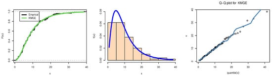
Figure 5. Estimated PDF and CDF with lines plots and Q-Q plot: data I.

For data II: From Table 12, the MLEs (with their SE) of $\theta$ and $\lambda$, meanwhile the KS (p-value) was 0.1198 (0.8579). It means that the KMGE lifetime model fits the number of hours (in thousands) between failures of secondary reactor pumps data well. Figure 6 illustrates the estimated and empirical CDF of KMGE on the left, the estimated and histogram of KMGE density in the center, and the Q-Q of KMGE on the right for the number of hours (in thousands) between the failures of the secondary reactor pump data using a graphic visualization. From the results in Table 12, we can confirm that data II fitted the KMGE distribution.

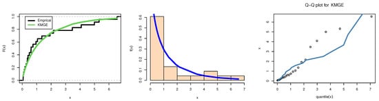
Figure 6. Estimated PDF and CDF with lines plots and Q-Q plot: data II.

For the GTI-PHCS of data I: Different GTI-PHCS samples (where m = 80, $\mathcal{K}$ = 70, and $\tau$ = 12) based on various CS selections were obtained from the waiting period before getting the banking service data and are shown in Table 13 to evaluate our acquired estimators. Also, MLE and Bayesian estimates based on GTI-PHCS for data I have been obtained in Table 14.

Table 13. Sample observation based on GTI-PHCS: data I.

CS	Observation	$\overline{\mathcal{K}}$
1	0.8 0.8 1.3 1.5 1.8 1.9 1.9 2.1 2.6 2.7 2.9 3.1 3.2 3.3 4.1 4.2 4.3 4.4 4.4 4.6 4.7 4.7 4.8 4.9 4.9 5.5 5.7 5.7 6.1 6.2 6.2 6.3 6.7 6.9 7.1 7.1 7.1 7.1 7.6 7.7 8.2 8.6 8.6 8.8 8.8 9.5 9.6 9.7 10.7 10.9 11.0 11.1 11.2 11.2 11.5	55
2	0.8 0.8 1.3 1.5 1.8 1.9 1.9 2.6 2.9 3.1 3.2 3.3 3.6 4.0 4.1 4.2 4.2 4.3 4.3 4.4 4.4 4.6 4.8 4.9 4.9 5.0 5.5 5.7 5.7 6.1 6.2 6.2 6.3 6.7 6.9 7.1 7.1 7.4 7.6 7.7 8.0 8.6 8.6 8.8 8.8 8.9 9.5 9.6 9.7 9.8 10.7 10.9 11.0 11.0 11.1 11.2 11.9	57
3	0.8 0.8 1.3 1.5 1.8 1.9 1.9 2.1 2.6 2.7 2.9 3.1 3.2 3.3 3.5 3.6 4.0 4.1 4.2 4.2 4.3 4.3 4.4 4.4 4.6 4.7 4.7 4.8 4.9 4.9 5.0 5.3 5.5 5.7 5.7 6.1 6.2 6.2 6.2 6.3 6.7 6.9 7.1 7.1 7.1 7.1 7.4 7.6 7.7 8.0 8.2 8.6 8.6 8.6 8.8 8.8 8.9 8.9 9.5 9.6 9.7 9.8 10.7 10.9 11.0 11.0 11.1 11.2 11.2 11.5 11.9	71
4	0.8 0.8 1.3 1.5 1.8 1.9 1.9 2.1 2.6 2.7 2.9 3.1 3.2 3.3 3.6 4.0 4.1 4.2 4.2 4.3 4.3 4.4 4.4 4.6 4.7 4.8 4.9 4.9 5.0 5.5 5.7 5.7 6.1 6.2 6.2 6.2 6.3 6.7 6.9 7.1 7.1 7.4 7.6 7.7 8.0 8.6 8.6 8.8 8.8 8.9 8.9 9.5 9.6 9.7 9.8 10.7 10.9 11.0 11.0 11.1 11.2 11.5 11.9	63

Table 14. MLE and Bayesian Estimate based on GTI-PHCS: data I.

		MLE		Bayesian
CS		Estimates	SE	Bayes	SEBayes
1	$\theta$	2.1173	0.3615	2.3120	0.3444
	$\lambda$	0.1213	0.0210	0.1322	0.0191
2	$\theta$	2.2197	0.3847	2.3149	0.3347
	$\lambda$	0.1312	0.0218	0.1366	0.0184
3	$\theta$	2.2943	0.3722	2.3563	0.3424
	$\lambda$	0.1331	0.0199	0.1366	0.0181
4	$\theta$	2.1549	0.3594	2.2909	0.3154
	$\lambda$	0.1261	0.0203	0.1345	0.0181

For the GTI-PHCS of data II: Different GTI-PHCS samples (where m = 20, $\mathcal{K}$ = 15, and $\tau$ = 2) based on various CS as

CS.1: $R_1=2$, $R_2=1$ and the $R_i=0$ where $i=3,\dots ,m$.

CS.2: $R_1=3$, and the $R_i=0$ where $i=2,\dots ,m$.

CS.3: $R_m=3$, and the $R_i=0$ where $i=1,\dots ,m-1$.

CS.4: $R_1=2$, $R_2=1$ and the $R_i=0$ where $i=2,\dots ,m-1$.

selections were obtained from the number of hours (in thousands) between failures of secondary reactor pumps data and are shown in Table 15 to evaluate our acquired estimators.

Table 15. Sample observation based on GTI-PHCS: data II.

CS	Observation	$\overline{\mathcal{K}}$
1	0.062 0.070 0.101 0.150 0.199 0.273 0.347 0.358 0.402 0.491 0.605 0.614 0.746 0.954 1.060	15
2	0.062 0.070 0.101 0.150 0.199 0.273 0.347 0.358 0.402 0.491 0.605 0.614 0.746 0.954 1.921	15
3	0.062 0.070 0.101 0.150 0.199 0.273 0.347 0.358 0.402 0.491 0.605 0.614 0.746 0.954 1.060 1.359 1.921	17
4	0.062 0.070 0.101 0.150 0.199 0.273 0.347 0.358 0.402 0.491 0.491 0.605 0.614 0.746 0.954 1.060 1.921	16

Figure 7 and Figure 8 discussed the contour of the log-likelihood function in relation to different $\theta$ and $\lambda$ values. It confirmed the results of the KS test and demonstrated the existence, uniqueness, and originality of the MLE. The Bayes estimates (along with their SE) were assessed using gamma priors which are also supplied in Table 14 and Table 16 because there was no prior knowledge about the unknown KMGE parameters $\theta$ and $\lambda$ from the available data set. Figure 9 and Figure 10 show the trace plots of each generated sample to show how the MCMC iterations have converged. Figure 11 and Figure 12 discussed MCMC posterior density and scatter plot for parameters based on CS.4 for data I, data II, respectively.

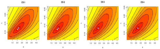
Figure 7. Contour plots: data I.

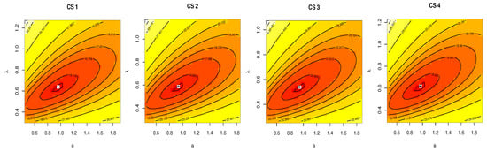
Figure 8. Contour plots: data II.

Table 16. MLE and Bayesian Estimate based on GTI-PHCS: data II.

		MLE		Bayesian
CS		Estimates	SE	Bayes	SEBayes
1	$\theta$	0.9451	0.2726	0.9307	0.2508
	$\lambda$	0.6276	0.2843	0.6267	0.2656
2	$\theta$	0.9151	0.2605	0.8824	0.2362
	$\lambda$	0.5770	0.2640	0.5357	0.2342
3	$\theta$	0.9283	0.2576	0.9225	0.2466
	$\lambda$	0.5299	0.2265	0.5372	0.2047
4	$\theta$	0.9514	0.2679	0.9306	0.2599
	$\lambda$	0.6075	0.2623	0.5903	0.2378

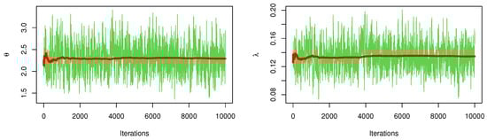
Figure 9. MCMC trace plot with convergence line: data I, CS.4.

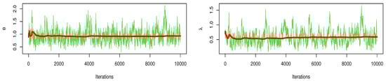
Figure 10. MCMC trace with convergence line: data II, CS.4.

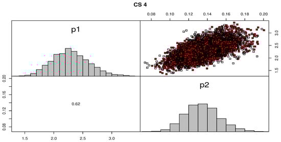
Figure 11. MCMC posterior density and scatter plot: data I, CS.4.

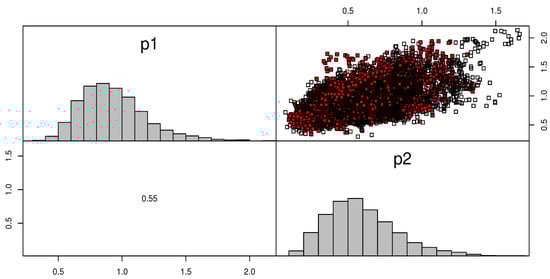
Figure 12. MCMC posterior density and scatter plot: data II, CS.4.

7. Concluding Remarks

In this paper, we considered the problems of parameter estimation of the KMGE distribution under the generalized progressively hybrid censored samples. For point estimation, five classical approaches of estimation such as ML, MPS, LS, WLS, and PE are discussed. Moreover, the Bayesian approach is studied. For interval estimation, we use the ML method of estimation by using the normal approximation confidence interval and the normal approximation of log-transformed MLE. The considered five classical estimation methods were then compared in terms of RB, MSEr, ARB, AMSEr, and AL of CI via Monte Carlo simulations. The MPS method shows better performance than the other four classical estimation methods for most of the considered cases. Bayesian estimation of the unknown parameters is presented under informative prior using two different loss functions. The results in the illustrative example show that the proposed ML and Bayesian work well again. In summary, the improved estimation methods of the ML, MPS, LS, WLS, PE, and Bayesian approaches contribute to more accurate parameter estimation for the KMGE distribution. These methods have practical utility in industries such as finance, insurance, engineering, healthcare, environmental modeling, social sciences, and more. By utilizing these estimation methods, practitioners can obtain reliable parameter estimates, leading to improved decision-making and predictive modeling in real-world applications. Future studies will take into account the estimation problem based on a broad framework called unified hybrid censoring.

References

- Epstein, B. Truncated life-tests in the exponential case. Ann. Math. Statist. 1954, 25, 555–564. [Google Scholar] [CrossRef]
- Cohen, A.C. Progressively censored samples in life testing. Technometrics 1963, 5, 327–329. [Google Scholar] [CrossRef]
- Kundu, D.; Joarder, A. Analysis of type-II progressively hybrid censored data. Comput. Statist. Data Anal. 2006, 50, 2509–2528. [Google Scholar] [CrossRef]
- Cho, Y.; Sun, H.; Lee, K. Exact likelihood inference for an exponential parameter under generalized progressive hybrid CS. Statist. Method. 2015, 23, 18–34. [Google Scholar] [CrossRef]
- El-Sherpieny, E.S.A.; Almetwally, E.M.; Muhammed, H.Z. Progressive Type-II hybrid censored schemes based on maximum product spacing with application to Power Lomax distribution. Phys. A Stat. Mech. Its Appl. 2020, 553, 124251. [Google Scholar] [CrossRef]
- Cho, Y.; Sun, H.; Lee, K. Estimating the entropy of a Weibull distribution under generalized progressive hybrid censoring. Entropy 2015, 17, 102–122. [Google Scholar] [CrossRef]
- Salem, S.; Abo-Kasem, O.E.; Hussien, A. On Joint Type-II Generalized Progressive Hybrid Censoring Scheme. Comput. J. Math. Stat. Sci. 2023, 2, 123–158. [Google Scholar] [CrossRef]
- Zhang, C.; Shi, Y. Statistical prediction of failure times under generalized progressive hybrid censoring in a simple step-stress accelerated competing risks model. J. Syst. Eng. Elect. 2017, 28, 282–291. [Google Scholar]
- Wang, L.; Tripathi, Y.M.; Lodhi, C. Inference for Weibull competing risks model with partially observed failure causes under generalized progressive hybrid censoring. J. Comput. Appl. Math. 2020, 368, 112537. [Google Scholar] [CrossRef]
- Koley, A.; Kundu, D. On generalized progressive hybrid censoring in presence of competing risks. Metrika 2017, 80, 401–426. [Google Scholar] [CrossRef]
- Abdel-Hamid, A.H.; Hashem, A.F. Inference for the Exponential Distribution under Generalized Progressively Hybrid Censored Data from Partially Accelerated Life Tests with a Time Transformation Function. Mathematics 2021, 9, 1510. [Google Scholar] [CrossRef]
- Sayed-Ahmed, N.; Jawa, T.M.; Aloafi, T.A.; Bayones, F.S.; Elhag, A.A.; Bouslimi, J.; Abd-Elmougod, G.A. Generalized Type-I hybrid censoring scheme in estimation competing risks Chen lifetime populations. Math. Probl. Eng. 2021, 2021, 6693243. [Google Scholar] [CrossRef]
- Nagy, M.; Alrasheedi, A.F. The lifetime analysis of the Weibull model based on Generalized Type-I progressive hybrid censoring schemes. Math. Biosci. Eng. 2022, 19, 2330–2354. [Google Scholar] [CrossRef] [PubMed]
- Nagy, M.; Alrasheedi, A.F. Estimations of generalized exponential distribution parameters based on Type I generalized progressive hybrid censored data. Comput. Math. Methods Med. 2022, 2022, 8058473. [Google Scholar] [CrossRef] [PubMed]
- Gupta, R.C.; Gupta, P.L.; Gupta, R.D. Modeling failure time data by Lehman alternatives. Commun. Stat.-Theory Methods 1998, 27, 887–904. [Google Scholar] [CrossRef]
- Mudholkar, G.S.; Srivastava, D.K. Exponentiated Weibull family for analyzing bathtub failure-rate data. IEEE Trans. Reliab. 1993, 42, 299–302. [Google Scholar] [CrossRef]
- Mudholkar, G.S.; Srivastava, D.K.; Freimer, M. The exponentiated Weibull family: A reanalysis of the bus-motor-failure data. Technometrics 1995, 37, 436–445. [Google Scholar] [CrossRef]
- Barreto-Souza, W.; Santos, A.H.; Cordeiro, G.M. The beta generalized exponential distribution. J. Stat. Comput. Simul. 2010, 80, 159–172. [Google Scholar] [CrossRef]
- Ristic, M.M.; Kundu, D. Marshall-Olkin generalized exponential distribution. Metron 2015, 73, 317–333. [Google Scholar] [CrossRef]
- Chaudhary, A.K.; Sapkota, L.P.; Kumar, V. Half-Cauchy Generalized Exponential Distribution: Theory and Application. J. Nepal Math. Soc. (JNMS) 2022, 5, 1–10. [Google Scholar] [CrossRef]
- Sapkota, L.P.; Kumar, V. Odd Lomax Generalized Exponential Distribution: Application to Engineering and COVID-19 data. Pak. J. Stat. Oper. Res. 2022, 18, 883–900. [Google Scholar] [CrossRef]
- Astorga, J.M.; Iriarte, Y.A.; Gómez, H.W.; Bolfarine, H. Modified slashed generalized exponential distribution. Commun. Stat.-Theory Methods 2019, 49, 4603–4617. [Google Scholar] [CrossRef]
- Alotaibi, N.; Elbatal, I.; Almetwally, E.M.; Alyami, S.A.; Al-Moisheer, A.S.; Elgarhy, M. Bivariate Step-Stress Accelerated Life Tests for the Kavya-Manoharan Exponentiated Weibull Model under Progressive Censoring with Applications. Symmetry 2022, 14, 1791. [Google Scholar] [CrossRef]
- Meeker, W.Q.; Escobar, L.A. Statistical Method for Reliability Data; Wiley: New York, NY, USA, 1998. [Google Scholar]
- Cheng, R.C.H.; Amin, N.A.K. Estimating parameters in continuous univariate distributions with a shifted origin. J. R. Stat. Soc. B 1983, 45, 394–403. [Google Scholar] [CrossRef]
- Ng, H.K.T.; Luo, L.; Hu, Y.; Duan, F. Parameter estimation of three-parameter Weibull distribution based on progressively type-II censored samples. J. Stat. Comput. Simul. 2012, 82, 1661–1678. [Google Scholar] [CrossRef]
- Alotaibi, N.; Hashem, A.F.; Elbatal, I.; Alyami, S.A.; Al-Moisheer, A.S.; Elgarhy, M. Inference for a Kavya–Manoharan Inverse Length Biased Exponential Distribution under Progressive-Stress Model Based on Progressive Type-II Censoring. Entropy 2022, 24, 1033. [Google Scholar] [CrossRef] [PubMed]
- Swain, J.J.; Venkatraman, S.; Wilson, J.R. Least-squares estimation of distribution function in Johnson’s translation system. J. Statist. Comput. Simul. 1988, 29, 271–297. [Google Scholar] [CrossRef]
- Abdel-Hamid, A.H.; Hashem, A.F. A new lifetime distribution for a series-parallel system: Properties, applications and estimations under progressive type-II censoring. J. Statist. Comput. Simul. 2017, 87, 993–1024. [Google Scholar] [CrossRef]
- Hashem, A.F.; Alyami, S.A. Inference on a New Lifetime Distribution under Progressive Type-II Censoring for a Parallel-Series structure. Complexity 2021, 2021, 6684918. [Google Scholar] [CrossRef]
- Hashem, A.F.; Kuş, C.; Pekgör, A.; Abdel-Hamid, A.H. Poisson-logarithmic half-logistic distribution with inference under a progressive-stress model based on adaptive type-II progressive hybrid censoring. J. Egypt Math. Soc. 2022, 30, 15. [Google Scholar] [CrossRef]
- Aggarwala, R.; Balakrishnan, N. Some properties of progressive censored order statistics from arbitrary and uniform distributions with applications to inference and simulation. J. Stat. Plann. Inf. 1998, 70, 35–49. [Google Scholar] [CrossRef]
- Kao, J.H.K. A graphical estimation of mixed Weibull parameters in life testing electron tube. Technometrics 1959, 1, 389–407. [Google Scholar] [CrossRef]
- Dey, S.; Ali, S.; Park, C. Weighted exponential distribution: Properties and different methods of estimation. J. Stat. Comput. Simul. 2015, 85, 3641–3661. [Google Scholar] [CrossRef]
- Dey, S.; Singh, S.; Tripathi, Y.M.; Asgharzadeh, A. Estimation and prediction for a progressively censored generalized inverted exponential distribution. Stat. Methodol. 2016, 32, 185–202. [Google Scholar] [CrossRef]
- Hamdy, A.; Almetwally, E.M. Bayesian and Non-Bayesian Inference for The Generalized Power Akshaya Distribution with Application in Medical. Comput. J. Math. Stat. Sci. 2023, 2, 31–51. [Google Scholar] [CrossRef]
- Varian, H.R. Bayesian approach to real estate assessment. In Studies in Bayesian Econometrics and Statistics; Savage, L.J., Feinderg, S.E., Zellner, A., Eds.; North-Holland: Amsterdam, The Netherlands, 1975; pp. 195–208. [Google Scholar]
- Bantan, R.; Hassan, A.S.; Almetwally, E.; Elgarhy, M.; Jamal, F.; Chesneau, C.; Elsehetry, M. Bayesian analysis in partially accelerated life tests for weighted lomax distribution. Comput. Mater. Contin 2021, 68, 2859–2875. [Google Scholar] [CrossRef]
- Almongy, H.M.; Almetwally, E.M.; Alharbi, R.; Alnagar, D.; Hafez, E.H.; Mohie El-Din, M.M. The Weibull generalized exponential distribution with censored sample: Estimation and application on real data. Complexity 2021, 2021, 6653534. [Google Scholar] [CrossRef]
- Alotaibi, R.; Alamri, F.S.; Almetwally, E.M.; Wang, M.; Rezk, H. Classical and Bayesian Inference of a Progressive-Stress Model for the Nadarajah–Haghighi Distribution with Type II Progressive Censoring and Different Loss Functions. Mathematics 2022, 10, 1602. [Google Scholar] [CrossRef]
- Henningsen, A.; Toomet, O. maxLik: A package for maximum likelihood estimation in R. Comput. Stat. 2011, 26, 443–458. [Google Scholar] [CrossRef]
- Ghitany, M.E.; Atieh, B.; Nadarajah, S. Lindley distribution and its application. Math. Comput. Simul. 2008, 78, 493–506. [Google Scholar] [CrossRef]
- Suprawhardana, M.S.; Prayoto, S. Total time on test plot analysis for mechanical components of the RSG-GAS reactor. At. Indones 1999, 25, 81–90. [Google Scholar]
Disclaimer/Publisher’s Note: The statements, opinions and data contained in all publications are solely those of the individual author(s) and contributor(s) and not of MDPI and/or the editor(s). MDPI and/or the editor(s) disclaim responsibility for any injury to people or property resulting from any ideas, methods, instructions or products referred to in the content. |
© 2023 by the authors. Licensee MDPI, Basel, Switzerland. This article is an open access article distributed under the terms and conditions of the Creative Commons Attribution (CC BY) license (https://creativecommons.org/licenses/by/4.0/).