Two-Dimensional Moran Model

Abstract

In this paper, we consider a two-dimensional Moran model of random walks consisting of two queues evolving in parallel which can (at each unit of time) either increase by one or reset to 0. We analyze the joint law of their final altitude and prove that the asymptotic distribution of each component is a shifted geometric distribution and we analyze the maximum of these two components, also giving closed forms for the mean and variance.

1. Introduction

The concept of a random walk is very important and is used in many fields, such as in biology (random walk is applied to problems related to genetic diseases such as diabetes, cancer, or the movement of an animal in search of food), physics (the movement of a particle in a gas or liquid), chemistry, (a chemical reagent in a solution), economics (the stock market price), the maximum age of a machine in mechanics, the exploration of a territory by a robot in artificial intelligence, etc.

In this article, we consider discrete random walks. Many scientific studies used probability generating functions to obtain the mean, the variance, and the limiting distribution of some statistics such as the final altitude and the height of discrete random walks, e.g., via the kernel method and singularity analysis (see [1,2]), via some links with continued fractions [3], or via more probabilistic approaches (see [4], which also illustrates links with random trees).

For example in dimension one, if one focuses on articles which play a role in our analysis, Banderier and Flajolet have shown in [1] that the final altitude of a random meander of length n converges asymptotically to a Rayleigh distribution (drift $\delta =0$) and normal distribution ($\delta >0$). Furthermore, in [5], Banderier and Nicodème have analyzed the height of discrete bridges/meanders/excursions for bounded discrete walks. Similar extremal parameters were also studied for trees in [4,6], and by Gafni [7] for the asymptotic distribution of the length of the longest run of consecutive equal parts. Finally, some models of walks with reset were considered by Banderier and Wallner, who treated some statistics for lattice paths with catastrophes such as the number of catastrophes of a random excursion of size n, which converges to Gaussian, Rayleigh, or discrete distribution depending on the drift (see Theorem 4.12 in [8]).

Then for higher dimensions, still in link with our model, we can mention the stochastic model for solitons, investigated by Itoh, Mahmoud, and Takahashi in [9], where they proved that the wavelength converges to a convolution of geometric random variables. Itoh and Mahmoud [10] also proved that the distribution for the lifetime of an individual converges to a (shifted) geometric distribution in law. Other articles related to the Moran process (in biology and population genetics) are involving similar higher-dimensional walk models; see e.g., [11,12,13].

In this paper, we study the two-dimensional Moran walk TDMW defined as follows: At time 0, the process starts from the origin. After one unit of time, we have four possibilities: (a) the process stops at (0,0) with probability $p_0$; (b) the first component shifts by one positive unit, but the second component returns to zero with probability $p_1$; (c) the second component shifts by one positive unit, but the first component returns to zero with probability $p_2$; or (d) the two components shift by one positive unit with probability p. We now provide four examples of the evolution of the TDMW process until time $n=8$:

$$(0,0)\stackrel{p_1}{\to }(0,1)\stackrel{p}{\to }(1,2)\stackrel{p_1}{\to }(0,3)\stackrel{p_2}{\to }(1,0)\stackrel{p_2}{\to }(2,0)\stackrel{p}{\to }(3,1)\stackrel{p}{\to }(4,2)\stackrel{p_1}{\to }(0,3)$$

(1)

$$(0,0)\stackrel{p_0}{\to }(0,0)\stackrel{p}{\to }(1,1)\stackrel{p_1}{\to }(0,1)\stackrel{p_2}{\to }(1,0)\stackrel{p_2}{\to }(2,0)\stackrel{p}{\to }(3,1)\stackrel{p_2}{\to }(4,0)\stackrel{p}{\to }(5,1)$$

(2)

$$(0,0)\stackrel{p}{\to }(1,1)\stackrel{p}{\to }(2,2)\stackrel{p}{\to }(3,3)\stackrel{p_2}{\to }(4,0)\stackrel{p_2}{\to }(5,0)\stackrel{p}{\to }(6,1)\stackrel{p_2}{\to }(7,0)\stackrel{p_2}{\to }(8,0)$$

(3)

$$(0,0)\stackrel{p_2}{\to }(1,0)\stackrel{p}{\to }(2,1)\stackrel{p_1}{\to }(0,2)\stackrel{p_1}{\to }(0,3)\stackrel{p_1}{\to }(0,4)\stackrel{p}{\to }(1,5)\stackrel{p}{\to }(2,6)\stackrel{p}{\to }(3,7).$$

(4)

In these four examples, the final altitude of components one and two are 0, 5, 8, 3, and 3, 1, 0, 7, respectively. The final altitude of the maximum is 3, 5, 8, and 7 and the height of the four walks is 4, 5, 8, and 7, respectively.

The main result of this work is the discovery of the probability generating function of the maximum of the two final altitudes, and the computation of the corresponding mean and variance. Furthermore, we prove that the asymptotic distribution of the two random walks converges to a shifted geometric distribution, and we give a closed form for the corresponding mean and variance.

This paper is organized as follows. In Section 2, we define some statistics, introduce our model in detail, and use some examples for different lengths of Moran walk according to the probability distribution. In Section 3, we state our main results on the probability generating function of the final altitude and their mean and variance. In Section 4, we use R software to simulate Moran walks of lengths: 10, 100, 500, and 1000, for different values of the probabilities $p_0$, $p_1$, $p_2$, and p. In Section 5, we establish recursive equations for the sequence of multivariate polynomials and the probability generating function associated with the model. In Section 6, we prove that the limiting distributions of two Moran random walks $Y_n^{\left(1\right)}$ and $Y_n^{\left(2\right)}$ converge to shifted geometric distributions and find their means and variances. In Section 7, we give the proofs of our theorems. In Section 8, we present another method for obtaining the distribution of the final altitude $Y_n$. Finally, we present some conclusions and perspectives.

2. Definitions and Presentation of the Model

In this section, we present some definitions concerning the statistical properties of discrete processes, such as the mean, the variance, and the probability generating function. Finally, we present our model and define some statistics, such as the final altitude and height.

Let us consider a stochastic process with a discrete time and finite state space without assuming that they are Markov chains. For brevity, we call such a process a discrete stochastic process. We start with the following classical definitions (see [14]).

2.1. Definitions

1.

Let $U=(U_n,n=0,1,2,\cdots )$ be a discrete stochastic process starting from time $n=0$, with $U_0$ being the initial state.

2.

The state space of the process is assumed to be finite and is denoted by S. Each $U_n$ takes its values in S.

3.

Let $(U,V)=((U_n,V_n),n=0,1,2,\cdots )$ be a discrete stochastic process with two dimensions starting from time $n=0$, with $(U_0,V_0)=(0,0)$ being the initial state.

4.

The state space of the process is assumed to be finite and is denoted by $S\times S$. Each $(U_n,V_n)$ takes their values in $S\times S$.

5.

The probability distribution of $U_n$ is denoted by $P_n$, which is identified with a vector in ${[0,1]}^S$. We call these distributions the one-dimensional distributions of the process.

6.

We define the probability that is associated with the discrete process $(U_n,V_n)$ as follows: for all $r,s\in \mathbb{N}$, $P_n(r,s)=P(U_n=r,V_n=s).$

7.

Let U be a discrete random variable with a distribution $P(U=r)=p_r$, $r\in \mathbb{N}$. Then, the expected value and variance of U, denoted by $\mathbb{E}\left(U\right)$ and $\mathbb{V}\mathrm{ar}\left(U\right)$, respectively, is defined as

$${\displaystyle \mathbb{E}\left(U\right)=\sum _{r\ge 0}r{p}_{r}and\mathbb{V}\mathrm{ar}\left(U\right)=\mathbb{E}\left({\left[U-\mathbb{E}\left(U\right)\right]}^2\right)=\mathbb{E}\left(U^2\right)-{\left(\mathbb{E}\left(U\right)\right)}^2.}$$

8.

Let U be a discrete random variable with distribution $P(U=r)=p_r$, $r\in \mathbb{N}$; then, the probability generating function, denoted by G, of the variable U is defined by:

$${\displaystyle G_U\left(u\right)=\mathbb{E}\left(u^U\right)=\sum _{r=0}^{\infty }{u}^r{p}_r,}$$

for all $u\in \mathbb{R}$ such that $\left|u\right|<1$.

Probability generating functions constitute an elegant tool due to their numerous uses. Mainly, the probability density functions associated with discrete stochastic processes and their moments can be obtained from the derivatives of the probability generating function. In fact, the mean and the variance of the process (the first and second centered moments of the distribution of U) are related to the derivatives of the probability generating function at $u=1$. More precisely, the next folklore lemma explains this link.

Lemma 1 

([2]). Let $G_U$ be the probability generating function for the discrete random process random U; then, for $k\in \mathbb{N}$, the kth factorial moment of U is given by

$$\frac{{\partial }^k{G}_U\left(u\right)}{{\partial }^{k}u}{|}_{u=1}=\mathbb{E}\left(U(U-1)(U-2)\dots (U-k+1)\right).$$

In addition, if the limit of $\frac{\partial G_U\left(u\right)}{\partial u}$ and $\frac{{\partial }^2{G}_U\left(u\right)}{{\partial }^{2}u}$ exists at $u=1$, then we have the following two important equations, which are related to the mean and variance of U and $G_U\left(u\right)$:

$$\mathbb{E}\left(U\right)=\frac{\partial G_U\left(u\right)}{\partial u}{|}_{u=1}\mathrm{and}\mathbb{V}\mathrm{ar}\left(U\right)=\frac{{\partial }^2{G}_U\left(u\right)}{{\partial }^{2}u}{|}_{u=1}+\mathbb{E}\left(U\right)-\mathbb{E}{\left(U\right)}^2.$$

(5)

Consider a two-dimensional Moran model with two components $Y_n^{\left(1\right)},Y_n^{\left(2\right)}$; it starts at time 0 with two components having an age 0 (i.e., $(Y_0^{\left(1\right)},Y_0^{\left(2\right)})=(0,0)$), and it is parameterized by four probabilities, denoted by $p_0$, $p_1$, $p_2$, and p. The Moran model with two dimensions is given by the following system:

$$\begin{array}{cc}\hfill (Y_{n+1}^{\left(1\right)},Y_{n+1}^{\left(2\right)})& =\left\{\begin{array}{cc}(Y_n^{\left(1\right)}+1,Y_n^{\left(2\right)}+1),\hfill & \mathrm{with}\mathrm{probability}p,\hfill \\ \\ (0,Y_n^{\left(2\right)}+1),\hfill & \mathrm{with}\mathrm{probability}{p}_1,\hfill \\ \\ (Y_n^{\left(1\right)}+1,0),\hfill & \mathrm{with}\mathrm{probability}{p}_2,\hfill \\ \\ (0,0),\hfill & \mathrm{with}\mathrm{probability}{p}_0,\hfill \end{array}\right.\hfill \end{array}$$

(6)

where $p_0,p_1,p_2,$ and p are non-negative given values such that $p+p_0+p_1+p_2=1$.

Additionally, we define the final altitude $Y_n$ and height $H_n$ statistics by:

$$\begin{array}{cc}\hfill Y_n& =max(Y_n^{\left(1\right)},Y_n^{\left(2\right)}),\hfill \\ \hfill H_n& =max(Y_0,Y_1,Y_2,\cdots ,Y_n).\hfill \end{array}$$

Applying the four first definitions, we can consider $Y_n$ and $H_n$ as a random walk (discrete stochastic process with one dimension) in the state space $S=\{0,\dots ,n\}$, which is started from the initial state $Y_0=0$ and $H_0=0$, respectively. However, $(Y_n^{\left(1\right)},Y_n^{\left(2\right)})$ are considered a stochastic process with two dimensions in the state space $S^2={\{0,\dots ,n\}}^2$, which is started from the initial state $(Y_0^{\left(1\right)},$$Y_0^{\left(2\right)})=(0,0)$. Moreover, we can consider $Y_n^{\left(1\right)}$, $Y_n^{\left(2\right)}$, $Y_n$, and $H_n$ as a random walk in ${\mathbb{N}}^2$, where the x-axis represents the time n (length of Moran walk) and the y-axis represents the age of each component $Y_n^{\left(1\right)}$ and $Y_n^{\left(2\right)}$ or the maximum age or the height. In the next section, we denote by:

$\mathbb{E}\left(Y_n^{\left(i\right)}\right)$, $\mathbb{V}\mathrm{ar}\left(Y_n^{\left(i\right)}\right)$, and $\mathbb{E}\left(Y_n\right)$ for the means and variances of $Y_n^{\left(i\right)}$ and $Y_n$ for $i=1,2$ and $n\ge 0$, respectively.

2.2. Example 1: Two-Dimensional Moran Walk of Length 5 for Initial Probabilities $p_0=p=1/6$ and $p_1=p_2=1/3$

Using R software, Figure 1 shows that the final altitudes of the two components are equal to two and one, respectively; thus, the final maximum age of the two components is equal to two. In addition, the age height is fixed at two when $p_0=p=1/6$ and $p_1=p_2=1/3$ for the Moran walk of length 5.

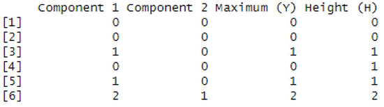
Figure 1. The evolution of the age of each component, the final altitude, and the height of two-dimensional Moran walk of length 5 starting from $(0,0)$.

2.3. Example 2: Two-Dimensional Moran Walk of Length 10 with Initial Probabilities $p_0=p=1/6$ and $p_1=p_2=1/3$

Figure 2 shows that the final altitudes of the two components are equal to one and two, respectively; thus, the final maximum age of the two components is equal to two. In addition, the age height is 4 at time 7, when $p_0=p=1/6$ and $p_1=p_2=1/3$ for the Moran walk of length 10.

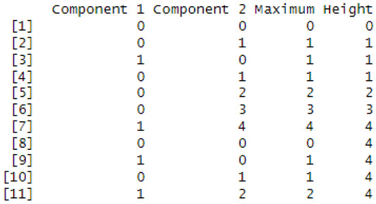
Figure 2. The evolution of the age of each component, the final altitude, and the height of the two-dimensional Moran walk of length 10 starting from $(0,0)$.

3. Main Result

In this section, we study the final altitude of the maximum age, $Y_n=max(Y_n^1,Y_n^2)$, between the two components at time n. Precisely, we want to find the probability generating function of $Y_n$, denoted by ${\Psi }_n\left(x\right)$, and determine the mean and variance of the Moran walk $Y_n$ with length n. For this reason, we define the probability generating function ${\Psi }_n\left(x\right)$ as

$${\displaystyle \forall x\in \mathbb{R},{\Psi }_n\left(x\right)=G_{Y_n}\left(x\right)=\sum _{k=0}^n{x}^{k}P(Y_n=k)=\sum _{k=0}^n{x}^{k}P\left(max(Y_n^{\left(1\right)},Y_n^{\left(2\right)})=k\right).}$$

(7)

The first result concerns the probability generating function ${\Psi }_n\left(x\right)$, which is presented in the next theorem.

Theorem 1. 

The probability generating function, ${\Psi }_n\left(x\right)$, of the final altitude between the two components $Y_n=max(Y_n^{\left(1\right)},Y_n^{\left(2\right)})$ is given by the following: for all $n\in {\mathbb{N}}^{*}$, $x\in \mathbb{R}$,

$$\begin{array}{ccc}\hfill {\displaystyle {\Psi }_n\left(x\right)}& =& {\displaystyle 2p_0-\left(p_1+p_2\right)\frac{px-{\left(px\right)}^n}{1-px}+\left(r_1^n+r_2^n\right)x^n+(1-r_1)\frac{r_{1}x-{\left(r_{1}x\right)}^n}{1-r_{1}x}}\hfill \\ & & {\displaystyle +(1-r_2)\frac{r_{2}x-{\left(r_{2}x\right)}^n}{1-r_{2}x}-p_0\frac{1-{\left(px\right)}^n}{1-px}-{\left(px\right)}^n,}\hfill \end{array}$$

such that ${\displaystyle {\Psi }_0\left(x\right)=1}$, where $r_1=p_2+p$, $r_2=p_1+p$, $|r_1{x}_1|<1$, $|r_2{x}_2|<1$ and $\left|px\right|<1$.

In the next theorem, using the probability generating function and their derivatives of order one and two, respectively, we can calculate the mean and variance of $Y_n$. The second main result is presented in the following theorem.

Theorem 2. 

The mean and variance of the final altitude $Y_n$ are given by

$$\begin{array}{c}\hfill {\displaystyle \mathbb{E}\left(Y_n\right)=\frac{r_1-r_1^{n+1}}{1-r_1}+\frac{r_2-r_2^{n+1}}{1-r_2}-\frac{p-p^{n+1}}{1-p},}\end{array}$$

(8)

and

$$\begin{array}{cc}\hfill \mathbb{V}\mathrm{ar}\left(Y_n\right)=& \frac{r_1}{{(1-r_1)}^2}\left(1-r_1^n\left\{r_1^{n+1}+(1+2n)(1-r_1)\right\}\right)\hfill \\ \hfill & +\frac{r_2}{{(1-r_2)}^2}\left(1-r_2^n\left\{r_2^{n+1}+(1+2n)(1-r_2)\right\}\right)\hfill \\ \hfill & -\frac{p}{{(1-p)}^2}\left(3p+p^n\left\{p^{n+1}-2n(1-p)-4p\right\}\right)\hfill \\ \hfill & +2\left(\frac{r_1-r_1^{n+1}}{1-r_1}+\frac{r_2-r_2^{n+1}}{1-r_2}\right)\left(\frac{p-p^{n+1}}{1-p}\right)\hfill \\ \hfill & -2\left(\frac{r_1-r_1^{n+1}}{1-r_1}\right)(\frac{r_2-r_2^{n+1}}{1-r_2}),\hfill \end{array}$$

where $r_1=p_2+p$ and $r_2=p_1+p$.

Remark 1. 

Because $Y_n=max(Y_n^{\left(1\right)},Y_2^{\left(2\right)})$, then $Y_n\ge Y_n^{\left(i\right)}$, for $i=1,2$. So, we deduce from Theorem 2 and Corollary 1 that $\mathbb{E}\left(Y_n\right)\ge \mathbb{E}\left(Y_n^{\left(i\right)}\right)$.

4. Simulation

In this section, using R software, we simulate the final altitude of each component $Y^{\left(1\right)}$, $Y^{\left(2\right)}$, the maximum Y, and the height H for two cases. In the first case, we take $p_0=p=1/6$ and $p_1=p_2=1/3$ in the system (6); in the second case, we take $p_0=p=1/8$ and $p_1=p_2=3/8$ for four different lengths of the TDMW, which are equal to 10, 100, 500, and 1000, respectively.

Figure 3 shows that the final altitudes of $Y^{\left(1\right)}$, $Y^{\left(2\right)}$, Y, and H are equal to 0, 2, 2, and 3 for the Moran walk of length 10. When the length is increased from 10 to 100, we observe that the final altitudes $Y^{\left(1\right)}$, $Y^{\left(2\right)}$, Y, and H are equal to 2, 0, 2, and 8. It is clear that the height is bounded by eight. Then the maximum age of the two components over the full process goes from 6 (for length 10) to 8 (for length 100). This increase is very small, this can be explained by a logarithmic increase of the height over the time, similarly to what is proven in [15].

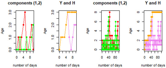
Figure 3. Final altitude of $Y^{\left(1\right)}$ (in red), $Y^{\left(2\right)}$ (in green), their maximum ($Y:=max(Y^{\left(1\right)},Y^{\left(2\right)})$, in pick) and height H (in orange) of a TDMW of lengths 10 and 100 for $p_0=p=1/8$ and $p_1=p_2=3/8$.

Figure 4 shows that if the length is equal to 500, the final altitudes of $Y^{\left(1\right)}$, $Y^{\left(2\right)}$, and Y are equal to at most 4, and the final altitude of the height H is equal to 10. If we increase the length of the walk from 500 to 1000, then we remark that the final altitudes of $Y^{\left(1\right)}$, $Y^{\left(2\right)}$, and Y are not changed and stay at a maximum of 4; however, the final altitude of the height H changes a little from 10 to 11. Then, the maximum height between the two lengths is equal to at most 11.

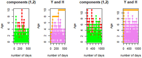
Figure 4. Final altitude $Y^{\left(1\right)}$, $Y^{\left(2\right)}$, and Y and height H of a TDMW with lengths 500 and 1000 for $p_0=p=1/8$ and $p_1=p_2=3/8$.

Figure 5 shows that if the length of the random walk is equal to 10, the final altitudes of $Y^{\left(1\right)}$ and $Y^{\left(2\right)}$ are equal to 3 and 0; then, the maximum altitude Y is 3, and the height H is 5. When the length of the walk is increased from 10 to 100, we remark that the final altitudes of $Y^{\left(1\right)}$, $Y^{\left(2\right)}$, and Y change a little and are equal to at most 2, and the final altitude of the height H is equal to 3. Then, the difference in the final altitude of the height is very small, ranging from three to five between the two lengths of the walk and being bounded by 5.

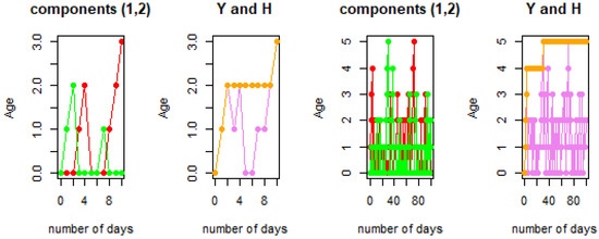
Figure 5. Final altitude $Y^{\left(1\right)}$, $Y^{\left(2\right)}$, and Y and height H of the Moran walk with lengths 10 and 100 for $p_0=p=1/6$ and $p_1=p_2=1/3$.

Figure 6 shows that the final altitude of $Y^{\left(1\right)}$, $Y^{\left(2\right)}$, and Y is equal to at most 4, and the final altitude of the height H is fixed at 10 for the Moran walk of length 500. When the length is increased from 500 to 1000, we observe that the final altitudes of $Y^{\left(1\right)}$, $Y^{\left(2\right)}$, and Y are moved a little and at most are equal to 6, and the final altitude of the height H is fixed at 11. It is clear that the height is bounded by eight by eleven. The maximum age of the two components is at most equal to 11.

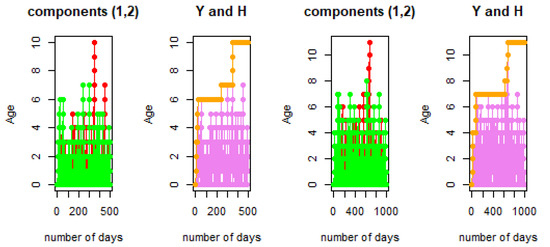
Figure 6. Final altitude $Y^{\left(1\right)}$, $Y^{\left(2\right)}$, and Y and height H of a TDMW with lengths 500 and 1000 for $p_0=p=1/6$ and $p_1=p_2=1/3$.

5. Recursive Equations

In this section, we first calculate the probability of the process defined in (6), denoted by $P_{n+1}(k_1,k_2)$ at time $n+1$ given that we know it at time n. Secondly, we study the sequence of multivariate polynomials, denoted by $f_n(x_1,x_2)$, and find the recursive equation related to this sequence between two consecutive times n and $n+1$. Next, we investigate the probability generating function, denoted by $F(t,x_1,x_2)$, for our model. Finally, we prove that the limiting distribution of each component converges to the shifted geometric distribution and calculate their means and variances. Applying the fifth definition in Section 2, we then have the following definition: for all $k_1$, $k_2\in \{0,\dots ,n+1\}$,

$$\begin{array}{cc}\hfill P_{n+1}(k_1,k_2)=& P\left(Y_{n+1}^{\left(1\right)}=k_1,Y_{n+1}^{\left(2\right)}=k_2\right)\hfill \\ \hfill =& P\left(Y_{n+1}^{\left(1\right)}=k_1,Y_{n+1}^{\left(2\right)}=k_2|Y_n^{\left(1\right)}=l,Y_n^{\left(2\right)}=q\right),\hfill \end{array}$$

(9)

where $l,q\in \{0,\dots ,n\}$. We start this section with a technical lemma. It leads to the involvement of a recursive equation between the probability of our model for two consecutive times n and $n+1$, and it will be used in Theorem 3. It is based on the following conditional probability: consider two events A and B, where the probability of event A occurs given that event B occurred in the past, given by

$${\displaystyle P\left(A\right|B)=\frac{P(A\cap B)}{P\left(B\right)},}$$

where the probability of B is strictly positive. It is presented by the following lemma:

Lemma 2. 

We have the following recursion of probabilities:

$$\begin{array}{cc}\hfill P_{n+1}(k_1,k_2)& =\left\{\begin{array}{cc}p{P}_n(k_1-1,k_2-1),\hfill & \mathrm{if}{k}_1\ge 1,k_2\ge 1,\hfill \\ p_1\sum _{l=0}^n{P}_n(l,k_2-1),\hfill & \mathrm{if}{k}_1=0,k_2\ge 1,\hfill \\ p_2\sum _{q=0}^n{P}_n(k_1-1,q),\hfill & \mathrm{if}{k}_1\ge 1,k_2=0,\hfill \\ p_0\sum _{k_1=0}^n\sum _{k_2=0}^n{P}_n(k_1,k_2),\hfill & \mathrm{if}{k}_1=0,k_2=0.\hfill \end{array}\right.\hfill \end{array}$$

Proof. 

This proof is based on the utility of the conditional probability that the Moran walks $Y^{\left(1\right)}$ and $Y^{\left(2\right)}$ are aged $k_1$ and $k_2$ at time $n+1$ given that they are aged l and q at time n; thus, For $k_1\ge 1$ and $k_2\ge 1$, we have

$$\begin{array}{ccc}\hfill P_{n+1}(k_1,k_2)& =& P(Y_{n+1}^{\left(1\right)}=k_1,Y_{n+1}^{\left(2\right)}=k_2)\hfill \\ & =& P(Y_n^{\left(1\right)}+1=k_1,Y_n^{\left(2\right)}+1=k_2,Y_n^{\left(1\right)}=k_1-1,Y_n^{\left(2\right)}=k_2-1)\hfill \\ & =& P(Y_n^{\left(1\right)}+1=k_1,Y_n^{\left(2\right)}+1=k_2|Y_n^{\left(1\right)}=k_1-1,Y_n^{\left(2\right)}=k_2-1)\hfill \\ & & \times P(Y_n^{\left(1\right)}=k_1-1,Y_n^{\left(2\right)}=k_2-1)\hfill \\ & =& p{P}_n(k_1-1,k_2-1).\hfill \end{array}$$

For $k_1=0$ and $k_2\ge 1$, we have:

$$\begin{array}{ccc}\hfill P_{n+1}(k_1,k_2)& =& {\displaystyle \sum _{l=0}^{n}P(Y_n^{\left(1\right)}+1=0,Y_n^{\left(2\right)}+1=k_2,Y_n^{\left(1\right)}=l,Y_n^{\left(2\right)}=k_2-1)}\hfill \\ & =& {\displaystyle p_1\sum _{l=0}^n{P}_n(l,k_2-1).}\hfill \end{array}$$

For $k_1\ge 1$ and $k_2=0$, we have by symmetry:

$$\begin{array}{ccc}\hfill P_{n+1}(k_1,k_2)& =& {\displaystyle \sum _{q=0}^{n}P(Y_n^{\left(1\right)}+1=k_1,Y_n^{\left(2\right)}+1=0,Y_n^{\left(1\right)}=k_1-1,Y_n^{\left(2\right)}=q)}\hfill \\ & =& {\displaystyle \sum _{q=0}^{n}P(Y_n^{\left(1\right)}+1=k_1,Y_n^{\left(2\right)}+1=0|Y_n^{\left(1\right)}=k_1-1,Y_n^{\left(2\right)}=q)}\hfill \\ & & {\displaystyle \times P(Y_n^{\left(1\right)}=k_1-1,Y_n^{\left(2\right)}=q)=p_2\sum _{q=0}^n{P}_n(k_1-1,q).}\hfill \end{array}$$

For $k_1=k_2=0$, we have:

$$\begin{array}{ccc}\hfill P_{n+1}(0,0)& =& {\displaystyle P(Y_n^{\left(1\right)}+1=0,Y_n^{\left(2\right)}+1=0,Y_n^{\left(1\right)}=0,Y_n^{\left(2\right)}=0)}\hfill \\ & & {\displaystyle +\sum _{l=1}^{n}P(Y_n^{\left(1\right)}+1=0,Y_n^{\left(2\right)}+1=0,Y_n^{\left(1\right)}=l,Y_n^{\left(2\right)}=0)}\hfill \\ & & {\displaystyle +\sum _{q=1}^{n}P(Y_n^{\left(1\right)}+1=0,Y_n^{\left(2\right)}+1=0,Y_n^{\left(1\right)}=0,Y_n^{\left(2\right)}=q)}\hfill \\ & & {\displaystyle +\sum _{l,q=1}^{n}P(Y_n^{\left(1\right)}+1=0,Y_n^{\left(2\right)}+1=0,Y_n^{\left(1\right)}=l,Y_n^{\left(2\right)}=q)}\hfill \\ & =& {\displaystyle p_0\left(P_n(k_1,k_2)+\sum _{q=1}^n{P}_n(0,q)+\sum _{l=1}^n{P}_n(l,0)+\sum _{l,q=1}^n{P}_n(l,q)\right)}\hfill \\ & =& {\displaystyle p_0\sum _{k_1=0}^n\sum _{k_2=0}^n{P}_n(k_1,k_2)=p_0.}\hfill \end{array}$$

□

Remark 2. 

We offer some comments on the different cases of the age of the two components $Y_{n+1}^{\left(1\right)}$ and $Y_{n+1}^{\left(2\right)}$:

1. 

In the first case, if the two final ages of the two components are equal to at least one, then the probability that the two components are aged $k_1$ and $k_2$ at time $n+1$ is equal to p multiplied by the probability of two components that are aged $k_1-1$ and $k_2-1$ at time n.

2. 

In the second case, if the ages of the two components one and two are equal to zero and at least one at time $n+1$, then the probability that the two components are aged $k_1=0$ and $k_2$ at time $n+1$ is equal to $p_1$ multiplied by the sum of probabilities such that the two components are aged l, which is started from 0 to n and $k_2-1$ at time n, respectively.

3. 

In the third case, if the ages of two components two and one are equal to zero and at least one at time $n+1$, then the probability that the two components are aged $k_2=0$ and $k_1$ at time $n+1$ is equal to $p_2$ multiplied by the sum of probabilities such that the two components are aged q, which is started from 0 to n and $k_1-1$ at time n, respectively.

4. 

In the fourth case, if the ages of two components one and two are equal to zero, then the probability that the two components are aged $k_2=0$ and $k_1=0$ at time $n+1$ is equal to $p_0$ multiplied by the double sum of the probabilities such that the two components are aged l and q starting from zero to n at time n, respectively.

In the next section, we define the sequence of multivariate polynomials $f_n(x_1,x_2)$ (for $n\in \mathbb{N}$) by the fact that the coefficient of $x_1^{k_1}{x}_2^{k_2}$ in $f_n(x_1,x_2)$ is the probability that, at time n, the i-th individual has age $k_i$ (for $i=1,2$); that is,

$${\displaystyle f_n(x_1,x_2)=\mathbb{E}\left(x_1^{Y_n^{\left(1\right)}}{x}_2^{Y_n^{\left(2\right)}}\right)=\sum _{k_1=0}^n\sum _{k_2=0}^n{x}_1^{k_1}{x}_2^{k_2}{P}_n(k_1,k_2).}$$

(10)

Starting from Equation (10) and using the preceding lemma, we can find a recursive equation that is related between $f_{n+1}(x_1,x_2)$, $f_n(x_1,1)$, $f_n(1,x_2)$, and $f_n(x_1,x_2)$; it is introduced in the next proposition.

Proposition 1. 

For all $x_1,x_2\in \mathbb{R}$, the sequence of multivariate polynomials $f_n(x_1,x_2)$ satisfies the recursive equation:

$${\displaystyle f_{n+1}(x_1,x_2)=p_0{f}_n(1,1)+p_1{x}_2{f}_n(1,x_2)+p_2{x}_1{f}_n(x_1,1)+p{x}_1{x}_2{f}_n(x_1,x_2),}$$

(11)

with initial condition ${\displaystyle f_0(x_1,x_2)=P_0(0,0)=1}$.

Proof. 

Using Equation (10) and Lemma 2, we have

$$\begin{array}{ccc}\hfill f_{n+1}(x_1,x_2)=P_{n+1}(0,0)& +& \underset{A}{\underbrace{\sum _{k_1=1}^{n+1}\sum _{k_2=1}^{n+1}{x}_1^{k_1}{x}_2^{k_2}{P}_{n+1}(k_1,k_2)}}\hfill \\ & +& \underset{B}{\underbrace{\sum _{k_1=1}^{n+1}{x}_1^{k_1}{P}_{n+1}(k_1,0)}}+\underset{C}{\underbrace{\sum _{k_2=1}^{n+1}{x}_2^{k_2}{P}_{n+1}(0,k_2)}}.\hfill \end{array}$$

(12)

By a simple calculation, we have

$$\begin{array}{ccc}\hfill {\displaystyle A}& =& {\displaystyle p\sum _{k_1=1}^{n+1}\sum _{k_2=1}^{n+1}{x}_1^{k_1}{x}_2^{k_2}{P}_n(k_1-1,k_2-1)}\hfill \\ & =& {\displaystyle p{x}_1{x}_2\sum _{k_1=0}^n\sum _{k_2=0}^n{x}_1^{k_1}{x}_2^{k_2}{P}_n(k_1,k_2)=p{x}_1{x}_2{f}_n(x_1,x_2),}\hfill \end{array}$$

(13)

$$\begin{array}{c}\hfill {\displaystyle C=\sum _{k_2=1}^{n+1}{x}_2^{k_2}\sum _{l=0}^n{P}_n(l,k_2-1)=p_1{x}_2\sum _{k_2=0}^n{x}_2^{k_2}\sum _{l=0}^n{P}_n(l,k_2)=p_1{x}_2{f}_n(1,x_2).}\end{array}$$

(14)

By symmetry, we have

$$\begin{array}{c}\hfill {\displaystyle B=\sum _{k_1=1}^{n+1}{x}_1^{k_1}{p}_2\sum _{q=0}^n{P}_n(k_1-1,q)=p_2{x}_1\sum _{k_1=0}^n{x}_1^{k_1}\sum _{q=0}^n{P}_n(k_1,q)=p_2{x}_1{f}_n(x_1,1),}\end{array}$$

(15)

and

$$\begin{array}{ccc}\hfill {\displaystyle P_{n+1}(0,0)}& =& {\displaystyle p_0\sum _{k_1=0}^n\sum _{k_2=0}^{n}P(Y_n^{\left(1\right)}=k_1,Y_n^{\left(2\right)}=k_2)}\hfill \\ & =& {\displaystyle p_0\sum _{k_1=0}^n\sum _{k_2=0}^n{1}_1^{k_1}{1}_2^{k_2}P(Y_n^{\left(1\right)}=k_1,Y_n^{\left(2\right)}=k_2)=p_0{f}_n(1,1).}\hfill \end{array}$$

(16)

We conclude the proof through the combination of Equations (12)–(16). □

6. Distributions of ${\mathit{Y}}_{\mathit{n}}^{\left(\mathbf{1}\right)}$ and ${\mathit{Y}}_{\mathit{n}}^{\left(\mathbf{2}\right)}$

In this section, we study some statistical characteristics such as the probability generating function, the asymptotic distribution, the mean, and the variance of the final altitude of each component $Y_n^{\left(1\right)}$ and $Y_n^{\left(2\right)}$ at time n. Precisely, we start to find the probability generating function of each component as denoted by $f_n(x_1,1)$ and $f_n(1,x_2)$. In the next theorem, we prove that the final altitude of each component converges to the shifted geometric distribution in the law. This partially generalizes the results of Itoh and Mahmoud [10] (which was restricted to the uniform case, i.e., $p_1=p_2$, but in any dimension). Finally, we finish this section by calculating the mean and variance of each component. The following theorem that is presented is the probability generating function and asymptotic limit of $Y_n^{\left(1\right)}$ and $Y_n^{\left(2\right)}$.

Theorem 3. 

The distributions of $Y_n^{\left(1\right)}$ and $Y_n^{\left(2\right)}$ follow the same discrete distribution, with probability generating functions being given by: $\forall (x_1,x_2)\in {\mathbb{R}}^2$

$$\left\{\begin{array}{c}{\displaystyle f_0(x_1,x_2)=1,}\hfill \\ {\displaystyle f_n(x_1,1)={\left(r_1{x}_1\right)}^n+(1-r_1)\frac{1-{\left(r_1{x}_1\right)}^n}{1-r_1{x}_1},}\hfill \\ {\displaystyle f_n(1,x_2)={\left(r_2{x}_2\right)}^n+(1-r_2)\frac{1-{\left(r_2{x}_2\right)}^n}{1-r_2{x}_2}.}\hfill \end{array}\right.$$

Asymptotically, $Y_n^{\left(1\right)}$ and $Y_n^{\left(2\right)}$ converge, in law, to some shifted geometric (Geo) random variables:

$$Y_n^{\left(1\right)}⟶Geo(1-r_1)-1and{Y}_n^{\left(2\right)}⟶Geo(1-r_2)-1,$$

where $r_1=p_2+p$, $r_2=p_1+p$, $|r_1{x}_1|<1$ and $|r_2{x}_2|<1$.

Proof. 

Using the recursive equation defined in (11) for $x_2=1$, we get

$$\begin{array}{ccc}\hfill f_{n+1}(x_1,1)& =& (p_0+p_1)f_n(1,1)+(p+p_2)x_1{f}_n(x_1,1)\hfill \\ & =& {\displaystyle (1-r_1)\sum _{k=0}^n{\left(x_1{r}_1\right)}^k{f}_{n-k}(1,1)+{\left(r_1{x}_1\right)}^{n+1}}\hfill \\ & =& {\left(r_1{x}_1\right)}^{n+1}+(1-r_1)\frac{1-{\left(r_1{x}_1\right)}^{n+1}}{1-r_1{x}_1}.\hfill \end{array}$$

By symmetry, we have

$$f_{n+1}(1,x_2)={\left(r_2{x}_2\right)}^{n+1}+(1-r_2)\frac{1-{\left(r_2{x}_2\right)}^{n+1}}{1-r_2{x}_2}.$$

Passing to the limit of $f_{n+1}(x_1,1)$, we then have

$${\displaystyle \underset{n\to \infty }{lim}{f}_n(x_1,1)=\underset{n\to \infty }{lim}\left({\left(r_1{x}_1\right)}^n+(1-r_1)\frac{1-{\left(r_1{x}_1\right)}^n}{1-r_1{x}_1}\right)=\frac{1-r_1}{1-r_1{x}_1}.}$$

(17)

Suppose that Z follows the geometric distribution with parameter $1-r_1$. Then, its probability is given by

$${\displaystyle P(Z=k)=(1-r_1)r_1^{k-1},\forall k\ge 0}$$

and the probability generating function of Z is equal to

$${\displaystyle G_Z\left(x_1\right)=(1-r_1)\sum _{k=0}^{\infty }{r}_1^k{x}_1^k=\frac{1-r_1}{1-r_1{x}_1},if\left|r_1{x}_1\right|<1.}$$

(18)

The relations (17) and (18) prove that $Y^{\left(1\right)}$ converges to $geo(1-r_1)-1$ in the distribution. □

From Theorem 3, we directly get the following corollary concerning the explicit expressions of the means and variances of $Y_n^{\left(1\right)}$ and $Y_n^{\left(2\right)}$, which depend on probability generating functions.

Corollary 1. 

The mean and variance of the final altitude $Y_n$ of each component of Moran walk ${\left(Y_n^{\left(i\right)}\right)}_{i=1,2}$ are given by:

$$\begin{array}{ccc}\hfill {\displaystyle \mathbb{E}\left(Y_n^{\left(i\right)}\right)=\frac{r_i-r_i^{n+1}}{1-r_i}and\mathbb{V}\mathrm{ar}\left(Y_n^{\left(i\right)}\right)}& =& {\displaystyle \frac{r_i}{{(1-r_i)}^2}\left(1-r_i^n\left[r_i^{n+1}+(1+2n)(1-r_i)\right]\right),}\hfill \end{array}$$

where $r_1=p_2+p$, $r_2=p_1+p$, $|r_1{x}_1|<1$ and $|r_2{x}_2|<1$.

Proof. 

Calculating the first derivative of $f_n(x_1,1)$ with respect to $x_1$,

$$\begin{array}{ccc}\hfill \frac{\partial f_n(x_1,1)}{\partial x_1}& =& {\displaystyle \frac{\partial }{\partial x_1}\left\{n{r}_1^n{x}_1^{n-1}+(1-r_1)\frac{-n{r}_1^n{x}_1^{n-1}\left(1-r_1{x}_1\right)+r_1\left(1-r_1^n{x}_1^n\right)}{{\left(1-r_1{x}_1\right)}^2}\right\},}\hfill \end{array}$$

evaluating at $x_1=1$,

$$\begin{array}{c}\hfill {\displaystyle \frac{\partial f_n(x_1,1)}{\partial x_1}{|}_{x_1=1}=n{r}_1^n+(1-r_1)\frac{-n{r}_1^n(1-r_1)+r_1(1-r_1^n)}{{(1-r_1)}^2}=\frac{r_1-r_1^{n+1}}{1-r_1},}\end{array}$$

and using Equation (5) we get

$${\displaystyle \mathbb{E}\left(Y_n^{\left(1\right)}\right)=\frac{\partial f_n(x_1,1)}{\partial x_1}{|}_{x_1=1}=\frac{r_1-r_1^{n+1}}{1-r_1}.}$$

(19)

By symmetry, the mean of $Y_n^{\left(2\right)}$ is given by

$$\begin{array}{c}\hfill {\displaystyle \mathbb{E}\left(Y_n^{\left(2\right)}\right)=\frac{\partial f_n(1,x_2)}{\partial x_2}{|}_{x_2=1}=\frac{r_2-r_2^{n+1}}{1-r_2}.}\end{array}$$

Computing the second derivative of $f_n(x_1,1)$ with respect to $x_1$, one has

$$\begin{array}{ccc}\hfill \frac{{\partial }^2{f}_n(x_1,1)}{{\partial }^2{x}_1}& =& {\displaystyle \frac{\partial }{\partial x_1}\left\{n{r}_1^n{x}_1^{n-1}+(1-r_1)\frac{-n{r}_1^n{x}_1^{n-1}\left(1-r_1{x}_1\right)+r_1\left(1-r_1^n{x}_1^n\right)}{{\left(1-r_1{x}_1\right)}^2}\right\}}\hfill \\ & =& n(n-1)r_1^n{x}_1^{n-2}-n(1-r_1)r_1^n\left\{\frac{(n-1)x_1^{n-2}}{1-r_1{x}_1}+r_1\frac{x_1^{n-1}}{{(1-r_1{x}_1)}^2}\right\}\hfill \\ & & +r_1(1-r_1)\left\{\frac{-n{r}_1^n{x}_1^{n-1}}{{(1-r_1{x}_1)}^2}+2r_1\frac{1-r_1^n{x}_1^n}{{(1-r_1{x}_1)}^3}\right\},\hfill \end{array}$$

and evaluating at $x_1=1$, one has

$$\begin{array}{cc}\hfill \frac{{\partial }^2{f}_n(x_1,1)}{{\partial }^2{x}_1}{|}_{x_1=1}=& n(n-1)r_1^n-n(1-r_1)r_1^n\left\{\frac{(n-1)}{1-r_1}+r_1\frac{1}{{(1-r_1)}^2}\right\}\hfill \\ \hfill & +r_1(1-r_1)\left\{\frac{-n{r}_1^n}{{(1-r_1)}^2}+2r_1\frac{1-r_1^n}{{(1-r_1)}^3}\right\}\hfill \\ \hfill =& \frac{-2n{r}_1^{n+1}}{(1-r_1)}+\frac{2r_1^2(1-r_1^n)}{{(1-r_1)}^2}.\hfill \end{array}$$

(20)

Using Equations (5), (19) and (20), the variance is then given by

$$\begin{array}{cc}\hfill \mathbb{V}\mathrm{ar}\left(Y_n^{\left(1\right)}\right)=& \frac{-2n{r}_1^{n+1}}{(1-r_1)}+\frac{2r_1^2(1-r_1^n)}{{(1-r_1)}^2}+\frac{r_1-r_1^{n+1}}{(1-r_1)}-{\left(\frac{r_1-r_1^{n+1}}{1-r_1}\right)}^2\hfill \\ \hfill =& \frac{r_1}{{(1-r_1)}^2}\left(1-r_1^n\left\{r_1^{n+1}+(1+2n)(1-r_1)\right\}\right).\hfill \end{array}$$

By symmetry, we have

$$\begin{array}{ccc}\hfill \mathbb{V}\mathrm{ar}\left(Y_n^{\left(2\right)}\right)& =& {\displaystyle \frac{r_2}{{(1-r_2)}^2}\left(1-r_2^n\left\{r_2^{n+1}+(1+2n)(1-r_2)\right\}\right).}\hfill \end{array}$$

□

7. Proofs

In this section, we prove Theorems 1 and 2 of our main result. For this purpose, consider the three sequences of polynomials, $R_n\left(x\right)$, $A_n\left(x\right)$, and $S_n\left(x\right)$, which are defined by

$$\begin{array}{ccc}\hfill {\displaystyle R_n\left(x\right)}& =& {\displaystyle \sum _{k=1}^n\sum _{l=1}^k{x}^{k}P\left(Y_n^{\left(1\right)}=k,Y_n^{\left(2\right)}=l\right),R_0\left(x\right)=0}\hfill \end{array}$$

(21)

$$\begin{array}{ccc}\hfill {\displaystyle A_n\left(x\right)}& =& {\displaystyle \sum _{k=0}^n\sum _{l=k+1}^n{x}^{k}P\left(Y_n^{\left(1\right)}=k,Y_n^{\left(2\right)}=l\right),A_0\left(x\right)=0,}\hfill \end{array}$$

(22)

$$\begin{array}{ccc}\hfill {\displaystyle S_n\left(x\right)}& =& {\displaystyle \sum _{k=0}^n\sum _{l=0}^k{x}^{k}P\left(Y_n^{\left(1\right)}=k,Y_n^{\left(2\right)}=l\right),S_0\left(x\right)=1.}\hfill \end{array}$$

(23)

The following lemmas are technical and will be used for the proof of Theorem 1. The first lemma is used to calculate $A_n\left(x\right)$ when the final age of the first component can be equal to zero but the final age of the second component two is increased by one unit more than the first. It is presented by:

Lemma 3. 

The sequence ${\displaystyle A_n\left(x\right)}$ satisfies the recursive equation

$${\displaystyle A_n\left(x\right)=p_1+px{A}_{n-1}\left(x\right)=p_1\frac{1-{\left(px\right)}^n}{1-px},}$$

for all $n\in {\mathbb{N}}^{*}$ and for all $x\in \mathbb{R}$, such that $\left|px\right|<1$.

Proof. 

We can write ${\displaystyle A_n\left(x\right)}$ by

$$\begin{array}{ccc}\hfill {\displaystyle A_n\left(x\right)}& =& {\displaystyle \sum _{l=1}^{n}P\left(Y_n^{\left(1\right)}=0,Y_n^{\left(2\right)}=l\right)+\sum _{k=1}^n\sum _{l=k+1}^n{x}^{k}P\left(Y_n^{\left(1\right)}=k,Y_n^{\left(2\right)}=l\right),}\hfill \end{array}$$

and using Lemma 2, we obtain

$$\begin{array}{ccc}\hfill A_n\left(x\right)& =& {\displaystyle p_1{f}_{n-1}(1,1)+\sum _{k=1}^n\sum _{l=k+1}^n{x}^{k}P\left(Y_n^{\left(1\right)}=k,Y_n^{\left(2\right)}=l\right)}\hfill \\ & =& {\displaystyle p_1+px\sum _{k=0}^{n-1}\sum _{l=k+1}^{n-1}{x}^{k}P\left(Y_{n-1}^{\left(1\right)}=k,Y_{n-1}^{\left(2\right)}=l\right)}\hfill \\ & =& {\displaystyle p_1+px{A}_{n-1}\left(x\right).}\hfill \end{array}$$

Iterating n times $A_n\left(x\right)$, we get

$${\displaystyle A_n\left(x\right)=p_1\sum _{r=0}^{n-1}{\left(px\right)}^r=p_1\frac{1-{\left(px\right)}^n}{1-px}.}$$

□

We use the previous lemma to find a recursive equation for the sequence $R_n\left(x\right)$. It depends on the probability generating function of the walk $Y_n^{\left(1\right)}$ and sequence $A_n$. The second lemma in this section is used to calculate $R_n\left(x\right)$ when the final ages of the two components can be equal and can be started from $(1,1)$ but the age of the first component does not pass the age of the first; it is presented by:

Lemma 4. 

The sequence ${\displaystyle R_n\left(x\right)}$ satisfies the recursive equation

$${\displaystyle R_n\left(x\right)=px{f}_{n-1}(x,1)-px{A}_{n-1}\left(x\right),}$$

for all $n\in {\mathbb{N}}^{*}$ and for all $x\in \mathbb{R}$, such that $\left|px\right|<1$.

Proof. 

Using Lemma 2, we get

$$\begin{array}{ccc}\hfill R_n\left(x\right)& =& {\displaystyle p\sum _{k=1}^n\sum _{l=1}^k{x}^{k}P\left(Y_{n-1}^{\left(1\right)}=k-1,Y_{n-1}^{\left(2\right)}=l-1\right)}\hfill \\ & =& {\displaystyle px{f}_{n-1}(x,1)-px\sum _{k=0}^{n-1}\sum _{l=k+1}^{n-1}{x}^{k}P\left(Y_{n-1}^{\left(1\right)}=k,Y_{n-1}^{\left(2\right)}=l\right)}\hfill \\ & =& {\displaystyle px{f}_{n-1}(x,1)-px{A}_{n-1}\left(x\right).}\hfill \end{array}$$

□

We will use Lemma 4 to find a recursive equation for the sequence $S_n\left(x\right)$; it depends on the probability generating function of the walk $Y_n^{\left(1\right)}$ and sequence $A_n$. The following lemma is used to calculate $S_n\left(x\right)$ when the final ages of the two components can be equal and can be started from $(0,0)$ but the age of the second component does not pass the age of the first; it is presented in the following lemma.

Lemma 5. 

The sequence $S_n\left(x\right)$ satisfies the recursive equation:

$${\displaystyle S_n\left(x\right)=p_0+(p+p_2)x{f}_{n-1}(x,1)-px{A}_{n-1}\left(x\right),}$$

and $S_n\left(x\right)$ is given exactly by

$$S_n\left(x\right)=p_0-p_1\frac{px-{\left(px\right)}^n}{1-px}+{\left(r_{1}x\right)}^n+(1-r_1)\frac{r_{1}x-{\left(r_{1}x\right)}^n}{1-r_{1}x}.$$

(24)

for all $x\in \mathbb{R}$ such that $\left|px\right|<1$ and $|r_{1}x|<1$, where $r_1$ is defined in Theorem 3.

Proof. 

Developing the sequence $S_n\left(x\right)$

$$\begin{array}{cc}\hfill {\displaystyle S_n\left(x\right):=}& {\displaystyle \sum _{k=0}^n\sum _{l=0}^k{x}^{k}P\left(Y_n^{\left(1\right)}=k,Y_n^{\left(2\right)}=l\right)}\hfill \\ \hfill =& {\displaystyle P\left(Y_n^{\left(1\right)}=0,Y_n^{\left(2\right)}=0\right)+\sum _{k=1}^n{x}^{k}P\left(Y_n^{\left(1\right)}=k,Y_n^{\left(2\right)}=0\right)}\hfill \\ \hfill & {\displaystyle +\sum _{l=1}^k{x}^{k}P\left(Y_n^{\left(1\right)}=0,Y_n^{\left(2\right)}=l\right)+\sum _{k=1}^n\sum _{l=1}^k{x}^{k}P\left(Y_n^{\left(1\right)}=k,Y_n^{\left(2\right)}=l\right),}\hfill \end{array}$$

and using Lemma 2 and Equation (10), we have

$$P\left(Y_n^{\left(1\right)}=0,Y_n^{\left(2\right)}=0\right)=P_n(0,0)=p_0,$$

(25)

$$\sum _{k=1}^n{x}^{k}P\left(Y_n^{\left(1\right)}=k,Y_n^{\left(2\right)}=0\right)=p_{2}x{f}_{n-1}(x,1),$$

(26)

and

$$\sum _{l=1}^{k=0}{x}^{k}P\left(Y_n^{\left(1\right)}=0,Y_n^{\left(2\right)}=l\right)=0.$$

(27)

Combining Equations (21) and (25)–(27), we get

$$\begin{array}{cc}\hfill {\displaystyle S_n\left(x\right)=}& {\displaystyle p_0+p_{2}x{f}_{n-1}(x,1)+A_n\left(x\right)}\hfill \\ \hfill =& {\displaystyle p_0+\left(p_2+p\right)x{f}_{n-1}(x,1)-p_1\frac{px-{\left(px\right)}^n}{1-px},}\hfill \end{array}$$

and using the expression of $f_{n-1}(x,1)$ defined in Theorem 3, we obtain the formula of $S_n\left(x\right)$ defined in (24). □

Remark 3. 

Consider the sequence $L_n\left(x\right)$ given by the following: for all $n\in \mathbb{N}$,

$$L_0\left(x\right)=1,L_n\left(x\right):=\sum _{k=0}^n\sum _{l=0}^k{x}^{k}P\left(Y_n^{\left(1\right)}=l,Y_n^{\left(2\right)}=k\right),$$

calculate the sum of $x^{k}P\left(Y_n^{\left(1\right)}=l,Y_n^{\left(2\right)}=k\right)$ under the condition that the final ages of the two components can be equal and can be started from $(0,0)$ but the age of the first component does not pass the age of the second.

We observe that the two sequences $L_n\left(x\right)$ and $S_n\left(x\right)$ are symmetric; thus, the expression of ${\displaystyle L_n\left(x\right)}$ is directly given by the following: for all $n\in {\mathbb{N}}^{*}$, for all $x\in \mathbb{R}$ such that $\left|px\right|<1$ and $|r_{2}x|<1$,

$$\begin{array}{c}\hfill {\displaystyle L_n\left(x\right)=p_0+\left({\left(r_{2}x\right)}^n+(1-r_2)\frac{r_{2}x-{\left(r_{2}x\right)}^n}{1-r_{2}x}\right)-p_2\frac{px-{\left(px\right)}^n}{1-px},}\end{array}$$

(28)

where $r_2$ is defined in Theorem 3.

Consider the sequence $C_n\left(x\right)$ given by: for all $n\in \mathbb{N}$, for all $x\in \mathbb{R}$,

$${\displaystyle C_n\left(x\right)=\sum _{k=0}^n{x}^{k}P\left(Y_n^{\left(1\right)}=k,Y_n^{\left(2\right)}=k\right).}$$

(29)

The following lemma is used to calculate $C_n\left(x\right)$ when the final ages of two components are equal and are started from $(0,0)$; it is presented by the following:

Lemma 6. 

The sequence ${\displaystyle C_n\left(x\right)}$ satisfies the recursive equation: for all $n\in \mathbb{N}$ such that $\left|px\right|<1$,

$${\displaystyle C_n\left(x\right)=p_0+px{C}_{n-1}\left(x\right)=p_0\frac{1-{\left(px\right)}^n}{1-px}+{\left(px\right)}^n.}$$

Proof. 

Rewriting $C_n\left(x\right)$

$$\begin{array}{ccc}\hfill {\displaystyle C_n\left(x\right)}& =& {\displaystyle \sum _{k=0}^n{x}^{k}P\left(Y_n^{\left(1\right)}=k,Y_n^{\left(2\right)}=k\right)}\hfill \\ & =& {\displaystyle P_n(0,0)+\sum _{k=1}^n{x}^{k}P\left(Y_n^{\left(1\right)}=k,Y_n^{\left(2\right)}=k\right),}\hfill \end{array}$$

and using Lemma 2 and Equation (10), we obtain

$$\begin{array}{ccc}\hfill {\displaystyle C_n\left(x\right)}& =& {\displaystyle p_0{f}_{n-1}(1,1)+p\sum _{k=1}^n{x}^{k}P\left(Y_{n-1}^{\left(1\right)}=k-1,Y_{n-1}^{\left(2\right)}=k-1\right)}\hfill \\ & =& {\displaystyle p_0+px\sum _{k=0}^{n-1}{x}^{k}P\left(Y_{n-1}^{\left(1\right)}=k,Y_{n-1}^{\left(2\right)}=k\right)}\hfill \\ & =& {\displaystyle p_0+px{C}_{n-1}\left(x\right).}\hfill \end{array}$$

Iterating n times $C_n\left(x\right)$ and getting $\forall n\in \mathbb{N}$, $\forall x\in \mathbb{R}$ such that $\left|px\right|<1$, one has

$$C_n\left(x\right)=p_0\sum _{r=0}^{n-1}{\left(px\right)}^r+{\left(px\right)}^n=p_0\frac{1-{\left(px\right)}^n}{1-px}+{\left(px\right)}^n.$$

(30)

□

The last lemma gives the probability that the two components have age $k\ge 0$.

Corollary 2. 

For all $k\in \mathbb{N}$, we have

$$P(Y_n^{\left(1\right)}=Y_n^{\left(2\right)}=k)=\left\{\begin{array}{c}{p}_0{p}^k,ifk\in \{0,1,\dots ,n-1\},\hfill \\ p^n,ifk=n.\hfill \end{array}\right.$$

Proof. 

Identifying Equations (29) and (30), we have

$$C_n\left(x\right)=p_0\sum _{r=0}^{n-1}{\left(px\right)}^r+{\left(px\right)}^n=\sum _{k=0}^{n-1}{x}^{k}P\left(Y_n^{\left(1\right)}=k,Y_n^{\left(2\right)}=k\right)+P\left(Y_n^{\left(1\right)}=Y_n^{\left(2\right)}=n\right)x^n,$$

which finishes the proof. □

Here, we present the proof of Theorem 1, which is based on the four previous lemmas.

7.1. Proof of Theorem 1

We have

$$\begin{array}{ccc}\hfill {\Psi }_n\left(x\right)& =& {\displaystyle \sum _{k=0}^n{x}^{k}P(Y_n=k)=\sum _{k=0}^n{x}^{k}P\left(max(Y_n^{\left(1\right)},Y_n^{\left(2\right)})=k\right)}\hfill \\ & =& {\displaystyle \sum _{k=0}^n{x}^k\left(P(Y_n^{\left(1\right)}=k,Y_n^{\left(2\right)}\le k)+P(Y_n^{\left(1\right)}<k,Y_n^{\left(2\right)}=k)\right)}\hfill \\ & =& {\displaystyle \sum _{k=0}^n\sum _{l=0}^k{x}^{k}P(Y_n^{\left(1\right)}=k,Y^{\left(2\right)}=l)+\sum _{k=0}^n\sum _{l=0}^k{x}^{k}P(Y_n^{\left(1\right)}=l,Y_n^{\left(2\right)}=k)}\hfill \\ & & {\displaystyle -\sum _{k=0}^n{x}^{k}P(Y_n^{\left(1\right)}=k,Y_n^{\left(2\right)}=k)=S_n(x)+L_n(x)-C_n(x).}\hfill \end{array}$$

Using the results in Lemma 5, Remark 3, and Lemma 6, we get

$$\begin{array}{ccc}\hfill {\displaystyle {\Psi }_n\left(x\right)}& =& {\displaystyle p_0-p_1\frac{px-{\left(px\right)}^n}{1-px}+{\left(r_{1}x\right)}^n+(1-r_1)\frac{r_{1}x-{\left(r_{1}x\right)}^n}{1-r_{1}x}}\hfill \\ & & {\displaystyle +p_0-p_2\frac{px-{\left(px\right)}^n}{1-px}+{\left(r_{2}x\right)}^n+(1-r_2)\frac{r_{2}x-{\left(r_{2}x\right)}^n}{1-r_{2}x}}\hfill \\ & & {\displaystyle -p_0\frac{1-{\left(px\right)}^n}{1-px}-{\left(px\right)}^n,}\hfill \end{array}$$

Simplifying ${\Psi }_n\left(x\right)$, we then get

$$\begin{array}{ccc}\hfill {\Psi }_n\left(x\right)& =& {\displaystyle 2p_0-\left(p_1+p_2\right)\frac{px-{\left(px\right)}^n}{1-px}+\left(r_1^n+r_2^n\right)x^n+(1-r_1)\frac{r_{1}x-{\left(r_{1}x\right)}^n}{1-r_{1}x}}\hfill \\ & & {\displaystyle +(1-r_2)\frac{r_{2}x-{\left(r_{2}x\right)}^n}{1-r_{2}x}-p_0\frac{1-{\left(px\right)}^n}{1-px}-{\left(px\right)}^n.}\hfill \end{array}$$

In the next section, we prove Theorem 2; for this purpose, we will need to perform two derivatives of the probability generating function defined in the previous theorem and take $x=1$ to obtain the mean and variance of $Y_n$ while using Equation (5).

7.2. Proof of Theorem 2

Calculating the first derivative of ${\Psi }_n\left(x\right)$ defined in Theorem 1,

$$\begin{array}{cc}\hfill \frac{\partial {\Psi }_n\left(x\right)}{\partial x}=& \frac{\partial }{\partial x}(2p_0-\left(p_1+p_2\right)\frac{px-{\left(px\right)}^n}{1-px}+\left(r_1^n+r_2^n\right)x^n\hfill \\ \hfill & +(1-r_1)\frac{r_{1}x-{\left(r_{1}x\right)}^n}{1-r_{1}x}+(1-r_2)\frac{r_{2}x-{\left(r_{2}x\right)}^n}{1-r_{2}x}-p_0\frac{1-{\left(px\right)}^n}{1-px}-{\left(px\right)}^n).\hfill \end{array}$$

Developing $\frac{\partial {\Psi }_n\left(x\right)}{\partial x}$, we have

$$\begin{array}{ccc}\hfill \frac{\partial {\Psi }_n\left(x\right)}{\partial x}& =& -(p_1+p_2)\left(\frac{p-np{\left(px\right)}^{n-1}}{1-px}+\frac{p(px-{\left(px\right)}^n)}{{(1-px)}^2}\right)+n\left(r_1^n+r_2^n\right)x^{n-1}\hfill \\ & & +(1-r_1)\left(\frac{r_1-n{r}_1{\left(r_{1}x\right)}^{n-1}}{(1-r_{1}x)}+\frac{r_1(r_{1}x-{\left(r_{1}x\right)}^n)}{{(1-r_{1}x)}^2}\right)\hfill \\ & & +(1-r_2)\left(\frac{r_2-n{r}_2{\left(r_{2}x\right)}^{n-1}}{(1-r_{2}x)}+\frac{r_2(r_{2}x-{\left(r_{2}x\right)}^n)}{{(1-r_{2}x)}^2}\right)\hfill \\ & & +p_0\left(\frac{pn{\left(px\right)}^{n-1}}{(1-px)}-\frac{p(1-{\left(px\right)}^n)}{{(1-px)}^2}\right)-np{\left(px\right)}^{n-1},\hfill \end{array}$$

(31)

and evaluating at $x=1$,

$$\begin{array}{ccc}\hfill \frac{\partial \Psi \left(x\right)}{\partial x}{|}_{x=1}& =& {\displaystyle \frac{-(p_1+p_2)}{{(1-p)}^2}\left((p-n{p}^n)(1-p)+p(p-p^n)\right)+\frac{r_1-r_1^{n+1}}{1-r_1}}\hfill \\ & & {\displaystyle +\frac{r_2-r_2^{n+1}}{1-r_2}+\frac{p_0}{{(1-p)}^2}\left(n{p}^n(1-p)-p(1-p^n)\right)-n{p}^n}\hfill \\ & =& {\displaystyle \frac{r_1-r_1^{n+1}}{1-r_1}+\frac{r_2-r_2^{n+1}}{1-r_2}+I_n,}\hfill \end{array}$$

(32)

where $I_n$ is a sequence defined by

$$\begin{array}{ccc}\hfill I_n& =& \frac{p_0}{{(1-p)}^2}\left(n{p}^n(1-p)-p(1-p^n)\right)\hfill \\ & & -\frac{p_1+p_2}{{(1-p)}^2}\left((p-n{p}^n)(1-p)+p(p-p^n)\right)-n{p}^n.\hfill \end{array}$$

By a simple calculation, we have

$$\begin{array}{c}\hfill \frac{p_0}{{(1-p)}^2}\left(n{p}^n(1-p)-p(1-p^n)\right)-n{p}^n=\frac{n{p}_0{p}^n}{(1-p)}-\frac{p{p}_0(1-p^n)}{{(1-p)}^2}-n{p}^n,\end{array}$$

(33)

$$\begin{array}{c}\frac{-(p_1+p_2)}{{(1-p)}^2}\left((p-n{p}^n)(1-p)+p(p-p^n)\right)\hfill \\ \hfill =-\frac{p(p_1+p_2)}{(1-p)}+\frac{n(p_1+p_2)p^n}{(1-p)}-\frac{p(p_1+p_2)(p-p^n)}{{(1-p)}^2},\end{array}$$

(34)

and adding relation (33) and (34), we observe that

$$\begin{array}{c}\hfill {\displaystyle \frac{n{p}_0{p}^n}{(1-p)}+\frac{n(p_1+p_2)p^n}{(1-p)}-n{p}^n=0,}\end{array}$$

hence,

$$\begin{array}{ccc}\hfill I_n& =& \frac{p_0}{{(1-p)}^2}\left(n{p}^n(1-p)-p(1-p^n)\right)\hfill \\ & & -\frac{p_1+p_2}{{(1-p)}^2}\left((p-n{p}^n)(1-p)+p(p-p^n)\right)-n{p}^n\hfill \\ & =& {\displaystyle -\frac{p{p}_0(1-p^n)}{{(1-p)}^2}-\frac{p(p_1+p_2)(p-p^n)}{{(1-p)}^2}-\frac{p(p_1+p_2)}{(1-p)}.}\hfill \end{array}$$

Taking the $\frac{1}{{(1-p)}^2}$ common factor, one has

$$\begin{array}{ccc}\hfill I_n& =& \frac{1}{{(1-p)}^2}(-p{p}_0+p_0{p}^{n+1}-p^2(p_1+p_2)\hfill \\ & & +(p_1+p_2)p^{n+1}-p(p_1+p_2)+p^2(p_1+p_2)).\hfill \end{array}$$

Simplifying $I_n$, we then obtain

$$\begin{array}{ccc}\hfill I_n& =& \frac{1}{{(1-p)}^2}\left(-p(p_0+p_1+p_2)+p^{n+1}(p_0+p_1+p_2)\right)=\frac{-p+p^{n+1}}{1-p}.\hfill \end{array}$$

(35)

Combining (32) and (35), we obtain

$${\displaystyle \mathbb{E}\left(Y_n\right)=\frac{\partial {\Psi }_n\left(x\right)}{\partial x}{|}_{x=1}=\frac{r_1-r_1^{n+1}}{1-r_1}+\frac{r_2-r_2^{n+1}}{1-r_2}-\frac{p-p^{n+1}}{1-p}.}$$

We define the following sequences of functions:

$$\begin{array}{c}\hfill \left\{\begin{array}{cc}{\displaystyle g_n\left(x\right)=\frac{p-np{\left(px\right)}^{n-1}}{1-px}+\frac{p(px-{\left(px\right)}^n)}{{(1-px)}^2},}\hfill & \mathrm{if}\left|px\right|<1,\hfill \\ {\displaystyle h_{n,r_1}\left(x\right)=\frac{\left(r_1-n{r}_1{\left(r_{1}x\right)}^{n-1}\right)}{(1-r_{1}x)}+\frac{r_1(r_{1}x-{\left(r_{1}x\right)}^n)}{{(1-r_{1}x)}^2}+n{r}_1^n{x}^{n-1},}\hfill & \mathrm{if}|r_{1}x|<1,\hfill \\ {\displaystyle k_n\left(x\right)=p_0\left(\frac{pn{\left(px\right)}^{n-1}}{(1-px)}-\frac{p(1-{\left(px\right)}^n)}{{(1-px)}^2}\right)-np{\left(px\right)}^{n-1},}\hfill & \mathrm{if}\left|px\right|<1.\hfill \end{array}\right.\end{array}$$

(36)

We calculate the first derivative of the function $g_n\left(x\right)$ defined in (36), and we have

$$\begin{array}{ccc}\hfill \frac{\partial g_n\left(x\right)}{\partial x}& =& \frac{-n(n-1)p^n{x}^{n-2}}{(1-px)}+\frac{p(p-np{\left(px\right)}^{n-1})}{{(1-px)}^2}\hfill \\ \hfill & & +\frac{p(p-n{p}^n{x}^{n-1})}{{(1-px)}^2}+\frac{2p^2(px-{\left(px\right)}^n)}{{(1-px)}^3},\hfill \end{array}$$

evaluating $\frac{\partial g_n\left(x\right)}{\partial x}$ at $x=1$, we then get

$$\begin{array}{ccc}\hfill \frac{\partial g_n\left(x\right)}{\partial x}{|}_{x=1}& =& \frac{-n(n-1)p^n}{1-p}+\frac{2p(p-n{p}^n)}{{(1-p)}^2}+\frac{2p^2(p-p^n)}{{(1-p)}^3}.\hfill \end{array}$$

(37)

The first derivative of $h_{n,r_1}$ is given by

$$\begin{array}{ccc}\hfill \frac{\partial h_{n,r_1}\left(x\right)}{\partial x}& =& \frac{-n(n-1)r_1^n{x}^{n-2}}{(1-r_{1}x)}+\frac{r_1(r_1-n{r}_1^n{x}^{n-1})}{{(1-r_{1}x)}^2}\hfill \\ \hfill & & +\frac{r_1(r_1-n{r}_1^n{x}^{n-1})}{{(1-r_{1}x)}^2}+\frac{2r_1^2(r_{1}x-{\left(r_{1}x\right)}^n)}{{(1-r_{1}x)}^3}+n(n-1)r_1^n{x}^{n-2},\hfill \end{array}$$

evaluating $\frac{\partial h_{n,r_1}\left(x\right)}{\partial x}$ at $x=1$,

$$\begin{array}{ccc}\hfill \frac{\partial h_{n,r_1}\left(x\right)}{\partial x}{|}_{x=1}& =& \frac{-n(n-1)r_1^n}{(1-r_1)}+\frac{r_1(r_1-n{r}_1^n)}{{(1-r_1)}^2}+\frac{r_1(r_1-n{r}_1^n)}{{(1-r_1)}^2}\hfill \\ \hfill & & +\frac{2r_1^2(r_1-r_1^n)}{{(1-r_1)}^3}+n(n-1)r_1^n,\hfill \end{array}$$

and we get

$$\begin{array}{ccc}\hfill \frac{\partial h_{n,r_1}\left(x\right)}{\partial x}{|}_{x=1}& =& \frac{-n(n-1)r_1^n}{(1-r_1)}+\frac{2r_1(r_1-n{r}_1^n)}{{(1-r_1)}^2}+\frac{2r_1^2(r_1-r_1^n)}{{(1-r_1)}^3}+n(n-1)r_1^n.\hfill \end{array}$$

(38)

By symmetry, we have

$$\begin{array}{ccc}\hfill \frac{\partial h_{n,r_2}\left(x\right)}{\partial x}{|}_{x=1}& =& \frac{-n(n-1)r_2^n}{(1-r_2)}+\frac{2r_2(r_2-n{r}_2^n)}{{(1-r_2)}^2}+\frac{2r_2^2(r_2-r_2^n)}{{(1-r_2)}^3}+n(n-1)r_2^n.\hfill \end{array}$$

(39)

Computing the first derivative of $k_n\left(x\right)$, we have

$$\begin{array}{ccc}\hfill \frac{\partial k_n\left(x\right)}{\partial x}{|}_{x=1}& =& \frac{n(n-1)p_0{p}^n{x}^{n-2}}{1-px}+\frac{n{p}_0{p}^{n+1}{x}^{n-1}}{{(1-px)}^2}\hfill \\ \hfill & & +\frac{n{p}_0{p}^{n+1}{x}^{n-1}}{{(1-px)}^2}-\frac{2p_0{p}^2(1-{\left(px\right)}^n)}{{(1-px)}^3}-n(n-1)p^n{x}^{n-2},\hfill \end{array}$$

taking $x=1$, we obtain

$$\begin{array}{ccc}\hfill \frac{\partial k_n\left(x\right)}{\partial x}{|}_{x=1}& =& \frac{n(n-1)p_0{p}^n}{1-p}+\frac{2n{p}_0{p}^{n+1}}{{(1-p)}^2}-\frac{2p_0{p}^2(1-p^n)}{{(1-p)}^3}-n(n-1)p^n.\hfill \end{array}$$

(40)

Combining the results of (31) and (37)–(40) we obtain

$$\begin{array}{ccc}\hfill \frac{{\partial }^2{\Psi }_n\left(x\right)}{{\partial }^{2}x}{|}_{x=1}& =& \frac{n(n-1)(p_1+p_2)p^n}{(1-p)}-\frac{2p(p_1+p_2)(p-n{p}^n)}{{(1-p)}^2}\hfill \\ \hfill & & -\frac{2p^2(p_1+p_2)(p-p^n)}{{(1-p)}^3}+\frac{2r_1(r_1-n{r}_1^n)}{(1-r_1)}+\frac{2r_1^2(r_1-r_1^n)}{{(1-r_1)}^2}\hfill \\ \hfill & & +\frac{2r_2(r_2-n{r}_2^n)}{(1-r_2)}+\frac{2r_2^2(r_2-r_2^n)}{{(1-r_2)}^2}+\frac{n(n-1)p_0{p}^n}{1-p}\hfill \\ \hfill & & +\frac{2n{p}_0{p}^{n+1}}{{(1-p)}^2}-\frac{2p_0{p}^2(1-p^n)}{{(1-p)}^3}-n(n-1)p^n.\hfill \end{array}$$

(41)

Defining $J_n$ as

$$\begin{array}{ccc}\hfill J_n& : =& \left(\frac{n(n-1)(p_1+p_2)p^n}{(1-p)}+\frac{n(n-1)p_0{p}^n}{1-p}-n(n-1)p^n\right)\hfill \\ \hfill & & +\left(\frac{2n{p}_0{p}^{n+1}}{{(1-p)}^2}-\frac{2p^2(p_1+p_2)}{{(1-p)}^2}+\frac{2n{p}^{n+1}(p_1+p_2)}{{(1-p)}^2}\right)\hfill \\ \hfill & & +\left(-\frac{2p^3(p_1+p_2)}{{(1-p)}^3}+\frac{2p^{n+2}(p_1+p_2)}{{(1-p)}^3}-\frac{2p_0{p}^2}{{(1-p)}^3}+\frac{2p_0{p}^{n+2}}{{(1-p)}^3}\right),\hfill \end{array}$$

and developing and simplifying $J_n$ thanks to the following equations

$$\begin{array}{ccc}\hfill \frac{n(n-1)(p_0+p_1+p_2)p^n}{(1-p)}-n(n-1)p^n& =& 0,\hfill \\ \hfill \frac{2n{p}_0{p}^{n+1}}{{(1-p)}^2}+\frac{2n(p_1+p_2)p^{n+1}}{{(1-p)}^2}& =& \frac{2n{p}^{n+1}}{1-p},\hfill \\ \hfill \frac{2p_0{p}^{n+2}}{{(1-p)}^3}+\frac{2(p_1+p_2)p^{n+2}}{{(1-p)}^3}& =& \frac{2p^{n+2}}{{(1-p)}^2},\hfill \end{array}$$

we have

$$\begin{array}{ccc}\hfill J_n& =& \frac{2n{p}^{n+1}}{1-p}-\frac{2p^2(p_1+p_2)}{{(1-p)}^2}+\frac{2p^{n+2}}{{(1-p)}^2}-\frac{2p^3(p_1+p_2)}{{(1-p)}^3}-\frac{2p_0{p}^2}{{(1-p)}^3}\hfill \\ \hfill & =& \frac{2n{p}^{n+1}}{1-p}+\frac{2p^{n+2}}{{(1-p)}^2}-\frac{2p^2}{{(1-p)}^2}.\hfill \end{array}$$

(42)

Replacing it in (41), we then get

$$\begin{array}{ccc}\hfill \frac{{\partial }^2{\Psi }_n\left(x\right)}{{\partial }^{2}x}{|}_{x=1}& =& \frac{2r_1(r_1-n{r}_1^n)}{(1-r_1)}+\frac{2r_1^2(r_1-r_1^n)}{{(1-r_1)}^2}+\frac{2r_2(r_2-n{r}_2^n)}{(1-r_2)}+\frac{2r_2^2(r_2-r_2^n)}{{(1-r_2)}^2}\hfill \\ \hfill & & +\frac{2n{p}^{n+1}}{1-p}+\frac{2p^{n+2}}{{(1-p)}^2}-\frac{2p^2}{{(1-p)}^2}.\hfill \end{array}$$

We define the following sequences $A_{r_i}$ and $A_p$ by

$$\begin{array}{ccc}\hfill A_{r_i}& =& \frac{2r_i(r_i-n{r}_i^n)}{(1-r_i)}+\frac{2r_i^2(r_i-r_i^n)}{{(1-r_i)}^2}+\frac{r_i-r_i^{n+1}}{1-r_i}-{\left(\frac{r_i-r_i^{n+1}}{1-r_i}\right)}^2,i=1,2,\hfill \end{array}$$

and

$$\begin{array}{ccc}\hfill A_p& =& \frac{2n{p}^{n+1}}{1-p}+\frac{2p^{n+2}}{{(1-p)}^2}-\frac{2p^2}{{(1-p)}^2}-{\left(\frac{p-p^{n+1}}{1-p}\right)}^2,\hfill \end{array}$$

developing, $A_{r_i}$ for $i=1,2$, we have

$$\begin{array}{ccc}\hfill A_{r_i}& =& \frac{1}{{(1-r_i)}^2}\left(2r_i^2-2n{r}_i^{n+1}-2r_i^3+2n{r}_i^{n+2}+2r_i^3-2r_i^{n+2}\right)\hfill \\ \hfill & & +\frac{1}{{(1-r_i)}^2}\left(r_i-r_i^2-r_i^{n+1}+r_i^{n+2}-r_i^2+2r_i^{n+2}-r_i^{2(n+1)}\right).\hfill \end{array}$$

Simplifying $A_{r_i}$,

$$\begin{array}{ccc}\hfill A_{r_i}& =& \frac{1}{{(1-r_i)}^2}\left(-2n{r}_i^{n+1}+2n{r}_i^{n+2}+r_i-r_i^{n+1}+r_i^{n+2}-r_i^{2(n+1)}\right).\hfill \end{array}$$

Using Corollary 1,

$$\begin{array}{ccc}\hfill A_{r_i}& =& \frac{r_i}{{(1-r_i)}^2}\left(1-r_i^n\left[r_i^{n+1}+(1+2n)(1-r_i)\right]\right),\hfill \end{array}$$

(43)

and developing $A_p$, we have

$$\begin{array}{ccc}\hfill A_p& =& \frac{2n{p}^{n+1}}{1-p}+\frac{2p^{n+2}}{{(1-p)}^2}-\frac{2p^2}{{(1-p)}^2}-{\left(\frac{p-p^{n+1}}{1-p}\right)}^2\hfill \\ \hfill & =& \frac{2n{p}^{n+1}-2n{p}^{n+2}+2p^{n+2}-2p^2-p^2+2p^{n+2}-p^{2(n+1)}}{{(1-p)}^2}.\hfill \end{array}$$

By simplifying $A_p$, we then get

$$\begin{array}{ccc}\hfill A_p& =& \frac{2n{p}^{n+1}-2n{p}^{n+2}+4p^{n+2}-3p^2-p^{2(n+1)}}{{(1-p)}^2}\hfill \\ \hfill & =& {\displaystyle -\frac{p}{{(1-p)}^2}\left(3p+p^n\left\{p^{n+1}-2n(1-p)-4p\right\}\right).}\hfill \end{array}$$

(44)

Applying Equation (5), we have

$$\begin{array}{ccc}\hfill \mathbb{V}\mathrm{ar}\left(Y_n\right)& =& \frac{{\partial }^2{\Psi }_n\left(x\right)}{{\partial }^{2}x}{|}_{x=1}+\mathbb{E}\left(Y_n\right)-\mathbb{E}{\left(Y_n\right)}^2,\hfill \end{array}$$

combining Equations (8) and (43), we obtain

$$\begin{array}{ccc}\hfill \mathbb{V}\mathrm{ar}\left(Y_n\right)& =& \frac{2r_1(r_1-n{r}_1^n)}{(1-r_1)}+\frac{2r_1^2(r_1-r_1^n)}{{(1-r_1)}^2}+\frac{2r_2(r_2-n{r}_2^n)}{(1-r_2)}+\frac{2r_2^2(r_2-r_2^n)}{{(1-r_2)}^2}\hfill \\ \hfill & & +\frac{2n{p}^{n+1}}{1-p}+\frac{2p^{n+2}}{{(1-p)}^2}-\frac{2p^2}{{(1-p)}^2}+\frac{r_1-r_1^{n+1}}{1-r_1}+\frac{r_2-r_2^{n+1}}{1-r_2}\hfill \\ \hfill & & -\frac{p-p^{n+1}}{1-p}-{\left(\frac{r_1-r_1^{n+1}}{1-r_1}+\frac{r_2-r_2^{n+1}}{1-r_2}-\frac{p-p^{n+1}}{1-p}\right)}^2.\hfill \end{array}$$

Applying Equations (43) and (44), we then have

$$\begin{array}{ccc}\hfill \mathbb{V}\mathrm{ar}\left(Y_n\right)& =& A_{r_1}+A_{r_2}+A_p+2\left(\frac{r_1-r_1^{n+1}}{1-r_1}+\frac{r_2-r_2^{n+1}}{1-r_2}\right)\left(\frac{p-p^{n+1}}{1-p}\right),\hfill \\ \hfill & & -2\left(\frac{r_1-r_1^{n+1}}{1-r_1}\right)(\frac{r_2-r_2^{n+1}}{1-r_2}),\hfill \end{array}$$

which concludes our proof.

8. Another Method for Obtaining the Distribution of the Final Altitude ${\mathit{Y}}_{\mathit{n}}$

In this section, we present another method from [15] to study the final altitude $Y_n$. This method is based on the generating function of $f_n(x_1,x_2)=\mathbb{E}\left(x_1^{Y_n^{\left(1\right)}},x_2^{Y_n^{\left(2\right)}}\right)$. More precisely, we define the former as follows: for all $(t,x_1,x_2)\in {\mathbb{R}}^3$, the function F is

$$F(t,x_1,x_2)=\sum _{n\ge 0}{f}_n(x_1,x_2)t^n,$$

(45)

where the time is encoded by the exponent of t.

Our goal in the first setup is to obtain an explicit form of F; in a second setup, we intend to expand F in series with respect to time t and extract the coefficient of $t^n$ from F. This coefficient represents the explicit form of $f_n(x_1,x_2)$. Finally, we obtain from $f_n(x_1,x_2)$ all information about the disjoint distribution of $(Y_n^{\left(1\right)},Y_n^{\left(2\right)})$ and thus, the distribution of $Y_n$.

Starting from the functional equation defined in (11) and using the kernel method (for more details, see [1,16]), we obtain the probability generating function. We obtain the explicit form of F in the following theorem:

Theorem 4. 

An explicit form of the moment generating function of the final altitude $Y_n$ of the Moran walk is given by the following: for all $(x_1,x_2)\in {\mathbb{R}}^2$ such that $|t{x}_1{x}_2|<1/p$, $|t{x}_1|<1/(p+p_2)$ and $|t{x}_2|<1/(p+p_1)$,

$${\displaystyle F(t,x_1,x_2)=\frac{{\displaystyle 1+Q(x_1,x_2)\frac{t}{1-t}}}{1-tp{x}_1{x}_2},\left|t\right|<1,}$$

(46)

where

$${\displaystyle Q(x_1,x_2)=p_0+\frac{p_2{x}_1\left(1-t(p+p_2)\right)}{1-t{x}_1(p+p_2)}+\frac{p_1{x}_2\left(1-t(p+p_1)\right)}{1-t{x}_2(p+p_1)}.}$$

Proof. 

For all $n\ge 1$, using Equation (11), we have

$$\begin{array}{ccc}\hfill f_n(x_1,x_2)& =& p_0{f}_{n-1}(1,1)+p_1{x}_2{f}_{n-1}(1,x_2)+p_2{x}_1{f}_{n-1}(x_1,1)+p{x}_1{x}_2{f}_{n-1}(x_1,x_2).\hfill \end{array}$$

By applying the sum for the previous equation and through a simple calculation, we have

$$\begin{array}{ccc}\hfill \sum _{n\ge 1}{f}_{n-1}(1,x_2)t^n& =& t\sum _{n\ge 0}{f}_n(1,x_2)t^n=tF(t,1,x_2),\hfill \\ \hfill \sum _{n\ge 1}{f}_{n-1}(x_1,1)t^n& =& t\sum _{n\ge 0}{f}_n(x_1,1)t^n=tF(t,x_1,1),\hfill \\ \hfill \sum _{n\ge 1}{f}_{n-1}(x_1,x_2)t^n& =& t\sum _{n\ge 0}{f}_n(x_1,x_2)t^n=tF(t,x_1,x_2).\hfill \end{array}$$

Then, the probability generating function satisfies the recursive equation

$$\begin{array}{ccc}\hfill {\displaystyle (1-p{x}_1{x}_{2}t)F(t,x_1,x_2)}& =& {\displaystyle 1+t{p}_{0}F(t,1,1)+p_1{x}_{2}tF(t,1,x_2)+p_2{x}_{1}tF(t,x_1,1).}\hfill \end{array}$$

(47)

Using Equation (47) and obtaining the expressions of $F(t,x_1,1)$ and $F(t,1,x_2)$,

$$F(t,x_1,1)=\frac{1}{1-t{x}_1(p+p_2)}+\frac{t(p_0+p_1)}{1-t{x}_1(p+p_2)}F(t,1,1),$$

(48)

$$F(t,1,x_2)=\frac{1}{1-t{x}_2(p+p_1)}+\frac{t(p_0+p_2)}{1-t{x}_2(p+p_1)}F(t,1,1).$$

(49)

Replacing Equations (48) and (49) in (47), we obtain

$$\begin{array}{ccc}\hfill \left(1-p{x}_1{x}_{2}t\right)F(t,x_1,x_2)& =& 1+t\left(\frac{p_2{x}_1}{1-t{x}_1(p+p_2)}+\frac{p_1{x}_2}{1-t{x}_2(p+p_1)}\right)\hfill \\ & & +t\left(p_0+\frac{p_1{x}_{2}t(p_0+p_2)}{1-t{x}_2(p+p_1)}+\frac{p_2{x}_{1}t(p_0+p_1)}{1-t{x}_1(p+p_2)}\right)F(t,1,1)\hfill \\ & =& {\displaystyle 1+\left(p_0+\frac{p_2{x}_1\left(1-t(p+p_2)\right)}{1-t{x}_1(p+p_2)}\right)\frac{t}{1-t}}\hfill \\ & & {\displaystyle +\left(\frac{p_1{x}_2\left(1-t(p+p_1)\right)}{1-t{x}_2(p+p_1)}\right)\frac{t}{1-t},}\hfill \end{array}$$

where $F(t,1,1)$ is an infinite sum of geometric sequence that goes to $1/(1-t)$ for $\left|t\right|<1$. □

Remark 4. 

The term $1-tp{x}_1{x}_2$ in Equation (46) is called the kernel factor.

Remark 5. 

The function F defined in (46) can be factorized by:

$$F(t,x_1,x_2)=\frac{1}{{\displaystyle 1-Q(x_1,x_2)t\frac{1}{1-t\left(1-Q(x_1,x_2)\right)}}}\frac{1}{1-tp{x}_1{x}_2},$$

(50)

where $Q(1,1)=1-p$.

From Theorem 4, we can obtain the generating function of ${\left(Y_n^{\left(1\right)}\right)}_n$ and ${\left(Y_n^{\left(2\right)}\right)}_n$.

Corollary 3. 

The probability generating functions, denoted by $F(t,x_1,1)$ and $F(t,1,x_2)$, of ${\left(Y_n^{\left(1\right)}\right)}_n$ and ${\left(Y_n^{\left(2\right)}\right)}_n$ are given by:

$$F(t,x_1,1)=\frac{1}{1-tp{x}_1}\left(1+\left\{p_0+p_1+\frac{p_2{x}_1[1-t(p+p_2)]}{1-t{x}_1(p+p_2)}\right\}\frac{t}{1-t}\right),$$

(51)

and

$$F(t,1,x_2)=\frac{1}{1-tp{x}_2}\left(1+\left\{p_0+p_2+\frac{p_1{x}_2[1-t(p+p_1)]}{1-t{x}_2(p+p_1)}\right\}\frac{t}{1-t}\right),$$

(52)

for all $x_1\in \mathbb{R}$, for all $x_2\in \mathbb{R}$, such that $|t{x}_1|<1/p$, $|t{x}_2|<1/p$, where $\left|t\right|<1$.

Proof. 

The proof is a direct consequence of the previous theorem if we take $x_1=1$ in (46); we obtain the expression of the probability generating function of $Y_n^{\left(1\right)}$. This occurs similarly for $Y_n^{\left(2\right)}$. □

The previous result is very important. It allows us to know the probability generating function of each walk $Y_n^{\left(1\right)}$ and $Y_n^{\left(2\right)}$. Combining Equations (45), (51) and (52) and evaluating at $t=1$, we then have the expressions of $f_n(x_1,1)$ and $f_n(1,x_2)$.

9. Conclusions and Perspectives

This current paper proposes the finding of the limiting distribution of the age of two components, denoted by $Y_n^{\left(1\right)}$ and $Y_n^{\left(2\right)}$; they converge to a geometric distribution with parameters $1-r_1$ and $1-r_2$ based on the probability generating function method for a TDMW with length n. In addition, the means and variances of $Y_n^{\left(1\right)}$ and $Y_n^{\left(2\right)}$ explicitly depend on the initial probability distribution $p_0$, $p_1$, $p_2$, and p. Furthermore, we determine the probability generating function of the maximum age $Y_n$ of two components, which is denoted by ${\Psi }_n$; it depends on the probability generating of each component and is controlled by the following term given by ${\displaystyle 2p_0-\left(p_1+p_2\right)\frac{px-{\left(px\right)}^n}{1-px}-p_0\frac{1-{\left(px\right)}^n}{1-px}-{\left(px\right)}^n}$. Furthermore, the function ${\Psi }_n$ depends on the four probabilities $p_0$, $p_1$, $p_2$, and p. Finally, the mean and variance of $Y_n$ can be expressed from the means and variances of $Y_n^{\left(1\right)}$ and $Y_n^{\left(2\right)}$ and are controlled by the two terms given by ${\displaystyle \frac{p-p^n}{1-p^n}}$ and

$$\begin{array}{ccc}\hfill -2\left(\frac{r_1-r_1^{n+1}}{1-r_1}\right)(\frac{r_2-r_2^{n+1}}{1-r_2})& -& {\displaystyle \frac{p}{{(1-p)}^2}\left(3p+p^n\left\{p^{n+1}-2n(1-p)-4p\right\}\right)}\hfill \\ & & +2\left(\frac{r_1-r_1^{n+1}}{1-r_1}+\frac{r_2-r_2^{n+1}}{1-r_2}\right)\left(\frac{p-p^{n+1}}{1-p}\right),\hfill \end{array}$$

respectively.

In the next work, we will study the statistical properties of the height statistics, denoted by $H_n$, starting from $H_0=0$ to $H_n=max(Y_0,\dots ,Y_n)$ for a TDMW with length n. We will use the generating function of $H_n$ that is defined by

$${\displaystyle F^{\le h}(x,t)=\sum _{n\ge 0}{f}_n^{\le h}\left(x\right)t^n=\sum _{n\ge 0}\mathbb{E}\left(x_1^{Y_n^{\left(1\right)}}{x}_2^{Y_n^{\left(2\right)}}{\mathbf{1}}_{\{Y_1\le h,\dots ,Y_n=k\le h\}}\right)t^n=\sum _{k=0}^h{F}_k^{\le h}\left(t\right)x^k,}$$

where $f_n^{\le h}\left(x\right)$ encodes the possible values of $Y_n$ (bounded by h) and is given by

$$f_n^{\le h}\left(x\right)=\mathbb{E}\left(x_1^{Y_n^{\left(1\right)}}{x}_2^{Y_n^{\left(2\right)}}{\mathbf{1}}_{\{Y_1\le h,\dots ,Y_n=k\le h\}}\right)=\mathbb{E}\left(x_1^{Y_n^{\left(1\right)}}{x}_2^{Y_n^{\left(2\right)}}{\mathbf{1}}_{\{H_n\le h,Y_n=k\le h\}}\right),$$

and

$$F_k^{\le h}\left(t\right)=\sum _{n\ge 0}{f}_{n,k}^{\le h}{t}^n=\sum _{n\ge 0}P(Y_1\le h,\dots ,Y_{n-1}\le h,Y_n=k\le h)t^n,$$

where the probability generating function of a bounded Moran walk with dimension two ends at altitude k (for more details, see [15]).

In Section 3, for two cases of four probabilities, we observe that the height statistics is bounded by 3, 5, 10, and 11 for walks with lengths of 10, 100, 500, and 1000 when $p_0=p=1/8$ and $p_1=p_2=3/8$, respectively. Moreover, it is bounded by 3, 5, 10, and 11 for the same lengths when $p_0=p=1/6$ and $p_1=p_2=1/3$, respectively.

In the future, we plan to work on the following challenging questions:

1.

Can we find the probability generating function of the height?

2.

Can we explicitly calculate the mean and variance of the height?

3.

What is the limiting distribution of the height?

References

- Banderier, C.; Flajolet, P. Basic analytic combinatorics of directed lattice paths. Theor. Sci. 2002, 281, 37–80. [Google Scholar] [CrossRef]
- Flajolet, P.; Sedgewick, R. Analytic Combinatorics; Cambridge University Press: Cambridge, UK, 2009. [Google Scholar]
- Flajolet, P.; Guillemin, F. The formal theory of birth-and-death processes, lattice path combinatorics and continued fractions. Adv. Appl. Probab. 2000, 32, 750–778. [Google Scholar] [CrossRef]
- Drmota, M. Random Trees. In An Interplay between Combinatorics and Probability; Springer: Berlin/Heidelberg, Germany, 2009. [Google Scholar]
- Banderier, C.; Nicodème, P. Bounded discrete walks. Discret. Math. Theor. Comput. Sci. 2010, 35–48. [Google Scholar] [CrossRef]
- de Bruijn, N.G.; Knuth, D.E.; Rice, S.O. The average height of planted plane trees. Graph. Theory Comput. 1972, 15–22. [Google Scholar] [CrossRef]
- Gafni, A. Longest run of equal parts in a random integer composition. Discret. Math. 2015, 338, 236–247. [Google Scholar] [CrossRef]
- Banderier, C.; Wallner, M. Lattice paths with catastrophes. Discret. Math. Theor. Comput. Sci. 2017, 19, 32. [Google Scholar] [CrossRef]
- Itoh, Y.; Mahmoud, H.M.; Takahashi, D. A stochastic model for solitons. Random Struct. Algorithms 2004, 24, 51–64. [Google Scholar] [CrossRef]
- Itoh, Y.; Mahmoud, H.M. Age statistics in the Moran population model. Stat. Probab. Lett. 2005, 74, 21–30. [Google Scholar] [CrossRef]
- Huillet, T.; Möhle, M. Duality and asymptotics for a class of nonneutral discrete Moran models. J. Appl. Probab. 2009, 46, 866–893. [Google Scholar] [CrossRef]
- Cordero, F.; Véchambre, G. Moran models and Wright-Fisher diffusions with selection and mutation in a one-sided random environment. Adv. Appl. Probab. 2023, 1–67. [Google Scholar] [CrossRef]
- Huillet, T.E. Random walk Green kernels in the neutral Moran model conditioned on survivors at a random time to origin. Math. Popul. Stud. 2016, 23, 164–200. [Google Scholar] [CrossRef]
- Faragó, A. Approximating general discrete stochastic processes by Markov chains. J. Stat. Comput. Sci. 2022, 1, 135–145. [Google Scholar]
- Althagafi, A.; Aguech, R.; Banderier, C. Height of Walks with Resets and the Moran Model. 2023. submitted. [Google Scholar]
- Banderier, C. Combinatoire Analytique des Chemins et des Cartes. Ph.D. Thesis, Université Paris VI, Paris, France, 2001. [Google Scholar]
Disclaimer/Publisher’s Note: The statements, opinions and data contained in all publications are solely those of the individual author(s) and contributor(s) and not of MDPI and/or the editor(s). MDPI and/or the editor(s) disclaim responsibility for any injury to people or property resulting from any ideas, methods, instructions or products referred to in the content. |
© 2023 by the authors. Licensee MDPI, Basel, Switzerland. This article is an open access article distributed under the terms and conditions of the Creative Commons Attribution (CC BY) license (https://creativecommons.org/licenses/by/4.0/).