Article

A Transition Model in f(R,T) Theory via Observational Constraints

by
Rishi Kumar Tiwari
1,
Bhupendra Kumar Shukla
2,
Değer Sofuoğlu
3,* and
Dilay Kösem
4
1
Department of Mathematics, Government Model Science College, Rewa 486001, India
2
Department of Mathematics, Government College, Bandri Sagar 470442, India
3
Department of Physics, Istanbul University Vezneciler, Fatih, Istanbul 34134, Turkey
4
Graduate School of Engineering and Sciences, Istanbul University, Vezneciler, Istanbul 34134, Turkey
*
Author to whom correspondence should be addressed.
Symmetry 2023, 15(4), 788; https://doi.org/10.3390/sym15040788
Submission received: 8 February 2023 / Revised: 16 March 2023 / Accepted: 21 March 2023 / Published: 24 March 2023
(This article belongs to the Special Issue Symmetry and Asymmetry in Gravity Research)

Abstract

:
A particular form of the time-dependent deceleration parameter is used to examine the accelerated expansion of the universe and the phase transition in this expansion in the context of f ( R , T ) gravity theory for the flat FRW model. The modified field equations are solved under the choice of f ( R , T ) = R + 2 f ( T ) . The best fit values of the model parameters that would be consistent with the recent observational datasets that are estimated. For this estimation, 57 points from Cosmic Chronometers (CC) datasets and 1048 points from Pantheon supernovae datasets are used. Bayesian analysis and likelihood function are applied together with Markov Chain Monte Carlo (MCMC) method at 1 σ and 2 σ confidence levels. Then, the physical behavior of parameters such as density, pressure and cosmographic parameters corresponding to these constrained values of the model parameters are analyzed. Looking at the deceleration parameter, it is seen that the universe has passed from a decelerating expansion phase to an accelerating phase. As a result, it has been shown that the cosmological model f ( R , T ) that we discussed can explain the accelerating expansion of the late universe well without resorting to any dark energy component in the energy-momentum tensor.

1. Introduction

The observations of supernovae type Ia (SNeIa) [1,2], Wilkinson Microwave Anisotropy Probe (WMAP) [3], largescale structure [4], baryon acoustic oscillation (BAO) [5], weak lensing [6], Planck Collaboration [7], Baryon Oscillation Spectroscopy Survey (BOSS) [8], and Atacama Cosmology Telescope Polarimeters (ACTPol) collaboration [9] revealed that the current expansion of the universe is accelerating. The theory of General Relativity (GR) is inadequate to describe this accelerating expansion. Therefore, there has been some criticism leveled toward the hypothesis of the expanding universe depending on SNeIa [10,11]. In this context, several mathematical and physical models have been developed to comprehend the cause of this acceleration which is called Dark Energy (DE). For shedding light on the nature of DE, one option is to include an exotic energy component based on GR. Many credible suggestions have been offered in relation to this approach [12,13,14]. Another option is to rewrite the gravitational Lagrangian by changing the curvature scalar R in the Einstein-Hilbert (EH) action, action of GR, with a function of some invariants such as f ( R ) [15], f ( R , T ) [16]. The static spherically symmetric metrics have been solved in f ( R ) gravity in [17]. Solutions are provided to the extra dimensional f ( R ) model in [18]. Multiple scientists [19,20,21] have considered the f ( R ) in various contexts. Many cosmic scenarios have previously been developed utilizing different gravity theories, as seen in [22,23,24,25,26]. Recently, the class of models with a dependence of R on the gravitational part of the action reproduced the Λ cold dark matter ( Λ CDM) features and also met the solar system and laboratory tests [27]. On the other hand, the cosmic acceleration in the modified f ( R , T ) gravity is generated by terms related to both curvature and matter. f ( R , T ) theory is the modification of GR in which the geometric part of the EH action is modified [16]; instead of the Ricci scalar R, the action contains an arbitrary f ( R , T ) function, where T is the trace of the energy-momentum tensor. This theory and its various aspects have recently received a great deal of attention. This idea can explain DE and the late-time accelerating expansion of the universe. The consequences of f ( R , T ) theory on cosmological and solar system models have been investigated in [28]. With the help of complementary advances made in the perihelia by INPOP10a [29] and EPM2011 [30], the upper limits of the extra acceleration a E of the theory of f ( R , T ) gravity [31] were found, including the estimation that a E is constant in the solar system [32]. Therefore, this theory passes the test of the solar system.
Recently, several authors examined cosmological models in f ( R , T ) theory for Bianchi type universe models. Chaubey and Shukla discussed cosmological parameters in detail and obtained the exact solutions of the field equations of f ( R , T ) gravity in the form of quadratic [33]. Adhav discovered an exact solution of a locally rotationally symmetric (LRS) Bianchi type -I model [34]. Samanta developed a generalized formalism in the metric system for a point-like f ( R ) Lagrangian with spherical symmetry [35]. Reddy et al. built a cosmological model with a suitable form of the function f ( R , T ) and investigated its behavior [36]. In addition to the previous article, Reddy et al. presented a cosmological model using a negative constant deceleration parameter taking a special form of the function f ( R , T ) [37]. Tiwari and Sofuoğlu offered a novel-time-dependent deceleration parameter in f ( R , T ) gravity theory [38]. Singh and Singh discussed the validity of modified gravity reconstruction in the cosmological aspects [39]. Rao et al. discovered that the inclusion of the new function f ( R , T ) has no effect on the geometrical part of the universe but does significantly affect to its matter distribution [40]. Sharma and Singh investigated the modification of R + f ( T ) in Bianchi type-II model with the form of the function f ( T ) as f ( T ) = μ T [41]. Tiwari et al. studied in f ( R , T ) gravity for the non-minimal selection of the function f ( R , T ) in the FLRW universe [42]. Tiwari et al. constructed solutions for Bianchi type-I model using a constant jerk parameter in f ( R , T ) theory [43]. Sahoo et al. proposed a variation law of the mean Hubble parameter to solve the field equations and investigated the geometric and physical properties of the models they obtained [44]. Tiwari et al. proposed a novel deceleration parameter to investigate the phase transition of LRS Bianchi type-I cosmological model in f ( R , T ) gravity [45].
Model parameters can be selected appropriately for the construction of universe models compatible with current observations or they can be obtained by using observational datasets and various statistical tests. In the context of f ( R , T ) gravity, there are studies in the literature on different forms of f ( R , T ) where observational constraints are determined using different datasets and tests. For instance: Nagpal et al. used Hubble, SNeIa and BAO datasets for the statistical analysis choosing f ( R , T ) = f 1 ( R ) + f 2 ( T ) for a dynamical vacuum energy in Friedmann–Lemaitre–Robertson–Walker (FLRW) model [46]. Partha et al. studied emergent universe models with bulk viscosity for f ( R , T ) = f ( R ) + f ( T ) in a flat Friedmann–Robertson–Walker metric using Hubble and BAO datasets [47]. Rudra et al. considered five different non-linear forms of f ( R , T ) function and used the cosmic chronometer data, BAO and CMB peaks with CosmoMC code in their analysis to generate viable models [48]. Sardar et al. based their analysis on Pantheon, BAO, SMALLZ–2014, HST a PLANCK18 datasets using Markov Chain Monte Carlo (MCMC) method for non-linear forms of f ( R , T ) = R + f ( T ) function in the background of FLRW space-time [49].
In this study, inspired by the above, we generate a cosmological model in the context of f ( R , T ) theory via constraints from recent datasets of the observations using MCMC method for our analysis. We examine the specialization of the similar functional form f ( R , T ) = R + 2 f ( T ) to the linear case f ( T ) = λ T ( λ is a constant). In order to solve the modified field equations for the flat FRW universe, we assume a varying deceleration parameter which allows to design a universe model with the acceleration in the expansion of the universe and the phase transition in this expansion.
The following is how this paper is structured: A brief view of the f ( R , T ) gravity is presented in Section 2, the modified field equations are derived in Section 3, the model is built and solved in Section 4, by using observational data the parameters are found out in Section 5, the dynamical quantities of the model are discussed in Section 6, the cosmographic analysis is made in Section 7, and finally, Section 8 contains a clear overview of the results and conclusions.

2. A Brief View of f ( R , T ) Gravity

f ( R , T ) theory is based on the action [16]
S = 1 2 κ f ( R , T ) g d 4 x + S m g d 4 x .
Here f ( R , T ) is an arbitrary function of Ricci scalar R and the trace T of the energy-momentum tensor, κ = 8 π G c 4 , where G and c are the Newton’s gravitational constant and c speed of light in the vacuum, respectively.
Harko et al. [16] scrutinized the following cases:
f ( R , T ) = R + 2 f ( T ) , f 1 ( R ) + f 2 ( T ) f 1 ( R ) + f 2 ( R ) f 3 ( T ) .
In the present study, it is supposed that the function f ( R , T ) has the form
f ( R , T ) = R + 2 f ( T ) ,
and f ( T ) = λ T , λ is a constant, is taken. In that case, one can write the action (1) as
f R ( R , T ) R i j 1 2 f ( R , T ) g i j + ( g i j i j ) f R ( R , T ) = κ T i j f T ( R , T ) T i j f T ( R , T ) Θ i j ,
where f R ( R , T ) = f ( R , T ) R , f T ( R , T ) = f ( R , T ) T , □ is the D’ Alembert operator ( = i i ) and also matter tensor Θ i j is defined as
Θ i j = g l m δ T l m δ g i j .
We assume that the matter composition of the universe is perfect fluid, so Θ i j becomes
Θ i j = 2 T i j p g i j .
in which the energy-momentum tensor of perfect fluid, T i j , is defined as
T i j = ( ρ + p ) u i u j p g i j .
Here ρ and p are the matter-energy density and the pressure, respectively, u i is the four-velocity vector that satisfies the condition
u i u i = 1 .
Then, the field equations given in (4) reach the following form
R i j 1 2 R g i j = κ T i j + 2 f T T i j + [ f ( T ) + 2 p f T ] g i j .
Note that in this paper, we have chosen κ = 1 .

3. Metric and Field Equations

The line element for a spatially flat, homogeneous, and isotropic FRW metric is defined by
d s 2 = d t 2 a 2 ( t ) i = 1 3 d x i 2 ,
where the scale factor a ( t ) is a function of the cosmic time t only.
The field Equation (9) is derived for the model as
3 H 2 = ( 1 + 3 λ ) ρ λ p ,
2 H ˙ + 3 H 2 = ( 1 + 3 λ ) p + λ ρ .
where H is the Hubble parameter with the definition
H = a ˙ a ,
and an over dot signifies a derivative with respect to t.
The other kinematic term is the deceleration parameter, q, which is a dimensionless quantity given as
q = H ˙ H 2 1 .
The expressions of ρ and p are derived from Equations (11) and (12) as
ρ = 1 [ ( 1 + 3 λ ) 2 λ 2 ] [ ( 3 + 6 λ ) H 2 2 λ H ˙ ] ,
p = 1 [ ( 1 + 3 λ ) 2 λ 2 ] [ ( 3 + 6 λ ) H 2 + 2 ( 1 + 3 λ ) H ˙ ] .

4. Solutions of the Field Equations with Varying Deceleration Parameter

In this part, we take into account a varying deceleration parameter to obtain the exact solution of the field equations. The aim of proposing a varying q is to explain a phase change of the universe from past decelerating expansion to recent accelerating expansion [1,2,3,4,5].
q is a geometric parameter that depends on its sign and represents the accelerating ( q < 0 ) or decelerating ( q > 0 ) expansion behavior of the universe.The universe continues to grow at a constant rate when q = 0 , and also the accelerated growth is known as super-exponential expansion when q < 1 . With the Hubble parameter, a variable deceleration parameter has been assumed as [50]
q = α β H 2 ,
where α > 0 and β > 0 are two constants. We obtain the scale factor a from Equations (13), (14) and (17) as
a = sinh ( 1 + α ) β t + c 1 1 + α .
where c is a constant of integration. As a result of the expression (18), the Hubble and deceleration parameters become
H = β 1 + α coth ( 1 + α ) β t + c
q = α ( 1 + α ) tanh 2 ( 1 + α ) β t + c .
In addition, using the relation a ( t ) = ( 1 + z ) 1 between the redshift z and the scale factor a, one can obtain these parameters in terms of z as follows:
H = β 1 + α [ 1 + ( 1 + z ) 2 ( 1 + α ) ] 1 2 ,
q = α ( 1 + α ) [ 1 + ( 1 + z ) 2 ( 1 + α ) ] .

5. Find Out Parameters Using Observational Data

In this section, we find the parameters by using the current value of the Hubble parameter. Equation (22) can be written as
H = H 0 2 [ 1 + ( 1 + z ) 2 ( 1 + α ) ] 1 2 ,
where H 0 = 2 β ( 1 + α ) is the current value of the Hubble parameter.

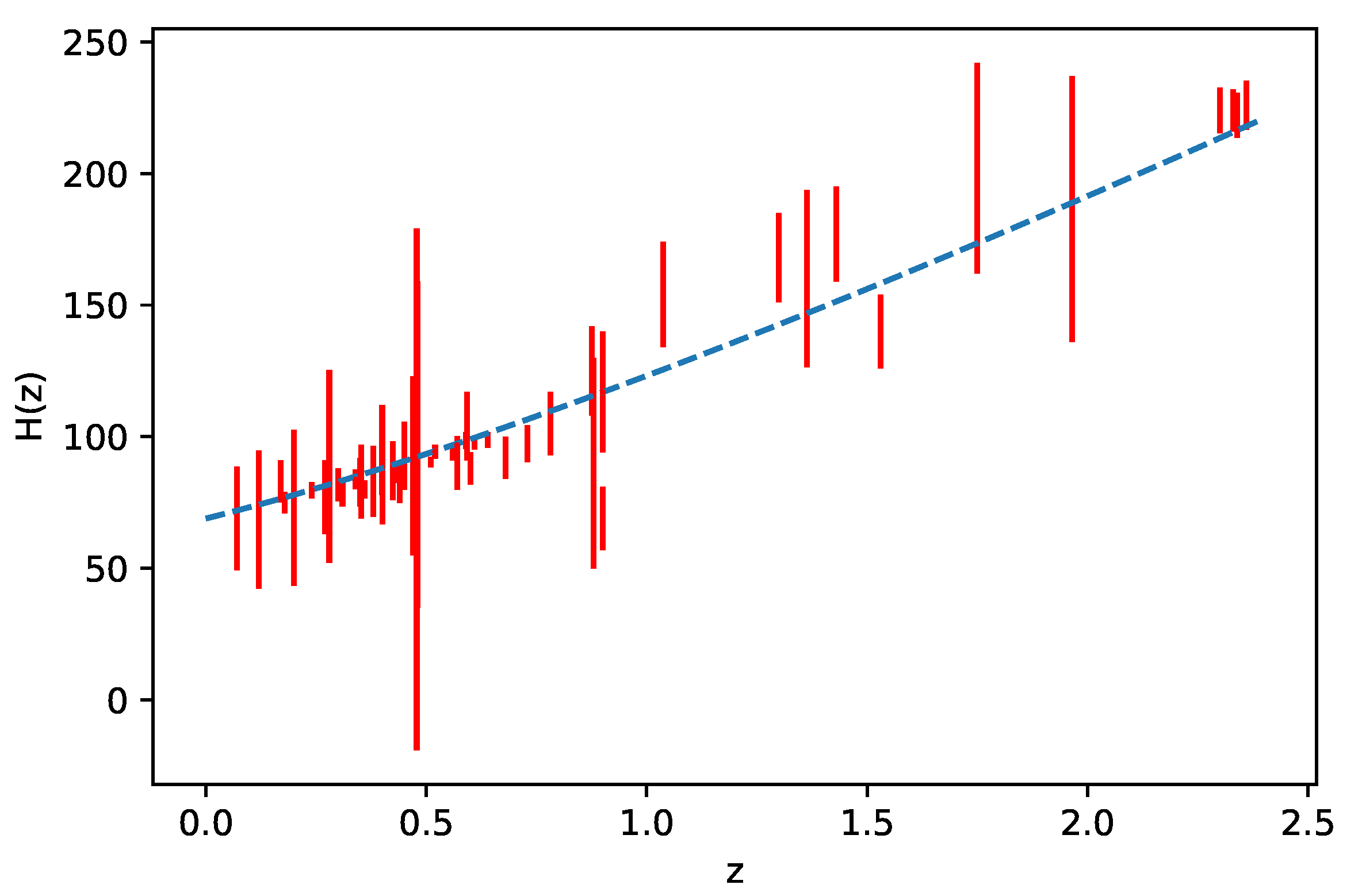
5.1. Cosmic Chronometers Datasets

Finally, in this subsection, we predict the model parameter α and present value of the Hubble parameter H 0 using 57 Hubble data points in the interval of ( 0.07 < z < 2.36 ) , provided by Magana et al. [51].
The related chi-square function is defined as follows to determine the mean value of α and H 0 :
χ H 2 ( α , H 0 ) = i = 1 57 [ H t h ( α , H 0 , z i ) H o b s ( z i ) ] 2 σ i 2 ,
where H t h ( α , H 0 , z i ) and H o b s ( z i ) show the values of the Hubble parameter estimated by the model and measured by the observations, respectively. The measurement of the measured Hubble parameter’s standard error is σ i .

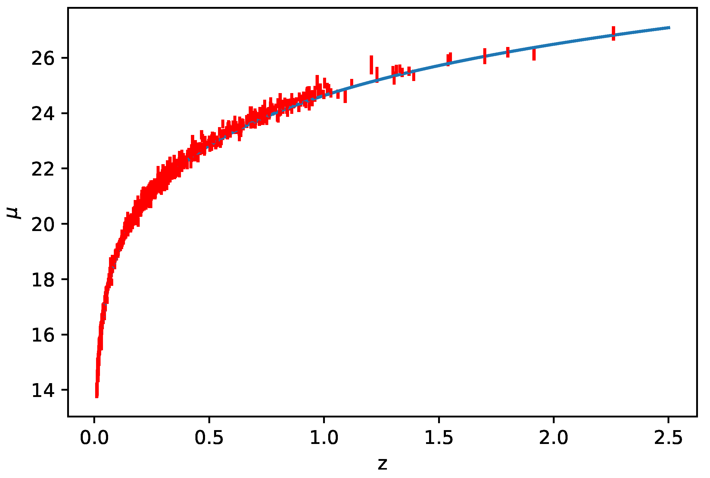
5.2. Pantheon Datasets

In this section, we estimate the parameters α and H 0 using 1048 points from the Pantheon Type 1a supernova dataset (Scolnic et al. [52]). The redshift range of 0.01 < z < 2.3 is supported by 1048 apparent magnitude measurements m B in this dataset.
Distance modulus μ ( z ) in standard cosmology is given by
μ = m B M = 5 l o g 10 ( d l ( z ) ) + 25 ,
where m B is the apparent magnitude, M is the absolute magnitude and, E ( z ) = H ( z ) H 0 being the dimensionless parameter for the expansion rate,
d l ( z ) = c ( 1 + z ) H 0 0 z d z E ( z ) .
is the luminosity distance. Since all supernovae are thought to have the same absolute magnitude, we can use supernova 2002 cr, which has a m B value of 13.907 ± 0.1982 at a low redshift of z = 0.0101 , to calculate absolute magnitude M as described in Goswami et al. [53].
M = 5 l o g 10 H 0 c 1.093 .
We obtain the following equation of apparent magnitude using Equations (25) and (27)
m B = 5 l o g 10 d l ( z ) H 0 c + 23.907 .
The related chi-square function is defined as
χ P a n 2 ( α , H 0 ) = i = 1 1048 [ μ t h ( α , H 0 , z i ) μ o b s ( z i ) ] 2 σ i 2 ,
where μ t h ( α , H 0 , z i ) , μ o b s ( z i ) and σ i 2 are theoretical distance modulus, observational distance modulus and variance at z i , respectively.

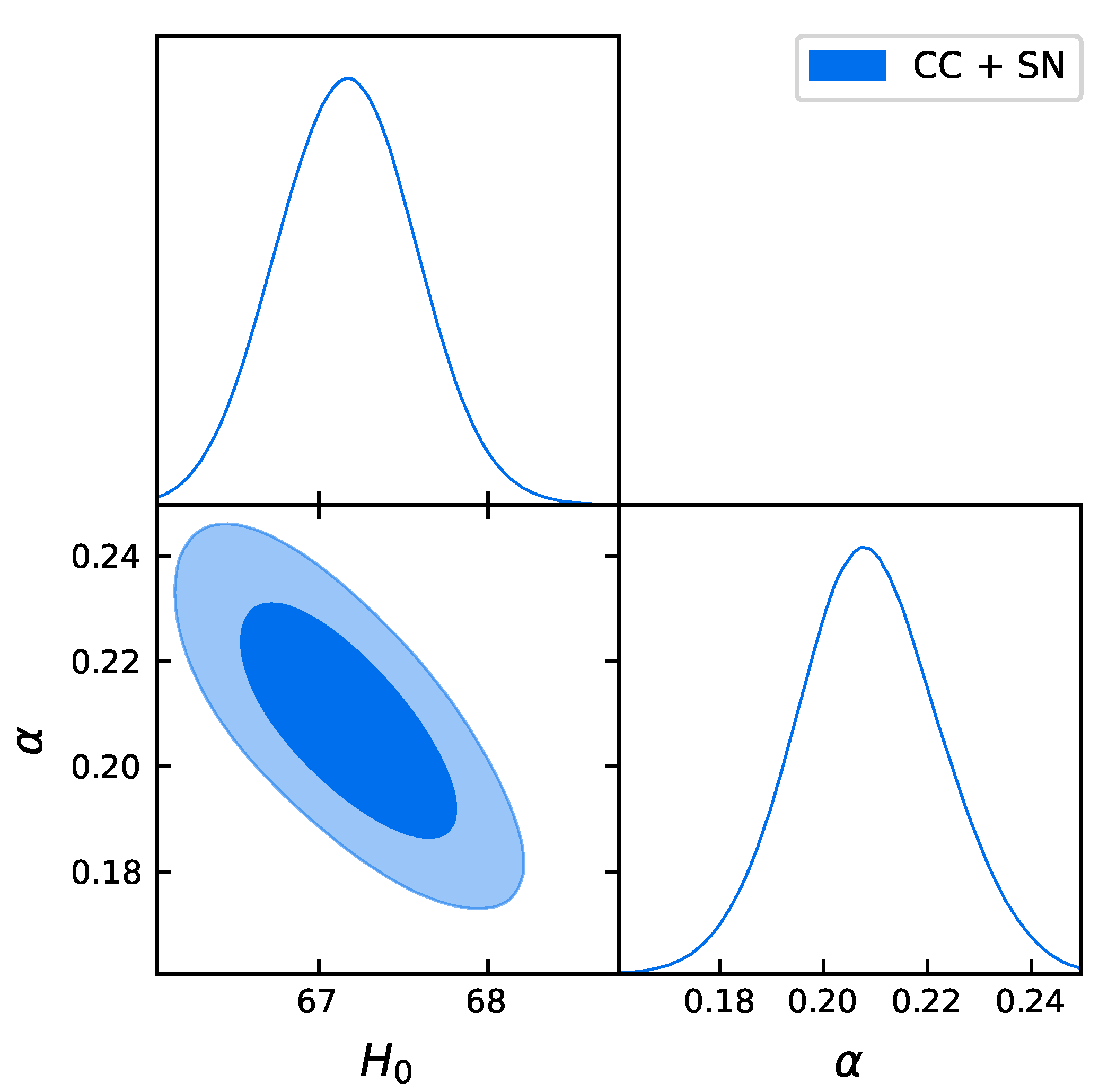
5.3. Observational Result

By minimising the total chi-squared function χ H 2 + χ P a n 2 , we were successful to get the constraints on the parameters of our cosmological model for each of the two separate cases for the combined H(z)+Pantheon datasets. Figure 1 shows the MCMC confidence contours at 1 σ and 2 σ obtained from CC+SN datasets, while Figure 2 and Figure 3 show the curves of H ( z ) and μ ( z ) , respectively. The constrained values of the parameters are summarized in Table 1.

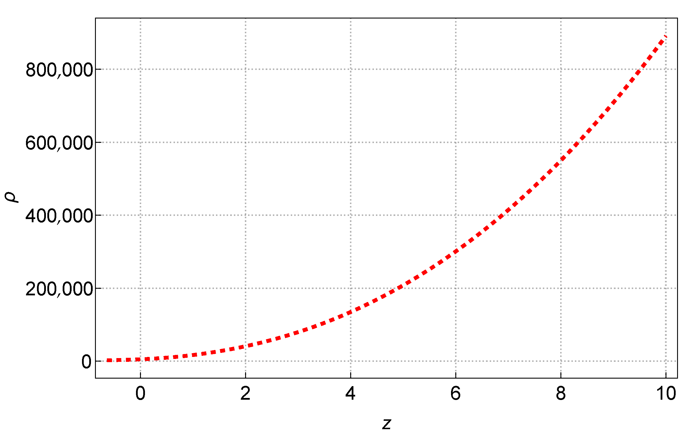
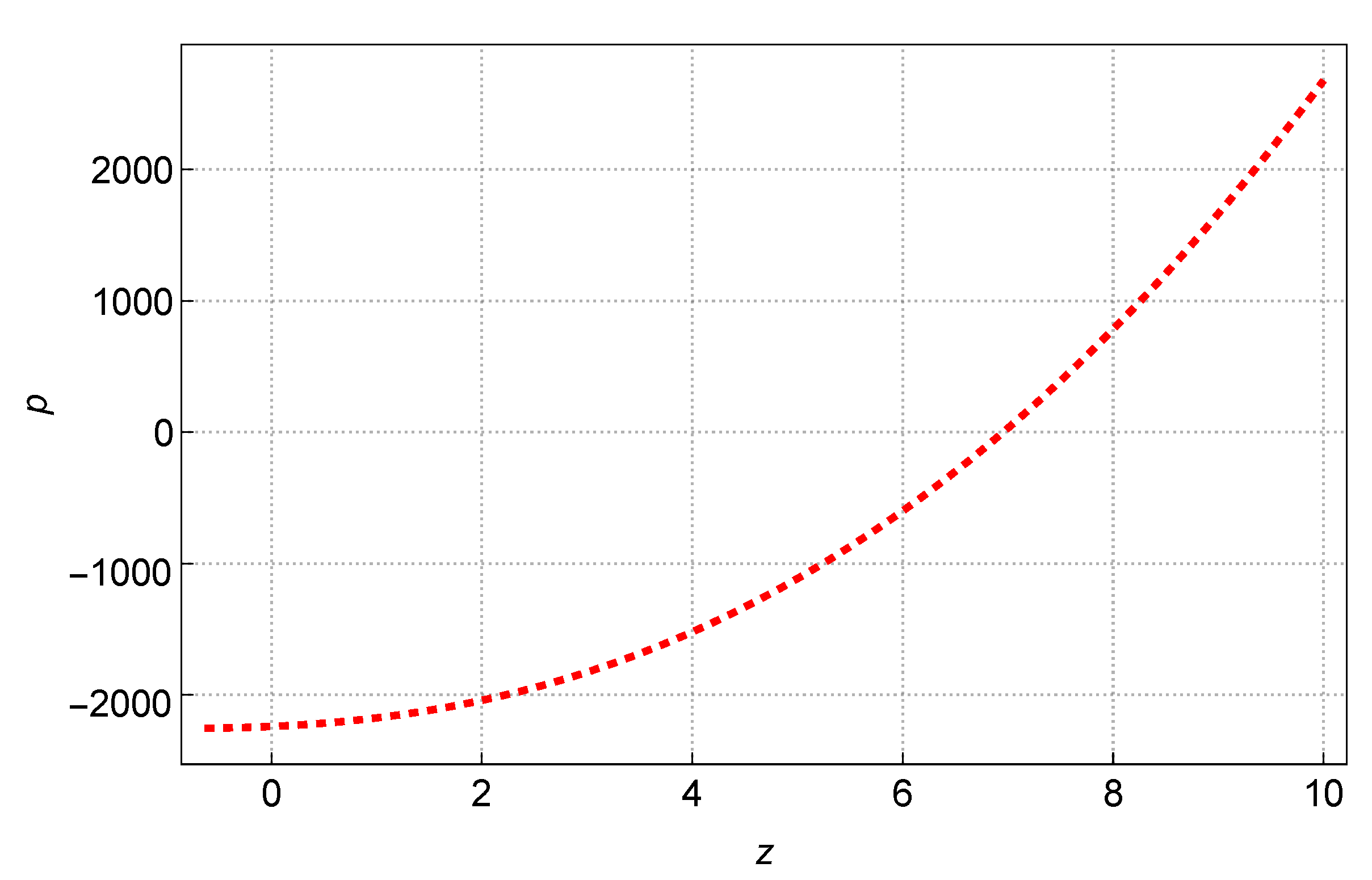
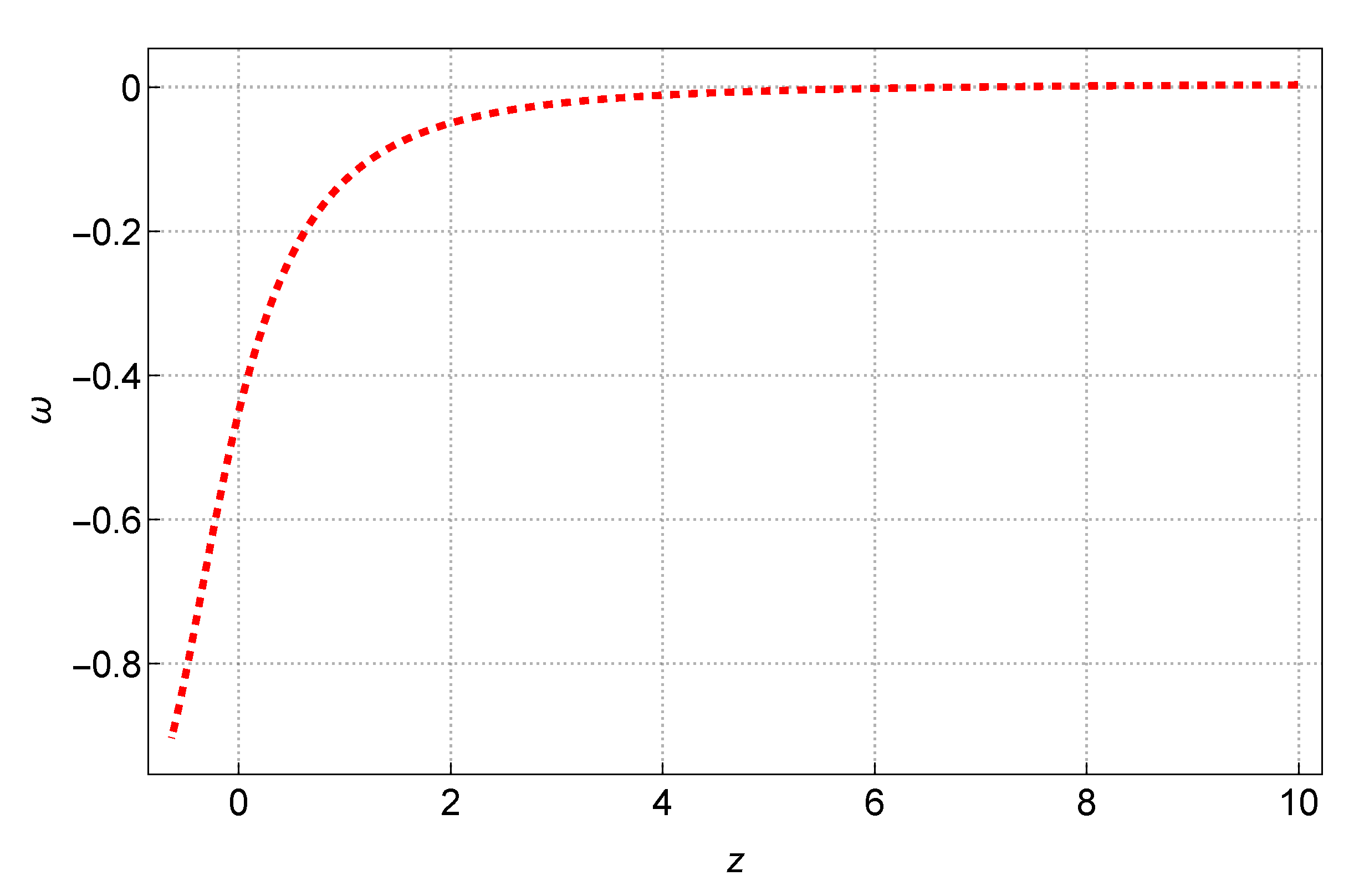
6. Cosmic Pressure, Matter Density and Equation of State Parameter

The expressions of the matter density and cosmic pressure are obtained by using Equation (23)
ρ = 1 [ ( 1 + 3 λ ) 2 λ 2 ] [ ( 3 + 6 λ ) H 0 2 2 [ 1 + ( 1 + z ) 2 ( 1 + α ) ] + 2 λ ( 1 + α ) ( 1 + z ) 2 ( 1 + α ) H 0 2 [ 1 + ( 1 + z ) 2 ( 1 + α ) ] 1 2 ] ,
p = 1 [ ( 1 + 3 λ ) 2 λ 2 ] [ ( 3 + 6 λ ) H 0 2 2 [ 1 + ( 1 + z ) 2 ( 1 + α ) ] 2 ( 1 + 3 λ ) ( 1 + α ) ( 1 + z ) 2 ( 1 + α ) H 0 2 [ 1 + ( 1 + z ) 2 ( 1 + α ) ] 1 2 ] ,
which, on using the equation of state parameter (EoS) ω = p ρ , is calculated as follows
ω = [ ( 3 + 6 λ ) H 0 2 2 [ 1 + ( 1 + z ) 2 ( 1 + α ) ] 2 ( 1 + 3 λ ) ( 1 + α ) ( 1 + z ) 2 ( 1 + α ) H 0 2 [ 1 + ( 1 + z ) 2 ( 1 + α ) ] 1 2 ] [ ( 3 + 6 λ ) H 0 2 2 [ 1 + ( 1 + z ) 2 ( 1 + α ) ] + 2 λ ( 1 + α ) ( 1 + z ) 2 ( 1 + α ) H 0 2 [ 1 + ( 1 + z ) 2 ( 1 + α ) ] 1 2 ] .
We choose λ = 0.5 when representing the behavior of the pressure and energy density. For our model, the energy density has a positive value for all redshift as seen in Figure 4. The density in the model has a decreasing function graph. Comparably, as shown in Figure 5, pressure has positive values at the beginning, and it takes negative values after a certain redshift. Focusing on graphics, it can be seen that the energy density and pressure diverge in the early era and converge to a small positive and negative value, respectively, in the late era.
In Figure 6, the equation of the state parameter evolution trajectory is illustrated. The cosmological constant ( ω = 1 ) , quintessence ( 1 < ω < 1 / 3 ) , or phantom era ( ω < 1 ) are three phases that the accelerating universe could be in. Figure 6 makes it very evident that 1 < ω < 1 3 at the lower redshift era and depicts a fundamental DE quintessence, which denotes an accelerating phase.

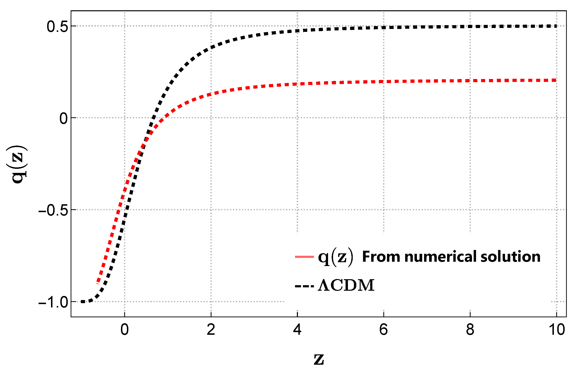
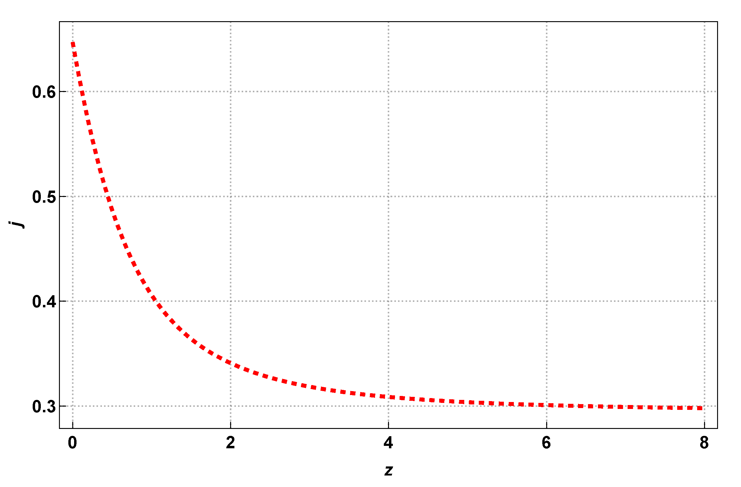
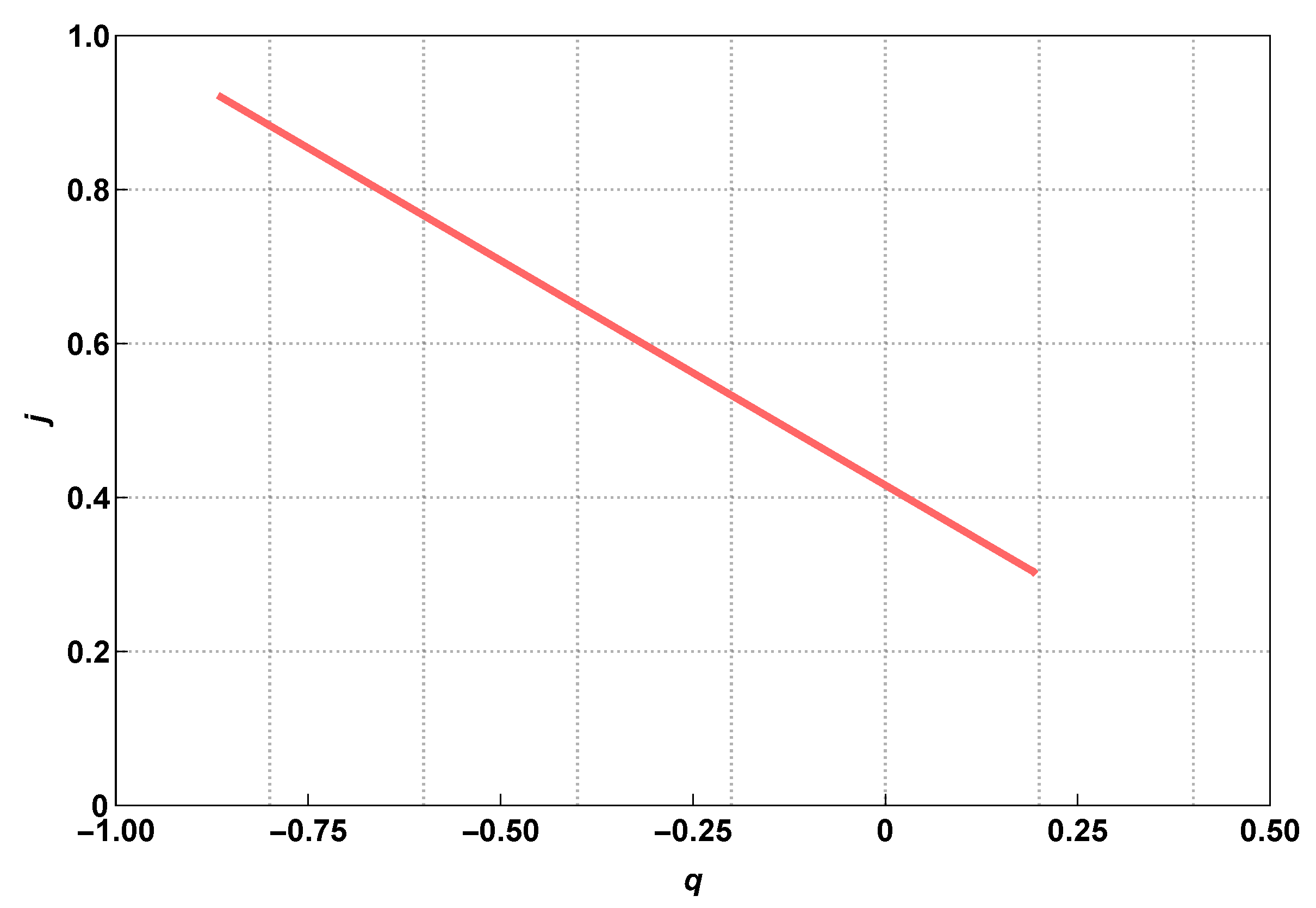
7. Cosmographic Analysis

In this section, we utilize a method known as “cosmography” to discuss the evolution of the universe. It is based on the cosmological principle, which states that on large scales, the observable cosmos is homogeneous and isotropic. Other than the cosmological principle, this study allows us to investigate the evolution of the universe without making any assumptions about specific cosmological models. The method uses Taylor series expansion of the scale factor about t = t 0
a ( t ) a ( t 0 ) = 1 + H 0 ( t t 0 ) q 0 H 0 2 ( t t 0 ) 2 2 ! + j 0 H 0 3 ( t t 0 ) 3 3 ! ,
where subscript 0 denotes the present value of the corresponding parameter.
One defines the Hubble parameter, deceleration parameter and jerk parameter in terms of redshift as
H ( z ) = ( 1 + z ) 1 d z d t ,
q ( z ) = 1 + ( 1 + z ) d H d z H 2 .
j ( z ) = ( 1 + z ) d q d z + q ( 1 + 2 q ) .
We obtained the following value of the jerk parameter of our model in terms of z:
j ( z ) = 2 ( 1 + α ) 2 ( 1 + z ) 2 ( 1 + α ) [ 1 + ( 1 + z ) 2 ( 1 + α ) ] 2 + α ( 1 + α ) [ 1 + ( 1 + z ) 2 ( 1 + α ) ] + 2 α ( 1 + α ) [ 1 + ( 1 + z ) 2 ( 1 + α ) ] 2 .
This fits the standard Λ CDM model’s observations well enough. Figure 7, Figure 8 and Figure 9 show the behavior of the deceleration and jerk parameters, respectively, and also illustrate the nature of these parameters.

8. Conclusions

In the present study, we examined cosmological models in the framework of f ( R , T ) modified theory of gravity on the background of the flat-FRW metric. By adopting the form of f ( R , T ) = R + 2 f ( T ) , we obtained the field equations of this theory. We chose a deceleration parameter that may yield the phase change in the expansion of the universe to satisfy the modified field equations. Then, we analyzed the physical nature of cosmological quantities such as the density, pressure, EoS parameter, and cosmographic parameters corresponding to the constrained values of the model parameters. We estimated the best fit values of model parameters at 1 σ and 2 σ confidence levels by applying the Bayesian analysis and likelihood function together with the MCMC method as seen in Figure 1. in order to be compatible with the recent observational datasets. We used 57 points of the CC datasets, and 1048 points from the Pantheon supernovae samples dataset.
In Figure 2 we plotted the behavior of the Hubble parameter H ( z ) vs. z of our theoretical model and Λ CDM model, respectively, with error bars obtained from the CC and SN data using the MCMC results given in Table 1. The best fit value of H 0 is approximately equal to 67.166 kms 1 Mpc 1 . In Figure 3, we plotted distance modulus μ ( z ) vs. z. The red dotted line with data error bars shows the observed distance modulus, whereas the blue line represents the calculated distance modulus of the generated model. It can be shown that our model is quite consistent with datasets, especially at the lower redshift zone.
We see that the density of energy always takes positive values as shown in Figure 4. The energy density takes high values at high redshift regions, while it approaches zero in low redshift regions. As shown in Figure 5, pressure has positive values at the beginning, and it takes negative values after a certain point of redshift. EoS parameter ω is validated with current values between 1 and 1 / 3 for our model indicating that the DE models are in quintessence phase, which would be the reason of the accelerating expansion, as seen in Figure 6. The evolution of the deceleration parameter q ( z ) in z indicates that our model successfully achieves the late time accelerating expansion together with the decelerating expansion in the past as shown in Figure 7. Figure 7 also displays that the change from decelerating to accelerating expansion phase arose at the redshift z t = 0.844 0.0025 + 0.0027 . The z t values of redshift are representative of the phase transition that occurs in the evolution of the expansion of the universe. Therefore, the model can explain the early decelerating expansion and also the late accelerating expansion. Moreover, it can be seen that the regions where our model has the best fit with the Λ CDM are the low redshift regions. It is observed from Figure 8 and Figure 9 that our model approaches the Λ CDM model ( j = 1 ) as z goes to zero.
Consequently, our f ( R , T ) cosmological model can explain the late time cosmic acceleration without the need of the help of any dark energy component in the matter part of the field equations, by passing from the decelerating phase to the accelerating phase of the universe.

Author Contributions

Conceptualization, R.K.T. and D.S. methodology, B.K.S.; software, B.K.S.; validation, R.K.T., B.K.S., D.S. and D.K.; formal analysis, R.K.T. and D.S.; investigation, R.K.T., B.K.S., D.S. and D.K.; resources, B.K.S. and D.K.; data curation, R.K.T.; writing—original draft preparation, B.K.S., D.S. and D. K; writing—review and editing, B.K.S. and D.S.; visualization, B.K.S.; supervision, R.K.T. and D.S. All authors have read and agreed to the published version of the manuscript.

Funding

This research received no external funding.

Institutional Review Board Statement

Not applicable.

Informed Consent Statement

Not applicable.

Data Availability Statement

Not applicable.

Conflicts of Interest

The authors declare no conflict of interest.

Abbreviations

The following abbreviations are used in this manuscript:
CCCosmic Chronometers
MCMCMarkov Chain Monte Carlo
FRWFriedmann-Robertson-Walker
BAOBaryon acoustic oscillation
BOSSBaryon Oscillation Spectroscopy Survey
ACTPolAtacama Cosmology Telescope Polarimeters
DEDark Energy
EHEinstein-Hilbert
Λ CDM Λ cold dark matter
LRSLocally rotationally symmetric

References

  1. Perlmutter, S.; Gabi, S.; Goldhaber, G.; Goobar, A.; Groom, D.E.; Hook, I.M.; Kim, A.G.; Kim, M.Y.; Lee, J.C.; Pain, R.; et al. Measurements* of the Cosmological Parameters Ω and Λ from the First Seven Supernovae at z ≥ 0.35. Astrophys. J. 1997, 483, 565. [Google Scholar] [CrossRef] [Green Version]
  2. Riess, A.G.; Strolger, L.G.; Casertano, S.; Ferguson, H.C.; Mobasher, B.; Gold, B.; Challis, P.J.; Filippenko, A.V.; Jha, S.; Li, W.; et al. New Hubble space telescope discoveries of type Ia supernovae at z ≥ 1: Narrowing constraints on the early behavior of dark energy. Astrophys. J. 2007, 659, 98. [Google Scholar] [CrossRef] [Green Version]
  3. Spergel, D.N.; Verde, L.; Peiris, H.V.; Komatsu, E.; Nolta, M.R.; Bennett, C.L.; Halpern, M.; Hinshaw, G.; Jarosik, N.; Kogut, A.; et al. First-year Wilkinson Microwave Anisotropy Probe (WMAP)* observations: Determination of cosmological parameters. Astrophys. J. Suppl. Ser. 2003, 148, 175. [Google Scholar] [CrossRef] [Green Version]
  4. Hawkins, E.; Maddox, S.; Cole, S.; Lahav, O.; Madgwick, D.S.; Norberg, P.; Peacock, J.A.; Baldry, I.K.; Baugh, C.M.; Bland-Hawthorn, J.; et al. The 2dF Galaxy Redshift Survey: Correlation functions, peculiar velocities and the matter density of the Universe. Mon. Not. R. Astron. Soc. 2003, 346, 78–96. [Google Scholar] [CrossRef]
  5. Eisenstein, D.J.; Zehavi, I.; Hogg, D.W.; Scoccimarro, R.; Blanton, M.R.; Nichol, R.C.; Scranton, R.; Seo, H.J.; Tegmark, M.; Zheng, Z.; et al. Detection of the baryon acoustic peak in the large-scale correlation function of SDSS luminous red galaxies. Astrophys. J. 2005, 633, 560. [Google Scholar] [CrossRef]
  6. Jain, B.; Taylor, A. Cross-correlation tomography: Measuring dark energy evolution with weak lensing. Phys. Rev. Lett. 2003, 91, 141302. [Google Scholar] [CrossRef] [PubMed] [Green Version]
  7. Ade, P.A.; Aghanim, N.; Arnaud, M.; Ashdown, M.; Aumont, J.; Baccigalupi, C.; Banday, A.J.; Barreiro, R.B.; Bartlett, J.G.; Bartolo, N.; et al. Planck 2015 results-XIII: Cosmological parameters. Astron. Astrophys. 2016, 594, A13. [Google Scholar]
  8. Alam, S.; Ata, M.; Bailey, S.; Beutler, F.; Bizyaev, D.; Blazek, J.A.; Bolton, A.S.; Brownstein, J.R.; Burden, A.; Chuang, C.H.; et al. The clustering of galaxies in the completed SDSS-III Baryon Oscillation Spectroscopic Survey: Cosmological analysis of the DR12 galaxy sample. arXiv 2017, arXiv:1607.03155. [Google Scholar] [CrossRef] [Green Version]
  9. Naess, S.; Hasselfield, M.; McMahon, J.; Niemack, M.D.; Addison, G.E.; Ade, P.A.; Allison, R.; Amiri, M.; Battaglia, N.; Beall, J.A.; et al. The Atacama cosmology telescope: CMB polarization at 200 < < 9000. arXiv 2014, arXiv:1405.5524. [Google Scholar]
  10. Nielsen, J.T.; Guffanti, A.; Sarkar, S. Marginal evidence for cosmic acceleration from Type Ia supernovae. arXiv 2016, arXiv:1506.01354. [Google Scholar] [CrossRef] [Green Version]
  11. Shariff, H.; Jiao, X.; Trotta, R.; Van Dyk, D.A. BAHAMAS: New analysis of type Ia supernovae reveals inconsistencies with standard cosmology. arXiv 2016, arXiv:1510.05954. [Google Scholar] [CrossRef]
  12. Sahni, V. Dark matter and dark energy. arXiv 2004, arXiv:astro-ph/0403324. [Google Scholar]
  13. Padmanabhan, T. Dark energy and gravity. Gen. Relativ. Gravit. 2008, 40, 529–564. [Google Scholar] [CrossRef] [Green Version]
  14. Caldwell, R.R. A phantom menace? Cosmological consequences of a dark energy component with super-negative equation of state. Phys. Lett. B 2002, 545, 23–29. [Google Scholar] [CrossRef] [Green Version]
  15. Sotiriou, T.P.; Faraoni, V. f(R) theories of gravity. Rev. Mod. Phys. 2010, 82, 451. [Google Scholar] [CrossRef] [Green Version]
  16. Harko, T.; Lobo, F.S.N.; Nojiri, S.; Odintsov, S.D. f(R,T) gravity. Phys. Rev. D 2011, 84, 024020. [Google Scholar] [CrossRef] [Green Version]
  17. Sebastiani, L.; Zerbini, S. Static spherically symmetric solutions in F(R) gravity. Eur. Phys. J. C 2011, 71, 1591. [Google Scholar] [CrossRef] [Green Version]
  18. Habib Mazharimousavi, S.; Halilsoy, M.; Tahamtan, T. Solutions for f (R) gravity coupled with electromagnetic field. Eur. Phys. J. C 2012, 72, 1851. [Google Scholar] [CrossRef] [Green Version]
  19. Chakraborty, S.; SenGupta, S. Spherically symmetric brane spacetime with bulk f(R) gravity. Eur. Phys. J. C 2015, 75, 11. [Google Scholar] [CrossRef] [Green Version]
  20. Nojiri, S.; Odintsov, S.D. Unified cosmic history in modified gravity: From F(R) theory to Lorentz non-invariant models. Phys. Rep. 2011, 505, 59. [Google Scholar] [CrossRef] [Green Version]
  21. Myrzakulov, R.; Sebastiani, L.; Vagnozzi, S. Inflation in f(R,ϕ)-theories and mimetic gravity scenario. Eur. Phys. J. C 2015, 75, 444. [Google Scholar] [CrossRef] [Green Version]
  22. Moraes, P.H.R.S. Cosmology from induced matter model applied to 5D f(R,T) theory. Astroph. Space Sci. 2014, 352, 273–279. [Google Scholar] [CrossRef]
  23. Moraes, P.H.R.S. Cosmological solutions from induced matter model applied to 5D gravity and the shrinking of the extra coordinate. Eur. Phys. J. C 2015, 75, 168. [Google Scholar] [CrossRef] [Green Version]
  24. Sharif, M.; Zubair, M.S.M. Thermodynamics in f(R,T) theory of gravity. J. Cosm. Astropart. Phys. 2012, 3, 28. [Google Scholar] [CrossRef] [Green Version]
  25. Moraes, P.H.R.S.; Ribeiro, G.; Correa, R.A.C. A transition from a decelerated to an accelerated phase of the universe expansion from the simplest non-trivial polynomial function of T in the f(R,T) formalism. Astroph. Space Sci. 2016, 361, 227. [Google Scholar] [CrossRef] [Green Version]
  26. Starobinsky, A.A. Disappearing cosmological constant in f(R) gravity. JETP 2007, 86, 157. [Google Scholar] [CrossRef] [Green Version]
  27. Farhoudi, H.S.M. Cosmological and solar system consequences of f(R,T) gravity models. Phys. Rev. D 2014, 90, 044031. [Google Scholar]
  28. Deng, X.M.; Xie, Y. Solar system’s bounds on the extra acceleration of f(R,T) gravity revisited. Int. J. Theor. Phys. 2015, 54, 1739–1749. [Google Scholar] [CrossRef]
  29. Iorio, L. Solar system constraints on a Rindler-type extra-acceleration from modified gravity at large distances. J. Cosmol. Astropart. Phys. 2011, 5, 019. [Google Scholar] [CrossRef] [Green Version]
  30. Fienga, A.; Laskar, J.; Kuchynka, P.; Manche, H.; Desvignes, G.; Gastineau, M.; Cognard, I.; Theureau, G. The INPOP10a planetary ephemeris and its applications in fundamental physics. Celest. Mech. Dyn. Astron. 2011, 111, 363. [Google Scholar] [CrossRef] [Green Version]
  31. Kumar, S. Some FRW models of accelerating universe with dark energy. Astrophys. Space Sci. 2011, 332, 449–454. [Google Scholar] [CrossRef] [Green Version]
  32. Sebastiani, L.; Myrzakulov, R. F(R) gravity and inflation. Int. J. Geom. Meth. Mod. Phys. 2015, 12, 1530003. [Google Scholar] [CrossRef] [Green Version]
  33. Chaubey, R.; Shukla, A.K. A new class of Bianchi cosmological models in f(R,T) gravity. Astrophys. Space Sci. 2013, 343, 415–422. [Google Scholar] [CrossRef]
  34. Adhav, K.S. LRS Bianchi type-I cosmological model in f(R,T) theory of gravity. Astrophys. Space Sci. 2012, 339, 365. [Google Scholar] [CrossRef]
  35. Samanta, G.C. Universe Filled with Dark Energy (DE) from a Wet Dark Fluid (WDF) in f(R,T) Gravity. Int. J. Theor. Phys. 2013, 52, 2303. [Google Scholar] [CrossRef]
  36. Reddy, D.R.K.; Santikumar, R.; Naidu, R.L. Bianchi Type III Cosmological Models in f(R,T) Theory of Gravity. Astrophys. Space Sci. 2012, 342, 249–252. [Google Scholar] [CrossRef]
  37. Reddy, D.R.K.; Naidu, R.L.; Satyanarayana, B. Kaluza-Klein Cosmological Model in f(R,T) Gravity. Int. J. Theor. Phys. 2012, 51, 3222–3227. [Google Scholar] [CrossRef]
  38. Tiwari, R.K.; Sofuoğlu, D. Quadratically varying deceleration parameter in f(R,T) gravity. Int. J. Geom. Meth. Mod. Phys. 2020, 17, 2030003. [Google Scholar] [CrossRef]
  39. Singh, C.P.; Singh, V. Reconstruction of modified f(R,T) gravity with perfect fluid cosmological models. Gen. Rel. Grav. 2014, 46, 1696. [Google Scholar] [CrossRef]
  40. Rao, V.U.M.; Sireesha, K.V.S.; Rao, D.C.P. Perfect fluid cosmological models in a modified theory of gravity. Eur. Phys. J. Plus 2014, 129, 17. [Google Scholar] [CrossRef]
  41. Sharma, N.K.; Singh, J.K. Bianchi Type-II String Cosmological Model with Magnetic Field in f (R, T) Gravity. Int. J. Theor. Phys. 2014, 53, 2912–2922. [Google Scholar] [CrossRef]
  42. Tiwari, R.K.; Sofuoglu, D.; Isik, R.; Shukla, B.K.; Baysazan, E. Non-minimally coupled transit cosmology in f(R,T) gravity. Int. J. Geom. Meth. Mod. Phys. 2022, 19, 2250118. [Google Scholar] [CrossRef]
  43. Tiwari, R.K.; Sofuoglu, D.; Mishra, S.K.; Beesham, A. Anisotropic Model with Constant Jerk Parameter in f(R,T) Gravity. Gravit. Cosmol. 2022, 28, 196–203. [Google Scholar] [CrossRef]
  44. Sahoo, P.K.; Mishra, B.; Reddy, G.C. Axially symmetric cosmological model in f(R,T) gravity. Eur. Phys. J. Plus 2014, 129, 49. [Google Scholar] [CrossRef]
  45. Tiwari, R.K.; Sofuoğlu, D.; Dubey, V.K. Phase transition of LRS Bianchi type-I cosmological model in f(R,T) gravity. Int. J. Geom. Meth. Mod. Phys. 2020, 17, 2050187. [Google Scholar] [CrossRef]
  46. Nagpal, R.; Pacif, S.K.J.; Singh, J.K.; Bamba, K.; Beesham, A. Analysis with observational constraints in Λ-cosmology in f(R,T) gravity. Eur. Phys. J. C 2018, 78, 946. [Google Scholar] [CrossRef] [Green Version]
  47. Debnath, P.S.; Paul, B.C. Observational constraints of emergent universe in f(R,T) gravity with bulk viscosity. Int. J. Geom. Meth. Mod. Phys. 2020, 17, 2050102. [Google Scholar] [CrossRef]
  48. Rudra, P.; Giri, K. Observational constraint in f(R,T) gravity from the cosmic chronometers and some standard distance measurement parameters. Nucl. Phys. B 2021, 967, 115428. [Google Scholar] [CrossRef]
  49. Sardar, G.; Bose, A.; Chakraborty, S. Observational constraints on f(R,T) gravity with f(R,T) = R + h(T). Eur. Phys. J. C 2023, 83, 41. [Google Scholar] [CrossRef]
  50. Sofuoğlu, D.; Tiwari, R.K.; Abebe, A.; Alfedeel, A.H.A.; Hassan, E.I. f(R,T) Gravity and Constant Jerk Parameter in FLRW Spacetime. Physics 2022, 4, 1348–1358. [Google Scholar] [CrossRef]
  51. Magana, J.; Amante, M.H.; Garcia-Aspeitia, M.A.; Motta, V. The Cardassian expansion revisited: Constraints from updated Hubble parameter measurements and type Ia supernova data. Mon. Not. R. Astron. Soc. 2018, 476, 1036–1049. [Google Scholar] [CrossRef]
  52. Scolnic, D.M.; Jones, D.O.; Rest, A.; Pan, Y.C.; Chornock, R.; Foley, R.J.; Huber, M.E.; Kessler, R.; Narayan, G.; Riess, A.G.; et al. The complete light-curve sample of spectroscopically confirmed SNe Ia from Pan-STARRS1 and cosmological constraints from the combined pantheon sample. Astrophys. J. 2018, 859, 101. [Google Scholar] [CrossRef]
  53. Goswami, G.K. Cosmological parameters for spatially flat dust filled Universe in Brans-Dicke theory. Res. Astron. Astrophys. 2017, 17, 27. [Google Scholar] [CrossRef]
Figure 1. MCMC confidence contours at 1 σ and 2 σ obtained from CC+SN datasets.
Symmetry 15 00788 g001
Figure 2. Evolution of H ( z ) vs. z. The theoretical curve of H ( z ) is represented by the blue dashed line while the Λ CDM model is shown as a red dotted line for observed data with the error bars.
Symmetry 15 00788 g002
Figure 3. Evolution of μ ( z ) vs. z. The theoretical curve of μ ( z ) is represented by the blue line while the Λ CDM model is shown as a red dotted line for observed data with the error bars.
Symmetry 15 00788 g003
Figure 4. Evolution of ρ ( z ) vs. z.
Symmetry 15 00788 g004
Figure 5. Evolution of p ( z ) vs. z.
Symmetry 15 00788 g005
Figure 6. Evolution of ω ( z ) vs. z.
Symmetry 15 00788 g006
Figure 7. Evolution of q ( z ) vs. z.
Symmetry 15 00788 g007
Figure 8. Evolution of j ( z ) vs. z.
Symmetry 15 00788 g008
Figure 9. The trajectory of j ( z ) vs. q ( z ) .
Symmetry 15 00788 g009
Table 1. Summary of MCMC results obtained in the article.
DatasetsParameters f ( R , T ) Model
CC α , H 0 0.208573 ± 0.011896 ,
67.166192 ± 0.401849
SN α , H 0 0.208573 ± 0.026998 ,
67.166192 ± 0.7202
Disclaimer/Publisher’s Note: The statements, opinions and data contained in all publications are solely those of the individual author(s) and contributor(s) and not of MDPI and/or the editor(s). MDPI and/or the editor(s) disclaim responsibility for any injury to people or property resulting from any ideas, methods, instructions or products referred to in the content.

