Solution of the Generalized Burgers Equation Using Homotopy Perturbation Method with General Fractional Derivative

Abstract

This research paper introduces the generalized Burgers equation, a mathematical model defined using the general fractional derivative, the most recent operator in fractional calculus. The general fractional derivative can be reduced into three well-known operators, providing a more tractable form of the equation. We apply the homotopy perturbation method (HPM), a powerful analytical technique, to obtain the solution of the generalized Burgers equation. The results are illustrated using a practical example, and we present an analysis of the three reduced operators. In addition, a graphical analysis is provided to visualize the behavior of the solution. This study sheds light on the application of the homotopy perturbation method and the general fractional derivative in solving the generalized Burgers equation, contributing to the field of nonlinear differential equations.

1. Introduction

A logical progression from classical calculus is fractional calculus. Over the past few decades, it has gained popularity and significance across various scientific fields. The growing number of applications for fractional calculus suggests that it gives improved mathematical models for real-world objects. A simulation model is used to sketch the outline of any natural or physical phenomenon that significantly aids in the analysis of the problem. Because of research efforts worldwide, the fractional calculus literature is rapidly expanding. Many areas of the literature have seen the impact of fractional calculus, including biophysics, mechanics, fluid dynamics, heat conduction, sports, control theory, electricity, image processing, viscoelasticity, astrophysics, and electricity ([1,2,3,4,5,6,7,8,9,10,11]). As just a consequence, no aspect of technology or research is unaffected by the calculus of fractional order.

In the study of the calculus of fractional order, we study the derivatives of real or complex order. Many scientific principles are solved using fractional differential equations that can be linear or nonlinear. Many differential equations involving fractional order do not have exact solutions. As a result, many novel numerical and analytical methods are defined to find the answers to such equations. The homotopy perturbation method is a powerful method for solving nonlinear equations due to its simple methodology and higher convergence speed. The well-known mathematician Mr. He invented this method (see [12,13,14]). The result found in series form quickly converges to its exact solution, which is the main advantage of this method. Most of the time, only a few iterations are necessary to get the most accurate results.

In 1915, Bateman citebat introduced the Burgers equation, which was later analyzed by Burgers citebur. We have the Burgers equation in its classical form

$$\frac{\partial v}{\partial \Im }+av\frac{\partial v}{\partial \wp }=c\frac{{\partial }^{2}v}{\partial {\wp }^2}.$$

(1)

Here a can be any arbitrary constant. For detail analysis of Burger’s equation see ([15,16,17,18,19,20,21,22]).

Fractional Calculus is an appealing dimension of science that deals with arbitrary order integrals and derivatives ([23,24,25,26,27,28,29,30]). In contrast to the standard definitions of derivatives and integrals, there are numerous definitions for fractional integrals and derivatives of order $\mu >0$. Samko, Riemann, Liouville, Weyl, Caputo, Almedia, Kilbas, and many others made significant contributions to fractional calculus with singular kernels theory. Sonine, Prabhakar, Miller–Ross, Mainardi, Mittag–Leffler, Gorenglo, Atangana–Baleanu, Wiman, Yang—Abdel–Cattani, and many others contributed to the research of fractional integrals and derivatives with non-singular kernels. General fractional order derivatives are fractional derivatives and integrals in which the non-singular kernel is a special function, such as the Miller–Ross function, Mittag–Leffler function, Wiman function, Rabotnov function, Kohlrausch–William–Watts function, Prabhakar function, and so on. In complex phenomena, general fractional derivatives are thought to be the best method for explicating rheological and relaxation models. The growth and expansion of fractional calculus have resulted in numerous developments in biochemistry, chemistry, physics, biology, medicine, and many other fields.

In the study I found that the Caputo derivative and the general fractional derivative are two different types of fractional derivatives used in fractional calculus to describe the behavior of non-smooth functions. The Caputo derivative is a type of fractional derivative that is defined as the fractional integral of the derivative of a function of order $\mu$, where $0<\mu <1$. It is a type of derivative that takes into account the initial conditions of a function, and it is used to model processes in which the initial conditions are not known or not important. The general fractional derivative, on the other hand, is a more recent operator in fractional calculus that allows for greater flexibility in modeling non-smooth functions. It is defined as a function of order $\mu$ that can be reduced into three well-known operators, making it easier to work with in practice. Unlike the Caputo derivative, the general fractional derivative does not take into account the initial conditions of a function.

In this article, we will look at a generalized Burgers equation in terms of the generalized fractional derivative

$${}_0^C{\mathrm{D}}_{\Im }^{\mu }vs.+a{v}^m\frac{\partial v}{\partial \wp }=c\frac{{\partial }^{2}v}{\partial {\wp }^2}$$

(2)

with

$$v(\wp ,0)=g(\wp ),\wp \in \Omega$$

(3)

where ${}_0^C{\mathrm{D}}_{\Im }^{\mu }$ denotes the generalized derivative of fractional order with respect to ℑ of the order $\mu \in (0,1]$. $\Xi \in R$ is an opened and bounded domain, $\wp \in \Omega$ is arbitrary. The generalized fractional derivative is a type of derivative operator in fractional calculus that can be defined as the inverse operation of the general fractional integral. General fractional derivative, the most recent operator in fractional calculus. The general fractional derivative can be reduced into three well-known operators, providing a more tractable form of the equation.

We call Equation (2) generalized m-Burgers equation. We apply the well-known homotopy perturbation method (HPM) for solving (2) to acquire an approximate symmetric solution underneath the given condition (3).

The structure of this article is divided into seven sections: In Section 2 we define the required definitions and characteristics of fractional differentiation and integration. In Section 3, we discuss the existence and oneness of the symmetry solution. In Section 4, we discuss the steps of the HPM and applied them to the generalized m-Burgers equation. In Section 5 we discuss the convergence analysis and truncation error. The HPM was demonstrated with a basic example in Section 6. Furthermore, Section 7, we discuss how this paper concludes.

2. Preliminaries

This section contains some preliminary information about the newly defined general fractional operator. The mathematicians provide its left Caputo and Riemann–Liouville derivatives of fractional order, according to [31], written as

$${}_0^C{\mathrm{D}}_{\Im }^{\mu }f(\Im )={\int }_0^{\Im }\dot{f}\left(s\right){\Delta }_{\iota }(\Im -s)ds,$$

(4)

$${}_0{\mathrm{D}}_{\Im }^{\mu }f(\Im )=\frac{d}{d\Im }{\int }_0^{\Im }f\left(s\right){\Delta }_{\iota }(\Im -s)ds,$$

(5)

here $\mu \in (0,1)$ known as the order of derivative, $f:[0,+\infty )\to \mathbb{R}$ is a continuous function of absolutely type with $\dot{f}\in L_{\mathrm{loc}}^1(0,+\infty ),0⩽\Im ⩽T<+\infty$, ${\Delta }_{\iota }$ is known as general kernel function. We have the operator follow the linear condition,

$${}_0^C{\mathrm{D}}_{\Im }^{\mu }(jf(\Im )+kg(\Im ))=j{}_0^C{\mathrm{D}}_{\Im }^{\mu }f(\Im )+k{}_0^C{\mathrm{D}}_{\Im }^{\mu }g(\Im ),$$

(6)

$${}_0{\mathrm{D}}_{\Im }^{\mu }(jf(\Im )+kg(\Im ))=j_0{\mathrm{D}}_{\Im }^{\mu }f(\Im )+k_0{\mathrm{D}}_{\Im }^{\mu }g(\Im ).$$

(7)

It is clear that with some restrictions of kernel ${\Delta }_{\iota }(\Im )$, entirely function of monotone type ${\nabla }_{\iota }(\Im )$ exist, for every $\Im >0$ as [31],

$${\Delta }_{\iota }(\Im )*{\nabla }_{\iota }(\Im )={\int }_0^{\infty }{\Delta }_{\iota }\left(s\right){\nabla }_{\iota }(\Im -s)ds=1,$$

(8)

also, for $f\in L_{\mathrm{loc}}^1(0,+\infty )$,we can be write above as

$${}_0{\mathrm{D}}_{\Im }^{-\mu }\left[{}_0^C{\mathrm{D}}_{\Im }^{\mu }f(\Im )\right]=f(\Im )-f\left(0\right),$$

(9)

where ${}_0{\mathrm{D}}_{\Im }^{-\mu }$ shows the general form of Riemann–Liouville integral of fractional order is given by

$${}_0{\mathrm{D}}_{\Im }^{-\mu }f(\Im )={\int }_0^{\Im }f\left(s\right){\nabla }_{\iota }(\Im -s)ds.$$

(10)

We have the right side Caputo as well as Riemann–Liouville derivatives of fractional order are defined as

$${}_{\Im }^C{\mathrm{D}}_T^{\mu }f(\Im )={\int }_{\Im }^T\dot{f}\left(s\right){\Delta }_r(s-\Im )ds,$$

(11)

$${}_{\Im }{\mathrm{D}}_T^{\mu }f(\Im )=\frac{d}{d\Im }{\int }_{\Im }^{T}f\left(s\right){\Delta }_r(s-\Im )ds,$$

(12)

and

$${}_{\Im }{\mathrm{D}}_T^{-\mu }f\left(t\right)={\int }_{\Im }^{T}f\left(s\right){\nabla }_r(s-\Im )ds.$$

(13)

The preceding generalization is coincide with [32], thus, the integration by component formula, based on the results in [32], is satisfied by the aforementioned operators of fractional order as

$${\int }_0^{T}f{\left(s\right)}_0{D}_s^{\mu }g\left(s\right)ds={\int }_0^{T}g{{\left(s\right)}_s}^C{D}_s^{\mu }f\left(s\right)ds,$$

(14)

$${\int }_0^{T}f{\left(s\right)}_0{}^C{D}_s^{\mu }g\left(s\right)ds={\int }_0^{T}g{\left(s\right)}_s{D}_s^{\mu }f\left(s\right)ds.$$

(15)

We have 3 particular cases of a general operator which can be obtained by putting the different kernels in the standard definitions of a general operator. In the first point, if the general kernel is ${\Delta }_{\iota }(\Im )=\frac{t^{-\mu }}{\Gamma (1-\mu )}$; hence, we have the power function ${\nabla }_{\iota }(\Im )=\frac{{\Im }^{\mu -1}}{\Gamma \left(\mu \right)}$ constitutes the integral operator’s associated kernel (10). Consequently, we have from (4) and (5) decrease to Caputo and R-L derivatives, respectively. In our second case we consider the kernel ${\Delta }_{\iota }(\Im )=\frac{\Pi \left(\mu \right)}{1-\mu }{\mathrm{E}}_{\mu }\left(\frac{-\mu }{1-\mu }{\Im }^{\mu }\right)$ in which ${\mathrm{E}}_{\mu }$ and $\mathrm{M}\left(\mu \right)$ are Mittag–Leffler and normalization functions, respectively, with $\mathbf{M}\left(0\right)=\mathbf{M}\left(1\right)=1$. We also have the following relation

$${\nabla }_{\iota }\left(t\right)=\frac{1-\mu }{\Pi \left(\mu \right)}\delta \left(t\right)+\frac{\mu }{\mathrm{M}\left(\mu \right)\Gamma \left(\mu \right)}{t}^{\mu -1}.$$

(16)

Hence, the AB–Caputo as well as AB–Riemann–Liouville derivatives are, respectively, can be obtained by the Equations (4) and (5), and the integral of AB type is [26],

$${}_0{\mathrm{D}}_{\Im }^{-\mu }f(\Im )=\frac{1-\mu }{\mathrm{M}(\wp )}f(\Im )+\frac{\mu }{\mathrm{M}\left(\mu \right)\Gamma \left(\mu \right)}{\int }_0^{\Im }{(\Im -s)}^{\mu -1}f\left(s\right)ds$$

(17)

Furthermore, at the last case, for the CF (Caputo–Fabrizio) derivative ([33,34,35]) is obtained by putting the kernal ${\Delta }_{\iota }(\Im )=\frac{\Pi \left(\mu \right)}{1-\mu }exp\left(\frac{-\mu }{1-\mu }\Im \right)$. Furthermore, $\mathrm{M}\left(\mu \right)$ would be the function used for normalization and it satisfies $M\left(0\right)=M\left(1\right)=1$.

3. Existence and Oneness

In this section, we assume T which is constant as $0<T<\infty ,$ also $(\wp ,\Im )\in \Xi \times (0,T]$. I am going to verify the existence as well as the oneness of the result of the given problem by using the well-known theorem of Banach fixed point. In this concern assume the Branch space of continuous functions which is described on $\Omega \times [0,T]$ ($C(\Omega \times [0,T\left]\right)$) together

$$\parallel v\parallel =\underset{(\wp ,\Im )\in \Omega \times [0,T]}{max}\left|v(\wp ,\Im )\right|.$$

I am going to consider the bellow defined representations for easy handling of the functions.

$$\frac{\partial v}{\partial \wp }=v^{\prime },$$

$$\frac{{\partial }^{2}v}{\partial {\wp }^2}=v^{″},$$

$$f\left(v(\wp ,\Im ),\frac{\partial v(\wp ,\Im )}{\partial \wp },\frac{{\partial }^{2}v(\wp ,\Im )}{\partial {\wp }^2}\right)=-a{v}^m(\wp ,\Im )v^{\prime }(\wp ,\Im )+c{v}^{″}(\wp ,\Im ),$$

(18)

$$:=f(\wp ,\Im ;v(\wp ,\Im )),v^{\prime }(\wp ,\Im ),v^{″}(\wp ,\Im )).$$

Here $f\left(v(\wp ,\Im ),\frac{\partial v(\wp ,\Im )}{\partial \wp },\frac{{\partial }^{2}v(\wp ,\Im )}{\partial {\wp }^2}\right)$ be the functional. $\Xi \in R$ is an opened and bounded domain, $\wp \in \Omega$ is arbitrary. Furthermore, a can be any arbitrary constant.

Lemma 1.

Assume the value of μ lies between 0 and 1, then the following equation satisfies the integral equation

$$\begin{array}{c}\hfill {}_0^C{\mathrm{D}}_{\Im }^{\mu }v(\wp ,\Im )=f(\wp ,\Im ,v(\wp ,\Im )),v^{\prime }(\wp ,\Im ),v^{″}(\wp ,\Im )),\end{array}$$

with

$$\begin{array}{c}\hfill v(\wp ,0)=g(\wp ).\end{array}$$

where $\Xi \in R$ is an opened and bounded domain, $\wp \in \Omega$ is arbitrary. Furthermore, a can be any arbitrary constant.

Proof. 

The proof of the above lemma is straightforward and can be obtained by using the definition of an integral operator. □

Theorem 1.

If $({\theta }_1+{\theta }_2{\chi }_1+{\theta }_3{\chi }_2)\frac{{\Im }^{\mu }}{\Gamma (\mu +1)}<1$, then the function f defined in (18) satisfies the Lipschitz condition.

Proof. 

To find the existence and oneness of the problem, we use the generalized integral operator. Furthermore, these operator reduces in three particular cases for these cases we can separately analysis the existence and oneness of the problem. In that case, first, we consider the first case of the kernel, we get

$$v(\wp ,\Im )=g\left(\wp \right)+\frac{1}{\Gamma \mu }\underset{0}{\overset{\Im }{\int }}{\left(\Im -P\right)}^{\mu -1}f(\wp ,P,v(\wp ,P);v^{\prime }(\wp ,P);v^{″}(\wp ,P))dP.$$

Let $Hu(\wp ,\Im )=v(\wp ,\Im )$, and also prove that H is contraction. By using the theorem named Banach’s fixed point to show that H has a fixed point. It means that it has a unique fixed point.

$$\begin{array}{c}\hfill \begin{array}{c}\left|Hv\right(\wp ,\Im )-Hu(\wp ,\Im \left)\right|\hfill \\ \begin{array}{c}\le \frac{1}{\Gamma \left(\mu \right)}{\int }_0^{\Im }{(\Im -P)}^{\mu -1}\hfill \\ |f(\wp ,P,v(\wp ,p);v^{\prime }(\wp ,P);v^{″}(\wp ,P))-f(\wp ,P,u(\wp ,p);u^{\prime }(\wp ,P);u^{″}(\wp ,P))|dP,\hfill \end{array}\hfill \\ \begin{array}{c}\le \frac{1}{\Gamma \left(\mu \right)}{\int }_0^{\Im }{(\Im -P)}^{\mu -1}\hfill \\ \left({\theta }_1\right|v(\wp ,\Im )-u(\wp ,\Im )|+{\theta }_2|v^{\prime }(\wp ,\Im )-u^{\prime }(\wp ,\Im )|+{\theta }_3|v^{″}(\wp ,\Im )-u^{″}(\wp ,\Im )\left|\right)dP,\hfill \end{array}\hfill \\ \le \frac{({\theta }_1+{\theta }_2{\chi }_1+{\theta }_3{\chi }_2)}{\Gamma \left(\mu \right)}∥u-v∥{\int }_0^{\Im }{(\Im -P)}^{\mu -1}dP,\hfill \\ \le \frac{{\Im }^{\mu }({\theta }_1+{\theta }_2{\chi }_1+{\theta }_3{\chi }_2)}{\Gamma (\mu +1)}∥u-v∥.\hfill \end{array}\end{array}$$

Therefore, using the assumption $({\theta }_1+{\theta }_2{\chi }_1+{\theta }_3{\chi }_2)\frac{{\Im }^{\mu }}{\Gamma (\mu +1)}<1$, we get H is a contraction.

In the other case when our kernel is ${\Delta }_{\iota }(\Im )=\frac{\Pi \left(\mu \right)}{1-\mu }{\mathrm{E}}_{\mu }\left(\frac{-\mu }{1-\mu }{\Im }^{\mu }\right)$ then the generalized operator reduces to the AB type operator. In that case, first, we have the integral equation

$$\begin{array}{c}v(\wp ,\Im )=\frac{1-\mu }{\mathrm{M}(\wp )}f(\wp ,\Im )+\frac{\mu }{\mathrm{M}\left(\mu \right)\Gamma \left(\mu \right)}\hfill \\ \underset{0}{\overset{\Im }{\int }}{\left(\Im -P\right)}^{\mu -1}f(\wp ,P,v(\wp ,P);v^{\prime }(\wp ,P);v^{″}(\wp ,P))dP.\hfill \end{array}$$

Let $Hu(\wp ,\Im )=v(\wp ,\Im )$, and also prove that H is contraction. By using the theorem of Banach’s fixed point to show that H has a fixed point. It means that it has a unique fixed point.

$$\begin{array}{c}\hfill \begin{array}{c}\left|Hv\right(\wp ,\Im )-Hu(\wp ,\Im \left)\right|\hfill \\ \begin{array}{c}\le \frac{\mu }{\mathrm{M}\left(\mu \right)\Gamma \left(\mu \right)}{\int }_0^{\Im }{(\Im -P)}^{\mu -1}\hfill \\ |f(\wp ,P,v(\wp ,P);v^{\prime }(\wp ,P);v^{″}(\wp ,P))-f(\wp ,P,u(\wp ,P);u^{\prime }(\wp ,P);u^{″}(\wp ,P))|dP,\hfill \end{array}\hfill \\ \begin{array}{c}\le \frac{\mu }{\mathrm{M}\left(\mu \right)\Gamma \left(\mu \right)}{\int }_0^{\tau }{(\Im -P)}^{\mu -1}\hfill \\ \left({\theta }_1\right|v(\wp ,\Im )-u(\wp ,\Im )|+{\theta }_2|v^{\prime }(\wp ,\Im )-u^{\prime }(\wp ,\Im )|+{\theta }_3|v^{″}(\wp ,\Im )-u^{″}(\wp ,\Im )\left|\right)dP,\hfill \end{array}\hfill \\ \le \frac{\mu }{\mathrm{M}\left(\mu \right)}\frac{({\theta }_1+{\theta }_2{\chi }_1+{\theta }_3{\chi }_2)}{\Gamma \left(\mu \right)}∥u-v∥{\int }_0^{\tau }{(\Im -p)}^{\mu -1}dP,\hfill \\ \le \frac{{\Im }^{\mu }\mu ({\theta }_1+{\theta }_2{\chi }_1+{\theta }_3{\chi }_2)}{\mathrm{M}\left(\mu \right)\Gamma (\mu +1)}∥u-v∥\hfill \\ \frac{{\Im }^{\mu }\mu ({\theta }_1+{\theta }_2{\chi }_1+{\theta }_3{\chi }_2)}{\mathrm{M}\left(\mu \right)\Gamma (\mu +1)}<1.\hfill \end{array}\end{array}$$

Therefore, using the assumption $\frac{{\Im }^{\mu }\mu ({\theta }_1+{\theta }_2{\chi }_1+{\theta }_3{\chi }_2)}{\mathrm{M}\left(\mu \right)\Gamma (\mu +1)}<1$, we get H is a contraction.

In same the manner, we can obtain the results for CF (Caputo–Fabrizio) operator. □

4. Homotopy Perturbation Method

In solving linear or non-linear problems we see that there are many methods that are given by researchers from time to time. Out of this iteration approach HPM ([36,37]), is a powerful tool for finding the solution to linear or non-linear problems. In this section, we illustrate the HPM. We want to apply the HPM to the given problem (2) and (3). Hence we draw v, as

$$v(\wp ,\Im ;p):\Xi \times [0,T]\times [0,1]\to \mathbb{R}$$

such that

$$\begin{array}{c}H\left(v(\wp ,\Im ;p),p\right)=(1-p)\left[{}_0^C{D}_{\Im }^{\mu }v(\wp ,\Im ;p){-}_0^C{D}_{\Im }^{\mu }{u}_0(\wp ,\Im )\right]\hfill \\ +p\left[{}_0^C{D}_{\Im }^{\mu }v(\wp ,\Im ;p)+a{v}^m(\mu ,\Im ;p)\frac{\partial v(\wp ,\Im ;p)}{\partial \wp }-c\frac{{\partial }^{2}v(\wp ,\Im ;p)}{\partial {\wp }^2}\right]=0,\hfill \end{array}$$

(19)

here p represents an embedding parameter as well as $u_0(\wp ,\Im )$ represents an initial estimation. Now, utilizing the previous equation, (19), we get

$$\begin{array}{c}{}_0^C{D}_{\Im }^{\mu }v(\wp ,\Im ;p){=}_0^C{D}_{\Im }^{\mu }{u}_0(\wp ,\Im )\hfill \\ -p\left[{}_0^C{D}_{\Im }^{\mu }{u}_0(\wp ,\Im )+a{v}^m(\wp ,\Im ;p)\frac{\partial v(\wp ,\Im ;p)}{\partial \wp }-c\frac{{\partial }^{2}v(\wp ,\Im ;p)}{\partial {\wp }^2}\right].\hfill \end{array}$$

(20)

Now, putting $v(\wp ,\Im ;p)={\sum }_{l=0}^{\infty }{p}^l{v}_l(\wp ,\Im )$ in Equation (20), we get

$$\begin{array}{c}{}_0^C{D}_{\Im }^{\mu }{\displaystyle {\displaystyle \sum _{k=0}^{\infty }}}{p}^k{v}_k(\wp ,\Im ){=}_0^C{D}_{\Im }^{\mu }{u}_0(\wp ,\Im )-p\left[D_{\Im }^{\mu }{u}_0(\wp ,\Im )+a{\left({\displaystyle \sum _{k=0}^{\infty }}{p}^k{v}_k(\wp ,\Im )\right)}^m\right.\hfill \\ .\left.\frac{\partial }{\partial \wp }\left({\displaystyle \sum _{k=0}^{\infty }}{p}^k{v}_k(\wp ,\Im )\right)-c\frac{{\partial }^2}{\partial {\wp }^2}\left({\displaystyle \sum _{k=0}^{\infty }}{p}^k{v}_k(\wp ,\Im )\right)\right].\hfill \end{array}$$

(21)

Now, by trying to compare the coefficient values of the respective powers of p in Equation (21), we get:

$$p^0{:}_0^C{D}_{\Im }^{\mu }{v}_0(\wp ,\Im ){=}_0^C{D}_{\Im }^{\mu }{u}_0(\wp ,\Im ),$$

$$\begin{array}{c}\hfill p^1{:}_0^C{D}_{\Im }^{\mu }{v}_1(\wp ,\Im )=-\left({}_0^C{D}_{\Im }^{\mu }{u}_0(\wp ,\Im )+a{v}_0^m(\wp ,\Im )\frac{\partial v_0(\wp ,\Im )}{\partial \wp }\right)+c\frac{{\partial }^2{v}_0(\wp ,\Im )}{\partial {\wp }^2},\end{array}$$

$$\begin{array}{c}\hfill \begin{array}{c}{p}^2{:}_0^C{D}_{\Im }^{\mu }{v}_2(\wp ,\Im )=-a\left[v_0^m(\wp ,\Im )\frac{\partial v_1(\wp ,\Im )}{\partial \wp }+\left.m{v}_0^{m-1}(\wp ,\Im )v_1(\wp ,\Im )\frac{\partial v_0(\wp ,\Im )}{\partial \wp }\right]\right.\hfill \\ +c\frac{{\partial }^2{v}_1(\wp ,\Im )}{\partial {\mu }^2},\hfill \\ ⋮\end{array}\end{array}$$

On taking the generalized integral of fractional type, we get

$$\begin{array}{c}{v}_0(\wp ,\Im )=I_{\Im }^{\mu }\left({}_0^C{D}_{\Im }^{\mu }{u}_0(\wp ,\Im )\right),\hfill \\ v_0(\wp ,\Im )=u_0(\wp ,\Im ),v_0(\wp ,0)=g(\wp ).\hfill \end{array}$$

(22)

$$\begin{array}{c}{v}_1(\wp ,\Im )=-I_{\Im }^{\mu }\left[\left({}_0^C{D}_{\Im }^{\mu }{u}_0(\wp ,\Im )+a{v}_0^m(\wp ,\Im )\frac{\partial v_0(\wp ,\Im )}{\partial \wp }\right)\right.-\hfill \\ \left.c\frac{{\partial }^2{v}_0(\wp ,\Im )}{\partial {\wp }^2}\right],v_1(\wp ,0)=0.\hfill \end{array}$$

$$\begin{array}{c}{v}_2\left(\wp ,\Im \right)=-I_{\Im }^{\mu }\left(a\left[v_0^m(\wp ,\Im )\right.\right.\frac{\partial v_1(\wp ,\Im )}{\partial \wp }+\hfill \\ \left.m{v}_0^{m-1}(\wp ,\Im )v_1(\wp ,\Im )\frac{\partial v_0(\wp ,\Im )}{\partial \wp }\right]+\left.c\frac{{\partial }^2{v}_1(\wp ,\Im )}{\partial {\wp }^2}\right),\hfill \\ ⋮\end{array}$$

(23)

After found these values we can get the result v by putting these values in the following power series.

$$v=v_0+p{v}_1+p^2{v}_2+p^3{v}_3+...$$

(24)

In obtaining results, if we add the limit $p\to 1$ in $v(\wp ,\Im ;p)$, we get the $v(\wp ,\Im )$ of (2) and (3).

5. Analysis of Convergence

In this section, we will study the convergence of the result obtained, which is obtained by HPM for the generalized m-Burgers equation.

Theorem 2.

Let $v_n(\wp ,\Im )$ and $u(\wp ,\Im )$ be the function in the Banach space $C(\Omega \times [0,T\left]\right)$ that is defined in Equation (24). Let us consider that there exists a ℘ that lies between 0 and 1 as $v_n(\wp ,\Im )\le \wp v_{n-1}(\wp ,\Im )$∀$n\in \mathbb{N}$. So we have the series ${\sum }_{l=0}^{\infty }{v}_l(\wp ,\Im )$ converges to $u(\wp ,\Im )$ of the given equation.

Proof. 

Let us consider the partial sum of series ${\sum }_{l=0}^{\infty }{v}_l(\wp ,\Im )$ be $U_n$. Now first we show $U_n$ be a Cauchy sequence in the Branch space $C(\Omega \times [0,T\left]\right)$.

Hence

$$\begin{array}{c}\hfill \begin{array}{c}\left|U_q(\wp ,\Im )-U_r(\wp ,\Im )\right|=\hfill \\ \left|(U_q(\wp ,\Im )-U_{q-1}(\wp ,\Im ))+(U_{q-1}(\wp ,\Im )-U_{q-2}(\wp ,\Im ))+\dots +(U_{r+1}(\wp ,\Im )-U_r(\wp ,\Im ))\right|\hfill \\ \le \left|{\wp }^q{v}_0(\wp ,\Im )+{\wp }^{q-1}{v}_0(\wp ,\Im )+\dots +{\wp }^{r+1}{v}_0(\wp ,\Im )\right|={\wp }^{r+1}(1+\wp +{\wp }^2+\dots +{\wp }^{q-r-1})\left|v_0(\wp ,\Im )\right|\hfill \\ ={\wp }^{r+1}\frac{\left(1-{\wp }^{\left(q-r\right)}\right)}{\left(1-\wp \right)}\left|v_0(\wp ,\Im )\right|,\hfill \end{array}\end{array}$$

Since ℘ lies between 0 and 1 hence

$$∥U_q(\wp ,\Im )-U_r(\wp ,\Im )∥\le \frac{{\wp }^{r+1}}{(1-\wp )}\underset{(\wp ,\Im )\in \Xi \times [0,T]}{max}\left|v_0(\wp ,\Im )\right|.$$

(25)

Furthermore, since $v_0$ is bounded,

$$\underset{q,r\to \infty }{lim}∥U_q(\wp ,\Im )-U_r(\wp ,\Im )∥=0.$$

Thus, by definition of the Cauchy sequence, we reached the desired result. □

Theorem 3.

Show that the maximal absolute truncation error for the series solution $v(\wp ,\Im )={\sum }_{l=0}^{\infty }{v}_l(\wp ,\Im )$ of the given problem by

$$\left|v(\wp ,\Im )-\sum _{i=0}^r{v}_i(\wp ,\Im )\right|\le \frac{{\wp }^{r+1}}{(1-\wp )}∥v_0∥.$$

Proof. 

To prove the theorem we tack the limit as $q\to \infty$ in Equation (25), we obtain

$$\begin{array}{c}\hfill \left|v(\wp ,\Im )-S_r\right|\le \frac{{\wp }^{r+1}}{(1-\wp )}\underset{(\wp ,\Im )\in \Xi \times [0,T]}{max}\left|v_0(\wp ,\Im )\right|.\end{array}$$

Hence, we obtain the desired result

$$\left|v(\wp ,\Im )-\sum _{l=0}^r{v}_l(\wp ,\Im )\right|\le \frac{{\wp }^{r+1}}{(1-\wp )}∥v_0∥.$$

□

6. Examples

The purpose of this section is to utilize a mathematical technique known as the homotopy perturbation method (HPM) that was previously introduced, in order to solve a particular example of the generalized Burgers equation. By employing the HPM, we can easily derive an approximate solution to this specific instance of the generalized Burgers equation, which is represented by Equations (2) with (3).

Example 1.

Consider $(\wp ,\Im )\in (0,1)\times (0,T]$, $\mu \in (0,1]$ and we have the following generalized Burgers equation

$$\begin{array}{c}\hfill {}_0^C{D}_{\Im }^{\mu }v(\wp ,\Im )=-av(\wp ,\Im )\frac{\partial v(\wp ,\Im )}{\partial \wp }+c\frac{{\partial }^{2}v(\wp ,\Im )}{\partial {\wp }^2},\end{array}$$

(26)

with the initial condition

$$v_0=u_0={\wp }^2.$$

(27)

Now by using the homotopy technique, and the the relation defined in Equation (27), we get

$$\begin{array}{c}\hfill \begin{array}{c}{}_0^C{D}_{\Im }^{\mu }v(\wp ,\Im ;p)={}_0^C{D}_{\Im }^{\mu }{u}_0(\wp ,\Im )\hfill \\ -p\left({}_0^C{D}_{\Im }^{\mu }{u}_0(\wp ,\Im )+av(\wp ,\Im ;p)\frac{\partial v(\wp ,\Im ;p)}{\partial \wp }-c\frac{{\partial }^{2}v(\wp ,\Im ;p)}{\partial {\wp }^2}\right).\hfill \end{array}\end{array}$$

(28)

As we have

$$v(\wp ,\Im ;p)=\sum _{l=0}^{\infty }{p}^l{v}_l(\wp ,\Im ).$$

(29)

By putting the value of Equation (29) into Equation (28) and collecting the coefficients of various terms of p, we obtain

$$p^0{:}_0^C{D}_{\Im }^{\mu }{v}_0(\wp ,\Im ){=}_0^C{D}_{\Im }^{\mu }{u}_0(\wp ,\Im ),$$

$$\begin{array}{c}\hfill p^1{:}_0^C{D}_{\Im }^{\mu }{v}_1(\wp ,\Im )=-\left({}_0^C{D}_{\Im }^{\mu }{u}_0(\wp ,\Im )+a{v}_0(\wp ,\Im )\frac{\partial v_0(\wp ,\Im )}{\partial \wp }\right)+c\frac{{\partial }^2{v}_0(\wp ,\Im )}{\partial {\wp }^2},\end{array}$$

$$\begin{array}{c}\hfill \begin{array}{c}{p}^2{:}_0^C{D}_{\Im }^{\mu }{v}_2(\wp ,\Im )=-a\left[v_0(\wp ,\Im )\frac{\partial v_1(\wp ,\Im )}{\partial \wp }+\left.v_1(\wp ,\Im )\frac{\partial v_0(\wp ,\Im )}{\partial \wp }\right]\right.\hfill \\ +c\frac{{\partial }^2{v}_1(\mu ,\Im )}{\partial {\mu }^2},\hfill \end{array}\end{array}$$

$$\begin{array}{c}\hfill \begin{array}{c}{p}^3{:}_0^C{D}_{\Im }^{\mu }{v}_3(\wp ,\Im )=\left\{-a\left[v_0(\wp ,\Im )\frac{\partial v_2(\wp ,\Im )}{\partial \wp }+v_1(\wp ,\Im )\frac{\partial v_1(\wp ,\Im )}{\partial \wp }+\right.\right.\hfill \\ \left.v_2(\wp ,\Im )\frac{\partial v_0(\wp ,\Im )}{\partial \wp }\right]\left.+c\frac{{\partial }^2{v}_2(\mu ,\Im )}{\partial {\mu }^2}\right\},\hfill \end{array}\\ ⋮\end{array}$$

By using ${\mathcal{I}}_{\Im }^{\mu }$ the generalized integral operator, we get

$$p^0:v_0(\wp ,\Im )=u_0(\wp ,\Im ),$$

$$\begin{array}{c}\hfill p^1:v_1(\wp ,\Im )=I_{\Im }^{\mu }\left\{-\left(D_{\Im }^{\mu }{u}_0(\wp ,\Im )+a{v}_0(\wp ,\Im )\frac{\partial v_0(\wp ,\Im )}{\partial \wp }\right)+c\frac{{\partial }^2{v}_0(\wp ,\Im )}{\partial {\wp }^2}\right\},\end{array}$$

$$\begin{array}{c}\hfill p^2:v_2(\wp ,\Im )=I_{\Im }^{\mu }\left\{-a\left(v_0(\wp ,\Im )\frac{\partial v_1(\wp ,\Im )}{\partial \wp }+v_1(\wp ,\Im )\frac{\partial v_0(\wp ,\Im )}{\partial \wp }\right)+c\frac{{\partial }^2{v}_1(\wp ,\Im )}{\partial {\mu }^2}\right\},\end{array}$$

$$\begin{array}{c}\hfill \begin{array}{c}{p}^3:v_3(\wp ,\Im )=I_{\Im }^{\mu }\left\{-a\left[v_0(\wp ,\Im )\frac{\partial v_2(\wp ,\Im )}{\partial \wp }+v_1(\wp ,\Im )\frac{\partial v_1(\wp ,\Im )}{\partial \wp }+\right.\right.\hfill \\ \left.v_2(\wp ,\Im )\frac{\partial v_0(\wp ,\Im )}{\partial \wp }\right]\left.+c\frac{{\partial }^2{v}_2(\mu ,\Im )}{\partial {\mu }^2}\right\},\hfill \end{array}\\ ⋮\end{array}$$

Once these values have been ascertained, the resultant value v may be obtained by substituting them into the power series (24), thus obtaining the desired solution.

Moving forward, we shell delineate all three scenarios for the aforementioned problem.

6.1. Case I

By applying various kernels to the standard definitions of the general operator, we can derive three specific cases of the operator. Out of these three cases, in first case, we consider the general kernel as ${\Delta }_{\iota }(\Im )=\frac{t^{-\mu }}{\Gamma (1-\mu )}$; hence, the associated power function is ${\nabla }_{\iota }(\Im )=\frac{{\Im }^{\mu -1}}{\Gamma \left(\mu \right)}$. It has the ability to effortlessly produce the type I integral operator. As a result, Equation (2) reduces to the type I derivative operator. Hence by using the above-defined approach, we can easily solve the considered example, the steps are defined bellow

$$v_0=u_0={\wp }^2,$$

On using the above relation defined above, we get

$${\displaystyle \frac{\partial }{\partial \wp }}{v}_0(\wp ,\Im )=2\wp$$

also

$$\frac{{\partial }^2}{\partial {\wp }^2}{v}_0(\wp ,\Im )=2,$$

by using the above values, we obtain

$$v_1(\wp ,\Im )=\left(2c-2a{\wp }^3\right)\frac{{\Im }^{\mu }}{\Gamma \left(\mu +1\right)},$$

(30)

now to find the value of $v_2$, we have

$$\begin{array}{c}{v}_2(\wp ,\Im )=2a\wp \left(5a{\wp }^3-8c\right){\left(\frac{{\Im }^{\mu }}{\Gamma \left(\mu +1\right)}\right)}^2,\\ ⋮\end{array}$$

(31)

Hence, the rest terms can be easily obtained and by using relation (24), we can easily find the approximate solution

$$\begin{array}{c}v(\wp ,\Im )={\wp }^2+\left(2c-2a{\wp }^3\right)\frac{{\Im }^{\mu }}{\Gamma \left(\mu +1\right)}\hfill \\ +2a\wp \left(5a{\wp }^3-8c\right){\left(\frac{{\Im }^{\mu }}{\Gamma \left(\mu +1\right)}\right)}^2+...\hfill \end{array}$$

(32)

Now to plot the numerical results for the obtained solution, we consider a = 0.5 and c = 1. We plot three graphs for different values of $\mu$, 0.5, 0.8 and 1, respectively.

6.2. Case II

In the next case, we assume the value of the kernel for the general operator ${\Delta }_{\iota }(\Im )=\frac{\Pi \left(\mu \right)}{1-\mu }exp\left(\frac{-\mu }{1-\mu }\Im \right)$. In that operator $\mathrm{M}\left(\mu \right)$ represents normalization functions. Now we follow the steps defined above and solve the considered example.

$$v_0=u_0={\wp }^2.$$

Now by using the homotopy technique, and the relation defined in Equation (27), we get

$${\displaystyle \frac{\partial }{\partial \wp }}{v}_0(\wp ,\Im )=2\wp$$

and

$$\frac{{\partial }^2}{\partial {\wp }^2}{v}_0(\wp ,\Im )=2,$$

we get

$$v_1(\wp ,\Im )=\left(2-\mu \right)\left(c-a{\wp }^3\right)\left(1-\mu +\frac{{\Im }^{\mu }}{\Gamma \mu }\right).$$

(33)

Next, to find $v_2$, we have

$$\begin{array}{c}{v}_2(\wp ,\Im )=\frac{a\wp {\left(2-\mu \right)}^2}{2}\left(5a{\wp }^3-8c\right){\left(1-\mu +\frac{{\Im }^{\mu }}{\Gamma \mu }\right)}^2,\\ ⋮\end{array}$$

(34)

Hence, by the same approach be can easily find the approximate solution

$$\begin{array}{c}v(\wp ,\Im )={\wp }^2+\left(2-\mu \right)\left(c-a{\wp }^3\right)\left(1-\mu +\frac{{\Im }^{\mu }}{\Gamma \mu }\right)\hfill \\ +\frac{a\wp {\left(2-\mu \right)}^2}{2}\left(5a{\wp }^3-8c\right){\left(1-\mu +\frac{{\Im }^{\mu }}{\Gamma \mu }\right)}^2+...,\hfill \end{array}$$

(35)

Now to plot the numerical results for the obtained solution, we consider a = 0.5 and c = 1. We plot three graphs for different values of $\mu$, 0.5, 0.8 and 1, respectively.

6.3. Case III

In our third case, we assume the value of the kernel for the general operator ${\Delta }_{\iota }(\Im )=\frac{\Pi \left(\mu \right)}{1-\mu }{\mathrm{E}}_{\mu }\left(\frac{-\mu }{1-\mu }{\Im }^{\mu }\right)$. In which ${\mathrm{E}}_{\mu }$ represent Mittag–Leffler function and $\mathrm{M}\left(\mu \right)$ represents normalization functions. Now we follow the steps defined above and solve the considered example. On solving we get

$$v_0=u_0={\wp }^2.$$

Now by using the homotopy technique, and the relation defined in Equation (27), we get

$${\displaystyle \frac{\partial }{\partial \wp }}{v}_0(\wp ,\Im )=2\wp$$

and

$$\frac{{\partial }^2}{\partial {\wp }^2}{v}_0(\wp ,\Im )=2,$$

we obtain

$$v_1(\wp ,\Im )=\frac{4\left(c-a{\wp }^3\right)\left(1-\mu +\mu \Im \right)}{\left(2-\mu \right)M\left(\mu \right)},$$

(36)

on the same way, we can easily find $v_2$, as

$$\begin{array}{c}{v}_2(\wp ,\Im )=\frac{4a\wp \left(5a{\wp }^3-8c\right){\left(1-\mu +\mu \Im \right)}^2}{\left(2-\mu \right)M\left(\mu \right)},\\ ⋮\end{array}$$

(37)

Hence, by the same approach be can easily find the approximate solution

$$\begin{array}{c}v(\wp ,\Im )={\wp }^2+2\left(c-a{\wp }^3\right)\left(1-\mu +\mu \Im \right)+\hfill \\ 2a\wp \left(5a{\wp }^3-8c\right){\left(1-\mu +\mu \Im \right)}^2+...,\hfill \end{array}$$

(38)

Now to plot the numerical results for the solution obtained, we consider a = 0.5 and c = 1. We plot three graphs for different values of $\mu$, 0.5, 0.8 and 1, respectively.

As we have fractional calculus is a powerful branch to deal with mathematical modeling. It provides us with more precise results to describe the physical models (see [38,39,40,41,42,43]). I use a generalized operator which provides us with three particular cases of the well-known fractional operator. I am providing the numerical results for the solution obtained for all cases. In this concern, I consider $a=0.5$ and $c=1$. The plot three graphs for different values of $\mu$, 0.5, 0.8 and 0.9, respectively, at ℑ equal to 1.

7. Conclusions

In this research paper, we considered the generalized Burgers equation with the help of a generalized fractional operator. We use the HPM to find the solution to some standard examples. We find the results of the defied problem and also discuss its three particular results as well. At last, we plot Figure 1, Figure 2, Figure 3, Figure 4, Figure 5, Figure 6, Figure 7, Figure 8, Figure 9, Figure 10, Figure 11 and Figure 12 of that example to show the efficiency of the generalized operator.

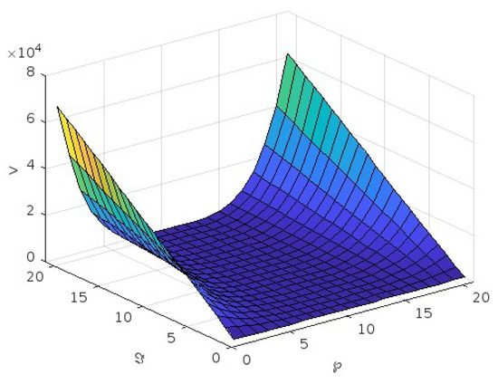
Figure 1. Graph of v for the first case for $\mu =0.5,a=0.5,c=1$.

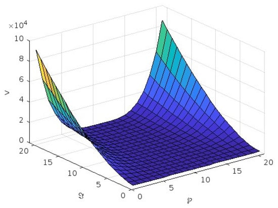
Figure 2. Graph of v for first case for $\mu =0.8,a=0.5,c=1$.

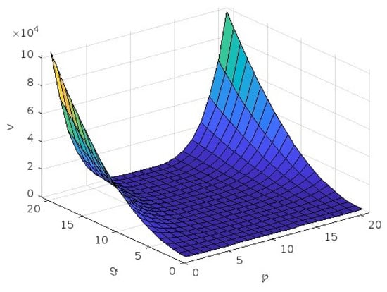
Figure 3. Graph of v for first case for $\mu =1,a=0.5,c=1$.

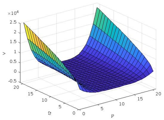
Figure 4. Graph of v for second case for $\mu =0.5,a=0.5,c=1$.

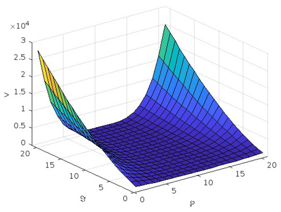
Figure 5. Graph of v for the second case for $\mu =0.8,a=0.5,c=1$.

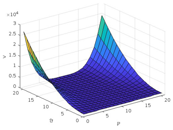
Figure 6. Graph of v for the second case for $\mu =1,a=0.5,c=1$.

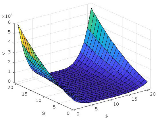
Figure 7. Graph of v for third case for $\mu =0.5,a=0.5,c=1$.

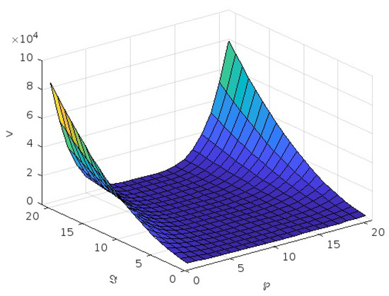
Figure 8. Graph of v for third case for $\mu =0.8,a=0.5,c=1$.

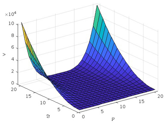
Figure 9. Graph of v for third case for $\mu =1,a=0.5,c=1$.

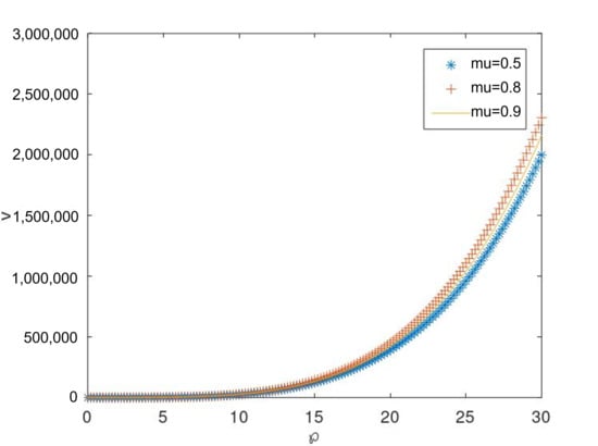
Figure 10. Graph of v for case I, with respect to ℘ for different values of $\mu =0.5,0.8,0.9$, respectively, at a = 0.5, c = 1, $\Im =1$.

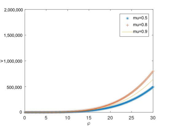
Figure 11. Graph of v for case II, with respect to ℘ for different values of $\mu =0.5,0.8,0.9$, respectively, at a = 0.5, c = 1, $\Im =1$.

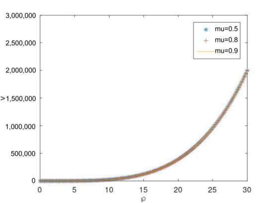
Figure 12. Graph of v for case III, with respect to ℘ for different values of $\mu =0.5,0.8,0.9$, respectively, at a = 0.5, c = 1, $\Im =1$.

References

- Kilbas, A. Fractional Calculus of the Generalized Wright Function; Fractional Calculus and Applied Analysis; Institute of Mathematics and Informatics Bulgarian Academy of Sciences: Sofia, Bulgaria, 2005; Volume 8, pp. 113–126. [Google Scholar]
- Miller, K.S.; Ross, B. An Introdution to the Fractional Calculus and Fractional Differential Equations; J. Willey & Sons: New York, NY, USA, 1993. [Google Scholar]
- Podlubny, I. Fractional Differential Equations; Academic Press: San Diego, CA, USA, 1999. [Google Scholar]
- Sharma, S.; Goswami, P.; Baleanu, D.; Dubey, R.S. Comprehending the model of omicron variant using fractional derivatives. Appl. Math. Sci. Eng. 2023, 31, 2159027. [Google Scholar] [CrossRef]
- Dubey, R.S.; Goswami, P.; Baskonus, H.M.; Gomati Tailor A., G. On the existence and uniqueness analysis of fractional blood glucose-insulin minimal model. Int. J. Model. Simul. Sci. Comput. 2022. [Google Scholar] [CrossRef]
- Chaurasia, V.B.L.; Dubey, R.S. Analytical solution for the generalized time-fractional telegraph equation. Fract. Differ. Calc. 2013, 3, 21–29. [Google Scholar] [CrossRef]
- Jafari, H.; Prasad, J.G.; Goswami, P.; Dubey, R.S. Solution of the local fractional generalized KDV equation using homotopy analysis method. Fractals 2021, 29, 2140014. [Google Scholar] [CrossRef]
- Dubey, R.S.; Goswami, P.; Gill, V. A new analytical method to solve Klein-Gordon equations by using homotopy perturbation Mohand transform method. Malaya J. Mat. 2022, 10, 1–19. [Google Scholar] [CrossRef]
- Kilbas, A.A.; Srivastava, H.M.; Trujillo, J.J. Theory and Applications of Fractional Differential Equations; Elsevier North-Holland Science Publishers: Amsterdam, The Netherlands; London, UK; New York, NY, USA, 2006. [Google Scholar]
- Gao, W.; Yel, G.; Baskonus, H.M.; Cattani, C. Complex Solitons in the Conformable (2+ 1)-dimensional Ablowitz-Kaup-Newell-Segur Equation. AIMS Math. 2020, 5, 507–521. [Google Scholar] [CrossRef]
- Dubey, R.S.; Singh, Y.; Agarwal, P.; Saini, G.L.; Singh, V. Some results on the new fractional derivative of generalized k-Wright function. J. Interdiscip. Math. 2020, 23, 607–615. [Google Scholar] [CrossRef]
- He, J.H. Homotopy perturbation technique. Comput. Methods Appl. Mech. Eng. 1999, 178, 257–262. [Google Scholar] [CrossRef]
- He, J.H. Homotopy perturbation method for solving boundary value problems. Phys. Lett. A 2006, 350, 87–88. [Google Scholar] [CrossRef]
- He, J.H. The homotopy perturbation method for nonlinear oscillators with discontinuities. Appl. Math. Comput. 2004, 151, 287–292. [Google Scholar] [CrossRef]
- Malyk, I.; Shrahili, M.M.A.; Shafay, A.R.; Goswami, P.; Sharma, S.; Dubey, R.S. Analytical solution of non-linear fractional Burger’s equation in the framework of different fractional derivative operators. Results Phys. 2020, 19, 103397. [Google Scholar] [CrossRef]
- Burgers, J.M. A mathematical model illustrating the theory of turbulence. In Advances in Applied Mechanics; Elsevier: Amsterdam, The Netherlands, 1948; Volume 1, pp. 171–199. [Google Scholar]
- Hopf, E. The Partial Differential Equation ut+uux=μuxx. Commun. Pure Appl. Math. 1950, 3, 201–230. [Google Scholar] [CrossRef]
- Yokus, A.; Kaya, D. Numerical and exact solutions for time fractional Burger’s equation. J. Nonlinear Sci. Appl. 2017, 10, 3419–3428. [Google Scholar] [CrossRef]
- Saad, K.M.; Atangana, A.; Baleanu, D. New fractional derivatives with non-singular kernel applied to the Burgers equation. Chaos Interdiscip. J. Nonlinear Sci. 2018, 28, 063109. [Google Scholar] [CrossRef]
- Saad, K.M.; Al-Sharif, E.H.F. Analytical study for time and time-space fractional Burgers’ equation. Adv. Differ. Equ. 2017, 2017, 300. [Google Scholar] [CrossRef]
- Joshi, M.S.; Desai, N.B.; Mehta, M.N. Solution of the Burger’s Equation for Longitudinal Dispersion Phenomena Occurring in Miscible Phase Flow through Porous Media. J. Eng. Technol. Sci. 2012, 44, 12–16. [Google Scholar] [CrossRef]
- Kilicman, A.; Shokhanda, R.; Goswami, P. On the solution of (n + 1)-dimensional fractional M-Burgers equation Authors. Alex. Eng. J. 2021, 60, 1165–1172. [Google Scholar] [CrossRef]
- Yel, G.; Cattani, C.; Baskonus, H.M.; Gao, W. On the Complex Simulations with Dark-Bright to the Hirota-Maccari System. J. Comput. Nonlinear Dyn. 2021, 16, 061005. [Google Scholar] [CrossRef]
- Liu, J.G.; Yang, X.J.; Feng, Y.Y.; Cui, P. New fractional derivative with sigmoid function as the kernel and its models. Chin. J. Phys. 2020, 68, 533–541. [Google Scholar] [CrossRef]
- Yang, X.; Abdel-Aty, M.; Cattani, C. A new general fractional-order derivataive with Rabotnov fractional-exponential kernel applied to model the anomalous heat transfer. Therm. Sci. 2019, 23, 1677–1681. [Google Scholar] [CrossRef]
- Atangana, A.; Baleanu, D. New fractional derivatives with nonlocal and nonsingular kernel: Theory and application to heat transfer model. Therm. Sci. 2016, 20, 763–769. [Google Scholar] [CrossRef]
- Atangana, A. On the new fractional derivative and application to nonlinear Fishers reaction diffusion equation. Appl. Math. Comput. 2016, 273, 948–956. [Google Scholar]
- Atangana, A.; Koca, I. Chaos in a simple nonlinear system with Atangana Baleanu derivatives with fractional order. Chaos Solitons Fractals 2016, 89, 447–454. [Google Scholar] [CrossRef]
- Dubey, R.S.; Baleanu, D.; Mishra, M.; Goswami, P. Solution of Modified Bergman’s Minimal Blood Glucose Insulin Model Using Caputo–Fabrizio Fractional Derivative. Comput. Model. Eng. Sci. 2021, 128, 1247–1263. [Google Scholar] [CrossRef]
- Malyk, I.V.; Gorbatenko, M.; Chaudhary, A.; Sharma, S.; Dubey, R.S. Numerical Solution of Nonlinear Fractional Diffusion Equation in Framework of the Yang–Abdel–Cattani Derivative Operator. Fractal Fract. 2021, 5, 64. [Google Scholar] [CrossRef]
- Luchko, Y.; Yamamoto, M. General time-fractional diffusion equation: Some uniqueness and existence results for the initial boundary value problems. Fract. Calc. Appl. Anal. 2016, 19, 676–695. [Google Scholar] [CrossRef]
- Agrawal, O.P. Generalized variational problems and Euler- Lagrange equations. Comput. Math. Appl. 2010, 59, 1852–1864. [Google Scholar] [CrossRef]
- Caputo, M.; Fabrizio, M. A new definition of fractional derivative without singular kernel. Prog. Fract. Differ. Appl. 2015, 1, 73–85. [Google Scholar]
- Caputo, M.; Fabrizio, M. On the singular kernels for fractional derivatives. Some applications to partial differential equations. Prog. Fract. Differ. Appl. 2021, 7, 79–82. [Google Scholar]
- Losada, J.; Nieto, J.J. Fractional integral associated with fractional derivatives with nonsingular kernels. Prog. Fract. Differ. Appl. 2021, 7, 137–143. [Google Scholar]
- Elbeleze, A.A.; Kilicman, A.; Taib, B.M. Note on the Convergence Analysis of Homotopy Perturbation Method for Fractional Partial Differential Equations. Abstr. Appl. Anal. 2014, 2014, 803902. [Google Scholar] [CrossRef]
- Singh, J.; Kumar, D.; Kiliçman, A. Homotopy perturbation method for fractional gas dynamics equation using Sumudu transform. Abstr. Appl. Anal. 2013, 2013, 934060. [Google Scholar] [CrossRef]
- Chawla, R.; Deswal, K.; Kumar, D.; Baleanu, D. Numerical Simulation for Generalized Time-Fractional Burgers’ Equation with Three Distinct Linearization Schemes. J. Comput. Nonlinear Dyn. 2023, 1–16. [Google Scholar] [CrossRef]
- Srivastava, H.M.; Mohammed, P.O.; Guirao, J.L.G.; Baleanu, D.; Al-Sarairah, E.; Jan, R. A Study of Positivity Analysis for Difference Operators in the Liouville–Caputo Setting. Symmetry 2023, 15, 391. [Google Scholar] [CrossRef]
- Veeresha, P.; Ilhan, E.; Prakasha, D.G.; Baskonus, H.M.; Gao, W. A new numerical investigation of fractional order susceptible-infected-recovered epidemic model of childhood disease. Alex. Eng. J. 2022, 61, 1747–1756. [Google Scholar] [CrossRef]
- Shrahili, M.; Dubey, R.S.; Shafay, A. Inclusion of Fading Memory to Banister Model of Changes In Physical Condition. Discret. Contin. Dyn. Syst. Ser. S 2020, 13, 881–888. [Google Scholar] [CrossRef]
- Bohner, M.; Tunç, O.; Tunç, C. Qualitative analysis of caputo fractional integro-differential equations with constant delays. Comput. Appl. Math. 2021, 40, 214. [Google Scholar] [CrossRef]
- Tunç, O.; Tunç, C. Solution estimates to Caputo proportional fractional derivative delay integro-differential equations. Rev. Real Acad. Cienc. Exactas Fis. Nat. Ser. A-Mat. 2023, 117, 12. [Google Scholar] [CrossRef]
Disclaimer/Publisher’s Note: The statements, opinions and data contained in all publications are solely those of the individual author(s) and contributor(s) and not of MDPI and/or the editor(s). MDPI and/or the editor(s) disclaim responsibility for any injury to people or property resulting from any ideas, methods, instructions or products referred to in the content. |
© 2023 by the author. Licensee MDPI, Basel, Switzerland. This article is an open access article distributed under the terms and conditions of the Creative Commons Attribution (CC BY) license (https://creativecommons.org/licenses/by/4.0/).