Estimation of the Modified Weibull Additive Hazards Regression Model under Competing Risks

Abstract

The additive hazard regression model plays an important role when the excess risk is the quantity of interest compared to the relative risks, where the proportional hazard model is better. This paper discusses parametric regression analysis of survival data using the additive hazards model with competing risks in the presence of independent right censoring. In this paper, the baseline hazard function is parameterized using a modified Weibull distribution as a lifetime model. The model parameters are estimated using maximum likelihood and Bayesian estimation methods. We also derive the asymptotic confidence interval and the Bayes credible interval of the unknown parameters. The finite sample behaviour of the proposed estimators is investigated through a Monte Carlo simulation study. The proposed model is applied to liver transplant data.

1. Introduction

In time-to-event analysis, the survival time, $T>0$, represents the duration until the occurrence of an event and is the variable of interest. The hazard function, $h\left(t\right)$, has received great attention among practitioners to model the risk of occurrence of an event in the particular interval $[t,t+\Delta t)$. Regression models are often used in survival analysis to investigate the causal relationship between survival outcome and covariates. In the statistical literature, the well-known proportional hazards (PH) approach [1] has gained popularity in modelling covariate effects on the survival of the individual. In the PH model, the effect of the covariates acts multiplicatively on some unknown baseline hazard rate function. However, there are occasions where a measure of the additive effect of covariates is preferred over a multiplicative effect [2,3]. Aalen [4] introduced an important alternative to the PH model that is the additive hazards (AH) regression model which was later studied by Lin and Ying [5,6]. In the AH model, the hazard with the associated covariates is defined as the sum of the baseline hazard rate and regression function of the covariates. In a two sample set-up, the PH model concerns the risks ratio, whereas the AH model addresses the risks difference.

In survival studies, it is often possible that an individual has a lifetime with $p\ge 2$ mutually exclusive types of events or competing risks [7,8]. In the competing risks setting, the occurrence of one type of event alters the chance of the occurrence of other types of events. For example, primary biliary cirrhosis (PBC) is a chronic liver disease in which an individual may receive a transplant and experience death in the waiting queue. In breast cancer clinical trials, investigators may be interested in observing events such as local relapse, auxiliary relapse, remote relapse, second malignancy of any kind, and death. Frequently used competing risks modelling methods depend on the observed value of the bivariate random vector $(T,C)$, where T denotes the lifetime (possibly censored) and $C=j,j\in 1,2,\dots ,p$ is the set of possible causes of failure. In this framework, the basic identifiable quantities are the cause-specific hazard (CSH) function and the cumulative incidence function (CIF). For a comprehensive review and recent developments in competing risks, one may refer to [7,9,10,11,12,13].

In the literature, there is a considerable amount of work on the parametric modelling of competing risks data in the presence of covariates. Jeong and Fine [14] considered the parametric regression analysis for competing risks using the Gompertz distribution as a baseline model. Anjana and Sankaran [15] proposed the reverse cause-specific PH model by assuming an inverse Weibull distribution under left censoring. Lee [16] provided the parametric quantile inference for the CSH function with adjustment of covariates. Lipowski et al. [17] suggested three parametric distributions for competing risks data. Rehman and Chandra [18] presented a survival analysis with competing risks using the parametric PH model under the middle censoring scheme.

Parametric regression modelling of competing risks survival data in the above-mentioned literature is mainly based on Cox’s PH model [1]. However, researchers have commonly considered non-parametric and semi-parametric analysis of the AH model in the presence of competing risks. Shen and Cheng [19] proposed the confidence bands for CIF under the AH model. Sun et al. [20] considered the AH model for competing risks analysis of the case-cohort design. Zhang et al. [21] proposed a regression analysis of competing risks data via a semi-parametric AH model. Li et al. [22] analysed an additive sub-distribution hazard model for competing risks data.

Semi-parametric and non-parametric methods are distribution-free approaches, and they are useful in a situation where the distribution function of survival time T is unknown. If the model is adequately specified, however, parametric methods are more efficient than semi-parametric methods [9]. Parametric approaches have two major advantages: predicting future behaviour and the availability of straightforward estimation and inference methods based on the likelihood theory. In this article, we focus on the parametric approach for survival analysis based on the AH model instead of semi-parametric and non-parametric approaches. A parametric AH regression model may be developed by assuming some known distributional form for the baseline hazard function [23]. To the best of our knowledge, survival analysis with competing risks based on a parametric AH regression model has not received much attention, and this is the motivation behind the development of this article. Therefore, the main objective is to employ a parametric AH regression model for competing risks survival data. In this article, we study the modified Weibull distribution (MWD) with one scale and two shape parameters, which is capable of capturing various shapes of the hazard rate, such as bathtub failure rate, and it also accommodates many properties of exponential and Weibull distributions [24].

Another aim of this article is to consider both classical and Bayesian methods of estimation. In traditional statistical inference approaches, parameters are estimated based on the available data in which the maximum likelihood estimator (MLE) usually provides the solution. While dealing with lifetime data, it is obvious that some past information may be available in terms of the past record of the individuals. For example, in medical sciences, before examining a patient, the investigator may be interested in knowing the history of the disease. The MLE does not have the flexibility to incorporate prior information in data analysis. In this context, the Bayesian method of reasoning is well known for incorporating prior information. Furthermore, Bayesian methods provide more accurate estimation results than MLE when the sample size is small. In practice, researchers often consider the gamma prior as an informative prior even if it is not a conjugate prior [25]. However, other researchers consider Weibull, inverted gamma, and log-normal prior as an alternative choice of the gamma prior [26,27]. Therefore, in this article, we choose a class of baseline informative types of prior, namely gamma, Weibull, and log-normal priors for comparison purposes. For regression parameters, we assume uniform priors. The Bayes estimates are obtained based on two different loss functions, viz., squared error (symmetric) and LINEX (asymmetric) loss functions. Interval estimation is also obtained. Asymptotic and Bayes credible intervals of unknown parameters are derived in this setting with respect to classical and Bayesian approaches.

The rest of the paper is organised as follows: we propose a parametric cause-specific AH regression model in Section 2. In Section 3, we estimate the model parameters by using the MLE. In Section 4, the Bayesian estimation is considered under non-informative priors with two loss functions. In Section 5, interval estimation is considered. A Monte Carlo simulation study is carried out to examine the finite sample behaviour of the estimators in Section 6. In Section 7, the applicability of the proposed model is demonstrated with real data. Finally, the concluding remarks are given in Section 8.

2. The Proposed Model

In this study, to develop a regression model for competing risks survival data, we consider the AH regression model given in [5]. In this model, the effect of the covariates vector $\mathit{x}={(x_1,x_2,\dots ,x_m)}^{\top }$ on the baseline hazard function is additive in nature. This model for the CSH rate turns out to be the following form:

$$h_j\left(t\right|\mathit{x})=h_{0j}\left(t\right)+{\mathbf{\beta }}_j^{\top }\mathit{x},j=1,2,\dots ,p,$$

(1)

where $h_j\left(t\right|\mathit{x})$ represents the CSH rate for given covariates $\mathit{x}$, $h_{0j}\left(t\right)$ denotes the baseline CSH rate, and ${\mathbf{\beta }}_j={({\beta }_{j1},{\beta }_{j2},\dots ,{\beta }_{jm})}^{\top }$ is the $m\times 1$ vector of cause-specific regression parameters. In the present work, we study the MWD with one scale parameter, a, and two shape parameters, $\alpha$ and $\lambda$, for lifetime variate T with the cumulative distribution function and the hazard function given as:

$$F\left(t\right)=1-exp(-a{t}^{\alpha }{e}^{\lambda t}),t\ge 0,a>0,\alpha \ge 0,\lambda >0,$$

(2)

$$h\left(t\right)=a(\alpha +\lambda t)t^{\alpha -1}{e}^{\lambda t},t\ge 0,a>0,\alpha \ge 0,\lambda >0.$$

(3)

Lai et al. [24] developed the MWD and discussed some of its theoretical properties, for example, the bathtub behaviour of the hazard rate. Ng [28] estimated the parameters of the MWD for progressive type-II censored samples. Furthermore, some Bayesian estimations of MWD parameters were considered in [29,30]. The MWD is assumed here as a baseline model of the cause-specific AH analysis in (1), due to its flexibility to accommodate various shapes of the hazard function.

Accordingly, the CSH function, cumulative CSH function, and overall survival function are obtained as:

$$h_j(t;{{\displaystyle \Theta }}_j,\mathit{x})=a_j({\alpha }_j+{\lambda }_{j}t)t^{{\alpha }_j-1}{e}^{{\lambda }_{j}t}+{\mathbf{\beta }}_j^{\top }\mathit{x},$$

(4)

$$H_j(t;{{\displaystyle \Theta }}_j,\mathit{x})=a_j{t}^{{\alpha }_j}{e}^{{\lambda }_{j}t}+{\mathbf{\beta }}_j^{\top }\mathit{x}t,$$

(5)

and

$$S(t;{\displaystyle \Theta },\mathit{x})=exp\left\{-\left(\sum _{j=1}^p{a}_j{t}^{{\alpha }_j}{e}^{{\lambda }_{j}t}+{\mathbf{\beta }}_j^{\top }\mathit{x}t\right)\right\},$$

(6)

where ${\displaystyle \Theta }=({{\displaystyle \Theta }}_1,{{\displaystyle \Theta }}_2,\dots ,{{\displaystyle \Theta }}_p)$ and ${{\displaystyle \Theta }}_j=(a_j,{\alpha }_j,{\lambda }_j,{\mathbf{\beta }}_j)$ are the vectors of cause-specific parameters. The main aim of this article is to develop estimation methods for the unknown parameters and cumulative CSH function as the quantity of interest.

3. Maximum Likelihood Estimation

Following the competing risks framework, let T be the observed lifetime which is defined by $T=\min (T^{*},D)$, where $T^{*}$ is the failure time and D is the censoring time. For the given covariate $\mathit{x}$, $T^{*}$ and D are assumed to be independent. Furthermore, we assume that for each observed failure time, the associated cause of failure was also observed. Therefore, the censoring indicator is defined as ${\delta }_{ij}=I(T_i=T_i^{*},C_i=j)$.

Let $(t_i,{\delta }_{ij},{\mathit{x}}_i)$, $i=1,2,\dots ,n$ be the $n\in \mathbb{N}$ independently and identically distributed samples of $(T,\delta ,\mathit{x})$. Now, we can write the likelihood function for the observed data as:

$$L\left({\displaystyle \Theta }\right)=\prod _{i=1}^n\left(\prod _{j=1}^p{h}_j{(t_i;{{\displaystyle \Theta }}_j,{\mathit{x}}_i)}^{{\delta }_{ij}}S(t_i;{\displaystyle \Theta },{\mathit{x}}_i)\right).$$

(7)

The fully parameterized likelihood function based on (4) and (6) is given by:

$$\begin{array}{cc}\hfill L\left({\displaystyle \Theta }\right)& =\prod _{i=1}^n[\prod _{j=1}^p{\left(a_j({\alpha }_j+{\lambda }_j{t}_i)t_i^{{\alpha }_j-1}{e}^{{\lambda }_j{t}_i}+{\mathbf{\beta }}_j^{\top }{\mathit{x}}_i\right)}^{{\delta }_{ij}}\hfill \\ \hfill & \times exp\left\{-\left(\sum _{j=1}^p{a}_j{t}_i^{{\alpha }_j}{e}^{{\lambda }_j{t}_i}+{\mathbf{\beta }}_j^{\top }{\mathit{x}}_i{t}_i\right)\right\}].\hfill \end{array}$$

(8)

The log likelihood function $\ell \left({\displaystyle \Theta }\right)=logL\left({\displaystyle \Theta }\right)$ is given as:

$$\begin{array}{cc}\hfill \ell \left({\displaystyle \Theta }\right)& =\sum _{j=1}^p\sum _{i=1}^{n_j}log\left(a_j({\alpha }_j+{\lambda }_j{t}_i)t_i^{{\alpha }_j-1}{e}^{{\lambda }_j{t}_i}+{\mathbf{\beta }}_j^{\top }{\mathit{x}}_i\right)\hfill \\ \hfill & -\sum _{i=1}^n\left(\sum _{j=1}^p{a}_j{t}_i^{{\alpha }_j}{e}^{{\lambda }_j{t}_i}+{\mathbf{\beta }}_j^{\top }{\mathit{x}}_i{t}_i\right).\hfill \end{array}$$

(9)

In Equation (9), $n_j$ denotes the number of failures of type j. To obtain the estimates of the unknown parameters $a_j,{\alpha }_j,{\lambda }_j$, and ${\mathbf{\beta }}_j$, we maximize (9) by equating the partial derivatives of each parameter to zero. The score equations are obtained as:

$$\frac{\partial \ell \left({\displaystyle \Theta }\right)}{\partial a_j}=\sum _{i=1}^{n_j}\frac{({\alpha }_j+{\lambda }_j{t}_i)t_i^{{\alpha }_j-1}{e}^{{\lambda }_j{t}_i}}{a_j({\alpha }_j+{\lambda }_j{t}_i)t_i^{{\alpha }_j-1}{e}^{{\lambda }_j{t}_i}+{\mathbf{\beta }}_j^{\top }{\mathit{x}}_i}-\sum _{i=1}^n{t}_i^{{\alpha }_j}{e}^{{\lambda }_j{t}_i}=0,$$

(10)

$$\begin{array}{cc}\hfill \frac{\partial \ell \left({\displaystyle \Theta }\right)}{\partial {\alpha }_j}& =\sum _{i=1}^{n_j}\frac{a_j{t}_i^{{\alpha }_j-1}{e}^{{\lambda }_j{t}_i}+a_j{\alpha }_j{t}_i^{{\alpha }_j-1}log{t}_i{e}^{{\lambda }_j{t}_i}+a_j{\lambda }_j{t}_i^{{\alpha }_j}log{t}_i{e}^{{\lambda }_j{t}_i}}{a_j({\alpha }_j+{\lambda }_j{t}_i)t_i^{{\alpha }_j-1}{e}^{{\lambda }_j{t}_i}+{\mathbf{\beta }}_j^{\top }{\mathit{x}}_i}\hfill \\ \hfill & -\sum _{i=1}^n{a}_j{t}_i^{{\alpha }_j}log{t}_i{e}^{{\lambda }_j{t}_i}=0,\hfill \end{array}$$

(11)

$$\begin{array}{cc}\hfill \frac{\partial \ell \left({\displaystyle \Theta }\right)}{\partial {\lambda }_j}& =\sum _{i=1}^{n_j}\frac{a_j{\alpha }_j{t}_i^{{\alpha }_j}{e}^{{\lambda }_j{t}_i}+a_j{t}_i^{{\alpha }_j}{e}^{{\lambda }_j{t}_i}+a_j{\lambda }_j{t}_i^{{\alpha }_j+1}{e}^{{\lambda }_j{t}_i}}{a_j({\alpha }_j+{\lambda }_j{t}_i)t_i^{{\alpha }_j-1}{e}^{{\lambda }_j{t}_i}+{\mathbf{\beta }}_j^{\top }{\mathit{x}}_i}\hfill \\ \hfill & -\sum _{i=1}^n{a}_j{t}_i^{{\alpha }_j+1}{e}^{{\lambda }_j{t}_i}=0,\hfill \end{array}$$

(12)

$$\frac{\partial \ell \left({\displaystyle \Theta }\right)}{\partial {\mathbf{\beta }}_j}=\sum _{i=1}^{n_j}\frac{{\mathit{x}}_i}{a_j({\alpha }_j+{\lambda }_j{t}_i)t_i^{{\alpha }_j-1}{e}^{{\lambda }_j{t}_i}+{\mathbf{\beta }}_j^{\top }{\mathit{x}}_i}-\sum _{i=1}^n{\mathit{x}}_i{t}_i=\mathbf{0}.$$

(13)

The score equations (10)–(13) are not in explicit form and cannot be solved analytically. Therefore, we use numerical methods to estimate the parameters.

Several methodologies are available for estimating parameters in the literature by solving score equations or directly maximizing the log-likelihood function. The Newton–Raphson method is the most frequently used approach for estimation because the derivatives of the scoring equations are simple to calculate. The initial values are critical in the numerical iterative procedure because of the logarithm function. We use the simplex method [31] to estimate the parameters through the optim function in R software. The simplex method is a straightforward method for estimating parameters by maximizing the likelihood function without having to optimize the function’s derivatives. Once the parameter estimates are obtained, the function of the parameter estimates can be obtained using the invariance property of the MLE. Therefore, the MLE of the cumulative CSH $H_j(t;{{\displaystyle \Theta }}_j,\mathit{x})$ is given by:

$${\widehat{H}}_j(t;{\widehat{{\displaystyle \Theta }}}_j,\mathit{x})={\widehat{a}}_j{t}^{{\widehat{\alpha }}_j}{e}^{{\widehat{\lambda }}_{j}t}+{\widehat{\mathbf{\beta }}}_j^{\top }\mathit{x}t.$$

4. Bayesian Estimation

In frequentist statistical techniques, prior information is not considered when analysing data. Bayesian inference is intriguing because it incorporates prior or previous information with observed data. As a result, this article explores the Bayesian analysis of a parametric cause-specific AH regression model. Prior assumptions are made based on previous experiences, mathematical convenience, and expert judgments, which can be informative, non-informative, or weakly informative. If the previous dataset is large enough, informative priors can be employed. A non-informative prior can be used when only limited or vague knowledge (a priori) about the parameters is available. This article considers informative types of priors for baseline parameters, such as the gamma, Weibull, and log-normal distributions. A uniform, non-informative prior is assumed for the regression parameters. Furthermore, it is assumed that all the chosen priors are independent.

4.1. Gamma Prior

We assume that the baseline model parameters $a_j$, ${\alpha }_j$, and ${\lambda }_j$ of the modified Weibull cause-specific AH model (4) are independent random variables with gamma informative types of priors. Furthermore, the regression parameters have the prior distributions as uniform distribution. Their respective marginal prior density functions are given as:

$$\begin{array}{cc}\hfill {\pi }_{1j}\left(a_j\right)& \propto a_j^{q_{1j}-1}{e}^{-r_{1j}{a}_j},a_j>0,q_{1j}>0,r_{1j}>0,\hfill \\ \hfill {\pi }_{1j}\left({\alpha }_j\right)& \propto {\alpha }_j^{q_{2j}-1}{e}^{-r_{2j}{\alpha }_j},{\alpha }_j>0,q_{2j}>0,r_{2j}>0,\hfill \\ \hfill {\pi }_{1j}\left({\lambda }_j\right)& \propto {\lambda }_j^{q_{3j}-1}{e}^{-r_{3j}{\lambda }_j},{\lambda }_j>0,q_{3j}>0,r_{3j}>0,\hfill \\ \hfill {\pi }_{1j}\left({\mathbf{\beta }}_j\right)& \propto \prod _{l=1}^m\frac{1}{(d_{jl}-c_{jl})},-\infty <c_{jl}<{\beta }_{jl}<d_{jl}<\infty ,\hfill \end{array}$$

(14)

where $r_{1j},r_{2j},r_{3j}$ and $q_{1j},q_{2j},q_{3j}$ are the rate and shape hyper-parameters of the baseline gamma priors of $a_j$, ${\alpha }_j$, and ${\lambda }_j$, respectively. The joint prior density function based on the priors defined in (14) is given by:

$$\begin{array}{c}\hfill {\pi }_1\left({\displaystyle \Theta }\right)\propto \prod _{j=1}^p\frac{a_j^{q_{1j}-1}{\alpha }_j^{q_{2j}-1}{\lambda }_j^{q_{3j}-1}}{{\prod }_{l=1}^m(d_{jl}-c_{jl})}exp\left\{-\left(r_{1j}{a}_j+r_{2j}{\alpha }_j+r_{3j}{\lambda }_j\right)\right\}.\end{array}$$

(15)

The hyper-parameters are assumed to be known and chosen in such a way as to reflect the prior belief about the unknown parameters.

4.2. Weibull Prior

We assume that the baseline parameters $a_j$, ${\alpha }_j$, and ${\lambda }_j$ of the model (4) are independent random variables with the prior distributions as Weibull distributions. We also assume that the regression parameters have the prior distributions as uniform distributions. Thus, their respective prior density functions are given as:

$$\begin{array}{cc}\hfill {\pi }_{2j}\left(a_j\right)& \propto a_j^{k_{1j}-1}{e}^{-{\left({\theta }_{1j}{a}_j\right)}^{k_{1j}}},a_j>0,k_{1j}>0,{\theta }_{1j}>0,\hfill \\ \hfill {\pi }_{2j}\left({\alpha }_j\right)& \propto {\alpha }_j^{k_{2j}-1}{e}^{-{\left({\theta }_{2j}{\alpha }_j\right)}^{k_{2j}}},{\alpha }_j>0,k_{2j}>0,{\theta }_{2j}>0,\hfill \\ \hfill {\pi }_{2j}\left({\lambda }_j\right)& \propto {\lambda }_j^{k_{3j}-1}{e}^{-{\left({\theta }_{3j}{\lambda }_j\right)}^{k_{3j}}},{\lambda }_j>0,k_{3j}>0,{\theta }_{3j}>0,\hfill \\ \hfill {\pi }_{2j}\left({\mathbf{\beta }}_j\right)& \propto \prod _{l=1}^m\frac{1}{(d_{jl}-c_{jl})},-\infty <c_{jl}<{\beta }_{jl}<d_{jl}<\infty ,\hfill \end{array}$$

(16)

where $k_{1j}$, $k_{2j}$, and $k_{3j}$ are the shape hyper-parameters and ${\theta }_{1j}$, ${\theta }_{2j}$, and ${\theta }_{3j}$ are the rate hyper-parameters of the Weibull baseline priors. Therefore, the joint prior distribution of $a_j$, ${\alpha }_j$, ${\lambda }_j$, and ${\mathbf{\beta }}_j,j=1,2,\dots ,p$, based on their prior densities defined in (16), is given by:

$${\pi }_2\left({\displaystyle \Theta }\right)\propto \frac{a_j^{k_{1j}-1}{\alpha }_j^{k_{2j}-1}{\lambda }_j^{k_{3j}-1}}{{\prod }_{l=1}^m(d_{jl}-c_{jl})}exp\left\{-\left({\left({\theta }_{1j}{a}_j\right)}^{k_{1j}}+{\left({\theta }_{2j}{\alpha }_j\right)}^{k_{2j}}+{\left({\theta }_{3j}{\lambda }_j\right)}^{k_{3j}}\right)\right\}.$$

(17)

4.3. Log-Normal Prior

In this subsection, we assume the priors for the baseline parameters as the log-normal distributions. Regression parameters independently follow the uniform distributions. Their corresponding prior densities functions are given as:

$$\begin{array}{cc}\hfill {\pi }_{3j}\left(a_j\right)& \propto \frac{1}{a_j}{e}^{-\frac{1}{2}{\left(\frac{log{a}_j-{\mu }_{1j}}{{\sigma }_{1j}}\right)}^2},a_j>0,{\sigma }_{1j}>0,-\infty <{\mu }_{1j}<\infty \hfill \\ \hfill {\pi }_{3j}\left({\alpha }_j\right)& \propto \frac{1}{{\alpha }_j}{e}^{-\frac{1}{2}{\left(\frac{log{\alpha }_j-{\mu }_{2j}}{{\sigma }_{2j}}\right)}^2},{\alpha }_j>0,{\sigma }_{2j}>0,-\infty <{\mu }_{2j}<\infty \hfill \\ \hfill {\pi }_{3j}\left({\lambda }_j\right)& \propto \frac{1}{{\lambda }_j}{e}^{-\frac{1}{2}{\left(\frac{log{\lambda }_j-{\mu }_{3j}}{{\sigma }_{3j}}\right)}^2},{\lambda }_j>0,{\sigma }_{3j}>0,-\infty <{\mu }_{3j}<\infty \hfill \\ \hfill {\pi }_{3j}\left({\mathbf{\beta }}_j\right)& \propto \prod _{l=1}^m\frac{1}{(d_{jl}-c_{jl})},-\infty <c_{jl}<{\beta }_{jl}<d_{jl}<\infty ,\hfill \end{array}$$

(18)

where ${\mu }_{1j},{\mu }_{2j},{\mu }_{3j}$ and ${\sigma }_{1j},{\sigma }_{2j},{\sigma }_{3j}$ are the hyper-parameters. The joint prior distribution of $a_j$, ${\alpha }_j$, ${\lambda }_j$, and ${\mathbf{\beta }}_j,j=1,2,\dots ,p$ is the product of their marginal prior densities, given by:

$$\begin{array}{cc}\hfill {\pi }_3\left({\displaystyle \Theta }\right)& \propto \frac{1}{a_j{\alpha }_j{\lambda }_j{\prod }_{l=1}^m(d_{jl}-c_{jl})}exp\{-\frac{1}{2}({\left(\frac{log{a}_j-{\mu }_{1j}}{{\sigma }_{1j}}\right)}^2\hfill \\ \hfill & +{\left(\frac{log{\alpha }_j-{\mu }_{2j}}{{\sigma }_{2j}}\right)}^2+{\left(\frac{log{\lambda }_j-{\mu }_{3j}}{{\sigma }_{3j}}\right)}^2\left)\right\}.\hfill \end{array}$$

(19)

4.4. Posterior Analysis

The posterior probability distribution is obtained by combining past information with the observed sample using likelihood and prior distribution. Therefore, the joint posterior density of the random variables $a_j,{\alpha }_j,{\lambda }_j$, and ${\mathbf{\beta }}_j,j=1,2,\dots ,p$, given the data, can be written as:

$$p\left({\displaystyle \Theta }\right|\mathrm{data})=\frac{L\left(\mathrm{data}\right|{\displaystyle \Theta }\left)\pi \right({\displaystyle \Theta })}{\int \int \cdots \int L\left(\mathrm{data}\right|{\displaystyle \Theta }\left)\pi \right({\displaystyle \Theta })d{\displaystyle \Theta }},$$

(20)

where $p\left({\displaystyle \Theta }\right|\mathrm{data})$ is the joint posterior density, $L\left(\mathrm{data}\right|{\displaystyle \Theta })$ is the likelihood function for the given observed data as in (8), and $\pi \left({\displaystyle \Theta }\right)$ is the joint prior density which can be taken from (15), (17) and (19). Under the joint priors, the joint posterior densities are obtained as:

$$\begin{array}{cc}\hfill {\pi }_1\left({\displaystyle \Theta }\right|\mathrm{data})& =K_1\prod _{j=1}^p[\prod _{i=1}^{n_j}\left(a_j({\alpha }_j+{\lambda }_j{t}_i)t_i^{{\alpha }_j-1}{e}^{{\lambda }_j{t}_i}+{\mathbf{\beta }}_j^{\top }{\mathit{x}}_i\right)\hfill \\ \hfill & \times a_j^{q_{1j}-1}{\alpha }_j^{q_{2j}-1}{\lambda }_j^{q_{3j}-1}exp\left\{-\left(r_{1j}{a}_j+r_{2j}{\alpha }_j+r_{3j}{\lambda }_j\right)\right\}]\hfill \\ \hfill & \times exp\left\{-\sum _{i=1}^n\sum _{j=1}^p\left(a_j{t}_i^{{\alpha }_j}{e}^{{\lambda }_j{t}_i}+{\mathbf{\beta }}_j^{\top }{\mathit{x}}_i{t}_i\right)\right\},\hfill \end{array}$$

(21)

$$\begin{array}{cc}\hfill {\pi }_2\left({\displaystyle \Theta }\right|\mathrm{data})& =K_2\prod _{j=1}^p[\prod _{i=1}^{n_j}\left(a_j({\alpha }_j+{\lambda }_j{t}_i)t_i^{{\alpha }_j-1}{e}^{{\lambda }_j{t}_i}+{\mathbf{\beta }}_j^{\top }{\mathit{x}}_i\right)a_j^{k_{1j}-1}{\alpha }_j^{k_{2j}-1}\hfill \\ \hfill & \times {\lambda }_j^{k_{3j}-1}exp\left\{-\left({\left({\theta }_{1j}{a}_j\right)}^{k_{1j}}+{\left({\theta }_{2j}{\alpha }_j\right)}^{k_{2j}}+{\left({\theta }_{3j}{\lambda }_j\right)}^{k_{3j}}\right)\right\}]\hfill \\ \hfill & \times exp\left\{-\sum _{i=1}^n\sum _{j=1}^p\left(a_j{t}_i^{{\alpha }_j}{e}^{{\lambda }_j{t}_i}+{\mathbf{\beta }}_j^{\top }{\mathit{x}}_i{t}_i\right)\right\}.\hfill \end{array}$$

(22)

$$\begin{array}{cc}\hfill {\pi }_3\left({\displaystyle \Theta }\right|\mathrm{data})& =K_3\prod _{j=1}^p[\prod _{i=1}^{n_j}\left(a_j({\alpha }_j+{\lambda }_j{t}_i)t_i^{{\alpha }_j-1}{e}^{{\lambda }_j{t}_i}+{\mathbf{\beta }}_j^{\top }{\mathit{x}}_i\right)\hfill \\ \hfill & \times \frac{1}{a_j{\alpha }_j{\lambda }_j}exp\{-\frac{1}{2}({\left(\frac{log{a}_j-{\mu }_{1j}}{{\sigma }_{1j}}\right)}^2+{\left(\frac{log{\alpha }_j-{\mu }_{2j}}{{\sigma }_{2j}}\right)}^2\hfill \\ \hfill & +{\left(\frac{log{\lambda }_j-{\mu }_{3j}}{{\sigma }_{3j}}\right)}^2\left)\right\}]exp\left\{-\sum _{i=1}^n\sum _{j=1}^p\left(a_j{t}_i^{{\alpha }_j}{e}^{{\lambda }_j{t}_i}+{\mathbf{\beta }}_j^{\top }{\mathit{x}}_i{t}_i\right)\right\}.\hfill \end{array}$$

(23)

where $K_1$, $K_2$, and $K_3$ are the normalizing constants or they are the denominator part in the right-hand side of Equation (20) according to each joint posterior distribution.

It is not possible to compute the integral in the denominator of (20) analytically under each considered prior due to the complex form of the likelihood function. Therefore, we cannot obtain the posterior density in closed form. Hence, in such a situation, the Markov Chain Monte Carlo (MCMC) method [32] can be used to approximate the integrals. Popularly used MCMC algorithms are the Gibbs sampling algorithm [33] and the Metropolis–Hastings (M–H) algorithm [34]. For the implementation of the Gibbs sampling algorithm, the full conditional distribution of each parameter is required. Therefore, in this situation, the M–H algorithm is preferable.

4.5. Loss Function

The selection of the loss function is vital in Bayesian analysis. We consider two different types of loss functions; namely, the squared error (symmetric) and LINEX (asymmetric) loss functions for a comprehensive comparison of Bayes estimates. The squared error loss function (SELF) for a parameter ${{\displaystyle \Theta }}_j$ is defined as:

$$L_1({{\displaystyle \Theta }}_j,{\widehat{{\displaystyle \Theta }}}_j)={({{\displaystyle \Theta }}_j-{\widehat{{\displaystyle \Theta }}}_j)}^2.$$

Then, the Bayes estimate for parameter ${{\displaystyle \Theta }}_j$ under SELF can be obtained as the posterior means and calculated by:

$${\widehat{{\displaystyle \Theta }}}_j^{self}=\frac{1}{N-M}\sum _{l=M+1}^N{\left[{{\displaystyle \Theta }}_j\right]}_{{{\displaystyle \Theta }}_j={{\displaystyle \Theta }}_j^{\left(l\right)}},$$

where ${{\displaystyle \Theta }}_j^{\left(l\right)},l=1,2,\dots ,N$ are the MCMC random samples generated from the posterior distribution of ${{\displaystyle \Theta }}_j$ and M is the number of iterations used in the burn-in period.

However, we also consider the LINEX loss function (LLF) as an asymmetric loss function, which is given by:

$$L_2({{\displaystyle \Theta }}_j,{\widehat{{\displaystyle \Theta }}}_j)=e^{\rho ({\widehat{{\displaystyle \Theta }}}_j-{{\displaystyle \Theta }}_j)}-\rho ({\widehat{{\displaystyle \Theta }}}_j-{{\displaystyle \Theta }}_j)-1,\rho \ne 0.$$

Under LLF, the Bayes estimates of parameter ${{\displaystyle \Theta }}_j$ can be obtained as follows:

$${\widehat{{\displaystyle \Theta }}}_j^{llf}=-\frac{1}{\rho }log\left(\frac{1}{N-M}\sum _{l=M+1}^N{e}^{-\rho {\left[{{\displaystyle \Theta }}_j\right]}_{{{\displaystyle \Theta }}_j={{\displaystyle \Theta }}_j^{\left(l\right)}}}\right),$$

where $\rho$ is the hyper parameter of the LLF and the magnitude of $\rho$ reflects the degree of asymmetry. For $\rho >0$, the LLF is quite asymmetric about 0 with overestimation being more serious than underestimation. The vice versa is true for $\rho <0$. If $\rho$ is close to zero, then the estimates under LLF are approximately equal to the estimates obtained under SELF. Hence, LLF is more applicable in lifetime modelling, for instance, an over-estimation of the survival function and failure rate function is usually much more serious than an under-estimation [35].

5. Interval Estimation

5.1. Asymptotic Confidence Interval

On the basis of the asymptotic property of MLE, we obtained the interval estimates of the unknown parameters in this subsection. The exact distribution of MLEs cannot be obtained because the MLEs of the unknown parameters are not in closed form. The sampling distribution of $\widehat{{\displaystyle \Theta }}$ can be approximated by a $(2p+(p\times m\left)\right)$ variate normal distribution with a mean, ${\displaystyle \Theta }$, and a variance-covariance matrix, ${\displaystyle \Sigma }\left({\displaystyle {\displaystyle \Theta }}\right)$, which is nothing but the inverse of the Fisher information matrix, $\mathbf{I}\left({\displaystyle \Theta }\right)$, given by:

$$\mathbf{I}\left({\displaystyle \Theta }\right)=\mathrm{E}{\left[-\frac{{\partial }^2\ell \left({\displaystyle \Theta }\right)}{\partial {\displaystyle \Theta }\partial {{\displaystyle \Theta }}^{\top }}\right]}_{{\displaystyle \Theta }=\widehat{{\displaystyle \Theta }}}.$$

The exact mathematical expressions for the above expectations are difficult to obtain; therefore, the observed Fisher information matrix ${\mathbf{I}}_O\left({\displaystyle \Theta }\right)$ can be used to approximate the Fisher information matrix, $\mathbf{I}\left({\displaystyle \Theta }\right)$, which is obtained by dropping the expectation operator, E, in $\mathbf{I}\left({\displaystyle \Theta }\right)$. The variance of MLEs of the unknown parameters, i.e., $\mathrm{var}\left(\widehat{{\displaystyle \Theta }}\right)$, is the diagonal elements of the asymptotic variance-covariance matrix, ${\displaystyle \Sigma }\left(\widehat{{\displaystyle \Theta }}\right)$. Thus, for a given confidence level $\gamma$, a two-sided $100(1-\gamma )\%$ asymptotic confidence interval (ACI) for $\widehat{{\displaystyle \Theta }}$ can be constructed as follows:

$$\left[\widehat{{\displaystyle \Theta }}-z_{\gamma /2}\sqrt{\mathrm{var}\left(\widehat{{\displaystyle \Theta }}\right)},\widehat{{\displaystyle \Theta }}+z_{\gamma /2}\sqrt{\mathrm{var}\left(\widehat{{\displaystyle \Theta }}\right)}\right],$$

where $z_{\gamma /2}$ is the upper $\gamma /2$ quantile of the standard normal distribution. Furthermore, we also computed the two-sided $100(1-\gamma )\%$ confidence interval for the estimates of the cumulative CSH $\widehat{H_j}(t;{\widehat{{\displaystyle \Theta }}}_j,\mathit{x})$, which is given by:

$$\left[\widehat{H_j}(t;{\widehat{{\displaystyle \Theta }}}_j,\mathit{x})-z_{\gamma /2}\sqrt{\mathrm{var}\left(\widehat{H_j}(t;{\widehat{{\displaystyle \Theta }}}_j,\mathit{x})\right)},\widehat{H_j}(t;{\widehat{{\displaystyle \Theta }}}_j,\mathit{x})+z_{\gamma /2}\sqrt{\mathrm{var}\left(\widehat{H_j}(t;{\widehat{{\displaystyle \Theta }}}_j,\mathit{x})\right)}\right],$$

where the variance of the cumulative CSH $\mathrm{var}\left(\widehat{H_j}(t;{\widehat{{\displaystyle \Theta }}}_j,\mathit{x})\right)$ is obtained by using the delta method as follows:

$$\begin{array}{c}\hfill \mathrm{var}\left(\widehat{H_j}(t;{\widehat{{\displaystyle \Theta }}}_j,\mathit{x})\right)=g\left({{\displaystyle \Theta }}_j\right)\Sigma \left(\widehat{{\displaystyle \Theta }}\right)g{\left({{\displaystyle \Theta }}_j\right)}^{\top },\\ \hfill \mathrm{and}g\left({{\displaystyle \Theta }}_j\right)={\left.\frac{\partial H_j(t;{{\displaystyle \Theta }}_j,\mathit{x})}{\partial {\displaystyle \Theta }}\right|}_{{\displaystyle \Theta }=\widehat{{\displaystyle \Theta }}}.\end{array}$$

5.2. Bayes Credible Interval

In the Bayesian approach, for a $\gamma$ level of significance, the $(1-\gamma )$ interval estimate of a parameter ${\displaystyle \Theta }$ is a credible interval based on given data, which covers the parameter with $(1-\gamma )$ level of confidence. The $100(1-\gamma )\%$ Bayes credible interval (BCI) $\left[{{\displaystyle \Theta }}_L,{{\displaystyle \Theta }}_U\right]$ for ${\displaystyle \Theta }$ is obtained by setting ${{\displaystyle \Theta }}_L$ equal to the $\gamma /2\%$ quantile and ${{\displaystyle \Theta }}_U$ equal to the $(1-\gamma /2)\%$ quantile of ${{\displaystyle \Theta }}_l,l=1,2,\dots ,N-M$. Similarly, the same procedure is also adopted for obtaining the Bayes credible interval for $H_j(t;{{\displaystyle \Theta }}_j,\mathit{x})$.

6. Simulation Study

We conducted a Monte Carlo simulation study to observe the finite sample behaviour of the proposed estimators of the unknown parameters and cumulative CSH functions. In this simulation study, the datasets were generated for various sample sizes such as $n=100$, 200, and 400. For each sample size, we have calculated the average estimate (AVE) and the mean square error (MSE) for point estimates, and the average length (AVL) and coverage probability (CP) for ACI and BCI of $a_j$, ${\alpha }_j$, ${\mathbf{\beta }}_j$, and $H_j\left(t\right|\mathit{x})$ over 500 replications.

For simplicity, we assumed two causes of failure, i.e., $j=1,2$, and one covariate, say x. The covariate x is generated using a Bernoulli random number for each sample with an equal probability of success and failure. Without loss of generality, we have arbitrarily taken the true value of the parameters as $a_1=0.5,{\alpha }_1=0.6,{\lambda }_1=0.2,{\beta }_{11}=0.6,a_2=0.7,{\alpha }_2=0.5,{\lambda }_2=0.2$, and ${\beta }_{21}=0.8$. We assume that ${\lambda }_j$ is known for mathematical simplicity. The censored time D is generated from $U(0,d)$, where d is chosen in such a way that on average $20\%$ observations are right censored. The survival time T is generated through an inverse transformation following the steps given in [36], Chapter 3. For each simulated survival time, the causes of failure are generated from a Binomial distribution with a probability of success of $\frac{h_1\left(t\right|\mathit{x})}{h_1\left(t\right|\mathit{x})+h_2\left(t\right|\mathit{x})}$ for cause 1 and the failure outcome is considered as cause 2. The estimates of $H_j\left(t\right|\mathit{x})$ for $j=1,2$ are obtained at $t=0.8$ with covariates value $x=0.6$.

The MLEs ${\widehat{a}}_j$, ${\widehat{\alpha }}_j$, and ${\widehat{\mathbf{\beta }}}_j$ of unknown parameters of the proposed model (4) do not have a closed-form solution. The score equations (10)–(13) are a system of multiple nonlinear equations, which can be difficult to solve analytically. Therefore, the MLEs of the unknown parameters $a_j$, ${\alpha }_j$, and ${\mathbf{\beta }}_j$ are obtained based on the log-likelihood function given in Equation (9) through the optim function in R software. In the optim function, to get the MLE of $a_j$, ${\alpha }_j$, and ${\mathbf{\beta }}_j$, we need to supply some initial values, say, $a_j^{\left(0\right)}$, ${\alpha }_j^{\left(0\right)}$, and ${\mathbf{\beta }}_j^{\left(0\right)}$. Since we do not have any theoretical method to define the initial values in the literature, we arbitrarily tried multiple sets of initial values from the parametric space in order to eliminate the impact of initial values [37,38]. We considered the initial values that offered the maximum likelihood function value and showed the convergence code “0”, indicating the successful completion of the optimization. The MLE ${\widehat{H}}_j\left(t\right|\mathit{x})$ of the cumulative CSH function $H_j\left(t\right|\mathit{x})$ was obtained by the invariance property of the MLE. As we mentioned in Section 4.4, the joint posterior densities based on each considered prior have a complicated form and it is also difficult to obtain the conditional posterior densities of the unknown parameters. Therefore, we employed the MCMC procedure for generating random samples from joint posterior densities. For this purpose, we used the BUGS software via the R2OpenBUGS package in R software [39]. The inbuilt BUGS system determines which of the available MCMC algorithms could be applied to a particular problem. To implement MCMC algorithms, BUGS only requires the log-likelihood function and the prior distribution of the parameters. On the basis of the properties of posterior densities, the BUGS system chose the appropriate MCMC algorithms [39].

Furthermore, for computing the hyper-parameters for baseline informative priors, we utilized the empirical Bayes method by using the MLE. First, we generated 1000 random samples of size 100. Now, corresponding to each sample, we obtained the average MLE and the empirical variance of $a_j$ and ${\alpha }_j$ and then compared them with the mean and variance of gamma, Weibull, and log-normal priors of the $a_j$ and ${\alpha }_j$. Calculated hyper-parameters of gamma, Weibull, and log-normal priors are given in Table 1. The hyper-parameter of LLF is fixed as $\rho =\pm 1.5$ and known as LLF1 and LLF2, respectively. The hyper-parameters $c_{jl}$ and $d_{jl}$ of the regression parameters are assumed to be 0 and 2, respectively.

Table 1. Hyper-parameters of the gamma, Weibull, and log-normal priors for baseline parameters of the modified Weibull CSAH model.

Priors	Hyper-Parameters
Gamma	$q_{11}=11.48,r_{11}=21.69,q_{21}=25.60,r_{21}=39.75,q_{12}=2.06,r_{12}=3.44,$
	$q_{22}=16.69,r_{22}=22.09$
Weibull	$k_{11}=3.78,{\theta }_{11}=1.71,k_{21}=5.87,{\theta }_{21}=1.44,k_{12}=1.46{\theta }_{12}=1.51,$
	$k_{22}=4.65,{\theta }_{22}=1.21$
Log-normal	${\mu }_{11}=-0.68,{\sigma }_{11}=0.08,{\mu }_{21}=-0.46,{\sigma }_{21}=0.04,{\mu }_{12}=-0.71{\sigma }_{12}=0.39$,
	${\mu }_{22}=-0.31,{\sigma }_{22}=0.06$

We generated $N=$10,000 Markov chains for each parameter, and the first $M=$ 4000 samples were used in the burn-in period for reducing the effect of initial values. Furthermore, for minimizing the effect of the autocorrelation, every second equally spaced outcome was considered, i.e., thin = 2. By the visualization of the convergence diagnostics plots, it was observed that the chains converged nicely. Therefore, the last 6000 MCMC samples were used to obtain Bayes estimates of the unknown parameters and cumulative CSH functions under both loss functions. The numerical results are presented in Table 2. The Bayes estimates given in this table are denoted as B-self, B-llf1, and B-llf2, where B denotes the first letter of the priors considered in Section 4. For example, for gamma, B = G; for Weibull, B = W; and for log-normal, B = LN. Based on the findings given in these tables, the following observations were made.

Table 2. Simulation results for parameter estimation of the modified Weibull cause-specific AH model under MLE and Bayes estimates.

			Cause 1				Cause 2
n	Method		${\mathit{a}}_1$	${\mathit{\alpha }}_1$	${\mathit{\beta }}_{11}$	${\mathit{H}}_1$	${\mathit{a}}_2$	${\mathit{\alpha }}_2$	${\mathit{\beta }}_{21}$	${\mathit{H}}_2$
	True value		0.5	0.6	0.6	0.8012	0.7	0.5	0.8	1.1187
100	MLE	AVE	0.5350	0.6494	0.6175	0.8388	0.7567	0.5450	0.7582	1.1492
		MSE	0.0234	0.0231	0.1642	0.0315	0.0373	0.0075	0.2376	0.0492
	ACI	AVL	0.5672	0.4880	1.5375	0.7412	0.6583	0.3303	1.7849	1.0228
		CP	0.9520	0.9500	0.9480	0.9560	0.9340	0.9760	0.9300	0.9620
	G-self	AVE	0.5180	0.6381	0.7453	0.8847	0.7464	0.5848	0.8935	1.1967
		MSE	0.0050	0.0053	0.1063	0.0281	0.0231	0.0108	0.1135	0.0404
	G-llf1	AVE	0.5107	0.6326	0.6621	0.8650	0.7304	0.5804	0.7883	1.1711
		MSE	0.0047	0.0048	0.0758	0.0239	0.0206	0.0100	0.0934	0.0354
	G-llf2	AVE	0.5256	0.6438	0.8381	0.9055	0.7633	0.5892	1.0044	1.2233
		MSE	0.0056	0.0059	0.1532	0.0333	0.0264	0.0117	0.1515	0.0469
	G-BCI	AVL	0.3864	0.3366	1.2934	0.6311	0.5713	0.2978	1.4296	0.7206
		CP	0.9980	0.9880	0.9660	0.9580	0.9360	0.8800	0.9680	0.9360
	W-self	AVE	0.5281	0.6465	0.7368	0.8899	0.7495	0.5824	0.8896	1.1982
		MSE	0.0057	0.0057	0.1038	0.0291	0.0237	0.0115	0.1114	0.0404
	W-llf1	AVE	0.5206	0.6412	0.6534	0.8703	0.7332	0.5775	0.7843	1.1727
		MSE	0.0053	0.0052	0.0745	0.0247	0.0212	0.0106	0.0921	0.0354
	W-llf2	AVE	0.5357	0.6518	0.8304	0.9107	0.7667	0.5875	1.0008	1.2248
		MSE	0.0063	0.0063	0.1499	0.0346	0.0271	0.0125	0.1488	0.0470
	W-BCI	AVL	0.3901	0.3277	1.2960	0.6309	0.5757	0.3174	1.4310	0.7211
		CP	0.9900	0.9840	0.9640	0.9520	0.9380	0.8900	0.9780	0.9380
	LN-self	AVE	0.5137	0.6360	0.7476	0.8817	0.7346	0.5841	0.9036	1.1896
		MSE	0.0044	0.0053	0.1064	0.0274	0.0218	0.0103	0.1150	0.0389
	LN-llf1	AVE	0.5068	0.6303	0.6650	0.8622	0.7189	0.5800	0.7981	1.1643
		MSE	0.0043	0.0047	0.0760	0.0234	0.0197	0.0095	0.0932	0.0343
	LN-llf2	AVE	0.5210	0.6418	0.8397	0.9023	0.7513	0.5883	1.0141	1.2160
		MSE	0.0049	0.0060	0.1532	0.0324	0.0247	0.0111	0.1547	0.0450
	LN-BCI	AVL	0.3764	0.3384	1.2921	0.6272	0.5664	0.2888	1.4281	0.7169
		CP	0.9940	0.9920	0.9640	0.9580	0.9480	0.8800	0.9700	0.9400
200	MLE	AVE	0.5198	0.6268	0.5800	0.8084	0.7327	0.5363	0.7980	1.1454
		MSE	0.0112	0.0070	0.0922	0.0166	0.0151	0.0042	0.1146	0.0238
	ACI	AVL	0.3883	0.3256	1.0495	0.4873	0.4477	0.2291	1.2418	0.6946
		CP	0.9400	0.9740	0.9160	0.9260	0.9460	0.9520	0.9240	0.9680
	G-self	AVE	0.5131	0.6300	0.6498	0.8348	0.7317	0.5595	0.8780	1.1786
		MSE	0.0049	0.0036	0.0659	0.0150	0.0120	0.0058	0.0937	0.0240
	G-llf1	AVE	0.5084	0.6265	0.6034	0.8246	0.7231	0.5571	0.8110	1.1646
		MSE	0.0046	0.0033	0.0576	0.0139	0.0112	0.0055	0.0820	0.0218
	G-llf2	AVE	0.5180	0.6337	0.7002	0.8454	0.7406	0.5618	0.9481	1.1931
		MSE	0.0051	0.0039	0.0796	0.0164	0.0130	0.0061	0.1136	0.0266
	G-BCI	AVL	0.3106	0.2690	0.9754	0.4557	0.4197	0.2172	1.1653	0.5353
		CP	0.9760	0.9820	0.9520	0.9420	0.9440	0.8580	0.9440	0.9180
	W-self	AVE	0.5231	0.6394	0.6409	0.8396	0.7325	0.5566	0.8763	1.1790
		MSE	0.0056	0.0043	0.0651	0.0153	0.0123	0.0059	0.0939	0.0241
	W-llf1	AVE	0.5182	0.6358	0.5943	0.8293	0.7239	0.5540	0.8091	1.1649
		MSE	0.0053	0.0040	0.0575	0.0141	0.0114	0.0056	0.0824	0.0219
	W-llf2	AVE	0.5281	0.6429	0.6917	0.8502	0.7415	0.5591	0.9466	1.1935
		MSE	0.0059	0.0046	0.0780	0.0168	0.0133	0.0062	0.1137	0.0268
	W-BCI	AVL	0.3163	0.2687	0.9771	0.4566	0.4214	0.2266	1.1667	0.5357
		CP	0.9640	0.9660	0.9500	0.9340	0.9400	0.8720	0.9420	0.9220
	LN-self	AVE	0.5093	0.6271	0.6535	0.8330	0.7249	0.5595	0.8857	1.1753
		MSE	0.0044	0.0034	0.0657	0.0150	0.0115	0.0056	0.0949	0.0235
	LN-llf1	AVE	0.5047	0.6236	0.6072	0.8228	0.7164	0.5572	0.8187	1.1612
		MSE	0.0042	0.0032	0.0571	0.0139	0.0108	0.0053	0.0823	0.0214
	LN-llf2	AVE	0.5140	0.6307	0.7039	0.8437	0.7336	0.5617	0.9558	1.1897
		MSE	0.0046	0.0037	0.0796	0.0164	0.0124	0.0059	0.1158	0.0260
	LN-BCI	AVL	0.3048	0.2682	0.9753	0.4568	0.4164	0.2130	1.1664	0.5352
		CP	0.9800	0.9840	0.9520	0.9420	0.9520	0.8600	0.9380	0.9220
400	MLE	AVE	0.5179	0.6215	0.5873	0.8106	0.7327	0.5364	0.7751	1.1346
		MSE	0.0071	0.0036	0.0436	0.0074	0.0090	0.0028	0.0705	0.0126
	ACI	AVL	0.2738	0.2262	0.7423	0.3420	0.3166	0.1615	0.8729	0.4866
		CP	0.9180	0.9640	0.9260	0.9480	0.9320	0.8880	0.8920	0.9640
	G-self	AVE	0.5146	0.6243	0.6265	0.8258	0.7300	0.5470	0.8309	1.1567
		MSE	0.0037	0.0025	0.0329	0.0071	0.0072	0.0034	0.0589	0.0123
	G-llf1	AVE	0.5117	0.6222	0.6009	0.8205	0.7254	0.5458	0.7942	1.1493
		MSE	0.0035	0.0024	0.0309	0.0067	0.0068	0.0032	0.0556	0.0115
	G-llf2	AVE	0.5176	0.6263	0.6532	0.8312	0.7347	0.5482	0.8689	1.1641
		MSE	0.0038	0.0026	0.0365	0.0075	0.0076	0.0035	0.0651	0.0132
	G-BCI	AVL	0.2434	0.2044	0.7277	0.3286	0.3057	0.1568	0.8685	0.3875
		CP	0.9620	0.9760	0.9520	0.9540	0.9340	0.8280	0.9180	0.9400
	W-self	AVE	0.5229	0.6322	0.6184	0.8294	0.7305	0.5452	0.8291	1.1565
		MSE	0.0041	0.0030	0.0328	0.0073	0.0074	0.0033	0.0587	0.0122
	W-llf1	AVE	0.5199	0.6301	0.5925	0.8241	0.7259	0.5440	0.7921	1.1491
		MSE	0.0040	0.0029	0.0311	0.0069	0.0070	0.0032	0.0556	0.0115
	W-llf2	AVE	0.5260	0.6343	0.6454	0.8349	0.7352	0.5465	0.8673	1.1640
		MSE	0.0043	0.0032	0.0361	0.0078	0.0078	0.0034	0.0648	0.0131
	W-BCI	AVL	0.2471	0.2068	0.7316	0.3304	0.3069	0.1603	0.8729	0.3884
		CP	0.9500	0.9600	0.9580	0.9580	0.9300	0.8380	0.9260	0.9380
	LN-self	AVE	0.5116	0.6223	0.6296	0.8244	0.7264	0.5471	0.8354	1.1551
		MSE	0.0034	0.0024	0.0327	0.0070	0.0070	0.0033	0.0591	0.0122
	LN-llf1	AVE	0.5087	0.6203	0.6040	0.8191	0.7219	0.5459	0.7984	1.1477
		MSE	0.0033	0.0023	0.0305	0.0066	0.0066	0.0032	0.0553	0.0115
	LN-llf2	AVE	0.5145	0.6244	0.6562	0.8298	0.7310	0.5483	0.8736	1.1626
		MSE	0.0036	0.0025	0.0364	0.0074	0.0074	0.0034	0.0657	0.0131
	LN-BCI	AVL	0.2407	0.2038	0.7275	0.3293	0.3045	0.1549	0.8732	0.3876
		CP	0.9700	0.9780	0.9560	0.9560	0.9340	0.8340	0.9280	0.9420

From Table 2, it is very clear that the Bayes estimates are significantly better compared to the MLE. It is also observed that as the sample size increases, the MSEs decrease for MLE and Bayes estimates, which verifies the consistency property of all the estimators. Furthermore, we noticed that the AVLs for ACI and BCIs decreased and CPs maintain the nominal level $(95\%)$. It was also noted that the performance of the log-normal prior is relatively good when compared to the gamma and Weibull priors. However, in some cases, the gamma prior also performs well. The performance of MLE gets better as the sample size increases. Besides that, for large samples, for example, $n=400$, in most of the cases the Bayes estimates dominated. It was also noted that the performance of the LINEX loss function at $\rho =1.5$ was relatively good compared to SELF and LINEX $\rho =-1.5$ corresponding to each prior.

7. Illustrative Application

In this section, we used real data from a Mayo Clinic trial of primary biliary cirrhosis (PBC) of the liver conducted between 1974 and 1984 to demonstrate the applicability of the proposed model. This dataset is available in the survival package of R software. During these ten years, 312 patients were randomly assigned to receive D-penicillamine or placebo treatment from a total of 424 patients. Furthermore, the remaining 112 patients did not participate in the clinical trial but agreed to have their basic measurements taken and observed for survival. Six of those patients were not followed-up shortly after diagnosis, so these patients were removed from the study, resulting in $n=418$ patients.

Among the $n=418$ patients, 161 patients died, another 25 patients received a liver transplant, and 232 patients were not followed-up. Therefore, the competing risks model becomes reasonable for two competing outcome variables: liver transplant and death. The survival time is measured in days for all individuals. However, there are several covariates in the original data, such as treatment, sex, age, etc. For the analysis purpose, treatment is considered as a covariate. The baseline fitting summary of the data for death is reported in Table 3 and Figure 1. For more information on PBC data, one could refer to Therneau and Grambsch [40] and the application of competing risks on PBC data is available in the analysis of competing risks [41].

Table 3. Baseline parameter estimate and goodness of fit statistics for death.

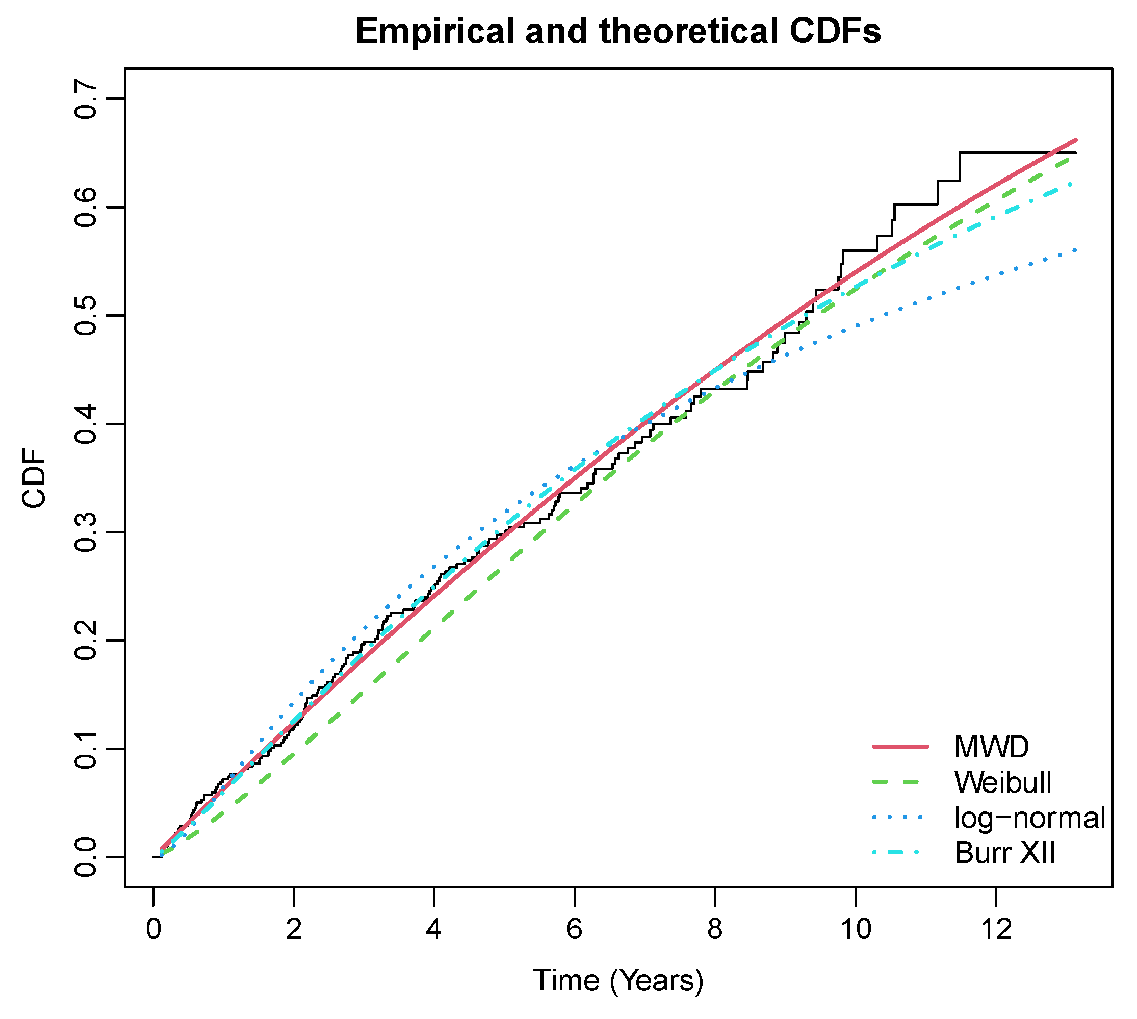
Model	MLE	Log-Likelihood	AIC	BIC
MWD	$a=0.0639$, $\alpha =0.9986$, $\lambda =0.0197$	−580.870	1167.74	1179.85
Weibull	Shape = 1.24, Scale = 12.67,	−584.0561	1172.11	1180.18
Log-normal	Meanlog = 2.341, Sdlog = 1.546	−585.9771	1175.95	1184.03
Burr XII	a = 28.53 $\alpha =1.135$, $\lambda =2.814$	−581.64	1169.28	1181.39

Figure 1. Fitted and empirical CDF plots of death for PBC data.

To transform survival time in terms of years, we divided it by 365, which yielded a median survival time 4.74 years. We also assumed that 106 patients who did not participate in the trial received the D-penicillamine treatment. Furthermore, we applied the proposed estimation methods to obtain the estimates of the unknown parameters and cumulative CSH functions. To choose unknown parameters for priors, we first tried several parameters and then chose the best one in terms of the convergence performance and computing time. Based on the results of this preliminary analysis, we decided to use the following parameters: $q_{1j}=q_{2j}=q_{3j}=1.5,r_{1j}=r_{2j}=r_{3j}=2.2$ (gamma prior); $k_{1j}=k_{2j}=k_{3j}=2,{\theta }_{1j}={\theta }_{2j}={\theta }_{3j}=0.71$ (Weibull prior); ${\mu }_{1j}={\mu }_{2j}={\mu }_{3j}=0.1,{\sigma }_{1j}={\sigma }_{2j}={\sigma }_{3j}=1$ (log-normal prior); and $c_{1j}=0,d_{1j}=1$ (uniform prior). The results of the estimates of the unknown parameters are presented in Table 4. We estimated the cumulative CSH functions using (5) based on the proposed estimators which are presented in Figure 2 and Figure 3.

Table 4. ML and Bayes parameter estimates of the modified Weibull CSAH model for transplant and death for the PBC data.

	Transplant				Death
Method	${\mathit{a}}_1$	${\mathit{\alpha }}_1$	${\mathit{\lambda }}_1$	${\mathit{\beta }}_{11}$	${\mathit{a}}_2$	${\mathit{\alpha }}_2$	${\mathit{\lambda }}_2$	${\mathit{\beta }}_{21}$
MLE	0.0117	0.3038	0.1394	0.0026	0.0407	0.2946	0.2174	0.0286
MLE.SE	0.0054	0.9331	0.1965	0.0077	0.0101	0.0947	0.0353	0.0096
G-self	0.0062	0.9640	0.0852	0.0042	0.0600	0.8965	0.0443	0.0118
G-llf1	0.0062	0.8806	0.0827	0.0042	0.0599	0.8867	0.0439	0.0117
G-llf2	0.0062	1.0445	0.0878	0.0042	0.0601	0.9061	0.0447	0.0118
G.SE	0.0031	0.3312	0.0581	0.0030	0.0109	0.1136	0.0234	0.0079
W-self	0.0062	0.9681	0.0878	0.0040	0.0597	0.8828	0.0485	0.0118
W-llf1	0.0062	0.9057	0.0859	0.0040	0.0597	0.8737	0.0481	0.0117
W-llf2	0.0062	1.0295	0.0898	0.0040	0.0598	0.8919	0.0488	0.0118
W.SE	0.0030	0.2876	0.0510	0.0029	0.0109	0.1100	0.0219	0.0080
LN-self	0.0110	0.6324	0.1081	0.0036	0.0617	0.8262	0.0597	0.0118
LN-llf1	0.0110	0.5906	0.1066	0.0036	0.0616	0.8184	0.0594	0.0117
LN-llf2	0.0110	0.6756	0.1096	0.0036	0.0618	0.8339	0.0600	0.0118
LN.SE	0.0041	0.2384	0.0449	0.0027	0.0108	0.1018	0.0205	0.0080

SE: Standard error.

Figure 2. Estimated cumulative CSH for transplant based on the Bayes estimates for informative priors and MLE based on the PBC data.

Figure 3. Estimated cumulative CSH for death based on the Bayes estimates for informative priors and MLE based on the PBC data.

These plots indicate that the cumulative CSH rate for transplant patients is small compared to the same for the patients who experienced death. Figure 2 shows that the value of the cumulative CSH function due to transplant is small for the patients who received the placebo treatment. Similarly, the same is observed for the cumulative CSH rate due to death, see Figure 3. Moreover, the likelihood ratio test procedure was also used to test the significance of the treatment effect on transplant and death separately. The hypotheses of interest are $H_0:{\beta }_{11}=0$ against $H_1:{\beta }_{11}\ne 0$ and $H_0:{\beta }_{21}=0$ against $H_1:{\beta }_{21}\ne 0$. We calculated the likelihood ratio test statistics and corresponding p-values to be $5.44\times {10}^{-06}$ and $1.02\times {10}^{-03}$. Hence, both the null hypothesis are rejected. This indicates that treatment had a significant effect on transplant and death.

To test the overall goodness of fit of the model (1) to the PBC data in competing risks framework, we used the Cox–Snell residual plot [42]. The Cox–Snell residual is defined as:

$$r_i=\widehat{H}\left(t_i\right|x_i),i=1,2,\dots ,n,$$

(24)

where $\widehat{H}\left(t\right|x)$ is the estimator of cumulative CSH rate $H\left(t\right|x)={\sum }_{j=1}^2{H}_j\left(t\right|x)$ and $j=1,2$ based on MLE for transplant and death, respectively. If the model holds, then these residuals should be a sample from a unit exponential distribution. Therefore, the hazard plot of residuals versus the Nelson–Aalen estimator of the cumulative hazard of the residuals will be a straight line with a slope equal to one. The residual plot of Figure 4 demonstrates a reasonable fit of the model (1). Readers are referred to Figures 12.6–12.9 of the book [42] for a reasonable fit.

Figure 4. Plot of the Cox–Snell residual versus its estimates of cumulative hazard rate.

8. Conclusions

In this article, we propose a parametric cause-specific AH regression analysis, where the baseline CSH functions follow the MWD. The proposed AH model is a good alternative to the Cox PH model, and it is useful when excess risk is of concern. The estimation of the unknown parameters and cumulative CSH function is dealt with by ML and Bayes estimates. In addition to Bayes estimation, we propose three types of informative priors for baseline parameters, and uniform priors are considered for regression parameters. The simulation results show that the Bayes estimates based on each considered priors under the SELF and LLF dominate over MLE for a small sample size. Furthermore, across the priors, the choice of baseline log-normal priors gives better results with a smaller MSE and AVL. Moreover, selecting different priors and loss functions shows their applicability in the simulation study. We demonstrate the model utility with the PBC data. These data fit well with the model, and the covariate significantly affects transplant and death.

The proposed work can be extended for different censoring schemes such as interval, current status, and middle censoring schemes [7,9,18,42]. Furthermore, the situation of masking in competing risks analysis is widespread [43,44]. Therefore, the analysis of masked competing risks data using the proposed model seems to be an interesting attempt.

Determining the appropriate form of the prior is often difficult, historically affecting the widespread use of the Bayesian paradigm. According to [45], there is no hard and fast rule for selecting the best possible prior distribution to formulate the Bayes estimator. In this study, we considered an informative prior for the unknown parameters. However, a noninformative prior can be used when only limited or vague knowledge (a priori) about the parameters is available. The rationale for using noninformative prior distributions is often said to be to let the data speak for themselves so that inferences are unaffected by external information to the current data. Hence, all resulting inferences were completely objective rather than subjective. A commonly used noninformative prior in Bayesian analysis is Jeffrey’s prior [46]. However, the half-t [47] distribution as a noninformative prior is also gaining attention of researchers. The proposed study can be extended for the noninformative priors which would be reported elsewhere.

References

- Cox, D.R. Regression models and life-tables. J. R. Stat. Soc. Ser. Methodol. 1972, 34, 187–220. [Google Scholar] [CrossRef]
- Cox, D.R.; Oakes, D. Analysis of Survival Data; Chapman and Hall/CRC: London, UK, 1984. [Google Scholar]
- Breslow, N.E.; Day, N.E. Statistical Methods in Cancer Research; International Agency for Research on Cancer: Lyon, France, 1987; Volume 2. [Google Scholar]
- Aalen, O.O. A linear regression model for the analysis of life times. Stat. Med. 1989, 8, 907–925. [Google Scholar] [CrossRef]
- Lin, D.; Ying, Z. Semiparametric analysis of the additive risk model. Biometrika 1994, 81, 61–71. [Google Scholar] [CrossRef]
- Lin, D.; Ying, Z. Semiparametric analysis of general additive-multiplicative hazard models for counting processes. Ann. Stat. 1995, 23, 1712–1734. [Google Scholar] [CrossRef]
- Kalbfleisch, J.D.; Prentice, R.L. The Statistical Analysis of Failure Time Data; John Wiley & Sons: Hoboken, NJ, USA, 2002; Volume 360. [Google Scholar]
- Haller, B.; Schmidt, G.; Ulm, K. Applying competing risks regression models: An overview. Lifetime Data Anal. 2013, 19, 33–58. [Google Scholar] [CrossRef]
- Lawless, J.F. Statistical Models and Methods for Lifetime Data; John Wiley & Sons: Hoboken, NJ, USA, 2003; Volume 362. [Google Scholar]
- Pintilie, M. Competing Risks: A Practical Perspective; John Wiley & Sons: Chichester, UK, 2006; Volume 58. [Google Scholar]
- Emura, T.; Shih, J.H.; Ha, I.D.; Wilke, R.A. Comparison of the marginal hazard model and the sub-distribution hazard model for competing risks under an assumed copula. Stat. Methods Med. Res. 2020, 29, 2307–2327. [Google Scholar] [CrossRef]
- Meng, C.; Esserman, D.; Li, F.; Zhao, Y.; Blaha, O.; Lu, W.; Wang, Y.; Peduzzi, P.; Greene, E.J. Simulating time-to-event data subject to competing risks and clustering: A review and synthesis. Stat. Methods Med. Res. 2023, 32, 305–333. [Google Scholar] [CrossRef] [PubMed]
- Zuo, Z.; Wang, L.; Lio, Y. Reliability estimation for dependent left-truncated and right-censored competing risks data with illustrations. Energies 2023, 16, 62. [Google Scholar] [CrossRef]
- Jeong, J.H.; Fine, J.P. Parametric regression on cumulative incidence function. Biostatistics 2007, 8, 184–196. [Google Scholar] [CrossRef]
- Anjana, S.; Sankaran, P. Parametric analysis of lifetime data with multiple causes of failure using cause specific reversed hazard rates. Calcutta Stat. Assoc. Bull. 2015, 67, 129–142. [Google Scholar] [CrossRef]
- Lee, M. Parametric inference for quantile event times with adjustment for covariates on competing risks data. J. Appl. Stat. 2019, 46, 2128–2144. [Google Scholar] [CrossRef]
- Lipowski, C.; Lo, S.; Shi, S.; Wilke, R.A. Competing risks regression with dependent multiple spells: Monte Carlo evidence and an application to maternity leave. Jpn. J. Stat. Data Sci. 2021, 4, 953–981. [Google Scholar] [CrossRef]
- Rehman, H.; Chandra, N. Inferences on cumulative incidence function for middle censored survival data with Weibull regression. Jpn. J. Stat. Data Sci. 2022, 5, 65–86. [Google Scholar] [CrossRef]
- Shen, Y.; Cheng, S. Confidence bands for cumulative incidence curves under the additive risk model. Biometrics 1999, 55, 1093–1100. [Google Scholar] [CrossRef] [PubMed]
- Sun, J.; Sun, L.; Flournoy, N. Additive hazards model for competing risks analysis of the case-cohort design. Commun. Stat. Theory Methods 2004, 33, 351–366. [Google Scholar] [CrossRef]
- Zhang, X.; Akcin, H.; Lim, H.J. Regression analysis of competing risks data via semi-parametric additive hazard model. Stat. Methods Appl. 2011, 20, 357–381. [Google Scholar] [CrossRef]
- Li, W.; Xue, X.; Long, Y. An additive subdistribution hazard model for competing risks data. Commun. Stat. Theory Methods 2017, 46, 11667–11687. [Google Scholar] [CrossRef]
- Sankaran, P.; Prasad, S. Additive risks regression model for middle censored exponentiated-exponential lifetime data. Commun. Stat. Simul. Comput. 2018, 47, 1963–1974. [Google Scholar] [CrossRef]
- Lai, C.; Xie, M.; Murthy, D. A modified Weibull distribution. IEEE Trans. Reliab. 2003, 52, 33–37. [Google Scholar] [CrossRef]
- Byrnes, J.M.; Lin, Y.J.; Tsai, T.R.; Lio, Y. Bayesian inference of δ= P (X< Y) for Burr type XII distribution based on progressively first failure-censored samples. Mathematics 2019, 7, 794. [Google Scholar]
- Martz, H.F.; Waller, R. Bayesian Reliability Analysis; John Wiley & Sons: New York, NY, USA, 1982. [Google Scholar]
- Ranjan, R.; Sen, R.; Upadhyay, S.K. Bayes analysis of some important lifetime models using MCMC based approaches when the observations are left truncated and right censored. Reliab. Eng. Syst. Saf. 2021, 214, 107747. [Google Scholar] [CrossRef]
- Ng, H.K.T. Parameter estimation for a modified Weibull distribution, for progressively type-II censored samples. IEEE Trans. Reliab. 2005, 54, 374–380. [Google Scholar] [CrossRef]
- Jiang, H.; Xie, M.; Tang, L. Markov chain Monte Carlo methods for parameter estimation of the modified Weibull distribution. J. Appl. Stat. 2008, 35, 647–658. [Google Scholar] [CrossRef]
- Upadhyay, S.; Gupta, A. A Bayes analysis of modified Weibull distribution via Markov chain Monte Carlo simulation. J. Stat. Comput. Simul. 2010, 80, 241–254. [Google Scholar] [CrossRef]
- Nelder, J.A.; Mead, R. A simplex method for function minimization. Comput. J. 1965, 7, 308–313. [Google Scholar] [CrossRef]
- Robert, C.P.; Casella, G.; Casella, G. Introducing Monte Carlo Methods with R; Springer Science & Business Media: New York, NY, USA, 2010; Volume 18. [Google Scholar]
- Geman, S.; Geman, D. Stochastic relaxation, Gibbs distributions, and the Bayesian restoration of images. IEEE Trans. Pattern Anal. Mach. Intell. 1984, PAMI-6, 721–741. [Google Scholar] [CrossRef] [PubMed]
- Hastings, W.K. Monte Carlo sampling methods using Markov chains and their applications. Biometrika 1970, 57, 97–109. [Google Scholar] [CrossRef]
- Guure, C.B.; Ibrahim, N.A. Bayesian analysis of the survival function and failure rate of Weibull distribution with censored data. Math. Probl. Eng. 2012, 2012. [Google Scholar] [CrossRef]
- Beyersmann, J.; Allignol, A.; Schumacher, M. Competing Risks and Multistate Models with R; Springer Science & Business Media: New York, NY, USA, 2012. [Google Scholar]
- Knight, K. Mathematical Statistics; CRC Press: Boca Raton, FL, USA, 1999. [Google Scholar]
- Dörre, A.; Huang, C.Y.; Tseng, Y.K.; Emura, T. Likelihood-based analysis of doubly-truncated data under the location-scale and AFT model. Comput. Stat. 2021, 36, 375–408. [Google Scholar] [CrossRef]
- Lunn, D.; Jackson, C.; Best, N.; Spiegelhalter, D.; Thomas, A. The BUGS Book: A Practical Introduction to Bayesian Analysis; Chapman and Hall/CRC: Boca Raton, FL, USA, 2012. [Google Scholar]
- Therneau, T.M.; Grambsch, P.M. Modeling Survival Data: Extending the Cox Model; Springer Science & Business Media: New York, NY, USA, 2000. [Google Scholar]
- Lai, X.; Yau, K.K.; Liu, L. Competing risk model with bivariate random effects for clustered survival data. Comput. Stat. Data Anal. 2017, 112, 215–223. [Google Scholar] [CrossRef]
- Klein, J.P.; Moeschberger, M.L. Survival Analysis: Techniques for Censored and Truncated Data; Springer: New York, NY, USA, 2003. [Google Scholar]
- Fan, T.H.; Wang, Y.F.; Ju, S.K. A competing risks model with multiply censored reliability data under multivariate Weibull distributions. IEEE Trans. Reliab. 2019, 68, 462–475. [Google Scholar] [CrossRef]
- Li, Y.; Ye, J. Analysis for partially accelerated dependent competing risks model with masked data based on copula function. Commun. Stat. Simul. Comput. 2022, 1–17. [Google Scholar] [CrossRef]
- Sinha, S. Bayesian Estimation; New Age International (P) Limited Publisher: New Delhi, India, 1998. [Google Scholar]
- Jeffreys, H. Theory of Probability; Oxford University Press: London, UK, 1961. [Google Scholar]
- Gelman, A. Prior distributions for variance parameters in hierarchical models (comment on article by Browne and Draper). Bayesian Anal. 2006, 1, 515–534. [Google Scholar] [CrossRef]