Inverse Problem Numerical Analysis of Forager Bee Losses in Spatial Environment without Contamination

Abstract

We consider an inverse problem of recovering the mortality rate in the honey bee difference equation model, that tracks a forage honeybee leaving and entering the hive each day. We concentrate our analysis to the model without pesticide contamination in the symmetric spatial environment. Thus, the mathematical problem is formulated as a symmetric inverse problem for reaction coefficient at final time constraint. We use the overspecified information to transform the inverse coefficient problem to the forward problem with non-local terms in the differential operator and the initial condition. First, we apply semidiscretization in space to the new nonsymmetric differential operator. Then, the resulting non-local nonsymmetric system of ordinary differential equations (ODEs) is discretized by three iterative numerical schemes using different time stepping. Results of numerical experiments which compare the efficiency of the numerical schemes are discussed. Results from numerical tests with synthetic and real data are presented and discussed, as well.

1. Introduction

Bees play a crucial role, not only for human beings but also for all plant species they assist in pollinating. Some of the most globally significant crops rely on bees for their reproduction, as these industrious pollinators visit and fertilize such plants. Furthermore, bees actively contribute to the preservation of natural ecosystems, as their pollination activities aid in the rejuvenation of trees. This, in turn, has a positive impact on the conservation of forest biodiversity and the maintenance of various other ecosystem services. In essence, bees serve as vital regulators of food production, forest equilibrium, and micro-climate dynamics

The loss of honey bee colonies is a prevalent occurrence that has significant economic and ecological consequences. The factors responsible for this phenomenon are currently under active investigation by many researches. Many studies have identified potential contributing factors to this problem, such as pesticides, parasites, climate change, nutritional challenges, etc. [1,2,3,4,5,6,7,8,9,10].

Remarkably, it is recognized that the development of mathematically tractable models is crucial for obtaining valuable insights into the ecological processes and factors that result in colony losses.

The pioneering mathematical model that integrated colony population dynamics influenced by biological and environmental factors was formulated in [11]. Subsequent honeybee mathematical models have been introduced, concerning the activities inside beehives, models investigating the influence of Varroa mites, models that simulate the dynamics of honeybees gathering nectar and pollen to support colony growth, models that gain valuable insights into ecological processes and factors contributing to colony losses, etc., see, e.g., review papers [2,12]. In all these models, the honeybee population dynamics are governed by ordinary differential equations (ODE).

Models involving partial differential equations to study honeybee colony dynamics are proposed in [13,14,15]. In [14,15], the authors model the thermoregulation process in honey bee colonies in winter using the Keller–Segel problem with a sign-changing chemotactic coefficient. The focus of the investigation in [13] is the exposure of forager bees to pesticides within contaminated spatial settings. The model comprises both differential and difference equations governing the spatial patterns of forager bees, distinguishing between those unaffected by contamination and those affected by it. An essential aspect of this model involves the daily return of forager bees to their hive.

Numerical simulations to study honeybee ODE problems are used in many papers. For example, in [16], critical hive sizes were determined numerically across various scenarios, emphasizing the significance of expedited forager recruitment in the depletion of hives during colony collapse. Both adult and immature honeybee populations along with their honey production are examined in [17]. For more details about the existing investigations, see also [2,12].

A second order in space, positivity-preserving numerical method for solving the Keller–Segel problem modeling the thermoregulation in honeybee colonies during the winter is developed in [18].

Over the past few decades, inverse problems have been employed to investigate numerous real-world phenomena and processes. This is primarily due to their robust mathematical formulation, comprehensive theoretical analysis, and effective numerical solutions [19,20,21,22,23,24,25,26,27].

The numerical method for solving the inverse bio-heat transfer problem for identifying space- and time-dependent perfusion coefficient from temperature measurements is constructed in [28]. The parameter identification inverse problem for a system of non-linear ODE modeling honeybee population dynamics taking into account different factors is studied in the literature; see [29,30] and reference therein. In [29], the authors consider a model describing the time evolution of the population count of hive bees, foraging workers, and contaminated foragers. A new problem for interaction of the food stock with the brood, adult bees and produced honey is suggested and analyzed numerically in [30].

Numerical identification approaches for predicting the optimal parameters governing the population dynamics in the beehive in the Keller–Segel problem under temperature measurements are developed in [31,32].

Inverse problems for recovering space-dependent mortality rate of the bees and the rate of contamination of the forager bees by pesticides under final time measurements are posed in [33].

In this work, we consider the inverse problem for recovering space-dependent reaction coefficient and solution, under final time measurements, in the Dirichlet parabolic problem. Such mathematical model is constructed in [13] to describe the spatial distribution of uncontaminated foraging bees, where the unknown solution is the bee density and the reaction coefficient represents the mortality rate of the bees. Determination of the honeybee mortality rate is of great importance for monitoring, studying the dynamics of the bee populations and developing good beekeeping practices.

We transform the inverse problem to a Dirichlet forward problem for non-local parabolic equation and non-local initial condition. Then, we further develop the iteration approach proposed in [34,35,36,37,38,39], where, in contrast to our problem, only initial conditions are non-local.

The remaining part of the paper is organized as follows. In the next section, we present the model problem. The inverse problem is formulated and discussed in Section 3. In Section 4, we construct three discrete schemes—implicit, Crank–Nicolson and averaging Saulyev’s scheme—for solving the 1D inverse problem, and on this base, we develop an iterative algorithm. In Section 5, we extend this iteration method for a 2D inverse problem. Computational results with synthetic and real data are presented in Section 6. Finally, in Section 7, we offer a summary and concluding remarks.

2. Model Problem

In this section, motivated by the results in [13], we formulate the model problem. This is a parabolic equation with Dirichlet boundary conditions that can be used to describe the spatial bee density of forage bees. We briefly discuss the model suggested in [13].

The basic assumption is that the environment is free from pesticide contamination. Forage bees depart from the hive at sunrise and come back to the hive after sunset on a daily basis.

We consider the spatial probability density function of forager bees in the hive $G(t^{*},x,y)$ for a given $t^{*}$:

$$\underset{R^2}{\int }\int G(t^{*},x,y)dxdy=1,\mathrm{for}{t}^{*}>0,$$

where G is Gaussian function

$$G(t^{*},x,y)=\frac{1}{4\pi \epsilon t^{*}}exp\left(-\frac{{(x-x_0)}^2+{(y-y_0)}^2}{4\epsilon t^{*}}\right)$$

(1)

with the standard derivation of G for a given value of $\epsilon$ and $t^{*}$ defined by $\sigma =\sqrt{2\epsilon t^{*}},$ and $(x_0,y_0)$ is the center of the hive.

Let us denote by $u(t,x,y)$ the forager bee density at time t and location $(x,y)\in R^2$.

At the beginning of the first day, the initial distribution of forager bees is

$$u(0,x,y)=u_0(x,y)\ge 0,u_0\in L_{+}^1\left(R^2\right),$$

(2)

and the total number of forager bees (TNFB) at time $t=0$ is given by

$$U_0=\underset{R^2}{\int }\int u_0(x,y)dxdy.$$

Then, the forage bee density u satisfies equation

$$\begin{array}{c}\hfill \frac{\partial u}{\partial t}=d▵u-\mu u,▵u=\frac{{\partial }^{2}u}{\partial x^2}+\frac{{\partial }^{2}u}{\partial y^2},t\in [0,t),(x,y)\in R^2,\end{array}$$

(3)

where

$$U\left(t\right)=\underset{R^2}{\int }\int u(t,x,y)dxdy$$

(4)

is the the total number of forager bees at time $t\in [0,1)$. Here, d denotes diffusion rate and $\mu (x,y)\ge 0$ is bee mortality rate. It encompasses homing failure and all other factors contributing to mortality in forager bees, and it is assumed in [13] that $\mu (x,y)$ is a bounded continuous nonnegative function on $R^2$.

At the conclusion of the initial day, we presume that all forager bees not affected by mortality make their way back to the hive, resulting in the total population at the end of the first day

$$U\left(1^{-}\right)=\underset{R^2}{\int }\int u(1^{-},x,y)dxdy.$$

The forager bees that come back to the hive during the first day actively assist in caring for the hive’s young bees. The Allee function is used to characterize how they contribute to the emergence of forager bees that subsequently depart the hive for foraging:

$$\frac{\beta U{\left(1^{-}\right)}^2}{{\mathcal{X}}^2+U{\left(1^{-}\right)}^2},$$

(5)

where $\beta$ is the maximal production parameter and $\mathcal{X}$ is the sigmoidal Hill function production [40,41].

Among forager bees, two types of behaviors emerge as they return home at the end of the day and prepare for another day of foraging. A portion of foragers return to the hive, essentially starting anew the next day without any memory of their prior day’s whereabouts. We describe their foraging pattern on the subsequent day using a diffusion model. The second behavior involves foragers that remember productive foraging sites from the prior day. The next morning, these bees head directly to these remembered locations.

Integrating these two behavioral modes and under the assumption that forager bees spread within the hive according to the Gaussian probability density $G(t^{*},x,y)$, we calculate $u_1(x,y)$. This function illustrates the spatial distribution of forager bees within the hive during the morning of the second day.

$$u_1(x,y)=G(t^{*},x,y)\left(\frac{\beta U{\left(1^{-}\right)}^2}{{\mathcal{X}}^2+U{\left(1^{-}\right)}^2}+(1-q)U\left(1^{-}\right)\right)+qu(1^{-},x,y),q\in [0,1],$$

where q is the fraction of forager bees that follow the second type of behavior. The portion of forager bees exhibiting this second behavior type consists of individuals with the ability to recall advantageous foraging sites from the prior day. When the next day begins, these bees immediately head towards these locations.

In this work, we consider Problems (2) and (3) defined in domain ${\overline{Q}}_T=\overline{\mathsf{\Omega }}\times [0,T]$, $\overline{\mathsf{\Omega }}=[0,X]\times [0,Y]$ with Dirichlet boundary conditions

$$\begin{array}{c}\hfill \begin{array}{cc}& u(t,0,y)=u_l(t,y),u(t,X,y)=u_r(t,y),y\in [0,Y],t\in (0,T],\hfill \\ & u(t,x,0)=v_d(t,x),u(t,x,Y)=v_u(t,x),x\in [0,X],t\in (0,T].\hfill \end{array}\end{array}$$

(6)

3. The Inverse Problem

In this section, we discuss the posing of the inverse problem for recovering reaction space-dependent unknown coefficients $\mu (x,y)$ in parabolic Equation (3) with measurements at the final time $t=T$ as it is performed in [33].

We consider Equation (3) at final time constraint

$$u(T,x,y)=\phi (x,y),\phi (x,y)>0,(x,y)\in \mathsf{\Omega },$$

(7)

where at first day $T=1$, and at second day $T=2$.

Frequently, despite the rapid advancements in electronic technology, beekeepers encounter challenges in obtaining adequate observational data to model forager bee behavior in food fields. We now utilize the observations stated in Equation (7) to approximately determine $u(t,x,y)$ by solving the inverse problem.

Equation (3), equipped with known coefficient d and $\mu$ and provided with suitable initial and boundary conditions, is referred to as the direct problem.

The focus of the present work is to find $\mu (x,y)$ that satisfy Equation (3) and Observation (7). We consider the case of

$$v(t,x,y)=\frac{\partial u}{\partial t}(t,x,y),(t,x,y)\in {\overline{Q}}_T.$$

(8)

Differentiating Equation (3) with respect to t, we derive

$$\frac{\partial v}{\partial t}=d▵v-\mu (x,y)v=0.$$

(9)

From Equation (3) and Observations (7), we find

$$\mu (x,y)=\frac{-\frac{\partial u}{\partial t}(T,x,y)+d▵\phi (x,y)}{\phi (x,y)}=\frac{-v(T,x,y)+d▵\phi (x,y)}{\phi (x,y)}.$$

(10)

Thus, Problems (2), (3), (6) and (7) are equivalent to the following inverse problem, formulated as a direct problem for unknown solution $v(t,x,y)$, $(x,y)\in \mathsf{\Omega }=(0,X)\times (0,Y)$, $0<t\le T$:

$$\begin{array}{c}\hfill \begin{array}{cc}\hfill & \frac{\partial v}{\partial t}=d▵v+\frac{v(T,x,y)-d▵\phi (x,y)}{\phi (x,y)}v,\hfill \\ & v(0,x,y)=d▵u_0(x,y)+\frac{v(T,x,y)-d▵\phi (x,y)}{\phi (x,y)}{u}_0(x,y),\hfill \end{array}\end{array}$$

(11)

with Dirichlet boundary conditions, derived from (6), applying (8),

$$\begin{array}{c}\hfill \begin{array}{cc}\hfill & v(t,0,y)=v_l(t,y),v(t,X,y)=v_r(t,y),y\in [0,Y],t\in (0,T],\hfill \\ & v(t,x,0)=v_d(t,x),v(t,x,Y)=v_u(t,x),x\in [0,X],t\in (0,T].\hfill \end{array}\end{array}$$

(12)

Using the results of [33] (Section 3), the following assertion can easily be proven.

Theorem 1.

Let us assume that $\phi (x,y)\in C^{4+\gamma }\left(\mathsf{\Omega }\right)$, $0<\gamma <1$ and $\phi (x,y)>0$ in $\overline{\mathsf{\Omega }}$. Then, there exists at least one solution of Problems (9)–(12).

Corollary 1.

Under the assumptions of Theorem 1, inverse Problems (3) and (7) have at least one solution.

Proof. 

Indeed, we saw that if $u(t,x,y)$ is a solution of Problems (3) and (7) with zero Dirichlet boundary conditions, then $v(t,x,y)$ is a solution to Problems (11) and (12). Conversely, assuming that $u(t,x,y)$ is a solution of Problems (3) and (7), it follows that

$$u(t,x,y)=u_0(x,y)+\underset{0}{\overset{t}{\int }}v(\lambda ,x,y)d\lambda ,\mu (x,y)=\frac{-v(T,x,y)+d▵\phi (x,y)}{\phi (x,y)}$$

is a solution of inverse Problems (3) and (7) with zero Dirichlet boundary conditions. □

4. Iterative Method for Solving a 1D Inverse Problem

In this section, we propose three numerical iterative schemes for solving Problems (11) and (12). For clarity, first, we explain the method for the following one-dimensional prototype problem of (11) and (12):

$$\begin{array}{ccc}& & \frac{\partial v}{\partial t}=d\frac{{\partial }^{2}v}{\partial x^2}+\frac{v(T,x)-d\frac{d^2\phi }{d{x}^2}}{\phi \left(x\right)}v,(x,t)\in Q_T=\mathsf{\Omega }\times (0,T],\hfill \\ \hfill & & v(t,0)=v_l\left(t\right),v(t,x)=v_r\left(t\right),0<t\le T,\hfill \\ & & v(0,x)=d\frac{d^2{u}_0\left(x\right)}{d{x}^2}+\frac{v(T,x)-d\frac{d^2\phi }{d{x}^2}}{\phi \left(x\right)}{u}_0\left(x\right),x\in \mathsf{\Omega }=(0,X).\hfill \end{array}$$

(13)

For the solution of (13), we construct iterative finite difference methods using ideas from papers [34,36,37,38,39], where linear parabolic problems with non-local terms only in the initial condition are solved.

4.1. Discrete Schemes

We introduce uniform partition of the interval $[0,X]$. We let $h>0$ be small and $x_i=ih,i=0,1,\dots ,I$, where $I=X/h$ is a positive integer.

The semi-discrete solution $v_i\left(t\right)=v(x_i,t)$ of (13) satisfies the following ODE system:

$$\begin{array}{c}\hfill \begin{array}{cc}\hfill & \frac{\partial v_i}{\partial t}=d{▵}_h{v}_i+\frac{v_i\left(T\right)-d{▵}_h{\phi }_i}{{\phi }_i}{v}_i,i=1,2,\dots ,I-1,\hfill \\ & v_0=v_l\left(t\right),v_I=v_r\left(t\right),\hfill \\ & v_i\left(0\right)=d{▵}_h{\left(u_0\right)}_i+\frac{v_i\left(T\right)-d{▵}_h{\phi }_i}{\phi \left(x_i\right)}{\left(u_0\right)}_i,i=1,2,\dots ,I-1.\hfill \end{array}\end{array}$$

(14)

In the time interval $[0,T]$, we define the uniform grid with nodes $t_k=k\tau$, $k=0,1,\dots ,K$, $\tau =T/K$. The values of the solution and mesh functions at grid nodes are denoted by $w_i^k=w(x_i,t_k)$.

Further, we apply three different temporal discretizations for the ODE system (14).

• The implicit backward Euler scheme: we find $\left\{v_i^k\right\}$, $k=1,2,\dots ,K$ such that

  $$\begin{array}{c}\hfill \begin{array}{cc}\hfill & \frac{v_i^k-v_i^{k-1}}{\tau }=d{▵}_h{v}_i^k+\frac{v_i^K-d{▵}_h{\phi }_i}{{\phi }_i}{v}_i^k,i=1,2,\dots ,I-1,\hfill \\ & v_0^k=v_l\left(t_k\right),v_I^k=v_r\left(t_k\right),\hfill \\ & v_i^0=d{▵}_h{\left(u_0\right)}_i+\frac{v_i^K-d{▵}_h{\phi }_i}{\phi \left(x_i\right)}{\left(u_0\right)}_i,i=1,2,\dots ,I-1,\hfill \end{array}\end{array}$$

  (15)

  where ${▵}_h{w}_i^k=(w_{i+1}^k-2w_i^k+w_{i-1}^k)/h^2$.
• The Crank–Nicolson scheme. Now, $\left\{v_i^k\right\}$, $k=1,2,\dots ,K$ is defined by

  $${\displaystyle \frac{v_i^k-v_i^{k-1}}{\tau }=d{▵}_h\frac{v_i^k+v_i^{k-1}}{2}+\frac{v_i^K-d{▵}_h{\phi }_i}{{\phi }_i}\frac{v_i^k+v_i^{k-1}}{2},i=1,2,\dots ,I-1,}$$

  (16)

  with the same initial and boundary approximate conditions as above.
• The Saulyev-type alternating direction explicit (ADE) scheme. For the approximation, we use Saulyev’s first- and second-kind formula in order to obtain an unconditional stable numerical scheme, which can be realized in an explicit manner.

In discrete Scheme (15), we replace ${▵}_h{v}_i^k$ by ${▵}_h^1{v}_i^k=(v_{i-1}^k-v_i^{k-1}-v_i^k+v_{i+1}^{k-1})/h^2$ and ${▵}_h^2{v}_i^k=(v_{i+1}^{k-1}-v_i^{k-1}-v_i^k+v_{i-1}^k)/h^2$. In order to obtain better accuracy, we combine these approximations and derive the Barakat and Clark scheme.

We find $\left\{v_i^k\right\}$ at each time layer $k=1,2,\dots ,K$, as an averaging solution of numerical schemes

$$\begin{array}{c}\hfill \begin{array}{cc}\hfill & \frac{v_i^k-v_i^{k-1}}{\tau }=d{▵}_h^1{v}_i^k+\frac{v_i^K-d{▵}_h{\phi }_i}{{\phi }_i}{v}_i^k,i=I-1,I-2,\dots ,1,\hfill \\ & \frac{v_i^k-v_i^{k-1}}{\tau }=d{▵}_h^2{v}_i^k+\frac{v_i^K-d{▵}_h{\phi }_i}{{\phi }_i}{v}_i^k,i=1,2,\dots ,I-1,\hfill \\ & v_0^k=v_l\left(t_k\right),v_I^k=v_r\left(t_k\right),\hfill \\ & v_i^0=d{▵}_h{\left(u_0\right)}_i+\frac{v_i^K-d{▵}_h{\phi }_i}{{\phi }_i}{\left(u_0\right)}_i,1\le i\le I-1.\hfill \end{array}\end{array}$$

(17)

In general, implicit methods require more computational efforts, but they are unconditionally stable. Moreover, the fully implicit scheme is first-order accurate in time, while the Crank–Nicolson scheme is second-order accurate both in space and time. However, it is known that in some cases, the Crank–Nicolson method may produce oscillations in the numerical solution [42]. On the other hand, Saulyev’s first- and second-kind formulas are unconditionally stable, can be computed in an explicit manner, but they are first-order accurate. To enhance the order of convergence, we need to construct the Barakat and Clark scheme, which couples these two approximations.

There are many other methods that can be used; for example, the unconditionally stable Dufort–Frankel scheme, which is a three-level, second- or fourth-order accurate in space for appropriate choice of the mesh parameters [43]; explicit and unconditionally stable odd–even hopscotch scheme; leapfrog hopscotch scheme and hybrid schemes, combining the above methods. New results in this direction are obtained in [44,45,46,47].

Now, we state our stability and convergence results. We denote by $\parallel w\parallel =\underset{0\le i\le I}{max}\left|w_i\right|$.

Theorem 2.

We let $\left\{v_i^k\right\}$ be the solution of the backward Euler or Crank–Nicolson scheme; then, there exists a constant $C>0$, independent of τ and h and ${\tau }_0>0$, such that for all $0<\tau \le {\tau }_0$, we have

$$\begin{array}{c}\hfill \begin{array}{cc}\hfill & \underset{0\le k\le K}{max}\parallel v\left(t_k\right)-V^k\parallel \le C(\tau +h^2),\hfill \\ & \underset{0\le k\le K}{max}\parallel V^k\parallel \le C\sum _{k=0}^K\tau \left(\right|v_l\left(t_k\right)|+|v_r\left(t_k\right)\left|\right),\hfill \end{array}\end{array}$$

(18)

where $V^k={(V_1^k,V_2^k,\dots ,V_{I-1}^k)}^T$.

4.2. Iterative Procedure

To solve Problem (15) for identifying $v^k$, $k=1,2,\dots ,K$, we use Discretizations (15)–(18) and in order to avoid solving large non-linear systems of algebraic equations, we initiate an iteration procedure. As an initial guess, we set ${\left(v_i^0\right)}^{\left(0\right)}=0$, $i=0,1,\dots ,I$. Then, ${\left(v_i^0\right)}^{(l+1)}$, $l=0,1,\dots$, $i=0,1,\dots ,I$ is determined by

$${\left(v_i^0\right)}^{(l+1)}=d{▵}_h{\left(u_0\right)}_i+\frac{{\left(v_i^K\right)}^{\left(l\right)}-d{▵}_h{\phi }_i}{{\phi }_i}{\left(u_0\right)}_i,i=1,2,\dots ,I-1,$$

where ${\left(v_i^k\right)}^{\left(l\right)}$, $k=1,2,\dots ,K$ is the solution of the following problems, denoting $v_i^k={\left(v_i^k\right)}^{(l+1)}$ for simplicity, depending on the scheme used:

• (IMIS-1D) Iteration method based on the implicit backward Euler scheme (15):

  $$\begin{array}{c}\hfill \begin{array}{cc}\hfill & \frac{v_i^k-v_i^{k-1}}{\tau }=d{▵}_h{u}_i^k+\frac{{\left(v_i^K\right)}^{\left(l\right)}-d{▵}_h{\phi }_i}{{\phi }_i}{v}_i^k,i=1,2,\dots ,I-1,\hfill \\ & v_0^k=v_l\left(t_k\right),v_I^k=v_r\left(t_k\right),\hfill \\ & v_i^0={\left(v_i^0\right)}^{\left(l\right)}.\hfill \end{array}\end{array}$$

  (19)
• (IMCNS-1D) Iteration method based on the Crank–Nicolson scheme (16):

  $$\begin{array}{c}\hfill \begin{array}{cc}\hfill & \frac{v_i^k-v_i^{k-1}}{\tau }=d{▵}_h\frac{v_i^k+v_i^{k-1}}{2}+\frac{{\left(v_i^K\right)}^{\left(l\right)}-d{▵}_h{\phi }_i}{{\phi }_i}\frac{v_i^k+v_i^{k-1}}{2},i=1,2,\dots ,I-1,\hfill \\ & v_0^k=v_l\left(t_k\right),v_I^k=v_r\left(t_k\right),\hfill \\ & v_i^0={\left(v_i^0\right)}^{\left(l\right)}.\hfill \end{array}\end{array}$$

  (20)
• (IMBCS-1D) Iteration method based on the Barakat and Clark scheme obtained by averaging the solution of the first- and second-kind Saulyev’s scheme (17). We suppose that $v^K$ in (17) is known. Then, the first-kind approximation is explicit if the computations are performed from the left boundary to the right. Analogically, in a symmetric way, the same is performed for the second-kind approximation. The discretization is realized in an explicit manner if we compute the solution from the right to the left boundary. Therefore, taking $v^K$ to be known from previous iteration, we obtain the following iteration process based on the explicit schemes:

  $$\begin{array}{c}\hfill \begin{array}{cc}\hfill & {\left(v_1\right)}_i^k=Q_i^{-1}\left(\frac{v_i^{k-1}}{\tau }+d\frac{v_{i+1}^{k-1}-v_i^{k-1}+{\left(v_1\right)}_{i-1}^k}{h^2}\right),i=I-1,I-2,\dots ,1,\hfill \\ & {\left(v_2\right)}_i^k=Q_i^{-1}\left(\frac{v_i^{k-1}}{\tau }+d\frac{{\left(v_2\right)}_{i+1}^k-v_i^{k-1}+v_{i-1}^{k-1}}{h^2}\right),i=1,2,\dots ,I-1,\hfill \\ & Q_i=\frac{1}{\tau }+\frac{d}{h^2}+\frac{{\left(v_i^K\right)}^{\left(l\right)}-d{▵}_h{\phi }_i}{{\phi }_i},\hfill \\ & {\left(v_1\right)}_0^k=v_l\left(t_k\right),{\left(v_2\right)}_I^k=v_r\left(t_k\right),v_i^0={\left(v_i^0\right)}^{\left(l\right)},\hfill \\ & v_i^k=\frac{{\left(v_1\right)}_i^k+{\left(v_2\right)}_i^k}{2},1\le i\le I-1,v_0^k=v_l\left(t_k\right),v_I^k=v_r\left(t_k\right).\hfill \end{array}\end{array}$$

  (21)

The iteration process continues up to reaching the desired accuracy $ϵ$,

$$\parallel v^{(l+1)}-v^{\left(l\right)}\parallel \le ϵ,$$

or $\parallel v^{(l+1)}-v^{\left(l\right)}\parallel \ge \parallel v^{\left(l\right)}-v^{(l-1)}\parallel$.

Solution $u^{k+1}$ is obtained, integrating (8) at each time layer. Applying trapezoidal rule in the right-hand side, we obtain

$$u^{k+1}=u^k+\frac{\tau }{2}\left(v^{k+1}+v^k\right),k=1,2,\dots ,K.$$

(22)

Thus, the approximation of solution u is obtained by (22).

5. Iterative Method for Solving a 2D Inverse Problem

In this section, we construct the iteration procedure for solving Problems (11) and (12). First, we discretize domain $\overline{\mathsf{\Omega }}\times [0,T]$, $\overline{\mathsf{\Omega }}=[0,X]\times [0,Y]$. The mesh in time is the same as in Section 4. As before, symmetrically in the x- and y-directions, we consider uniform partition of the corresponding intervals $[0,X]$ and $[0,Y]$. We let $h_1>0$ and $h_2>0$ be small numbers. Then, $x_i=i{h}_1$, $i=0,1,\dots ,I$ and $y_j=j{h}_2$, $j=0,1,\dots ,J$, where $I=X/h_1$, $J=Y/h_2$. The numerical solution and the values of the mesh functions at grid nodes are denoted by $w_{i,j}^k=w(t_k,x_i,y_j)$.

We construct the same discretizations of Problems (11) and (12) as for the 1D case.

5.1. Discrete Schemes

• The implicit backward Euler scheme: we find $\left\{v_{i,j}^k\right\}$, $k=1,2,\dots ,K$, such that

  $$\begin{array}{c}\hfill \begin{array}{cc}\hfill & \frac{v_{i,j}^k-v_{i,j}^{k-1}}{\tau }=d{▵}_h{v}_{i,j}^k+\frac{v_{i,j}^K-d{▵}_h{\phi }_i}{{\phi }_{i,j}}{v}_{i,j}^k,i=1,2,\dots ,I-1,j=1,2,\dots ,J-1,\hfill \\ & v_{0,j}^k=v_l(t_k,y_j),v_{I,j}^k=v_r(t_k,y_j),j=1,2,\dots ,J,\hfill \\ & v_{i,0}^k=v_d(t_k,x_i),v_{i,J}^k=v_u(t_k,x_i),i=1,2,\dots ,I,\hfill \\ & v_{i,j}^0=d{▵}_h{\left(u_0\right)}_{i,j}+\frac{v_{i,j}^K-d{▵}_h{\phi }_{i,j}}{{\phi }_{i,j}}{\left(u_0\right)}_{i,j},i=1,2,\dots ,I-1,j=1,2,\dots ,J-1,\hfill \end{array}\end{array}$$

  (23)

  where ${▵}_h{w}_{i,j}^k=(w_{i+1,j}^k-2w_{i,j}^k+w_{i-1,j}^k)/h_1^2+(w_{i,j+1}^k-2w_{i,j}^k+w_{i,j-1}^k)/h_2^2$.
• The Crank–Nicolson scheme. We find $\left\{v_{i,j}^k\right\}$, $k=1,2,\dots ,K$, solving the system

  $${\displaystyle \frac{v_{i,j}^k-v_{i,j}^{k-1}}{\tau }=d{▵}_h\frac{v_{i,j}^k+v_{i,j}^{k-1}}{2}+\frac{v_{i,j}^K-d{▵}_h{\phi }_{i,j}}{{\phi }_{i,j}}\frac{v_{i,j}^k+v_{i,j}^{k-1}}{2},}$$

  (24)

  $i=1,2,\dots ,I-1$, $j=1,2,\dots ,J-1$, with the same initial and boundary discrete conditions as in (23).
• The ADE approximation, using the averaging of Saulyev’s first- and second-kind formulae. In discrete scheme (23), we replace ${▵}_h{v}_{i,j}^k$ by ${▵}_h^1{v}_{i,j}^k$ and ${▵}_h^2{v}_{i,j}^k$, where

  $$\begin{array}{c}\hfill {▵}_h^1{v}_{i,j}^k=\frac{v_{i+1,j}^{k-1}-v_{i,j}^{k-1}-v_{i,j}^k+v_{i-1}^k}{h_1^2}+\frac{v_{i,j+1}^{k-1}-v_{i,j}^{k-1}-v_{i,j}^k+v_{i,j-1}^k}{h_2^2},\\ \hfill {▵}_h^2{v}_{i,j}^k=\frac{v_{i+1,j}^k-v_{i,j}^{k-1}-v_{i,j}^k+v_{i-1,j}^{k-1}}{h_1^2}+\frac{v_{i,j+1}^k-v_{i,j}^{k-1}-v_{i,j}^k+v_{i,j-1}^{k-1}}{h_2^2}.\end{array}$$

We combine these approximations in order to construct the Barakat and Clark scheme. Namely, we find $\left\{v_{i,j}^k\right\}$, $k=1,2,\dots ,K$, averaging the solution of the numerical schemes at each time level

$$\begin{array}{c}\hfill \begin{array}{cc}\hfill & \frac{v_{i,j}^k-v_{i,j}^{k-1}}{\tau }=d{▵}_h^1{v}_{i,j}^k+\frac{v_{i,j}^K-d{▵}_h{\phi }_i}{{\phi }_{i,j}}{v}_{i,j}^k,i=I-1,I-2,\dots ,1,j=J-1,J-2,\dots ,1,\hfill \\ & \frac{v_{i,j}^k-v_{i,j}^{k-1}}{\tau }=d{▵}_h^2{v}_{i,j}^k+\frac{v_{i,j}^K-d{▵}_h{\phi }_{i,j}}{{\phi }_{i,j}}{v}_{i,j}^k,i=1,2,\dots ,I-1,j=1,2,\dots ,J-1,\hfill \\ & v_{0,j}^k=v_l(t_k,y_j),v_{I,j}^k=v_r(t_k,y_j),j=1,2,\dots ,J,\hfill \\ & v_{i,0}^k=v_d(t_k,x_i),v_{i,J}^k=v_u(t_k,x_i),i=1,2,\dots ,I,\hfill \\ & v_{i,j}^0=d{▵}_h{\left(u_0\right)}_{i,j}+\frac{v_{i,j}^K-d{▵}_h{\phi }_{i,j}}{{\phi }_{i,j}}{\left(u_0\right)}_{i,j},1\le i\le I-1,1\le j\le J-1.\hfill \end{array}\end{array}$$

(25)

5.2. Iterative Method

Problems (11) and (12) for finding $v^k$, $k=1,2,\dots ,K$ are solved by the iterative method, based on Discretizations (23)–(25). The initial guess is ${\left(v_{i,j}^0\right)}^{\left(0\right)}=0$, $i=0,1,\dots ,I$, $j=0,1,\dots ,J$. Then, ${\left(v_{i,j}^0\right)}^{(l+1)}$, $l=0,1,\dots$, $i=0,1,\dots ,I$, $j=0,1,\dots ,J$ is determined from

$${\left(v_{i,j}^0\right)}^{(l+1)}=d{▵}_h{\left(u_0\right)}_{i,j}+\frac{{\left(v_{i,j}^K\right)}^{\left(l\right)}-d{▵}_h{\phi }_{i,j}}{{\phi }_{i,j}}{\left(u_0\right)}_{i,j},i=1,2,\dots ,I-1,j=1,2,\dots ,J-1,$$

where ${\left(v_{i,j}^k\right)}^{\left(l\right)}$, $k=1,2,\dots ,K$ is the solution of discrete Problems (23)–(25), where, for simplicity, we denote $v_{i,j}^k={\left(v_{i,j}^k\right)}^{(l+1)}$.

• (IMIS-2D) The iteration method based on the implicit backward Euler scheme (23):

  $$\begin{array}{c}\hfill \begin{array}{cc}\hfill & \frac{v_{i,j}^k-v_{i,j}^{k-1}}{\tau }=d{▵}_h{u}_{i,j}^k+\frac{{\left(v_{i,j}^K\right)}^{\left(l\right)}-d{▵}_h{\phi }_i}{{\phi }_{i,j}}{v}_{i,j}^k,i=1,2,\dots ,I-1,j=1,2,\dots ,J,\hfill \\ & v_{0,j}^k=v_l(t_k,y_j),v_{I,j}^k=v_r(t_k,y_j),j=1,2,\dots ,J,\hfill \\ & v_{i,0}^k=v_d(t_k,x_i),v_{i,J}^k=v_u(t_k,x_i),i=1,2,\dots ,I,\hfill \\ & v_{i,j}^0={\left(v_{i,j}^0\right)}^{\left(l\right)}.\hfill \end{array}\end{array}$$

  (26)
• (IMCNS-2D) The iteration method based on the Crank–Nicolson scheme (24):

  $$\begin{array}{c}\hfill \begin{array}{cc}\hfill & \frac{v_{i,j}^k-v_{i,j}^{k-1}}{\tau }=d{▵}_h\frac{v_{i,j}^k+v_{i,j}^{k-1}}{2}\hfill \\ & +\frac{{\left(v_{i,j}^K\right)}^{\left(l\right)}-d{▵}_h{\phi }_{i,j}}{{\phi }_{i,j}}\frac{v_{i,j}^k+v_{i,j}^{k-1}}{2},i=1,2,\dots ,I-1,j=1,2,\dots ,J,\hfill \\ & v_{0,j}^k=v_l(t_k,y_j),v_{I,j}^k=v_r(t_k,y_j),j=1,2,\dots ,J,\hfill \\ & v_{i,0}^k=v_d(t_k,x_i),v_{i,J}^k=v_u(t_k,x_i),i=1,2,\dots ,I,\hfill \\ & v_{i,j}^0={\left(v_{i,j}^0\right)}^{\left(l\right)}.\hfill \end{array}\end{array}$$

  (27)
• (IMBCS-2D) The iteration method obtained by averaging the solution of the first- and the second-kind Saulyev’s scheme (25). Taking $v^K$ to be known from previous iteration, the first approximation is explicit if the computations are performed passing the nodes from the bottom boundary to the top and from the left boundary to the right. Similarly, the second-kind approximation is performed in an explicit manner if we compute the solution from the upper to the bottom boundary and from the right to the left boundary. Thus, we obtain the following iteration process based on the explicit schemes:

  $$\begin{array}{c}\hfill \begin{array}{cc}\hfill & {\left(v_1\right)}_{i,j}^k=Q_{i,j}^{-1}\left(\frac{v_{i,j}^{k-1}}{\tau }+d\frac{v_{i+1,j}^{k-1}-v_{i,j}^{k-1}+{\left(v_1\right)}_{i-1,j}^k}{h_1^2}+d\frac{v_{i,j+1}^{k-1}-v_{i,j}^{k-1}+{\left(v_1\right)}_{i,j-1}^k}{h_1^2}\right),\hfill \\ & i=I-1,I-2,\dots ,1,j=J-1,J-2,\dots ,1,\hfill \\ & {\left(v_2\right)}_{i,j}^k=Q_{i,j}^{-1}\left(\frac{v_{i,j}^{k-1}}{\tau }+d\frac{{\left(v_2\right)}_{i+1,j}^k-v_{i,j}^{k-1}+v_{i-1,j}^{k-1}}{h_1^2}+d\frac{{\left(v_2\right)}_{i,j+1}^k-v_{i,j}^{k-1}+v_{i,j-1}^{k-1}}{h_2^2}\right),\hfill \\ & i=1,2,\dots ,I-1,j=1,2,\dots ,J-1,\hfill \\ & Q_{i,j}=\frac{1}{\tau }+\frac{2d}{h^2}+\frac{{\left(v_{i,j}^K\right)}^{\left(l\right)}-d{▵}_h{\phi }_{i,j}}{{\phi }_i},\hfill \\ & {\left(v_1\right)}_{0,j}^k=v_l(t_k,y_j),{\left(v_2\right)}_{I,j}^k=v_r(t_k,y_j),j=1,2,\dots ,J,\hfill \\ & {\left(v_1\right)}_{i,0}^k=v_d(t_k,x_i),{\left(v_2\right)}_{i,J}^k=v_u(t_k,x_i),i=1,2,\dots ,I,\hfill \\ & v_{i,j}^0={\left(v_{i,j}^0\right)}^{\left(l\right)},\hfill \\ & v_{i,j}^k=\frac{{\left(v_1\right)}_{i,j}^k+{\left(v_2\right)}_{i,j}^k}{2},1\le i\le I-1,1\le j\le J-1,\hfill \\ & v_{0,j}^k=v_l(t_k,y_j),v_{I,j}^k=v_r(t_k,y_j),j=1,2,\dots ,J,\hfill \\ & v_{i,0}^k=v_d(t_k,x_i),v_{i,J}^k=v_u(t_k,x_i),i=1,2,\dots ,I.\hfill \end{array}\end{array}$$

  (28)

The iteration process continues up to reaching the desired accuracy $ϵ$:

$$\parallel v^{(l+1)}-v^{\left(l\right)}\parallel \le ϵ,\mathrm{where}\parallel w_{i,j}\parallel =\underset{0\le i\le I}{max}\underset{0\le j\le J}{max}\left|w_{i,j}\right|,$$

(29)

or $\parallel v^{(l+1)}-v^{\left(l\right)}\parallel \ge \parallel v^{\left(l\right)}-v^{(l-1)}\parallel$.

Solution u is obtained from (22).

6. Numerical Tests

In this section, we illustrate the accuracy and efficiency of the proposed iterative procedure for solving 1D and 2D inverse Problems (11)–(13).

Example 1

(1D problem: convergence test). In this test example, we verify the order of convergence of iteration methods IMIS-1D, IMCNS-1D, IMBCS-1D for solving 1D Problem (13) for given functions $u_0\left(x\right)$ and $\phi \left(x\right)$. The accuracy of these approaches is computed for modified Problem (13), $T=1$, $X=1$ with exact solution $v(t,x)=-e^{-t}sin\left(\pi x\right)$. To this aim, we add residual functions in the right-hand side of the equation in (13) and set $\phi \left(x\right)=e^{-T}sin\left(\pi x\right)$, $u_0\left(x\right)=sin\left(\pi x\right)$.

We offer the absolute errors and orders of convergence in maximal and $L_2$ norms at a final time, as well as the relative errors in the maximal discrete norm and the corresponding orders of convergence

$$\begin{array}{cc}& {\displaystyle {\mathcal{E}}_{\infty }={\mathcal{E}}_{\infty }^I=\parallel v^K-v(x,T)\parallel ,C{R}_{\infty }={log}_2\frac{{\mathcal{E}}^I}{{\mathcal{E}}^{2I}},}\\ & {\displaystyle {\mathcal{E}}_2={\mathcal{E}}_2^I=\parallel v^K{-v(x,T)\parallel }_2,C{R}_2={log}_2\frac{{\mathcal{E}}_2^I}{{\mathcal{E}}_2^{2I}},{\parallel w\parallel }_2=\sqrt{\sum _{i=0}^{I}h{w}_i^2},}\\ & {\mathcal{E}}_R={\mathcal{E}}_R^I=∥\frac{v^K-v(x,T)}{v(x,T)}∥,C{R}_R={log}_2\frac{{\mathcal{E}}_R^I}{{\mathcal{E}}_R^{2I}}.\end{array}$$

Since the expected order of convergence of IMIS-1D and IMBCS-1D is $O(\tau +h^2)$, the computations are performed for $\tau \approx h^2$. Similarly, since the expected order of convergence of IMCNS-1D is $O({\tau }^2+h^2)$, for all runs, we take $\tau \approx h$. The accuracy is $ϵ=1\times {10}^{-7}$. The results from computations are given in Table 1, Table 2 and Table 3. The number of iterations is denoted by $iter$. We observe that only a few iterations are needed to reach the desired accuracy, and because of the fixed ratio between mesh step sizes, the order of convergence is as expected.

Table 1. Errors and convergence rate of the solution of IMIS-1D, $\tau =h^2$, Example 1.

I	$\mathit{\tau }$	${\mathcal{E}}_{\mathit{\infty }}$	${\mathit{CR}}_{\mathit{\infty }}$	${\mathcal{E}}_2$	${\mathit{CR}}_2$	${\mathcal{E}}_{\mathit{R}}$	${\mathit{CR}}_{\mathit{R}}$	$\mathit{iter}$
20	2.500000 × 10−3	6.8620 × 10−4		4.8594 × 10−4		1.9222 × 10−3		4
40	6.250000 × 10−4	1.7141 × 10−4	2.0012	1.2139 × 10−4	2.0012	4.8026 × 10−4	2.0009	4
80	1.562500 × 10−4	4.2850 × 10−5	2.0001	3.0340 × 10−5	2.0002	1.2006 × 10−4	2.0002	4
160	3.906250 × 10−5	1.0713 × 10−5	1.9999	7.5846 × 10−6	2.0001	3.0010 × 10−5	2.0001	4
320	9.765625 × 10−6	2.6782 × 10−6	2.0001	1.8961 × 10−6	2.0001	7.5030 × 10−6	2.0000	4

Table 2. Errors and convergence rate of the solution of IMCNS-1D, $\tau =h$, Example 1.

I	${\mathcal{E}}_{\mathit{\infty }}$	${\mathit{CR}}_{\mathit{\infty }}$	${\mathcal{E}}_2$	${\mathit{CR}}_2$	${\mathcal{E}}_{\mathit{R}}$	${\mathit{CR}}_{\mathit{R}}$	$\mathit{iter}$
20	5.4756 × 10−4		3.8788 × 10−4		1.5432 × 10−3		6
40	1.3681 × 10−4	2.0009	9.6909 × 10−5	2.0009	3.8567 × 10−4	2.0005	5
80	3.4207 × 10−5	1.9997	2.4223 × 10−5	2.0002	9.6408 × 10−5	2.0001	5
160	8.5516 × 10−6	2.0000	6.0555 × 10−6	2.0001	2.4100 × 10−5	2.0001	4
320	2.1378 × 10−6	2.0000	1.5138 × 10−6	2.0001	6.0229 × 10−6	2.0005	4

Table 3. Errors and convergence rate of the solution of IMBCS-1D, $\tau =h^2$, Example 1.

I	${\mathcal{E}}_{\mathit{\infty }}$	${\mathit{CR}}_{\mathit{\infty }}$	${\mathcal{E}}_2$	${\mathit{CR}}_2$	${\mathcal{E}}_{\mathit{R}}$	${\mathit{CR}}_{\mathit{R}}$	$\mathit{iter}$
20	1.5768 × 10−3		1.0677 × 10−3		4.2919 × 10−3		4
40	4.3687 × 10−4	1.8517	3.0230 × 10−4	1.8204	1.1912 × 10−3	1.8493	4
80	1.1413 × 10−4	1.9366	7.98838 × 10−5	1.9200	3.1212 × 10−4	1.9322	4
160	2.9114 × 10−5	1.9708	2.0494 × 10−5	1.9627	7.9964 × 10−5	1.9647	4
320	7.3485 × 10−6	1.9862	5.1876 × 10−6	1.9821	2.0279 × 10−5	1.9794	4

Example 2

(2D problem: convergence test). Now, we verify the order of convergence of the iteration methods for solving the 2D inverse problem for identifying $u(t,x,y)$ and $\mu (x,y)$ in Equation (3) associated with zero Dirichlet boundary conditions and given observations (7). To this aim, we consider the corresponding modified problem, setting $\mu (x,y)=2x^2+y+1$ and adding residual function $f(t,x,y)$ in the right-hand side of Equation (3), such that the exact solution is $u=e^{-t}sin\left(\pi x\right)sin\left(\pi y\right)$ and $\phi (x,y)=e^{-T}sin\left(\pi x\right)sin\left(\pi y\right)$.

We solve the inverse problem by iterative methods IMIS-2D, IMCNS-2D, IMBCS-2D for $I=J$, i.e., $h_1=h_2=h$. As in Example 1, the mesh step sizes are fixed according to the expected order of convergence of the corresponding iteration method, namely $\tau \approx h^2$ for IMIS-2D and IMBCS-2D, and $\tau \approx h$ for IMCNS-2D. For the stopping criteria, we take $ϵ=1\times {10}^{-7}$.

Errors and order of convergence of the restored solution u and $\mu$, in maximal and $L_2$ norms at the final time are defined as follows:

$$\begin{array}{cc}& {\displaystyle {\mathcal{E}}_{\infty }={\mathcal{E}}_{\infty }^I=\parallel u^K-u(x,y,T)\parallel ,C{R}_{\infty }={log}_2\frac{{\mathcal{E}}^I}{{\mathcal{E}}^{2I}},}\\ & {\displaystyle {\mathcal{E}}_2={\mathcal{E}}_2^I=\parallel u^K{-u(x,y,T)\parallel }_2,C{R}_2={log}_2\frac{{\mathcal{E}}_2^I}{{\mathcal{E}}_2^{2I}},{\parallel w\parallel }_2=\sqrt{\sum _{i=0}^I\sum _{j=0}^J{h}_1{h}_2{w}_{i,j}^2},}\\ & {\displaystyle {\mathcal{E}}_{\infty }^{\mu }={\left({\mathcal{E}}^{\mu }\right)}_{\infty }^I=\parallel \mu -\mu (x,y)\parallel ,C{R}_{\infty }={log}_2\frac{{\left({\mathcal{E}}^{\mu }\right)}^I}{{\left({\mathcal{E}}^{\mu }\right)}^{2I}},}\\ & {\displaystyle {\mathcal{E}}_2^{\mu }={\left({\mathcal{E}}^{\mu }\right)}_2^I={\parallel \mu -\mu (x,y)\parallel }_2,C{R}_2={log}_2\frac{{\left({\mathcal{E}}^{\mu }\right)}_2^I}{{\left({\mathcal{E}}^{\mu }\right)}_2^{2I}}.}\end{array}$$

Since the modified problem for Equation (3) has a right-hand side $f(t,x,y)$, we also modify Equation (11) in the corresponding to (11) and (12) problems as follows:

$$\begin{array}{c}\hfill \begin{array}{cc}\hfill & \frac{\partial v}{\partial t}=d▵v+\frac{v(T,x,y)-d▵\phi (x,y)-f(t,x,y)}{\phi (x,y)}v+\frac{\partial f(t,x,y)}{\partial t},\hfill \\ & v(0,x,y)=d▵u_0(x,y)+\frac{v(T,x,y)-d▵\phi (x,y)-f(t,x,y)}{\phi (x,y)}{u}_0(x,y),\hfill \end{array}\end{array}$$

(30)

and $\mu (x,t)=[-v(T,x,y)+d▵\phi (x,y)+f(t,x,y\left)\right]/\phi (x,y)$. Similarly, iterative methods IMIS-2D, IMCNS-2D, IMBCS-2D are modified according to (30).

Computational results presented in Table 4, Table 5 and Table 6 confirm that the iteration process for recovering both reaction coefficient $\mu$ and solution u has the same order of convergence as the underlying numerical scheme.

Table 4. Errors and convergence rate of the solution of IMIS-2D, $\tau =h^2$, Example 2.

I	${\mathcal{E}}_{\mathit{\infty }}$	${\mathit{CR}}_{\mathit{\infty }}$	${\mathcal{E}}_2$	${\mathit{CR}}_2$	${\mathcal{E}}_{\mathit{\infty }}^{\mathit{\mu }}$	${\mathit{CR}}_{\mathit{\infty }}^{\mathit{\mu }}$	${\mathcal{E}}_2^{\mathit{\mu }}$	${\mathit{CR}}_2^{\mathit{\mu }}$	$\mathit{iter}$
20	5.9575 × 10−4		2.9777 × 10−4		9.9173 × 10−4		9.3245 × 10−4		5
40	1.4881 × 10−4	2.0012	7.4380 × 10−5	2.0012	2.4773 × 10−4	2.0011	2.3904 × 10−4	1.9638	5
80	3.7195 × 10−5	2.0003	1.8591 × 10−5	2.0003	6.1904 × 10−5	2.0007	6.0498 × 10−5	1.9823	5
160	9.2975 × 10−6	2.0002	4.6404 × 10−6	2.0002	1.5472 × 10−5	2.0004	1.5192 × 10−5	1.9936	5
320	2.3242 × 10−6	2.0001	1.1601 × 10−6	2.0000	3.8674 × 10−6	2.0002	3.8038 × 10−6	1.9978	5

Table 5. Errors and convergence rate of the solution of IMCNS-2D, $\tau =h$, Example 2.

I	${\mathcal{E}}_{\mathit{\infty }}$	${\mathit{CR}}_{\mathit{\infty }}$	${\mathcal{E}}_2$	${\mathit{CR}}_2$	${\mathcal{E}}_{\mathit{\infty }}^{\mathit{\mu }}$	${\mathit{CR}}_{\mathit{\infty }}^{\mathit{\mu }}$	${\mathcal{E}}_2^{\mathit{\mu }}$	${\mathit{CR}}_2^{\mathit{\mu }}$	$\mathit{iter}$
20	5.6981 × 10−4		2.8480 × 10−4		9.4954 × 10−4		8.9176 × 10−4		5
40	1.4234 × 10−4	2.0012	7.1144 × 10−5	2.0012	2.3712 × 10−4	2.0016	2.2863 × 10−4	1.9636	5
80	3.5577 × 10−5	2.0003	1.7782 × 10−5	2.0003	5.9261 × 10−5	2.0005	5.7880 × 10−5	1.9819	5
160	8.8939 × 10−6	2.0001	4.4454 × 10−6	2.0001	1.4814 × 10−5	2.0002	1.4561 × 10−5	1.9910	5
320	2.2236 × 10−6	2.0000	1.1114 × 10−6	2.0000	3.7034 × 10−6	2.0000	3.6511 × 10−6	1.9957	5

Table 6. Errors and convergence rate of the solution of IMBCS-2D, $\tau =h^2$, Example 2.

I	${\mathcal{E}}_{\mathit{\infty }}$	${\mathit{CR}}_{\mathit{\infty }}$	${\mathcal{E}}_2$	${\mathit{CR}}_2$	${\mathcal{E}}_{\mathit{\infty }}^{\mathit{\mu }}$	${\mathit{CR}}_{\mathit{\infty }}^{\mathit{\mu }}$	${\mathcal{E}}_2^{\mathit{\mu }}$	${\mathit{CR}}_2^{\mathit{\mu }}$	$\mathit{iter}$
20	1.1899 × 10−3		5.7278 × 10−4		2.6630 × 10−3		1.6889 × 10−3		5
40	3.1606 × 10−4	1.9126	1.5524 × 10−4	1.8835	8.9879 × 10−4	1.5670	4.8498 × 10−4	1.8001	5
80	8.0990 × 10−5	1.9644	4.0237 × 10−5	1.9479	2.8785 × 10−4	1.6426	1.3132 × 10−4	1.8849	5
160	2.0468 × 10−5	1.9844	1.0228 × 10−5	1.9760	7.9171 × 10−5	1.8623	3.4373 × 10−5	1.9337	5
320	5.1263 × 10−6	1.9974	2.5777 × 10−6	1.9884	2.0558 × 10−5	1.9453	8.6548 × 10−6	1.9897	5

Example 3

(2D problem: noisy data). The test problem is as in Example 2, but with perturbed measurements (7) defined as in [48]:

$${\phi }_{\rho }(x,y)=\phi (x,y)+{\rho }_0\left(\varrho (x,y)-0.5\right),$$

(31)

where $\varrho (x,y)$ is a random function, uniformly distributed in domain [0, 2] × [0, 2] and ${\rho }_0$ is the level of noise.

We compare the precision of the three methods for solving the inverse problem for one and the same temporal mesh. In Table 7, we present computational results for different noise levels and time step sizes. For all runs, we set $N_1=40$ and $ϵ=1\times {10}^{-5}$. The results show that the better precision is obtained b IMIS-2D. Moreover, the bigger the noise level, the finer the time mesh should be.

Table 7. Errors and convergence rate of the solution of inverse methods, $N_1=40$, Example 3.

${\mathit{\rho }}_0$	$\mathit{\tau }$	Method	${\mathcal{E}}_{\mathit{\infty }}$	${\mathcal{E}}_2$	$\mathit{iter}$	Reach Accuracy
						$\mathbf{ϵ}=\mathbf{1}\times {\mathbf{10}}^{-\mathbf{5}}$
0.002	0.01	IMIS-2D	6.3931 × 10−4	2.9009 × 10−4	4	yes
		IMCNS-2D	fails	fails		no
		IMBCS-2D	3.0327 × 10−1	1.5163 × 10−1	2	no
0.002	0.005	IMIS-2D	6.3919 × 10−4	2.9014 × 10−4	4	yes
		IMCNS-2D	2.6857 × 10−2	9.7986 × 10−3	4	yes
		IMBCS-2D	3.0327 × 10−1	1.5473 × 10−1	2	no
0.002	0.001	IMIS-2D	6.3909 × 10−4	2.9020 × 10−4	4	yes
		IMCNS-2D	6.3907 × 10−4	2.9022 × 10−4	4	yes
		IMBCS-2D	8.7514 × 10−4	3.4776 × 10−4	4	yes
0.01	0.001	IMIS-2D	3.8821 × 10−3	1.4497 × 10−3	4	yes
		IMCNS-2D	fails	fails		no
		IMBCS-2D	fails	fails		no

Example 4

(2D problem: real data). For the simulations, we take the data from [13], in which the authors collected the results from investigations and observations reported in many other papers. Just as in [13], we assume that

-

Approximately 25% of the bees in the colony are forager;

-

The colony’s bee population ranges from 20,000 to 60,000 individuals;

-

The foraging domain with rectangular symmetry measures 2 km by 2 km and is represented as [0, 2] × [0, 2];

-

The beehive is positioned in the center (1.0 km, 1.0 km) of the terrain;

-

The diffusion rate is 0.1 km²/day;

-

Forager bees tend to stay away from the boundaries of this area;

-

The initial state at the beehive is $u_0(x,y)=N_{0}G(x,y)$, where $N_0$ = 10,000 and $G(x,y)$ represents a symmetric Gaussian density function (1), centered at $(1,1)$ with standard deviation 1.5812 × 10⁻⁴;

-

Mortality rate $\mu =1/6.5{\mathit{day}}^{-1}$, maximal production parameter $\beta =$ 2421.13, sigmoidal Hill production parameter $\chi =$ 7173.56, stable and unstable uncontaminated equilibrium population size ${\overline{U}}_{+}=10,000$, ${\overline{U}}_{-}=$ 7000, respectively;

-

In the case $q=0$, $\mu =const$, at the sunrise of the days $n=$ 1,2,…, the density and the total number of the forager bees are represented by [13]

$$\begin{array}{ccc}& & u(n+1,x,y)=G(x,y)U(n+1),\hfill \end{array}$$

(32)

$$\begin{array}{ccc}& & U(n+1)=\frac{\beta U{\left(n\right)}^2}{{\tilde{\chi }}^2+U{\left(n\right)}^2}+e^{-\mu }U\left(n\right),n=0,1,\dots .,\hfill \\ & & {\tilde{\chi }}^2=\frac{{({\overline{U}}_{+}+{\overline{U}}_{-})}^2-{({\overline{U}}_{+}-{\overline{U}}_{-})}^2}{4}={\chi }^2{e}^{2\mu }.\hfill \end{array}$$

(33)

For the simulations, we take $I=J=100$, $\tau =0.005$ and $ϵ=1.e^{-3}$. The computations are performed day by day, starting with initial Condition (32), namely $u^0:=u(n+1,x,y)$. In order to avoid an extremely large initial condition for the inverse problem, for this practical example, we obtain $v^0$, integrating (8) from $t_0:=t_n$ to T, depending on which day the simulations are performed. Thus, applying the exact and rectangle method integration, we derive $v^0=(u^K-u^0)/(T-t_0)$. Moreover, we rescale both the inverse and direct problems, setting $u=pu$, $p=2\pi {\sigma }^2$. As a result, we obtain the same direct and inverse problems (2), (3), (11) and (12), with initial condition $u_0:=p{u}_0$. To generate measurements $\phi$, we solve the direct problem.

We compute the solution of the inverse problem by IMIS-2D in the first two days, since in that period the bees may remain uncontaminated [13], even in regions with pesticide.

In Figure 1, we depict the recovered mortality rate $\mu =max(0,\mu )$ in the first day after 6 h and on the second day after 8 h. Although the recovered rate is not a constant, we observe that the values of $\mu$ are close to the exact one, namely $\mu =0.1538/1\mathrm{d}\mathrm{a}{\mathrm{y}}^{-1}$.

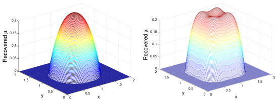
Figure 1. Recovered $\mu$ at Day 1, after 6 h (left), and at Day 2 after 8 h (right), Example 4.

The center-symmetric pictures in Figure 2, Figure 3 and Figure 4 show the spatial density of uncontaminated bees obtained by the inverse problem. Over the first two days, uncontaminated bees are progressively moving away from the hive. This behavior and location pattern matches the one presented in [13]. The regions with different density are smoother, since we study only the contamination-free phenomenon, and as a result we consider a simpler model in comparison with [13].

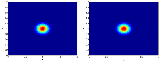
Figure 2. Recovered bee density at Day 1 after 2 h (left), Day 2 after 2 h (right), Example 4.

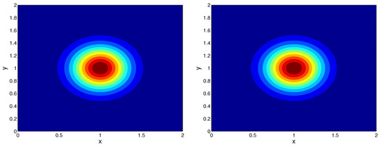
Figure 3. Recovered bee density at Day 1 after 6 h (left), Day 2 after 6 h (right), Example 4.

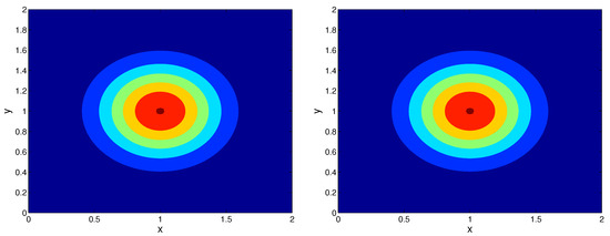
Figure 4. Recovered bee density at Day 1 after 8 h (left), Day 2 after 8 h (right), Example 4.

In Figure 5, the decreasing value of the norm (29) at each iteration is illustrated.

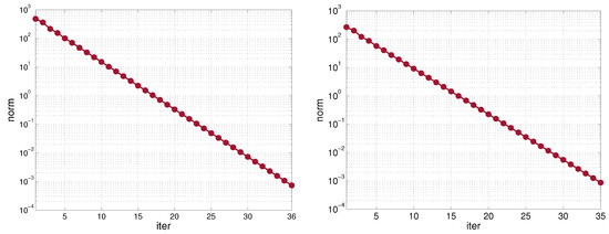
Figure 5. Values of the norm (29) at each iteration at Day 1 after 6 h (left), Day 2 after 6 h (right), Example 4.

7. Conclusions

In this paper, we presented a numerical analysis of forager bee looses in a spatial environment without contamination. The approach was based on the inverse problem for recovering the mortality rate in a honeybee difference equation model that describes forages leaving and entering the hive each day. The mathematical formulation of this process lead to the study of the reaction coefficient identification on the base of final time measurements of the forage bee concentration. After introducing a new solution variable, we reduced the inverse problem to a forward one with a non-local difference operator and a non-local initial condition. For the numerical solution of the problem, different time-stepping techniques were applied to the ODEs system, resulting from second-order difference approximation.

We illustrated, by numerical tests, that for exact measurements, the order of convergence of the solution of the inverse problem for all three methods is the same as in the underlying methods. In the case of perturbed measurements, the most efficient was the iterative approach based on implicit time-stepping. We also observed that in order to achieve good accuracy of the recovered solution, the larger the deviation, the smaller the time step size should be.

The simulations with real data illustrate that the solution of the inverse problem successfully recovers the bee density and the mortality rate of the forage bees and produces relevant results.

In our forthcoming work, we plan to propose a numerical method for solving the inverse problem for a spatial model describing the collapse of honey bee colonies caused by the contamination of foraging bees with pesticides.

References

- Bagheri, S.; Mirzaie, M. A mathematical model of honey bee colony dynamics to predict the effect of pollen on colony failure. PLoS ONE 2019, 14, e0225632. [Google Scholar] [CrossRef]
- Chen, J.; DeGrandi-Hoffman, G.; Ratti, V.; Kang, Y. Review on mathematical modeling of honeybee population dynamics. J. Math. Biosci. Eng. 2021, 18, 9606–9650. [Google Scholar] [CrossRef]
- Van Dooremalen, C.; Gerritsen, L.; Cornelissen, B.; van der Steen, J.J.; van Langevelde, F.; Blacquiere, T. Winter survival of individual honey bees and honey bee colonies depends on level of varroa destructor infestation. PLoS ONE 2012, 7, e36285. [Google Scholar] [CrossRef]
- Fisher, A., II; DeGrandi-Hoffman, G.; Smith, B.H.; Johnson, M.; Kaftanoglu, O.; Cogley, T.; Fewell, J.H.; Harrison, J.F. Colony field test reveals dramatically higher toxicity of a widely-used mito-toxic fungicide on honey bees (apis mellifera). Environ. Pollut. 2021, 269, 115964. [Google Scholar] [CrossRef]
- Genersch, E. American foulbrood in honeybees and its causative agent, paenibacillus larvae. J. Invertebr. Pathol. 2010, 103, S10–S19. [Google Scholar] [CrossRef]
- Laomettachit, T.; Liangruksa, M.; Termsaithong, T.; Tangthanawatsakul, A.; Duangphakdee, O. A model of infection in honeybee colonies with social immunity. PLoS ONE 2021, 16, e0247294. [Google Scholar] [CrossRef]
- Mayack, C.; Naug, D. Energetic stress in the honeybee apis mellifera from nosema ceranae infection. J. Invertebr. Pathol. 2009, 100, 185–188. [Google Scholar] [CrossRef]
- Paris, L.; El Alaoui, H.; Delbac, F.; Diogon, M. Effects of the gut parasite nosema ceranae on honey bee physiology and behavior. Curr. Opin. Insect Sci. 2018, 26, 149–154. [Google Scholar] [CrossRef]
- Smith, K.M.; Loh, E.H.; Rostal, M.K.; Zambrana-Torrelio, C.M.; Mendiola, L.; Daszak, P. Pathogens, pests, and economics: Drivers of honey bee colony declines and losses. Ecohealth 2013, 10, 434–445. [Google Scholar] [CrossRef]
- Williams, B.A. Unique physiology of host-parasite interactions in microsporidia infections. Cell. Microbiol. 2009, 11, 1551–1560. [Google Scholar] [CrossRef]
- DeGrandi-Hoffman, G.; Roth, S.A.; Loper, G.; Erickson, E., Jr. Beepop: A honeybee population dynamics simulation model. Ecol. Modell. 1989, 45, 133–150. [Google Scholar] [CrossRef]
- Becher, M.A.; Osborne, J.L.; Thorbek, P.; Kennedy, P.J.; Grimm, V. Towards a systems approach for understanding honeybee decline: A stocktaking and synthesis of existing models. J. Appl. Ecol. 2013, 50, 868–880. [Google Scholar] [CrossRef]
- Magal, P.; Webb, G.F. A spatial model of honeybee colony collapse due to pesticide contamination of foraging bees. J. Math. Biol. 2020, 80, 2363–2393. [Google Scholar] [CrossRef]
- Bastaansen, R.; Doelman, A.; van Langevede, F.; Rottschafer, V. Modeling honey bee colonies in winter using a Keller-Segel model with a sign-changing chemotectic coefficient. SIAM J. Appl. Math. 2020, 80, 839–863. [Google Scholar] [CrossRef]
- Watmough, J.; Camazine, S. Self-organized thermoregulation of honeybee clusters. J. Theor. Biol. 1995, 176, 391–402. [Google Scholar] [CrossRef]
- Kribs-Zaleta, C.M.; Mitchell, C. Modeling colony collapse disorder in honeybees as a contagion. Math. Biosci. Engn. 2014, 11, 1275–1294. [Google Scholar] [CrossRef]
- Romero-Leiton, J.P.; Gutierrez, A.; Benavides, I.F.; Molina, O.E.; Pulgarin, A. An approach to the modeling of honey bee colonies. Web Ecol. 2022, 22, 7–19. [Google Scholar] [CrossRef]
- Atanasov, A.Z.; Koleva, M.N.; Vulkov, L.G. Numerical analysis of thermoregulation in honey bee colonies in winter based on sign-changing chemotactic coefficient model. In International Conference on New Trends in the Applications of Differential Equations in Sciences; Springer Proceedings in Mathematics & Statistics; Springer: Cham, Switzerland, 2023; Volume 4122, pp. 69–279. [Google Scholar]
- Chavent, G. Nonlinear Least Squares Problems: Theoretical Foundation and Step-by Guide for Applications; Springer: Cham, Switzerland, 2009. [Google Scholar]
- Hasanov, A.H.; Romanov, V.G. Introduction to Inverse Problems for Differential Equations, 1st ed.; Springer: Cham, Switzerland, 2017; 261p. [Google Scholar]
- Isakov, V. Inverse Problems for Partial Differential Equations, 3rd ed.; Springer: Cham, Switzerland, 2017; p. 406. [Google Scholar]
- Ivanov, V.K.; Vasin, V.V.; Tanana, V.P. Theory of Linear Ill-Posed Problems and Its Approximations; Walter de Gruyter: Nauka, Moscow, 1978. (In Russian) [Google Scholar]
- Kabanikhin, S.I. Inverse and Ill-Posed Problems; DeGruyer: Berlin, Germany, 2011. [Google Scholar]
- Lesnic, D. Inverse Problems with Applications in Science and Engineering; CRC Press: Abingdon, UK, 2021; p. 349. [Google Scholar]
- Prilepko, A.I.; Orlovsky, D.G.; Vasin, I.A. Methods for Solving Inverse Problems in Mathematical Physics; Marcel Dekker: New York, NY, USA, 2000. [Google Scholar]
- Prilepko, A.I.; Kostin, A.B.; Solov’ev, V.V. Inverse source and coefficient problems for elliptic and parabolic equations in Hölder and Sobolev spaces. J. Math. Sci. 2019, 237, 576–594. [Google Scholar] [CrossRef]
- Romanov, V.G.; Hasanov, A.H. Uniquiness and stability analysis of final data inverse source problems for evolution equations. J. Inverse Ill-Posed Probl. 2022, 30, 425–446. [Google Scholar] [CrossRef]
- Cao, K.; Lesnic, D. Reconstruction of the perfusion coefficient from temperature measurements using the conjugate gradient method. Int. J. Comput. Math. 2018, 95, 797–814. [Google Scholar] [CrossRef]
- Atanasov, A.; Georgiev, S.; Vulkov, L. Reconstruction analysis of honeybee colony collapse disorder modeling. Optim. Eng. 2021, 22, 2481–2503. [Google Scholar] [CrossRef]
- Atanasov, A.Z.; Georgiev, S.G.; Vulkov, L.G. Parameter Estimation Analysis in a Model of Honey Production. Axioms 2023, 12, 214. [Google Scholar] [CrossRef]
- Atanasov, A.Z.; Koleva, M.N.; Vulkov, L.G. Numerical optimization identification of a Keller-Segel model for thermoregulation in honey bee colonies in winter. Model. Dev. Intell. Syst. Commun. Comput. Inf. Sci. 2023, 1761, 279–293. [Google Scholar]
- Atanasov, A.Z.; Koleva, M.N.; Vulkov, L.G. Parameter estimation inspired by temperature measurements for a chemotactic model of honeybee thermoregulation. In International Conference on Numerical Methods and Applications; Lecture Notes in Computer Science; Springer: Cham, Switzerland, 2023; Volume 13858, pp. 36–47. [Google Scholar]
- Koleva, M.; Vulkov, L. Reconstruction coefficient analysis of honeybee collapse due to pesticide contamination. J. Phys. Conf. Proc. 2023. accepted. [Google Scholar]
- Martin-Vaquero, J.; Sajvicius, S. The two level finite difference scheme for the heat equation with nonlocal initial condition. Appl. Math. Comput. 2019, 342, 160–177. [Google Scholar] [CrossRef]
- Cong, C.; Li, D.; Li, L.; Zhao, D. Crank-Nicolson compact difference scheme for a class of nonlocal nonlinear parabolic problems. Comput. Math. Appl. 2023, 132, 1–17. [Google Scholar]
- Dehghan, M. Numerical schemes for one-dimensional parabolic equations with nonstandard initial condition. Appl. Math. Comput. 2004, 147, 321–331. [Google Scholar] [CrossRef]
- Dehghan, M. Implicit collocation technique for heat equation with non-classic initial condition. Int. J. Nonlinear Sci. Numer. Simul. 2006, 7, 461–466. [Google Scholar] [CrossRef]
- Lin, Y. Analytical and numerical solutions for a class nonlocal nonlinear parabolic differential equations. SIAM J. Math. Anal. 1994, 25, 1577–1594. [Google Scholar] [CrossRef]
- Lin, Y. Finite-difference solutions for parabolic equations with time weighting initial conditions. Appl. Math. Comput. 1994, 65, 49–61. [Google Scholar] [CrossRef]
- Magal, P.; Webb, G.F.; Wu, Y. Environmental model of honey bee colony collapse due to pesticide contamination. Bull. Math. Biol. 2019, 81, 4908–4931. [Google Scholar] [CrossRef] [PubMed]
- Ratti, V.; Kevan, P.G.; Eberl, H.J. A mathematical model of forager loss in honeybee colonies infested with Varroa destructor and accute bee paralysis virus. Bull. Math. Biol. 2017, 79, 1218–1253. [Google Scholar] [CrossRef] [PubMed]
- Il’in, A.M. Differencing Scheme for a differential equation with a small parameter affecting the highest derivative. Mat. Zametki 1969, 6, 237–248. [Google Scholar] [CrossRef]
- Dehghan, M. Three-level techniques for one-dimensional parabolic equation with nonlinear initial condition. Appl. Math. Comput. 2004, 151, 567–579. [Google Scholar] [CrossRef]
- Askar, A.H.; Omle, I.; Kovács, E.; Majár, J. Testing some different implementations of heat convection and radiation in the Leapfrog-Hopscotch algorithm. Algorithms 2022, 15, 400. [Google Scholar] [CrossRef]
- Jalghaf, H.K.; Kovács, E.; Majár, J.; Nagy, Á.; Askar, A.H. Explicit stable finite difference methods for diffusion-reaction type equations. Mathematics 2021, 9, 3308. [Google Scholar] [CrossRef]
- Nagy, Á.; Omle, I.; Kareem, H.; Kovacs, E.; Barna, I.F.; Bognar, G. Stable, Explicit, Leapfrog-Hopscotch Algorithms for the Diffusion Equation. Computation 2021, 9, 92. [Google Scholar] [CrossRef]
- Saleh, M.; Kovács, E.; Barna, I.F.; Mátyás, L. New analytical results and comparison of 14 numerical schemes for the diffusion equation with space-dependent diffusion coefficient. Mathematics 2022, 10, 2813. [Google Scholar] [CrossRef]
- Samarskii, A.A.; Vabishchevich, P.N. Numerical Methods for Solving Inverse Problems in Mathematical Physics; de Gruyter: Berlin, Germany, 2007; 438p. [Google Scholar]
Disclaimer/Publisher’s Note: The statements, opinions and data contained in all publications are solely those of the individual author(s) and contributor(s) and not of MDPI and/or the editor(s). MDPI and/or the editor(s) disclaim responsibility for any injury to people or property resulting from any ideas, methods, instructions or products referred to in the content. |
© 2023 by the authors. Licensee MDPI, Basel, Switzerland. This article is an open access article distributed under the terms and conditions of the Creative Commons Attribution (CC BY) license (https://creativecommons.org/licenses/by/4.0/).