Alternative Derivation of the Non-Abelian Stokes Theorem in Two Dimensions

Abstract

The relation between the holonomy along a loop with the curvature form is a well-known fact, where the small square loop approximation of aholonomy $\mathit{H}\left(\gamma ,\mathcal{O}\right)$ is proportional to $\mathit{R}\left(\sigma \right)$. In an attempt to generalize the relation for arbitrary loops, we encounter the following ambiguity. For a given loop $\gamma$ embedded in a manifold $\mathcal{M}$, $\mathit{H}\left(\gamma ,\mathcal{O}\right)$ is an element of a Lie group $\mathcal{G}$; the curvature $\mathit{R}\left(\sigma \right)\in \mathfrak{g}$ is an element of the Lie algebra of $\mathcal{G}$. However, it turns out that the curvature form $\mathit{R}\left(\sigma \right)$ obtained from the small loop approximation is ambiguous, as the information of $\gamma$ and $\mathit{H}\left(\gamma ,\mathcal{O}\right)$ are insufficient for determining a specific plane $\sigma$ responsible for $\mathit{R}\left(\sigma \right)$. To resolve this ambiguity, it is necessary to specify the surface $\mathcal{S}$ enclosed by the loop $\gamma$; hence, $\sigma$ is defined as the limit of $\mathcal{S}$ when $\gamma$ shrinks to a point. In this article, we try to understand this problem more clearly. As a result, we obtain an exact relation between the holonomy along a loop with the integral of the curvature form over a surface that it encloses. The derivation of this result can be viewed as an alternative proof of the non-Abelian Stokes theorem in two dimensions with some generalizations.

1. Introduction

The intrinsic curvature of the connection on a manifold can be expressed in various manners; one of the standard expressions is the curvature 2-form, which measures the intrinsic curvature of a connection on a manifold at a single point in the direction of a given bivector. The measurement of intrinsic curvature via the curvature form at a point is regarded as a local infinitesimal measurement. However, to a certain extent there is a need for a notion of curvature defined in a finite non-local region, in the sense that the curvature is associated with an object containing more than a single point of the manifold. A good example of subjects where this notion is frequently used is discrete geometry and its applications. One of the objects able to capture the curvature in a finite non-local region is the holonomy, which is an element of a Lie group attached to an arbitrary curve on the manifold. It captures the curvature of the connection on the manifold by measuring the difference between the final and initial tangent vectors transported in parallel along a curve. For the holonomy on a closed curve, it is possible to classify the corresponding Lie group into special subgroups based on the types of the manifolds and their corresponding connections; see [1,2,3].

It is a well-known fact that the holonomy group is related to the curvature 2-form. The work by Ambrose and Singer in [4] contains a proof that the holonomy group $\mathrm{Hol}(\mathcal{M},\mathcal{O})\subset \mathcal{G}$, with $\mathcal{G}$ is a Lie group generated by the curvature of the connection $\mathfrak{hol}\subset \mathfrak{g}$, with $\mathfrak{g}$ being the Lie algebra of $\mathcal{G}$. This result is widely used in mathematical physics subjects, mainly as an approximation of the calculation of holonomy along small loops, as well as to provide a link between the continuous theory of smooth differential geometry and its discrete counterpart. However, it can be observed that there is an ambiguity in the relation between the non-local finite holonomy and the local curvature form; this becomes apparent only when one considers the small loop limit, that is, when the loop shrinks to a point. One of the objectives of this article is to clarify this ambiguity using pre-existing concepts as the solution to the problem, as well as to obtain an exact and approximation formula between the non-local finite holonomy and the local curvature form.

We present the ambiguity as follows. Consider a tangent bundle $T\mathcal{M}={\bigcup }_p\left\{p\right\}\times T_p\mathcal{M},$ with $\left(\mathcal{M},g,\nabla \right)$ as an oriented manifold equipped with a metric g and an affine connection ∇, where its value lies in $\mathfrak{g}$. Here, ∇ is not necessarily Levi-Civita, and the curvature form of the connection ∇, $\mathit{R}\left(..,..\right)$ is defined on each point of the manifold. It acts on two vectors $U,V\in T_p\mathcal{M}$ to provide a Lie algebra element $\mathit{R}\left(U,V\right)\in \mathfrak{g}$. For a given (not necessarily smooth) loop $\gamma$ embedded in $\mathcal{M}$ with an origin point $\mathcal{O}$, we can obtain the corresponding holonomy $\mathit{H}\left(\gamma ,\mathcal{O}\right)$ on the loop. For a manifold with a dimension larger than 2, it is possible to construct infinitely many continuous (not necessarily smooth) surfaces $\mathcal{S}$ such that they are enclosed by the loop $\gamma =\partial \mathcal{S}$ as the boundary of $\mathcal{S}$. The non-uniqueness of $\mathcal{S}$ with respect to the boundary does not become a problem for the holonomy, as it does not depend on the surface, only on the variables on the loop. However, a problem appears if we consider the infinitesimal limit under the condition that the loop shrinks to a point. As the loop shrinks, the holonomy (which is an element of a Lie group) changes accordingly, and at the shrinking point it is approximated by the Lie algebra element derived from the curvature form $\mathit{R}\left(U,V\right)$. To obtain a specific Lie algebra from the local curvature form, $\mathit{R}\left(..,..\right)$ needs to act on a specific plane, which in this case is defined by the wedge product of two vectors $U,V\in T_p\mathcal{M}$. How is it possible to obtain the plane $U\wedge V$ with only the information of the finite loop $\gamma$ and the finite holonomy $\mathit{H}\left(\gamma ,\mathcal{O}\right)$ on $\left(\mathcal{M},g\right)$? It has been mentioned in a number of works that the plane is an approximation of the surface enclosed by the small loop; however, as we have mentioned previously, there exist infinitely many possible surfaces enclosed by the loop. Elsewhere in the literature, it has been argued that the small loop encloses a flat Euclidean plane, which is similarly not well-defined, as the loop may not always be embedded in a flat plane.

It turns out that the solution to the ambiguity presented earlier is to consider a finite loop together with a contraction procedure. It can be observed that, with only the information of a finite loop and its holonomy, different contraction procedures could result in a different infinitesimal loop and different Lie algebra element at the shrinking point. Hence, by providing a specific contraction procedure together with a finite loop $\gamma$ and the holonomy $\mathit{H}\left(\gamma ,\mathcal{O}\right)$ in the non-local finite setting, we are led to a specific Lie algebra element when the loop shrinks to a point, which comes from the action of the curvature form $\mathit{R}\left(..,..\right)$ on a specific plane $\sigma =U\wedge V\in T_p^2\mathcal{M}$. The loop contraction procedure is realized by defining a specific homotopy acting on the loop $\gamma$; such a choice of homotopy exactly singles out a (homotopic) surface $\mathcal{S}$ from infinitely many possible choices. The concept of homotopy has already been considered, and was used to prove the main theorem in [4].

As the main result in this article, we prove for any arbitrary loop an exact relation between a non-local finite holonomy $\mathit{H}\left(\gamma ,\mathcal{O}\right)={\mathit{H}}_{\gamma \left[0,1\right]}$ of a general affine connection, with the integral of the curvature $\mathit{R}\left(..,..\right)$ over a specific surface $\mathcal{S}$ with a boundary $\gamma$, as follows:

$${\mathit{H}}_{\gamma \left[0,1\right]}={\widehat{P}}_{\gamma }exp-\underset{\mathcal{S}}{\int }\overline{\mathit{R}},$$

(1)

where $\overline{\mathit{R}}$, widely known as the twisted curvature, is the conjugation of the curvature form $\mathit{R}$ by an element of group $\mathcal{G}$. This is already a well-known result, and has been studied extensively under the heading of the non-Abelian Stokes theorem; for examples, see [5,6,7,8]. However, the derivation carried out in this article differs from those found in the existing literature, and contains several generalizations. Hence, our work can be viewed as an alternative proof of the non-Abelian Stokes theorem for 2D surfaces.

The rest of this article is organized as follows. Section 2.1 contains the standard definition of the curvature 2-form, starting with the definition of the affine connection on $\mathcal{M}$. We introduce new terminologies to complement those in [9]. Section 2.2 contains the precise definition of parallel transport and holonomy. In Section 3.1, we present the ambiguity concerning the infinitesimal holonomy in a more detailed manner using the new terminology introduced previously. A clarification via introduction of the homotopy is presented here as well. Prior to the proof of Equation (1), we obtain an important relation, namely, the near-zero approximation of the holonomy along a loop. As a corollary of this relation, we prove the non-Abelian Stokes theorem for two-dimensional surfaces in Section 3.2. In Section 3.3, we prove Equation (1) using the near-zero approximation and present it as a theorem. We provide additional commentary on the non-Abelian Stokes theorem, together with generalizations presented in our work. In the last section, we discuss a number of relevant subtleties and discuss how the relation in (1) clarifies the ambiguity mentioned earlier in Section 4.1, then finally conclude our work in Section 4.2.

2. The Curvature 2-Form and Holonomy

2.1. Local Intrinsic Curvature: The Curvature 2-Form

For a given a tangent bundle $T\mathcal{M}={\bigcup }_p\left\{p\right\}\times T_p\mathcal{M}$ with $\left(\mathcal{M},g\right)$ being an oriented (continuous, differentiable) manifold equipped with a metric g, it is possible to construct an affine connection acting on an element of tangent space $U\in T_p\mathcal{M}$ as follows:

$$\begin{array}{cc}\hfill {\nabla }_U:T_p\mathcal{M}& \to T_{p+\Delta p}\mathcal{M},\Delta p\to 0,\hfill \\ \hfill X& \mapsto {\nabla }_{U}X=U^{\mu }\left({\partial }_{\mu }X+{\omega }_{\mu }\left(X\right)\right).\hfill \end{array}$$

(2)

where $\omega ={\omega }_{\mu }d{x}^{\mu }$ is the vector potential, which is a matrix-valued 1-form where the value lies in a (representation of) the Lie algebra $\mathfrak{g}$ of a Lie group $\mathcal{G}$. The connection ∇ is usually known as the covariant derivative.

The curvature form of a connection is a tensor of order $\left(\genfrac{}{}{0pt}{}{1}{3}\right)$: $\mathit{R}\left(..,..\right)=R_{\mu \nu \beta }^{\alpha }\left(d{x}^{\mu }\otimes d{x}^{\nu }\right)\times \left({\partial }_{\alpha }\otimes d{x}^{\beta }\right).$ It associates two tangential vectors to an element of the (representation of) $\mathfrak{g}$:

$$\begin{array}{ccc}\hfill \mathit{R}\left(..,..\right):T_p\mathcal{M}\times T_p\mathcal{M}& \to & \mathfrak{g},\hfill \\ \hfill U,V& \mapsto & \mathit{R}\left(U,V\right)=\left(U^{\mu }{V}^{\nu }{R}_{\mu \nu \beta }^{\alpha }\right){\partial }_{\alpha }\otimes d{x}^{\beta },\hfill \end{array}$$

(3)

which in turns acts on an element of the tangent space $X\in T_p\mathcal{M}$ as follows:

$$\begin{array}{ccc}\hfill \mathit{R}\left(U,V\right):T_p\mathcal{M}& \to & T_p\mathcal{M},\hfill \\ \hfill X& \mapsto & \mathit{R}\left(U,V\right)X=\left(U^{\mu }{V}^{\nu }{R}_{\mu \nu \beta }^{\alpha }{X}^{\beta }\right){\partial }_{\alpha }\otimes d{x}^{\beta },\hfill \end{array}$$

(4)

where

$$\mathit{R}\left(U,V\right)X=\left[{\nabla }_U,{\nabla }_V\right]X-{\nabla }_{\left[U,V\right]}X.$$

(5)

For the Levi-Civita connection, (5) is the standard definition of the Riemann tensor.

The curvature form satisfies a specific symmetry:

$$\mathit{R}\left(U,V\right)=-\mathit{R}\left(V,U\right),U,V\in T_p\mathcal{M},$$

(6)

which is a direct consequence of definition (5). The symmetry has the following geometrical interpretation: for a given test vector $X\in T_p\mathcal{M}$, the quantity $\mathit{R}\left(U,V\right)X$ measures the difference between the original and the parallel-transported test vector, carried along an infinitesimal parallelogram composed by the infinitesimal line U and V: $\mathit{R}\left(U,V\right)X=\Delta X=X^{\prime }-X$.

A general transformation $\Lambda$ is generated by a generator $d\Lambda$ such that the infinitesimal transformation acting on an element of the representation space is $x^{\prime }=x+\Delta x\approx \left(\mathbb{I}+d\Lambda \right)x$, with $\mathbb{I}$ being an identity and the generator $d\Lambda$ being an element of the Lie algebra $\mathfrak{g}$ if the transformation is an element of a Lie group $\mathcal{G}$. In this sense, $\mathit{R}\left(U,V\right)\in \mathfrak{g}$ is a generator of a group transformation:

$$X^{\prime }=X+\Delta X\approx \left(\mathbb{I}-\mathit{R}\left(U,V\right)\right)X=\mathit{h}(U,V)X,$$

(7)

with X as a test vector and $\mathit{h}(U,V)$ as the infinitesimal group transformation, called the local holonomy. Here, $\mathit{h}(U,V)$ is generated by $\mathit{R}\left(U,V\right)$, and is associated with a plane defined by $U,V$. In fact, all elements of the holonomy group (say, the subgroup $\mathrm{Hol}\subset \mathcal{G}$) are generated by the curvature of the connection (and exactly define the subalgebra $\mathfrak{hol}\subset \mathfrak{g}$ of $\mathrm{Hol}$), as proven in the Ambrose–Singer holonomy theorem [4].

The curvature form components $R_{\mu \nu \beta }^{\alpha }$ are antisymmetric in the indices $\left(\mu ,\nu \right)$ due to the condition (6). The $\left(\mu ,\nu \right)$-indices of $\mathit{R}$ label the components of the infinitesimal loop orientation, while the $\left(\alpha ,\beta \right)$-indices label the components of the ‘rotation bivector’ [9] (the term ‘rotation bivector’, introduced in [9], was originally used for a Levi-Civita connection, where ${\mathit{R}}_{\mu \nu }\in \mathfrak{g}=\mathfrak{o}\left(\mathfrak{n}\right)$. In this article, we adopt a similar term; however, $\mathfrak{g}$ is not necessarily $\mathfrak{o}\left(\mathfrak{n}\right)$. It needs to be kept in mind that the notion of orthogonality is defined with respect to the metric g). For each component of the infinitesimal loop orientation, there is a corresponding rotation bivector attached.

From map (3), the definition of the curvature form requires that the argument of $\mathit{R}\left(..,..\right)$ consist of two vectors $U,V$ such that the rotation bivector is defined by $\mathit{R}\left(U,V\right)=U^{\mu }{V}^{\nu }{\mathit{R}}_{\mu \nu }$. In fact, from the symmetry (6), we can generalize the definition such that the argument of $\mathit{R}\left(..,..\right)$ is a plane $\sigma$, that is, the map becomes

$$\begin{array}{cc}\hfill \mathit{R}\left(..,..\right):\stackrel{2}{\bigwedge }\left(\mathcal{M}\right)& \to \mathfrak{g}\hfill \\ \hfill \sigma & \mapsto \mathit{R}\left(\sigma \right),\hfill \end{array}$$

(8)

where $\sigma$ is now an element of the bivector space over $\mathcal{M}$.

Written in the form of (8), the curvature is a linear operator on the argument, and satisfies

$$\mathit{R}\left(c_1{\sigma }_1+c_2{\sigma }_2\right)=c_1\mathit{R}\left({\sigma }_1\right)+c_2\mathit{R}\left({\sigma }_2\right),$$

(9)

with $c_1,c_2\in \mathbb{R}$ and ${\sigma }_1,{\sigma }_2\in {\bigwedge }^2\left(\mathcal{M}\right).$ Notice that it is not possible to have this nice linear property for both vector arguments simultaneously in the standard formulation (3), as they are linear only on each of the arguments. The corresponding infinitesimal transformation of $\mathit{R}\left(\sigma \right)$, as in (7), is $\mathit{h}\left(\sigma \right)$:

$$X^{\prime }=X+\Delta X\approx \left(\mathbb{I}+\mathit{R}\left(\sigma \right)\right)X=\mathit{h}\left(\sigma \right)X,$$

(10)

which is associated with the bivector $\sigma$.

In addition to the terminologies introduced in [9], we add another term. The (simple) bivector $\sigma$ in (8) is termed the evaluation plane. From (3), it is clear that the loop orientation ${\mathit{R}}_{\mu \nu }d{x}^{\mu }\otimes d{x}^{\nu }$ acts on the evaluation plane $\sigma$ such that it provides ${\sigma }^{\mu \nu }{\mathit{R}}_{\mu \nu }$ (with hidden indices $\alpha ,\beta$); this is the rotation bivector projected in the direction $\sigma$. Hence, we have three bivectors for the curvature form; two of them, namely, the infinitesimal loop orientation and the rotation bivector, are the properties intrinsic to the curvature map, while the later, which is the evaluation plane, depends on the direction chosen to evaluate the curvature form at a point.

2.2. Non-Local Intrinsic Curvature: Holonomy

As a finite generalization of the local flat evaluation plane, we can define the non-local finite evaluation surface. In analogy to the evaluation plane $\sigma$, the evaluation surface is defined by an embedded surface with boundary $\mathcal{S}\subset \mathcal{M}$, with a loop $\gamma =\partial \mathcal{S}$ acting as its boundary. The evaluation plane is associated with the Lie algebra originating from the curvature of a connection $\mathit{R}\left(\sigma \right)$ (or, equivalently, an infinitesimal transformation $\mathit{h}\left(\sigma \right)=1+\mathit{R}\left(\sigma \right)$) along an infinitesimal loop enclosing the plane $\sigma$. With a similar analogy, along the loop $\gamma =\gamma \left(\lambda \right)$ (with a real parameter $\lambda$) as the boundary of the finite evaluation surface $\mathcal{S}$ we have a finite transformation such that a test vector $X\left[\gamma \left(0\right)\right]\in T_{\mathcal{O}}\mathcal{M}$ parallel-transported along $\gamma$ satisfies

$$X\left[\gamma \left(\lambda \right)\right]=\mathit{H}\left(\gamma ,\mathcal{O}\right)X\left[\gamma \left(0\right)\right].$$

(11)

The finite transformation $\mathit{H}\left(\gamma ,\mathcal{O}\right)$ is known as the holonomy along loop $\gamma$ with origin $\mathcal{O}.$ In fact, the holonomy is derived from the solution to a parallel-transport equation along a curve $\gamma$ (not necessarily closed), namely,

$${\nabla }_{\dot{\gamma }\left(\lambda \right)}X\left[\gamma \left(\lambda \right)\right]=0,$$

(12)

with $\dot{\gamma }\left(\lambda \right)=\frac{d\gamma }{d\lambda }$ sending the test vector $X\left[\gamma \left(0\right)\right]$ into a transformed vector $X\left[\gamma \left(\lambda \right)\right]$, as in (11). We obtain $\mathit{H}\left(\gamma ,\mathcal{O}\right)$ by solving (12) in a recursive manner:

$$\mathit{H}\left(\gamma ,\mathcal{O}\right)={\widehat{P}}_{\gamma }exp-\underset{\gamma }{\int }\omega .$$

(13)

Notice that if we replace the vector $X\in T_{\mathcal{O}}\mathcal{M}$ with a covector $\alpha \in T_{\mathcal{O}}^{*}\mathcal{M}$, then a plus sign is obtained in front of the exponential in (13). Here, $\omega$ is the (vector potential of the) connection on $\mathcal{M}$ and ${\widehat{P}}_{\gamma }$ is the path-ordered operator acting on the integral of the connection along $\gamma$ such that

$$\frac{{\widehat{P}}_{\gamma }}{n!}{\left(\underset{\gamma }{\int }\omega \right)}^n=\underset{0}{\overset{1}{\int }}\cdots \underset{{\lambda }_n=0}{\overset{{\lambda }_n={\lambda }_{n+1}}{\int }}\cdots \underset{{\lambda }_2=0}{\overset{{\lambda }_2={\lambda }_3}{\int }}\underset{{\lambda }_1=0}{\overset{{\lambda }_1={\lambda }_2}{\int }}\omega \left({\lambda }_n\right)\cdots \omega \left({\lambda }_1\right),1\ge \cdots \ge {\lambda }_n\cdots \ge {\lambda }_2\ge {\lambda }_1\ge 0.$$

(14)

This permits a continuous-piecewise property of the holonomy; for a give curve decomposable into two curves ${\gamma }_{12}={\gamma }_2\circ {\gamma }_1$, the holonomy along $\gamma$ is a product between the holonomies on each curve: $\mathit{H}\left({\gamma }_{12},\mathcal{O}\right)X=\mathit{H}\left({\gamma }_2,{\gamma }_1\left(1\right)\right)\mathit{H}\left({\gamma }_1,\mathcal{O}\right)X.$ The end of curve ${\gamma }_1\left(\lambda \right)$ is the origin of curve ${\gamma }_2\left(\lambda \right)$, that is, ${\gamma }_1\left(1\right)={\gamma }_2\left(0\right)$, with $0\le \lambda \le 1$ being a real parameter for the curves. By expanding the exponential, (13) can be written as the following Dyson power series:

$$\begin{array}{cc}\hfill \mathit{H}\left(\gamma ,\mathcal{O}\right)={\widehat{P}}_{\gamma }\sum _{n=0}^{\infty }\frac{{\left(-1\right)}^n}{n!}{\left(\underset{\gamma }{\int }\omega \right)}^n& =\mathbb{I}-\underset{0}{\overset{1}{\int }}\omega \left(\lambda \right)d\lambda +\underset{0}{\overset{1}{\int }}\underset{{\lambda }_1=0}{\overset{{\lambda }_1={\lambda }_2}{\int }}\omega \left({\lambda }_2\right)\omega \left({\lambda }_1\right)d{\lambda }_{1}d{\lambda }_2\hfill \\ \hfill & -\underset{0}{\overset{1}{\int }}\underset{{\lambda }_2=0}{\overset{{\lambda }_2={\lambda }_3}{\int }}\underset{{\lambda }_1=0}{\overset{{\lambda }_1={\lambda }_2}{\int }}\omega \left({\lambda }_3\right)\omega \left({\lambda }_2\right)\omega \left({\lambda }_1\right)d{\lambda }_{1}d{\lambda }_{2}d{\lambda }_3+\cdots ,\hfill \end{array}$$

(15)

with $1\ge \cdots \ge {\lambda }_1\ge 0$, where we use the definition in (14).

In this article, we are particularly interested in the case of holonomies along closed curves. The holonomy along a loop $\gamma$ of a connection $\omega$ is an element of a group $\mathcal{G}$:

$$\mathit{H}\left(\gamma ,\mathcal{O}\right)={\widehat{P}}_{\gamma }exp-\underset{\gamma }{\oint }\omega .$$

(16)

3. Relation between Holonomy and Curvature Form

3.1. Loop Contraction, Homotopy, and Evaluation Surface

The relation between the holonomy along a finite non-local loop $\gamma$, $\mathit{H}\left(\gamma ,\mathcal{O}\right)$, with the Lie algebra element of the curvature form at a local point $\mathit{R}\left(\sigma \right)$, is quite subtle. The reason is due to the fact that the association of $\mathit{R}\left(\sigma \right)$ with $\mathit{H}\left(\gamma ,\mathcal{O}\right)$ is not one-to-one, in the sense that there are infinitely many ways to shrink a loop $\gamma$ to a point $\mathcal{O}$. By defining $\sigma$ as the limit of $\mathcal{S}$ when $\gamma$ shrinks to a point, contracting the loop $\gamma$ along different surfaces results in a different plane $\sigma$ at the origin $\mathcal{O}$. Therefore, to associate a specific $\mathit{R}\left(\sigma \right)$ with $\mathit{H}\left(\gamma ,\mathcal{O}\right)$, it is necessary to specify a loop contraction. This can be done through the concept of homotopy.

Consider the following continuous map:

$$\begin{array}{ccc}\hfill \mathcal{S}:\left[0,1\right]\times I& \to & \mathcal{M},\hfill \\ \hfill \left(\tau ,\lambda \right)& \mapsto & \mathcal{S}\left(\tau ,\lambda \right),\hfill \end{array}$$

(17)

where $I\subset \mathbb{R}$ is a real interval and $\mathcal{S}\left(\tau ,\lambda \right):={\gamma }^{\left(\tau \right)}\left(\lambda \right)$ is defined as a set of curves with one real parameter

$$\begin{array}{cc}\hfill {\gamma }^{\left(\tau \right)}:I& \to \mathcal{M},\hfill \\ \hfill \lambda & \mapsto {\gamma }^{\left(\tau \right)}\left(\lambda \right),\hfill \end{array}$$

(18)

where $\mathcal{S}\left(\tau ,\lambda \right)$ is a homotopy on $\mathcal{M}.$

The next step is to apply the map in (17) to a family of loops in which each element of the family satisfies the following condition:

$${\gamma }^{\left(\tau \right)}\left(0\right)={\gamma }^{\left(\tau \right)}\left(1\right)=\mathcal{O}.$$

(19)

We can specify two loops on $\mathcal{M}$, denoted $\gamma \left(\lambda \right)$ and ${\gamma }^{\prime }\left(\lambda \right)$, that share an identical origin $\mathcal{O}$, with ${\gamma }^{\prime }\left(\lambda \right)=\mathbf{0}$ being an infinitesimal loop (effectively, a point at $\mathcal{O}$ if the origin is at the coordinate $\mathbf{0}$). The loop contraction of $\gamma \left(\lambda \right)$ is defined as the homotopy (17), with an additional requirement such that the following ‘boundary condition’ is satisfied:

$$\begin{array}{cc}\hfill {\gamma }^{\left(1\right)}\left(\lambda \right)=\gamma \left(\lambda \right),{\gamma }^{\left(0\right)}\left(\lambda \right)& ={\gamma }^{\prime }\left(\lambda \right)=\mathbf{0}.\hfill \end{array}$$

(20)

If there exists a homotopy satisfying the conditions, then $\gamma \left(\lambda \right)$ is contractible on $\mathcal{M}$. This provides a well-defined procedure for shrinking an arbitrary loop to a local point. It can be observed that the homotopy is a continuous (though not necessarily smooth) surface embedded on $\mathcal{M}$, specifically, $\mathcal{S}\left(\tau ,\lambda \right)\subset \mathcal{M}$.

The evaluation surface of a loop ${\gamma }^{\left(1\right)}\left(\lambda \right)$ is defined as the homotopy $\mathcal{S}\left(\tau ,\lambda \right):={\gamma }^{\left(\tau \right)}\left(\lambda \right)$ satisfying (19) and (20). Specifying a homotopy, we can single out an evaluation surface $\mathcal{S}\left(\tau ,\lambda \right)$ from the many possible choices of surfaces enclosed by a specific loop ${\gamma }^{\left(1\right)}\left(\lambda \right)$, and thereby solve the corresponding ambiguity.

3.2. Near-Zero Approximation and the Non-Abelian Stokes Theorem

In this section, we derive the near-zero approximation (or near-$\mathcal{O}$ approximation) of the holonomy along an arbitrary loop, then use this approximation to prove the non-Abelian Stokes theorem in two dimensions. This can be easily accomplished by expanding Equation (16) and taking only the first leading-order term, as follows:

$$\underset{\omega \to 0}{lim}\mathit{H}\left(\gamma ,\mathcal{O}\right)=\mathbb{I}-\underset{\gamma }{\int }\omega ,$$

(21)

where we are interested in obtaining the nearly flat relation in terms of the curvature form instead of the connection. Here, we show that relation (21) can be obtained through another approach.

3.2.1. The Generalized Twisted Curvature

Here, it is convenient to review a number of conventions used in this article. The group element $\mathit{H}$ acts on a vector $X_p\in T_p\mathcal{M}$ as a left action $\mathit{H}\left(X_p\right)=\mathit{H}{X}_p$, and acts on the co-vector ${\alpha }_p\in T_p^{*}\mathcal{M}$ as a right action ${\mathit{H}}^{*}\left({\alpha }_p\right)={\alpha }_p{\mathit{H}}^{*}$. A curve $\gamma$ is labeled with ${\gamma }^{\left(\tau \right)}\left[{\lambda }_i,{\lambda }_f\right]$, with $\tau$ as the fixed parameter and where ${\lambda }_i$ and ${\lambda }_f$ are respectively the initial and final single real parameters of the loop. Ensuring a consistent convention is important for the derivation throughout this article.

Let us consider a homotopic surface with a boundary $\mathcal{S}\left(\tau ,\lambda \right)$ satisfying (17)–(19) and the boundary condition (20). It can be written in local coordinates as $\mathcal{S}\left(\tau ,\lambda \right)=x^{\mu }\left(\tau ,\lambda \right).$ A family of loops ${\gamma }^{\left(\tau \right)}\left(\lambda \right)$ defines a specific parameterization of $\mathcal{S}\left(\tau ,\lambda \right)$, as shown in Figure 1a. The boundary of $\mathcal{S}\left(\tau ,\lambda \right)$ is $\partial \mathcal{S}={\gamma }^{\left(1\right)}\left(\lambda \right)$. On each point of $\mathcal{S}\left(\tau ,\lambda \right)$, the curvature form ${\left.\mathit{R}\right|}_{\tau ,\lambda }={\mathit{R}}_{\left(\mathcal{S}\left(\tau ,\lambda \right)\right)}$, which varies according to the coordinate position, is attached; ${\mathit{R}}_{\left(\mathcal{S}\left(\tau ,\lambda \right)\right)}$ can be parallel-transported to the origin $\mathcal{O}$ by the holonomy $\mathit{H}\left(\gamma ,\mathcal{O}\right)=$${\mathit{H}}_{{\gamma }^{\left(\tau \right)}\left(\lambda \right)}$ along a specific loop ${\gamma }^{\left(\tau \right)}\left(\lambda \right)$. We define the quantity as follows:

$${\tilde{\mathit{R}}}_{\left(\mathcal{S}\left(\tau ,\lambda \right)\right)}\left(X_p\right)=\left({\mathit{H}}_{{\gamma }^{\left(\tau \right)}\left[\lambda ,1\right]}{\mathit{R}}_{\left(\mathcal{S}\left(\tau ,\lambda \right)\right)}{\mathit{H}}_{{\gamma }^{\left(\tau \right)}\left[0,\lambda \right]}\right)\left(X_p\right),X_p\in T_p\mathcal{M},$$

(22)

labeled as the (path-dependent) generalized twisted curvature. Equation (22) is a more general version of the standard twisted curvature in [6], which has the form $\overline{\mathit{R}}={\mathit{H}}_{\gamma }^{-1}\mathit{R}{\mathit{H}}_{\gamma }$. In (22), ${\mathit{H}}_{{\gamma }^{\left(\tau \right)}\left[0,\lambda \right]}$ and ${\mathit{H}}_{{\gamma }^{\left(\tau \right)}\left[\lambda ,1\right]}$ are the holonomies along the open curves ${\gamma }^{\left(\tau \right)}\left[0,\lambda \right]$ and ${\gamma }^{\left(\tau \right)}\left[\lambda ,1\right]$, respectively. Notice that these curves define a closed loop by ${\gamma }^{\left(\tau \right)}\left[\lambda ,1\right]\circ {\gamma }^{\left(\tau \right)}\left[0,\lambda \right]={\gamma }^{\left(\tau \right)}\left(\lambda \right)$ and that their holonomies satisfy ${\mathit{H}}_{{\gamma }^{\left(\tau \right)}\left(\lambda \right)}\left(X_p\right)=\left({\mathit{H}}_{{\gamma }^{\left(\tau \right)}\left[\lambda ,1\right]}{\mathit{H}}_{{\gamma }^{\left(\tau \right)}\left[0,\lambda \right]}\right)\left(X_p\right)$; see Figure 1.

Figure 1. (a) A specific parametrization of $\mathcal{S}\left(\tau ,\lambda \right)$ by a family of loops ${\gamma }^{\left(\tau \right)}\left(\lambda \right)$ (black). This illustration describes a circle; in general, though, it could be any arbitrary loop. Each loop is obtained by fixing the parameter $\tau$. (b) Loop ${\gamma }^{\left(\tau \right)}\left(\lambda \right)$ is divided into two open curves at point $\mathcal{S}\left(\tau ,\lambda \right)$, namely, ${\gamma }^{\left(\tau \right)}\left[0,\lambda \right]$ (red) and ${\gamma }^{\left(\tau \right)}\left[\lambda ,1\right]$ (black). A vector $X_p\in T_p\mathcal{M}$ is transported to $T_{\mathcal{S}\left(\tau ,\lambda \right)}\mathcal{M}$ by the curve ${\gamma }^{\left(\tau \right)}\left[0,\lambda \right]$. (c) A covector ${\alpha }_p\in T_p^{*}\mathcal{M}$ is transported to $T_{\mathcal{S}\left(\tau ,\lambda \right)}^{*}\mathcal{M}$ by the curve ${\gamma }^{\left(\tau \right)}\left[1,\lambda \right]={\left({\gamma }^{\left(\tau \right)}\left[\lambda ,1\right]\right)}^{-1}$ (blue). (b,c) Illustration of the geometrical interpretation of relations (43)–(44).

In the following paragraphs, we omit the vector $X_p\in T_p\mathcal{M}$ from the equations concerning the twisted curvature; nonetheless, it is important to keep in mind that (22) is a map acting on vectors.

Let us consider the integral of $\tilde{\mathit{R}}$ over the homotopic surface $\mathcal{S}\left(\tau ,\lambda \right)$, as follows:

$$\underset{\mathcal{S}\left(\tau ,\lambda \right)}{\int }{\tilde{\mathit{R}}}_{\left(\mathcal{S}\left(\tau ,\lambda \right)\right)}=\underset{\mathcal{S}\left(\tau ,\lambda \right)}{\int }{\mathit{H}}_{{\gamma }^{\left(\tau \right)}\left[\lambda ,1\right]}{\mathit{R}}_{\left(\mathcal{S}\left(\tau ,\lambda \right)\right)}{\mathit{H}}_{{\gamma }^{\left(\tau \right)}\left[0,\lambda \right]}.$$

(23)

Considering that the integral in (23) is a Riemann sum, we can observe that the twisted curvature ${\tilde{\mathit{R}}}_{\left(\mathcal{S}\left(\lambda ,\tau \right)\right)}$ satisfying (22) is defined in such a way that we can sum together the local curvature forms on different points over $\mathcal{S}$; hence, these need to be parallel-transported to $\mathcal{O}$ by the holonomies ${\mathit{H}}_{{\gamma }^{\left(\tau \right)}\left[0,\lambda \right]}$ and ${\mathit{H}}_{{\gamma }^{\left(\tau \right)}\left[\lambda ,1\right]}$. Using the wedge product, the curvature form can be written as a matrix (Lie algebra)-valued 2-form:

$$\begin{array}{cc}\hfill {\mathit{R}}_{\left(\mathcal{S}\left(\tau ,\lambda \right)\right)}& ={\left.{\mathit{R}}_{\mu \nu }\right|}_{\mathcal{S}\left(\tau ,\lambda \right)}d{x}^{\mu }\otimes d{x}^{\nu },\mu ,\nu =1,\cdots ,n,\hfill \\ \hfill & ={\left.{\mathit{R}}_{\mu \nu }\right|}_{\mathcal{S}\left(\tau ,\lambda \right)}d{x}^{\mu }\wedge d{x}^{\nu },\mu ,\nu =1,\cdots ,n,\mu <\nu .\hfill \end{array}$$

(24)

Applying a change of coordinate $d{x}^{\mu }=\frac{\partial x^{\mu }}{\partial \tau }d\tau +\frac{\partial x^{\mu }}{\partial \lambda }d\lambda$ to (24), we can obtain the following (with the interval $I\ni \lambda$ going from 0 to 1):

$$\underset{\mathcal{S}\left(\tau ,\lambda \right)}{\int }{\tilde{\mathit{R}}}_{\left(\mathcal{S}\left(\tau ,\lambda \right)\right)}=\underset{0}{\overset{1}{\int }}\underset{0}{\overset{1}{\int }}{\mathit{H}}_{{\gamma }^{\left(\tau \right)}\left[\lambda ,1\right]}{\left.{\mathit{R}}_{\mu \nu }\right|}_{\mathcal{S}\left(\tau ,\lambda \right)}\delta {\mathcal{S}}^{\mu \nu }{\mathit{H}}_{{\gamma }^{\left(\tau \right)}\left[0,\lambda \right]}d\tau \wedge d\lambda ,$$

(25)

where

$$\delta {\mathcal{S}}^{\mu \nu }=\frac{\partial x^{\mu }}{\partial \tau }\frac{\partial x^{\nu }}{\partial \lambda }-\frac{\partial x^{\mu }}{\partial \lambda }\frac{\partial x^{\nu }}{\partial \tau },\mu ,\nu =1,\cdots ,n,\mu <\nu$$

(26)

is the component of the tangent plane to $\mathcal{S}\left(\tau ,\lambda \right)$ and $d\tau \wedge d\lambda$ is a single component of integration; hence, it can be written as $d\tau d\lambda$. We can choose a coordinate for $\mathcal{S}\left(\tau ,\lambda \right)$ such that $\mathcal{S}\left(\tau ,\lambda \right)=x^{\mu }=\left(\tau ,\lambda ,0,\cdots ,0\right).$ Considering ${\mathit{R}}_{\mu \nu }\delta {\mathcal{S}}^{\mu \nu }={\mathit{R}}_{\tau \lambda }$ with a change of coordinate, (25) can be written as

$$\underset{\mathcal{S}\left(\tau ,\lambda \right)}{\int }{\tilde{\mathit{R}}}_{\left(\mathcal{S}\left(\tau ,\lambda \right)\right)}=\underset{0}{\overset{1}{\int }}\underset{0}{\overset{1}{\int }}d\lambda d\tau {\mathit{H}}_{{\gamma }^{\left(\tau \right)}\left[\lambda ,1\right]}{\left.{\mathit{R}}_{\tau \lambda }\right|}_{\mathcal{S}\left(\tau ,\lambda \right)}{\mathit{H}}_{{\gamma }^{\left(\tau \right)}\left[0,\lambda \right]},$$

(27)

with ${\mathit{R}}_{\tau \lambda }=\mathit{R}\left({\partial }_{\tau },{\partial }_{\lambda }\right)$ and where the coordinate basis commutes as $\left[{\partial }_{\tau },{\partial }_{\lambda }\right]=0$. Notice that we can choose a different family of loops to reparameterize $\mathcal{S}$. The group elements of the ‘conjugation’ in the RHS of (27) depend on the choice of curves, as does the twisted curvature $\tilde{\mathit{R}}$.

3.2.2. Action of Parallel Transport on Metric and Scalar Products

Here, it is convenient to provide a brief review of the action of connection and holonomy on the covector dual to the vector, their inner product, and the metric. A clear understanding of these subjects is important for the derivation in the next sections.

The covector dual of $A\in T_p\mathcal{M}$, namely, $\alpha \in T_p^{*}\mathcal{M}$, is defined as follows:

$$⟨\alpha ,X⟩=g_p\left(A,X\right),\forall X\in T_p\mathcal{M}$$

(28)

where $⟨\alpha ,X⟩\in \mathbb{R}$ is a scalar quantity, that provides the following relation when it is applied with the connection

$${\nabla }_U⟨\alpha ,X⟩=⟨{\nabla }_U\alpha ,X⟩+⟨\alpha ,{\nabla }_{U}X⟩.$$

(29)

The connection ${\nabla }_U$ acts on a vector $X\in T_p\mathcal{M}$, as in (2), while it acts on the covector $\alpha \in T_p^{*}\mathcal{M}$ as follows:

$${\nabla }_U\alpha =U^{\mu }{\partial }_{\mu }\alpha +U^{\mu }{\omega }_{\mu }^{*}\left(\alpha \right)=U\left[\alpha \right]+{\omega }_{\left(U\right)}^{*}\left[\alpha \right].$$

(30)

Inserting (2) and (30) into (29) gives us

$${\nabla }_U⟨\alpha ,X⟩=⟨U\left[\alpha \right],X⟩+⟨{\omega }_{\left(U\right)}^{*}\left[\alpha \right],X⟩+⟨\alpha ,U\left[X\right]⟩+⟨\alpha ,{\omega }_{\left(U\right)}\left[X\right]⟩.$$

(31)

Following the definition, the affine connection ${\nabla }_U$ acts on a scalar as the directional derivative along U; thus,

$${\nabla }_U⟨\alpha ,X⟩=U\left[⟨\alpha ,X⟩\right]=⟨U\left[\alpha \right],X⟩+⟨\alpha ,U\left[X\right]⟩.$$

(32)

Comparing this to (31) leads to

$$⟨{\omega }_{\left(U\right)}^{*}\left[\alpha \right],X⟩+⟨\alpha ,{\omega }_{\left(U\right)}\left[X\right]⟩=0,$$

which, written in terms of indices, is ${\alpha }_{\sigma }{\omega }_{\mu \rho }^{*\sigma }{X}^{\rho }+{\alpha }_{\nu }{X}^{\rho }{\omega }_{\mu \rho }^{\nu }=0,$ where we use the Kronecker delta $⟨d{x}^{\rho },{\partial }_{\nu }⟩={\delta }_{\nu }^{\rho }$. By changing the dummy indices, we obtain ${\omega }_{\mu \rho }^{*\sigma }=-{\omega }_{\mu \rho }^{\sigma }$, and in the end (30) becomes

$${\nabla }_U\alpha =U^{\mu }{\partial }_{\mu }\alpha -U^{\mu }{\omega }_{\mu \rho }^{\sigma }{\alpha }_{\sigma }d{x}^{\rho }=U\left[\alpha \right]-{\omega }_{\left(U\right)}\left[\alpha \right],$$

(33)

where ${\omega }_{\left(U\right)}$ acts on $\alpha$ from the right.

Now, as we know how the connection ${\omega }_{\mu }$ acts on a covector, namely,

$${\omega }_{\mu }^{*}\left(\alpha \right)=-{\omega }_{\mu }\left[\alpha \right]=-\alpha {\omega }_{\mu },$$

(34)

then based on (13) we can construct the holonomy along the line and obtain the information on how it acts on a covector:

$$\alpha \left[\gamma \left(\lambda \right)\right]={\mathit{H}}^{*}\left(\gamma ,\mathcal{O}\right)\left(\alpha \left[\gamma \left(0\right)\right]\right).$$

(35)

In a similar way to the derivation of the holonomy in Section 2, we can then insert (34)

$${\mathit{H}}^{*}\left(\gamma ,\mathcal{O}\right)={\widehat{P}}_{\gamma }exp-\underset{\gamma }{\int }{\omega }^{*}={\widehat{P}}_{\gamma }exp\underset{\gamma }{\int }\omega ={\mathit{H}}^{-1}\left(\gamma ,\mathcal{O}\right),$$

(36)

where we have the result that the parallel transport of a covector along a curve $\gamma$ is the inverse of the parallel transport of a vector on the same curve.

Next, we want to study the property of the inner product under the action of the holonomy. Let $X\in T_p\mathcal{M}$ and $\alpha \in T_p^{*}\mathcal{M}$; these are then parallel transported along a curve $\gamma$ connecting point $p=\gamma \left(0\right)$ to $q=\gamma \left(\lambda \right)\in \mathcal{M}$. The parallel transported vector and covector satisfy

$$\begin{array}{cc}\hfill X\left[\gamma \left(\lambda \right)\right]& =\mathit{H}\left(\gamma ,\mathcal{O}\right)\left(X\left[\gamma \left(0\right)\right]\right)={\mathit{H}}_{\gamma }X\left[\gamma \left(0\right)\right]\in T_q\mathcal{M},\hfill \end{array}$$

(37)

$$\begin{array}{cc}\hfill \alpha \left[\gamma \left(\lambda \right)\right]& ={\mathit{H}}^{*}\left(\gamma ,\mathcal{O}\right)\left(\alpha \left[\gamma \left(0\right)\right]\right)=\alpha \left[\gamma \left(0\right)\right]{\mathit{H}}_{\gamma }^{-1}\in T_q^{*}\mathcal{M}.\hfill \end{array}$$

(38)

Using the relations above, one could show that the inner product of a vector and a covector is invariant under the parallel transport for any choice of loops, regardless of whether the holonomy is orthogonal or not:

$$\begin{array}{cc}\hfill ⟨\alpha \left[\gamma \left(\lambda \right)\right],X\left[\gamma \left(\lambda \right)\right]⟩& =⟨\alpha \left[\gamma \left(0\right)\right],X\left[\gamma \left(0\right)\right]⟩.\hfill \end{array}$$

(39)

To prove this, we can write the objects using the indices $\alpha \left[\gamma \left(0\right)\right]{\mathit{H}}_{\gamma }^{-1}=\alpha {\left[\gamma \left(0\right)\right]}_{\mu }{\left({\mathit{H}}_{\gamma }^{-1}\right)}_{\nu }^{\mu }d{x}^{\nu }$ and ${\mathit{H}}_{\gamma }X\left[\gamma \left(0\right)\right]={\left({\mathit{H}}_{\gamma }\right)}_{\beta }^{\alpha }X{\left[\gamma \left(0\right)\right]}^{\beta }{\partial }_{\alpha }$. Then, we can use the Kronecker delta $⟨d{x}^{\nu },{\partial }_{\alpha }⟩={\delta }_{\alpha }^{\nu }$ and the fact that ${\left({\mathit{H}}_{\gamma }^{-1}\right)}_{\nu }^{\mu }{\left({\mathit{H}}_{\gamma }\right)}_{\beta }^{\nu }={\delta }_{\beta }^{\mu }$ to obtain relation (39).

It should be kept in mind that using (28)–(39) provides us with

$$g_q\left({\alpha }^{*}\left[\gamma \left(\lambda \right)\right],X\left[\gamma \left(\lambda \right)\right]\right)=g_p\left({\alpha }^{*}\left[\gamma \left(0\right)\right],X\left[\gamma \left(0\right)\right]\right),$$

(40)

with

$$\begin{array}{cc}\hfill {\alpha }^{*}\left[\gamma \left(0\right)\right]& =g_p^{*}\left(\alpha \left[\gamma \left(0\right)\right]\right)\in T_p\mathcal{M},\hfill \\ \hfill {\alpha }^{*}\left[\gamma \left(\lambda \right)\right]& =g_q^{*}\left(\alpha \left[\gamma \left(\lambda \right)\right]\right)\in T_q\mathcal{M},\hfill \end{array}$$

and $g^{*}$ as the covariant dual of the metric g. However, in general, given two vectors $A,X\in T_p\mathcal{M}$ and parallel-transporting them along a curve $\gamma$, their norms (and the angle between them) are not preserved under such a transformation:

$$g_q\left(A\left[\gamma \left(\lambda \right)\right],X\left[\gamma \left(\lambda \right)\right]\right)\ne g_p\left(A\left[\gamma \left(0\right)\right],X\left[\gamma \left(0\right)\right]\right),$$

(41)

where

$$\begin{array}{cc}\hfill X\left[\gamma \left(\lambda \right)\right]& ={\mathit{H}}_{\gamma }X\left[\gamma \left(0\right)\right]\in T_q\mathcal{M},\hfill \\ \hfill A\left[\gamma \left(\lambda \right)\right]& ={\mathit{H}}_{\gamma }A\left[\gamma \left(0\right)\right]\in T_q\mathcal{M}.\hfill \end{array}$$

This is because the action of taking the covariant dual and parallel transport does not commute, that is, at $T_q^{*}\mathcal{M}$,

$${\mathit{H}}_{\gamma }{g}_p^{*}\left(\alpha \left[\gamma \left(0\right)\right]\right)\ne g_q^{*}{\mathit{H}}_{\gamma }^{*}\left(\alpha \left[\gamma \left(0\right)\right]\right),\forall \alpha \left[\gamma \left(0\right)\right]\in T_p^{*}\mathcal{M}.$$

For our case, in relation (40), ${\alpha }^{*}\left[\gamma \left(\lambda \right)\right]$ comes directly from $g_q^{*}\left(\alpha \left[\gamma \left(\lambda \right)\right]\right),$ while parallel transporting ${\alpha }^{*}\left[\gamma \left(0\right)\right]$ along $\gamma$ provides another vector ${\mathit{H}}_{\gamma }\left({\alpha }^{*}\left[\gamma \left(0\right)\right]\right),$ which in general differs from ${\alpha }^{*}\left[\gamma \left(\lambda \right)\right]$. In other words, even if $A\left[\gamma \left(0\right)\right]={\alpha }^{*}\left[\gamma \left(0\right)\right]$ in (41), this does not lead to $A\left[\gamma \left(\lambda \right)\right]={\alpha }^{*}\left[\gamma \left(\lambda \right)\right]$ for the same reason mentioned previously. In fact, it can be shown that the special case below is valid

$$g_q\left(A\left[\gamma \left(\lambda \right)\right],X\left[\gamma \left(\lambda \right)\right]\right)=g_p\left(A\left[\gamma \left(0\right)\right],X\left[\gamma \left(0\right)\right]\right)$$

if the holonomy that defines the parallel transport satisfies the orthogonality condition with respect to the metric g

$${\left({\mathit{H}}_{\gamma }^T\right)}_{\mu }^{\nu }{g}_{\nu \alpha }{\left({\mathit{H}}_{\gamma }\right)}_{\beta }^{\alpha }=g_{\mu \beta },$$

or simply ${\mathit{H}}_{\gamma }^{T}g{\mathit{H}}_{\gamma }=g$. Relation (39) is used to derive our result.

3.2.3. The Scalar Quantity

Let us consider our case of ${\tilde{\mathit{R}}}_{\left(\mathcal{S}\left(\tau ,\lambda \right)\right)}$ in (22) as a map sending vectors to vectors, as follows:

$$\begin{array}{ccc}\hfill {\tilde{\mathit{R}}}_{\left(\mathcal{S}\left(\tau ,\lambda \right)\right)}:T_p\mathcal{M}& \stackrel{\gamma }{\to }& T_p\mathcal{M},\hfill \\ \hfill X_p=X_{\left(0,0\right)}& \mapsto & {\tilde{\mathit{R}}}_{\left(\mathcal{S}\left(\tau ,\lambda \right)\right)}\left(X_{\left(0,0\right)}\right)={\tilde{\mathit{R}}}_{\left(\mathcal{S}\left(\tau ,\lambda \right)\right)}{X}_{\left(0,0\right)},\hfill \end{array}$$

after which we can define a new scalar quantity using the inner product on $\mathcal{M}$:

$$⟨{\alpha }_{\left(0,0\right)},{\tilde{\mathit{R}}}_{\left(\mathcal{S}\left(\tau ,\lambda \right)\right)}{X}_{\left(0,0\right)}⟩=⟨{\alpha }_{\left(0,0\right)},{\mathit{H}}_{{\gamma }^{\left(\tau \right)}\left[\lambda ,1\right]}{\mathit{R}}_{\left(\mathcal{S}\left(\tau ,\lambda \right)\right)}{\mathit{H}}_{{\gamma }^{\left(\tau \right)}\left[0,\lambda \right]}{X}_{\left(0,0\right)}⟩,$$

(42)

which is equivalent to $⟨{\alpha }_{\left(0,0\right)}{\mathit{H}}_{{\gamma }^{\left(\tau \right)}\left[1,\lambda \right]}^{*},{\mathit{R}}_{\left(\mathcal{S}\left(\tau ,\lambda \right)\right)}{\mathit{H}}_{{\gamma }^{\left(\tau \right)}\left[0,\lambda \right]}{X}_{\left(0,0\right)}⟩$ due to relation (39) and using ${\mathit{H}}_{{\gamma }^{\left(\tau \right)}\left[1,\lambda \right]}{\mathit{H}}_{{\gamma }^{\left(\tau \right)}\left[\lambda ,1\right]}=\mathbb{I}$; see Figure 1b,c. Here, we write ${\mathit{H}}_{{\gamma }^{\left(\tau \right)-1}\left[\lambda ,1\right]}$ as ${\mathit{H}}_{{\gamma }^{\left(\tau \right)}\left[1,\lambda \right]}$. Because $\gamma \left(\lambda \right)$ is a loop, the point $\gamma \left(\lambda \right)$ is identified for $\lambda =0$ and $\lambda =1$; then, using (37) and (38), we can write

$$\begin{array}{ccc}\hfill {\mathit{H}}_{{\gamma }^{\left(\tau \right)}\left[1,\lambda \right]}^{*}\left({\alpha }_{\left(0,0\right)}\right)& =& {\alpha }_{\left(0,0\right)}{\mathit{H}}_{{\gamma }^{\left(\tau \right)}\left[1,\lambda \right]}^{*}={\alpha }_{\left(\tau ,\lambda \right)},\hfill \end{array}$$

(43)

$$\begin{array}{ccc}\hfill {\mathit{H}}_{{\gamma }^{\left(\tau \right)}\left[0,\lambda \right]}\left(X_{\left(0,0\right)}\right)& =& {\mathit{H}}_{{\gamma }^{\left(\tau \right)}\left[0,\lambda \right]}{X}_{\left(0,0\right)}=X_{\left(\tau ,\lambda \right)},\hfill \end{array}$$

(44)

where the geometrical interpretations are provided in Figure 1b,c. In the end, we obtain

$$⟨{\alpha }_{\left(0,0\right)},{\tilde{\mathit{R}}}_{\left(\mathcal{S}\left(\tau ,\lambda \right)\right)}{X}_{\left(0,0\right)}⟩=⟨\alpha {}_{\left(\tau ,\lambda \right)},{\mathit{R}}_{\left(\mathcal{S}\left(\tau ,\lambda \right)\right)}{X}_{\left(\tau ,\lambda \right)}⟩.$$

Moreover, using (27),

$$\begin{array}{cc}\hfill ⟨{\alpha }_{\left(0,0\right)},\underset{\mathcal{S}\left(\tau ,\lambda \right)}{\int }{\tilde{\mathit{R}}}_{\left(\mathcal{S}\left(\tau ,\lambda \right)\right)}{X}_{\left(0,0\right)}⟩& =\underset{\mathcal{S}\left(\tau ,\lambda \right)}{\int }⟨{\alpha }_{\left(0,0\right)},{\tilde{\mathit{R}}}_{\left(\mathcal{S}\left(\tau ,\lambda \right)\right)}{X}_{\left(0,0\right)}⟩,\hfill \\ \hfill & =\underset{\mathcal{S}\left(\tau ,\lambda \right)}{\int }⟨\alpha {}_{\left(\tau ,\lambda \right)},{\mathit{R}}_{\left(\mathcal{S}\left(\tau ,\lambda \right)\right)}{X}_{\left(\tau ,\lambda \right)}⟩.\hfill \end{array}$$

(45)

Let us choose a coordinate for $\gamma \left(\lambda \right)$ such that $\gamma \left(\lambda \right)=x^{\mu }=\left(\lambda ,0,\cdots ,0\right).$ We can obtain important relations from the parallel transport in (43) and (44):

1.

The map (43) has the following consequences:

(a)

Parallel transport of the covector field ${\alpha }_{\left(\tau ,\lambda \right)}$ along ${\gamma }^{\left(\tau \right)}\left[1,\lambda \right]$ satisfies

$${\nabla }_{{\partial }_{\lambda }}{\alpha }_{\left(\tau ,\lambda \right)}=0,0\le \lambda \le 1,\tau \mathrm{fixed}.$$

(46)

(b)

For $\lambda =1,$${\mathit{H}}_{{\gamma }^{\left(\tau \right)}\left[1,1\right]}^{*}\left({\alpha }_{\left(0,0\right)}\right)={\alpha }_{\left(\tau ,1\right)},$ which provides

$${\alpha }_{\left(0,0\right)}\mathbb{I}={\alpha }_{\left(\tau ,1\right)},0\le \tau \le 1,\lambda =1.$$

(47)

(c)

For $\tau =0$, ${\mathit{H}}_{{\gamma }^{\left(0\right)}\left[1,\lambda \right]}^{*}\left({\alpha }_{\left(0,0\right)}\right)={\alpha }_{\left(0,\lambda \right)}$; therefore,

$${\alpha }_{\left(0,0\right)}\mathbb{I}={\alpha }_{\left(0,\lambda \right)},0\le \lambda \le 1,\tau =0,$$

(48)

2.

The map (44) has the following consequences:

(a)

Parallel transport of the vector field $X_{\left(\tau ,\lambda \right)}$ along ${\gamma }^{\left(\tau \right)}\left[0,\lambda \right]$ satisfies

$${\nabla }_{{\partial }_{\lambda }}{X}_{\left(\tau ,\lambda \right)}=0,0\le \lambda \le 1,\tau \mathrm{fixed}.$$

(49)

(b)

For $\lambda =0,$${\mathit{H}}_{{\gamma }^{\left(\tau \right)}\left[0,0\right]}{X}_{\left(0,0\right)}=X_{\left(\tau ,0\right)},$ which provides

$$\mathbb{I}{X}_{\left(0,0\right)}=X_{\left(\tau ,0\right)},0\le \tau \le 1,0\le \tau \le 1,\lambda =1.$$

(50)

(c)

For $\tau =0$, ${\mathit{H}}_{{\gamma }^{\left(0\right)}\left[0,\lambda \right]}{X}_{\left(0,0\right)}=X_{\left(0,\lambda \right)},$ which provides

$$\mathbb{I}{X}_{\left(0,0\right)}=X_{\left(0,\lambda \right)},0\le \lambda \le 1,\tau =0.$$

(51)

These relations are important for the derivation.

Let us consider the scalar quantity

$$⟨{\alpha }_p,\Delta X_p⟩=⟨{\alpha }_{\left(0,0\right)},{\mathit{H}}_{{\gamma }^{\left(1\right)}\left[0,1\right]}\left(X_{\left(0,0\right)}\right)-X_{\left(0,0\right)}⟩.$$

(52)

Using (44), (47), (48), and (51) on the RHS of (52),

$$⟨{\alpha }_p,\Delta X_p⟩=⟨{\alpha }_{\left(1,1\right)},X_{\left(1,1\right)}⟩-⟨{\alpha }_{\left(0,1\right)},X_{\left(0,1\right)}⟩.$$

This can be written as a one-dimensional integral along the $\lambda$ parameter (following the Fundamental Theorem of Calculus) as follows:

$$⟨{\alpha }_p,\Delta X_p⟩=\underset{0}{\overset{1}{\int }}d\tau {\partial }_{\tau }⟨{\alpha }_{\left(\tau ,1\right)},X_{\left(\tau ,1\right)}⟩.$$

(53)

Considering that ${\nabla }_U⟨\alpha ,X⟩=U\left[⟨\alpha ,X⟩\right]$ for any $\alpha \in T_p^{*}\mathcal{M}$ and $X\in T_p\mathcal{M}$, the quantity inside the integral can be written as

$${\partial }_{\tau }⟨{\alpha }_{\left(\tau ,1\right)},X_{\left(\tau ,1\right)}⟩=⟨{\nabla }_{{\partial }_{\tau }}{\alpha }_{\left(\tau ,1\right)},X_{\left(\tau ,1\right)}⟩+⟨{\alpha }_{\left(\tau ,1\right)},{\nabla }_{{\partial }_{\tau }}{X}_{\left(\tau ,1\right)}⟩,$$

(54)

as in relation (32). Hence, with (47), (53) and (54) become

$$⟨{\alpha }_p,\Delta X_p⟩=\underset{0}{\overset{1}{\int }}d\tau ⟨{\alpha }_{\left(\tau ,1\right)},{\nabla }_{{\partial }_{\tau }}{X}_{\left(\tau ,1\right)}⟩.$$

(55)

In a similar way to the derivation of (53), for the integration with the $\lambda$ parameter we obtains

$$\underset{0}{\overset{1}{\int }}d\lambda {\partial }_{\lambda }⟨{\alpha }_{\left(\tau ,\lambda \right)},{\nabla }_{{\partial }_{\tau }}{X}_{\left(\tau ,\lambda \right)}⟩=⟨{\alpha }_{\left(\tau ,1\right)},{\nabla }_{{\partial }_{\tau }}{X}_{\left(\tau ,1\right)}⟩-⟨{\alpha }_{\left(\tau ,0\right)},{\nabla }_{{\partial }_{\tau }}{X}_{\left(\tau ,0\right)}⟩.$$

Equation (55) with relation (50) becomes

$$⟨{\alpha }_p,\Delta X_p⟩=\underset{0}{\overset{1}{\int }}d\tau \underset{0}{\overset{1}{\int }}d\lambda {\partial }_{\lambda }⟨{\alpha }_{\left(\lambda ,\tau \right)},{\nabla }_{{\partial }_{\tau }}{X}_{\left(\lambda ,\tau \right)}⟩.$$

With expansion similar to (54),

$${\partial }_{\lambda }⟨{\alpha }_{\left(\lambda ,\tau \right)},{\nabla }_{{\partial }_{\tau }}{X}_{\left(\lambda ,\tau \right)}⟩=⟨{\nabla }_{{\partial }_{\lambda }}{\alpha }_{\left(\lambda ,\tau \right)},{\nabla }_{{\partial }_{\tau }}{X}_{\left(\lambda ,\tau \right)}⟩+⟨{\alpha }_{\left(\lambda ,\tau \right)},{\nabla }_{{\partial }_{\lambda }}{\nabla }_{{\partial }_{\tau }}{X}_{\left(\lambda ,\tau \right)}⟩,$$

and we have

$$⟨{\alpha }_p,\Delta X_p⟩=-\underset{0}{\overset{1}{\int }}d\lambda \underset{0}{\overset{1}{\int }}d\tau ⟨{\alpha }_{\left(\lambda ,\tau \right)},-{\nabla }_{{\partial }_{\lambda }}{\nabla }_{{\partial }_{\tau }}{X}_{\left(\lambda ,\tau \right)}⟩$$

(56)

with the use of relation (46). Adding the quantity $-⟨{\alpha }_{\left(\lambda ,\tau \right)},{\nabla }_{{\partial }_{\tau }}{\nabla }_{{\partial }_{\lambda }}{X}_{\left(\lambda ,\tau \right)}⟩$ to the integral in (56), which is zero due to (49), and using the fact that the coordinate basis commutes $\left[{\partial }_{\tau },{\partial }_{\lambda }\right]=0$, we can write (56) as

$$⟨{\alpha }_p,\Delta X_p⟩=-\underset{0}{\overset{1}{\int }}d\lambda \underset{0}{\overset{1}{\int }}d\tau ⟨{\alpha }_{\left(\lambda ,\tau \right)},{\left.{\mathit{R}}_{\tau \lambda }\right|}_{\mathcal{S}\left(\tau ,\lambda \right)}{X}_{\left(\lambda ,\tau \right)}⟩.$$

(57)

For the last step, using relation (27) together with relation (45), (57) can be written as

$$⟨{\alpha }_p,\left({\mathit{H}}_{{\gamma }^{\left(1\right)}\left[0,1\right]}-\mathbb{I}\right)X_p⟩=⟨{\alpha }_p,-\underset{\mathcal{S}}{\int }{\tilde{\mathit{R}}}_{\left(\mathcal{S}\left(\tau ,\lambda \right)\right)}\left(X_p\right)⟩$$

(58)

for any ${\alpha }_p\in T_p^{*}\mathcal{M}$, $X_p\in T_p\mathcal{M}$. We can consider a reparameterization of $\mathcal{S}\left(\tau ,\lambda \right)$ by a different family of loops; however, relation (58) remains valid, as shown in the next section.

3.2.4. Different Parameterization of $\mathcal{S}$

As mentioned previously, it is possible to consider a reparameterization of $\mathcal{S}\left(\tau ,\lambda \right)$ by a different family of loops. One possible choice is described in Figure 2a.

Figure 2. (a) A different reparametrization of $\mathcal{S}\left(\tau ,\lambda \right)$ by a family of curves ${\delta }^{\left(\gamma \right)}\left(\tau \right)$ (black). Each curve is obtained by fixing the parameter $\gamma$. (b) A closed loop is defined as a product of curves, namely, ${\delta }^{\left(\lambda \right)}\left[1,\tau \right]\circ {\gamma }^{\left(1\right)}\left[0,\lambda \right]$ (red) and ${\delta }^{\left(\lambda \right)}\left[\tau ,0\right]$ (black). A vector $X_p\in T_p\mathcal{M}$ is transported to $T_{\mathcal{S}\left(\tau ,\lambda \right)}\mathcal{M}$ by the curve ${\delta }^{\left(\lambda \right)}\left[1,\tau \right]\circ {\gamma }^{\left(1\right)}\left[0,\lambda \right]$. (c) A covector ${\alpha }_p\in T_p^{*}\mathcal{M}$ is transported to $T_{\mathcal{S}\left(\tau ,\lambda \right)}^{*}\mathcal{M}$ by the curve ${\delta }^{\left(\lambda \right)}\left[0,\tau \right]={\left({\delta }^{\left(\lambda \right)}\left[\tau ,0\right]\right)}^{-1}$ (blue). (b,c) Illustration of the geometrical interpretation of relations (59) and (63)–(64).

An element of the new family of curves ${\delta }^{\left(\gamma \right)}\left(\tau \right)$ is obtained by fixing the parameter $\gamma$. A closed loop in this new setting is defined as a product of curves, namely, $f\left(\lambda ,\tau \right)={\delta }^{\left(\lambda \right)}\left[\tau ,0\right]\circ {\delta }^{\left(\lambda \right)}\left[1,\tau \right]\circ {\gamma }^{\left(\tau \right)}\left[0,\lambda \right]$; see Figure 2b. Similar to the previous parameterization, on each curve there is a corresponding holonomy attached. Let us choose a coordinate for $\delta \left(\tau \right)$ such that $\delta \left(\tau \right)=y^{\mu }=\left(0,\tau ,\cdots ,0\right)$ as well as $\gamma \left(\lambda \right)=x^{\mu }=\left(\lambda ,0,\cdots ,0\right)$. With these definitions in mind, we can obtain the following facts and consequences on the new reparameterization:

1.

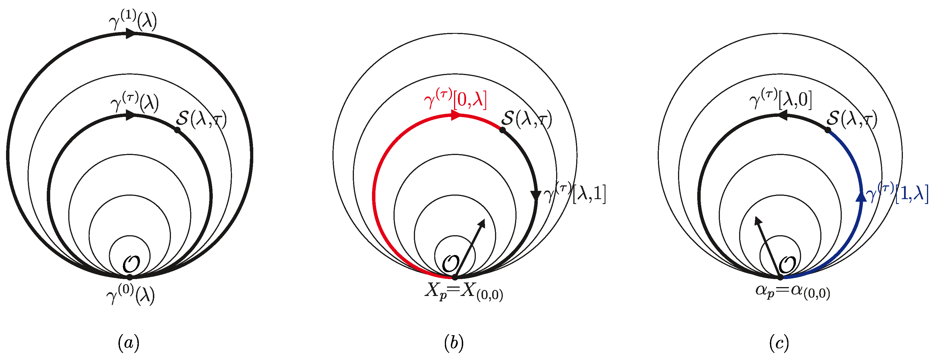
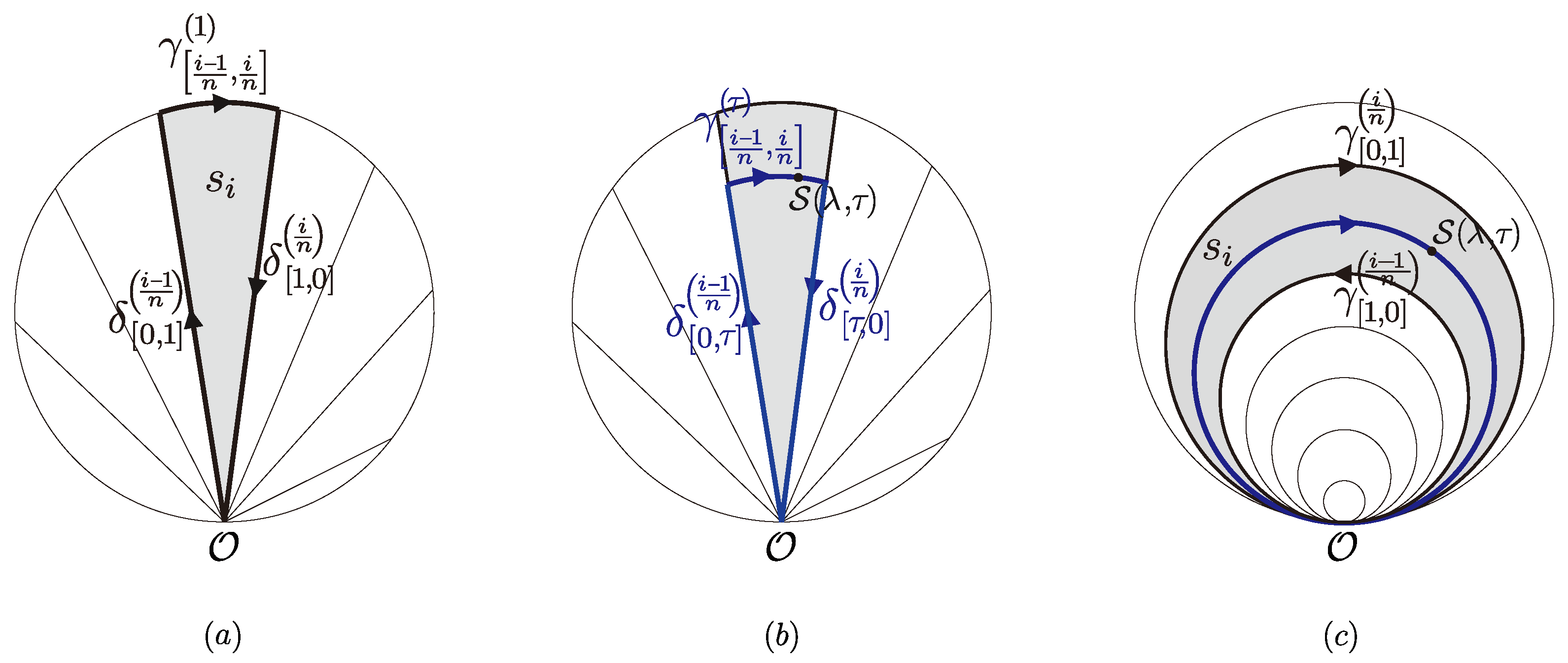
The covariant map, as an analog to (43), is defined as

$${\mathit{H}}_{{\delta }^{\left(\lambda \right)}\left[0,\tau \right]}^{*}\left({\beta }_{\left(0,0\right)}\right)={\beta }_{\left(0,0\right)}{\mathit{H}}_{{\delta }^{\left(\lambda \right)}\left[0,\tau \right]}^{*}={\beta }_{\left(\tau ,\lambda \right)},{\beta }_p\in T_p^{*}\mathcal{M}.$$

(59)

See Figure 2c for geometrical interpretation. Consequently:

(a)

Parallel transport of the covector field ${\beta }_{\left(\tau ,\lambda \right)}$ along ${\delta }^{\left(\lambda \right)}\left[0,\tau \right]$ satisfies

$${\nabla }_{{\partial }_{\tau }}{\beta }_{\left(\tau ,\lambda \right)}=0,\lambda \mathrm{fixed}.$$

(60)

(b)

For $\lambda =1,$${\beta }_{\left(0,0\right)}{\mathit{H}}_{{\delta }^{\left(1\right)}\left[0,\tau \right]}^{*}={\beta }_{\left(\tau ,1\right)},$ and moreover for $\tau =0,$${\beta }_{\left(0,0\right)}{\mathit{H}}_{{\delta }^{\left(1\right)}\left[0,0\right]}^{*}={\beta }_{\left(0,1\right)},$ which provides

$$\mathbb{I}{\beta }_{\left(0,0\right)}={\beta }_{\left(0,1\right)}.$$

(61)

(c)

For $\tau =0,$${\beta }_{\left(0,0\right)}{\mathit{H}}_{{\delta }^{\left(\lambda \right)}\left[0,0\right]}^{*}={\beta }_{\left(0,\lambda \right)}$, which provides $\mathbb{I}{\beta }_{\left(0,0\right)}={\beta }_{\left(0,\lambda \right)}$; therefore,

$${\nabla }_{{\partial }_{\lambda }}{\beta }_{\left(0,\lambda \right)}={\nabla }_{{\partial }_{\lambda }}{\beta }_{\left(0,0\right)}=0.$$

(62)

2.

The contravariant map, as an analog to (44), is defined as

$$\begin{array}{ccc}\hfill {\mathit{H}}_{{\gamma }^{\left(1\right)}\left[0,\lambda \right]}\left(Y_{\left(0,0\right)}\right)& =& Y_{\left(1,\lambda \right),}{Y}_p\in T_p\mathcal{M},\hfill \end{array}$$

(63)

$$\begin{array}{ccc}\hfill {\mathit{H}}_{{\delta }^{\left(\lambda \right)}\left[1,\tau \right]}\left(Y_{\left(1,\lambda \right)}\right)& =& Y_{\left(\tau ,\lambda \right).}\hfill \end{array}$$

(64)

See Figure 2b for the geometrical interpretation. Consequently:

(a)

Parallel transport of the vector field $Y_{\left(1,\lambda \right)}$ along ${\gamma }^{\left(1\right)}\left[0,\lambda \right]$ satisfies

$${\nabla }_{{\partial }_{\lambda }}{Y}_{\left(1,\lambda \right)}=0,\tau \mathrm{fixed}.$$

(65)

(b)

Parallel transport of the vector field $Y_{\left(\tau ,\lambda \right)}$ along ${\delta }^{\left(\lambda \right)}\left[1,\tau \right]$ satisfies

$${\nabla }_{{\partial }_{\tau }}{Y}_{\left(\tau ,\lambda \right)}=0,\lambda \mathrm{fixed}.$$

(66)

(c)

For $\tau =0,$${\mathit{H}}_{{\delta }^{\left(\lambda \right)}\left[1,0\right]}\left(Y_{\left(1,\lambda \right)}\right)=Y_{\left(0,\lambda \right),}$ which causes

$$\begin{array}{ccc}\hfill {\nabla }_{{\partial }_{\tau }}{Y}_{\left(0,\lambda \right)}& =& 0,\hfill \\ \hfill {\nabla }_{{\partial }_{\lambda }}{Y}_{\left(0,\lambda \right)}& \ne & 0,\mathrm{in}\mathrm{general}.\hfill \end{array}$$

(67)

(d)

Equations (63) and (64) together lead to $Y_{\left(\tau ,\lambda \right)}={\mathit{H}}_{{\delta }^{\left(\lambda \right)}\left[1,\tau \right]}{\mathit{H}}_{{\gamma }^{\left(1\right)}\left[0,\lambda \right]}{Y}_{\left(0,0\right)}$.

For $\tau =0,$$\lambda =1$, $Y_{\left(0,1\right)}=$${\mathit{H}}_{{\delta }^{\left(1\right)}\left[1,0\right]}$ ${\mathit{H}}_{{\gamma }^{\left(1\right)}\left[0,1\right]}$$\left(Y_{\left(0,0\right)}\right),$ and with ${\mathit{H}}_{{\delta }^{\left(1\right)}\left[1,0\right]}=\mathbb{I}$ (where $\lambda =1$ and $\lambda =0$ are identified, see Figure 2), we have

$$Y_{\left(0,1\right)}={\mathit{H}}_{{\gamma }^{\left(1\right)}\left[0,1\right]}\left(Y_{\left(0,0\right)}\right).$$

(68)

We can write a similar relation to (52), i.e., $⟨{\beta }_p,\Delta Y_p⟩=⟨{\beta }_{\left(0,0\right)},{\mathit{H}}_{{\gamma }^{\left(1\right)}\left[0,1\right]}\left(Y_{\left(0,0\right)}\right)-Y_{\left(0,0\right)}⟩$, then use (61) and (68) on the RHS to obtain

$$⟨{\beta }_p,\Delta Y_p⟩=⟨{\beta }_{\left(0,1\right)},Y_{\left(0,1\right)}⟩-⟨{\beta }_{\left(0,0\right)},Y_{\left(0,0\right)}⟩.$$

(69)

As previously (in (53)–(55)), we can obtain

$$⟨{\beta }_p,\Delta Y_p⟩=\underset{0}{\overset{1}{\int }}d\lambda ⟨{\beta }_{\left(0,\lambda \right)},{\nabla }_{{\partial }_{\lambda }}{Y}_{\left(0,\lambda \right)}⟩.$$

(70)

Following similar steps to the previous derivation in (55)–(57), with the help of relations (60)–(68) we can obtain the same result. Relation (58) remains valid; for any ${\beta }_p\in T_p^{*}\mathcal{M}$ and $Y_p\in T_p\mathcal{M}$,

$$⟨{\beta }_p,\left({\mathit{H}}_{{\gamma }^{\left(1\right)}\left[0,1\right]}-\mathbb{I}\right)Y_p⟩=⟨{\beta }_p,-\underset{\mathcal{S}}{\int }{\tilde{\mathit{R}}}_{\left(\mathcal{S}\left(\tau ,\lambda \right)\right)}\left(Y_p\right)⟩,$$

(71)

except with a different path-dependent twisted curvature, as follows:

$${\tilde{\mathit{R}}}_{\left(\mathcal{S}\left(\tau ,\lambda \right)\right)}={\mathit{H}}_{{\delta }^{\left(\lambda \right)}\left[\tau ,0\right]}{\mathit{R}}_{\left(\mathcal{S}\left(\tau ,\lambda \right)\right)}{\mathit{H}}_{{\delta }^{\left(\lambda \right)}\left[1,\tau \right]}{\mathit{H}}_{{\gamma }^{\left(1\right)}\left[0,\lambda \right]}.$$

(72)

The difference can be seen in the group elements of the ‘conjugation’ at the RHS of (72), which depends on the choice of curves. With these examples, it is apparent that relation (71) is invariant under at least two choices of parameterization, i.e., the choice of the family of loops. It is possible to propose the conjecture that relation in (58) and (71), and additionally the integral of the generalized twisted curvature in (23), are invariant under the choice of parameterization, i.e., the choice of the family of loops.

3.2.5. Gauge Transformation and Near-Zero Approximation

The relation in (58) and (71) is exact, as the steps in the derivation do not contain any approximations. However, the ‘conjugation’ in the generalized twisted curvature is not a gauge transformation. To obtain the gauge transformation, we can proceed with the following steps. First, Equation (70) can be written as

$$⟨{\beta }_p,\Delta Y_p⟩=\underset{0}{\overset{1}{\int }}d\lambda ⟨{\beta }_{\left(\tau ,\lambda \right)},{\nabla }_{{\partial }_{\lambda }}{Y}_{\left(\tau ,\lambda \right)}⟩$$

for $\tau =0$. Then, ${\nabla }_{{\partial }_{\lambda }}$ is the connection at ${\gamma }^{\left(\tau =0\right)}\left(\lambda \right)$ in the direction of ${\partial }_{\lambda }$. Writing ${\beta }_{\left(\tau ,\lambda \right)}$ and $Y_{\left(\tau ,\lambda \right)}$ as parallel-transported objects from $\mathcal{O}$, we obtain

$$\begin{array}{cc}\hfill ⟨{\beta }_p,\Delta Y_p⟩& =\underset{0}{\overset{1}{\int }}d\lambda ⟨{\beta }_{\left(0,0\right)}{\mathit{H}}_{{\delta }^{\left(\lambda \right)}\left[0,\tau \right]}^{*},{\nabla }_{{\partial }_{\lambda }}{\mathit{H}}_{{\delta }^{\left(\lambda \right)}\left[1,\tau \right]}{\mathit{H}}_{{\gamma }^{\left(1\right)}\left[0,\lambda \right]}{Y}_{\left(0,0\right)}⟩,\hfill \\ \hfill & =\underset{0}{\overset{1}{\int }}d\lambda ⟨{\beta }_{\left(0,0\right)},{\mathit{H}}_{{\delta }^{\left(\lambda \right)}\left[\tau ,0\right]}{\nabla }_{{\partial }_{\lambda }}{\mathit{H}}_{{\delta }^{\left(\lambda \right)}\left[1,\tau \right]}{\mathit{H}}_{{\gamma }^{\left(1\right)}\left[0,\lambda \right]}{Y}_{\left(0,0\right)}⟩,\tau =0,\hfill \end{array}$$

(73)

where in the last step we use parallel transport of the objects along the curve ${\delta }^{\left(\lambda \right)}\left[\tau ,0\right]$. The vector inside the inner product can be written as follows:

$${\mathit{H}}_{{\delta }^{\left(\lambda \right)}\left[\tau ,0\right]}{\nabla }_{{\partial }_{\lambda }}{\mathit{H}}_{{\delta }^{\left(\lambda \right)}\left[1,\tau \right]}{\mathit{H}}_{{\gamma }^{\left(1\right)}\left[0,\lambda \right]}{Y}_{\left(0,0\right)}={\mathit{H}}_{f\left(\tau ,\lambda \right)}{\partial }_{\lambda }{Y}_{\left(0,0\right)}+\tilde{\omega }{}_{{\gamma }^{\left(\tau \right)}\left(\lambda \right)}{Y}_{\left(0,0\right)},$$

(74)

where

$${\mathit{H}}_{f\left(\tau ,\lambda \right)}={\mathit{H}}_{{\delta }^{\left(\lambda \right)}\left[\tau ,0\right]}{\mathit{H}}_{{\delta }^{\left(\lambda \right)}\left[1,\tau \right]}{\mathit{H}}_{{\gamma }^{\left(1\right)}\left[0,\lambda \right]}$$

(75)

is the holonomy along loop $f\left(\lambda ,\tau \right)={\delta }^{\left(\lambda \right)}\left[\tau ,0\right]\circ {\delta }^{\left(\lambda \right)}\left[1,\tau \right]\circ {\gamma }^{\left(\tau \right)}\left[0,\lambda \right]$ (see Figure 2b) and

$$\tilde{\omega }{}_{{\gamma }^{\left(\tau \right)}\left(\lambda \right)}\left({\partial }_{\lambda }\right)={\mathit{H}}_{{\delta }^{\left(\lambda \right)}\left[\tau ,0\right]}\left({\partial }_{\lambda }+\omega {}_{{\gamma }^{\left(\tau \right)}\left(\lambda \right)}\left({\partial }_{\lambda }\right)\right){\mathit{H}}_{{\delta }^{\left(\lambda \right)}\left[1,\tau \right]}{\mathit{H}}_{{\gamma }^{\left(1\right)}\left[0,\lambda \right]}$$

(76)

is the generalized twisted connection at ${\gamma }^{\left(\tau \right)}\left[\lambda \right]$ in the direction of ${\partial }_{\lambda }$.

Let us now consider a special case of loops, where ${\delta }^{\left(\lambda \right)}\left[1,\tau \right]\circ {\gamma }^{\left(\tau \right)}\left[0,\lambda \right]={\delta }^{\left(\lambda \right)}\left[0,\tau \right]$ such that

$${\mathit{H}}_{{\delta }^{\left(\lambda \right)}\left[1,\tau \right]}{\mathit{H}}_{{\gamma }^{\left(1\right)}\left[0,\lambda \right]}={\mathit{H}}_{{\delta }^{\left(\lambda \right)}\left[\tau ,0\right].}^{-1}$$

(77)

With this, ${\mathit{H}}_{f\left(\tau ,\lambda \right)}=\mathbb{I}$, and the twisted connection $\tilde{\omega }{}_{{\gamma }^{\left(\tau \right)}\left(\lambda \right)}\left({\partial }_{\lambda }\right)$ becomes

$${\mathit{H}}_{{\delta }^{\left(\lambda \right)}\left[0,\tau \right]}^{-1}{\partial }_{\lambda }{\mathit{H}}_{{\delta }^{\left(\lambda \right)}\left[0,\tau \right]}+{\mathit{H}}_{{\delta }^{\left(\lambda \right)}\left[0,\tau \right]}^{-1}\omega {}_{{\gamma }^{\left(\tau \right)}\left(\lambda \right)}\left({\partial }_{\lambda }\right){\mathit{H}}_{{\delta }^{\left(\lambda \right)}\left[0,\tau \right]}=\omega {}_{{\gamma }^{\left(0\right)}\left(0\right)}\left({\partial }_{\lambda }\right):=-\omega \left({\partial }_{\lambda }\right).$$

(78)

Considering that the ${\mathit{H}}^{}$s are elements of $\mathcal{G},$ (78) is exactly the gauge transformation of $\omega {}_{{\gamma }^{\left(\tau \right)}\left(\lambda \right)}$ by ${\mathit{H}}_{{\delta }^{\left(\lambda \right)}\left[\tau ,0\right]}$ to $\omega ,$ i.e., the connection at the origin.

Let us now return to relation (74). At this point, we need to take an approximation. For small $\lambda$, the following approximation is valid:

$${\mathit{H}}_{{\delta }^{\left(\lambda \right)}\left[\tau ,1\right]}{\mathit{H}}_{{\delta }^{\left(\lambda \right)}\left[0,\tau \right]}\approx {\mathit{H}}_{{\gamma }^{\left(1\right)}\left[0,\lambda \right]};$$

(79)

see Figure 2. Note that this approximate relation is exactly the condition (77) which gives rise to the gauge transformation (78) from the twisted connection (76). Hence, in this limit, (73) becomes

$$\begin{array}{cc}\hfill ⟨{\beta }_p,\Delta Y_p⟩& =\underset{0}{\overset{1}{\int }}d\lambda ⟨{\beta }_{\left(0,0\right)},{\mathit{H}}_{f\left(\tau ,\lambda \right)}{\partial }_{\lambda }{Y}_{\left(0,0\right)}+\tilde{\omega }{}_{{\gamma }^{\left(\tau \right)}\left(\lambda \right)}\left({\partial }_{\lambda }\right)Y_{\left(0,0\right)}⟩,\hfill \\ \hfill & \approx ⟨{\beta }_{\left(0,0\right)},Y_{\left(0,0\right)}⟩+⟨{\beta }_{\left(0,0\right)},-\underset{0}{\overset{1}{\int }}d\lambda \omega Y_{\left(0,0\right)}⟩,\hfill \end{array}$$

with (78) and ${\mathit{H}}_{f\left(\tau ,\lambda \right)}=\mathbb{I}$. Because the pair $\left({\beta }_p,Y_p\right)$ could be any vector and covector, we choose them here such that $⟨{\beta }_p,Y_p⟩=⟨{\beta }_{\left(0,0\right)},Y_{\left(0,0\right)}⟩=0,$ and obtain

$$⟨{\beta }_p,\left({\mathit{H}}_{{\gamma }^{\left(1\right)}\left[0,1\right]}-\mathbb{I}\right)Y_p⟩\approx ⟨{\beta }_{\left(0,0\right)},-\underset{0}{\overset{1}{\int }}d\lambda {\omega }_{\mathcal{O}}\left({\partial }_{\lambda }\right)\left(Y_{\left(0,0\right)}\right)⟩=⟨{\beta }_p,-{\oint }_{\gamma }\omega \left(Y_p\right)⟩.$$

(80)

It is important to keep in mind that the relation is valid for small $\lambda$, which means that this is an approximation of ${\gamma }^{\left(1\right)}\left[0,1\right]$ near the origin $\mathcal{O}$.

Now, we can apply the same near-zero limit to (71) by applying condition (79) to the generalized twisted curvature (72), which becomes the original twisted curvature

$${\overline{\mathit{R}}}_{\left(\mathcal{S}\left(\tau ,\lambda \right)\right)}={\mathit{H}}_{{\delta }^{\left(\lambda \right)}\left[0,\tau \right]}^{-1}{\mathit{R}}_{\left(\mathcal{S}\left(\tau ,\lambda \right)\right)}{\mathit{H}}_{{\delta }^{\left(\lambda \right)}\left[0,\tau \right]}$$

(81)

with the standard action of group conjugation. With this, (71) can be written as

$$⟨{\beta }_p,\left({\mathit{H}}_{{\gamma }^{\left(1\right)}\left[0,1\right]}-\mathbb{I}\right)Y_p⟩\approx ⟨{\beta }_p,-\underset{\mathcal{S}}{\int }{\overline{\mathit{R}}}_{\left(\mathcal{S}\left(\tau ,\lambda \right)\right)}\left(Y_p\right)⟩.$$

(82)

Following the derivation, from Equations (80) and (82) we can obtain the near-zero approximation of the holonomy along a loop in terms of the connection and the curvature form. We state the result as the following theorem.

Theorem 1.

The near-zero approximation of a holonomy along a closed loop ${\gamma }^{\left(1\right)}\left[0,1\right]$ as the boundary of a surface $\mathcal{S}\left(\lambda ,\tau \right)$ satisfying (17)–(20) is

$$\left(\underset{\tau ,\lambda \to 0}{lim}{\mathit{H}}_{{\gamma }^{\left(1\right)}\left[0,1\right]}\right)Y_p\approx \left(\mathbb{I}-{\oint }_{\gamma }\omega \right)Y_p,\forall Y_p\in T_p\mathcal{M},$$

(83)

where ω is the connection coefficient of the connection ∇, or

$$\left(\underset{\lambda \to 0}{lim}{\mathit{H}}_{{\gamma }^{\left(1\right)}\left[0,1\right]}\right)Y_p\approx \left(\mathbb{I}-\underset{\mathcal{S}}{\int }{\overline{\mathit{R}}}_{\left(\mathcal{S}\left(\tau ,\lambda \right)\right)}\right)Y_p,$$

(84)

with ${\overline{\mathit{R}}}_{\left(\mathcal{S}\left(\tau ,\lambda \right)\right)}$ being the twisted curvature of the connection, which satisfies (81).

Moreover, because they are obtained at a same limit, we can compare Equations (83) and (84) to obtain the relation.

Corollary 1.

For a given a closed loop ${\gamma }^{\left(1\right)}\left[0,1\right]$ as the boundary of surface $\mathcal{S}\left(\lambda ,\tau \right)$ satisfying (17)–(20), the following equality, usually known as the non-Abelian Stokes theorem in two dimensions, is valid:

$${\oint }_{\gamma }\omega =\underset{\mathcal{S}}{\int }{\overline{\mathit{R}}}_{\left(\mathcal{S}\left(\tau ,\lambda \right)\right),}$$

(85)

where ω is the connection 1-form and ${\overline{\mathit{R}}}_{\left(\mathcal{S}\left(\tau ,\lambda \right)\right)}$ is the twisted curvature 2-form of the connection, satisfying (81).

With this, our derivation in this article can be viewed as an alternative proof for the non-Abelian Stokes theorem in two dimensions. From the derivation, it can be argued that relation (85) is only valid in the regime of near-zero limit; in the next section, we show that this is not the case.

3.3. The Exact Relation

In this section, we derive the exact relation between the holonomy along the loop with the curvature 2-form through a non-algebraic approach. The result is similar to those in [5,6,7,8].

3.3.1. Finite Partition of a Surface

Let us first define a finite partition on the homotopic surface $\mathcal{S}\left(\lambda ,\tau \right)$, as described in Figure 3a.

Figure 3. (a) A partition $s_i$ of $\mathcal{S}\left(\tau ,\lambda \right)$ (the grey area) with its boundary ${\gamma }_i$ (in black). Notice that if the number of partitions n grows larger, $s_i$ becomes narrower such that ${\delta }^{\left(\frac{i-1}{n}\right)}$ and ${\delta }^{\left(\frac{i}{n}\right)}$ coincide. (b) The curvature form at point $\mathcal{S}\left(\lambda ,\tau \right)$, where ${\mathit{R}}_{\mathcal{S}\left(\lambda ,\tau \right)}$ is parallel-transported to $\mathcal{O}$ by loop ${\psi }_i^{\left(\tau \right)}={\delta }_{\left[\tau ,0\right]}^{\left(\frac{i}{n}\right)}\circ {\gamma }_{\left[\frac{i-1}{n},\frac{i}{n}\right]}^{\left(\tau \right)}\circ {\delta }_{\left[0,\tau \right]}^{\left(\frac{i-1}{n}\right)}$ (in blue). (c). A different partition $s_i$ of $\mathcal{S}\left(\tau ,\lambda \right)$ (the grey area), with its boundary ${\gamma }_i={\gamma }_{\left[1,0\right]}^{\left(\frac{i-1}{n}\right)}\circ {\gamma }_{\left[0,1\right]}^{\left(\frac{i}{n}\right)}$ (in black). ${\mathit{R}}_{\mathcal{S}\left(\lambda ,\tau \right)}$ is parallel-transported to $\mathcal{O}$ by loop ${\gamma }_{\left[0,1\right]}^{\left(\tau \right)}$ (in blue) with $\frac{i-1}{n}\le \tau \le \frac{i}{n}$.

Let each element of the partition be labeled by $s_i$ such that ${\bigcup }_{i=1}^n{s}_i=\mathcal{S}$. The partition on $\mathcal{S}$ induces a partition on the boundary $\gamma$ such that ${\bigcup }_{i=1}^n{\gamma }_i=\gamma .$ To be more precise, we can define ${\gamma }_i$ as follows:

$${\gamma }_i={\gamma }_{\left[{\lambda }_{\mathrm{init}}=\frac{i-1}{n},{\lambda }_{\mathrm{fin}}=\frac{i}{n}\right]}^{\left(\tau =1\right)},={\gamma }_{\left[\frac{i-1}{n},\frac{i}{n}\right]}^{\left(1\right)},$$

then, the boundary $\gamma$ can be written as

$$\gamma ={\gamma }_{\left[0,1\right]}^{\left(1\right)}={\gamma }_{\left[\frac{n-1}{n},1\right]}^{\left(1\right)}\circ \cdots \circ {\gamma }_{\left[\frac{i-1}{n},\frac{i}{n}\right]}^{\left(1\right)}\circ \cdots \circ {\gamma }_{\left[\frac{1}{n},\frac{2}{n}\right]}^{\left(1\right)}\circ {\gamma }_{\left[0,\frac{1}{n}\right]}^{\left(1\right)}.$$

Moreover, each partition $s_i\left(\lambda ,\tau \right)$ has a boundary ${\psi }_i$ satisfying

$${\psi }_i={\delta }_{\left[1,0\right]}^{\left(\frac{i}{n}\right)}\circ {\gamma }_{\left[\frac{i-1}{n},\frac{i}{n}\right]}^{\left(1\right)}\circ {\delta }_{\left[0,1\right]}^{\left(\frac{i-1}{n}\right)},{\delta }_{\left[a,b\right]}^{\left(c\right)}={\delta }_{\left[{\tau }_{\mathrm{init}}=a,{\tau }_{\mathrm{fin}}=b\right]}^{\left(\lambda =c\right)}.$$

It can easily be shown that the product of all ${\psi }_i$s provides us with ${\gamma }_{\left[0,1\right]}^{\left(1\right)}$, as the internal terms (the $\delta$s) cancel each other:

$$\prod _{i=1}^n{\psi }_i=\underset{\mathbb{I}}{\underbrace{{\delta }_{\left[1,0\right]}^{\left(1\right)}}}\circ {\gamma }_{\left[\frac{n-1}{n},1\right]}^{\left(1\right)}\circ {\delta }_{\left[0,1\right]}^{\left(\frac{n-1}{n}\right)}\circ \cdots {\delta }_{\left[1,0\right]}^{\left(\frac{2}{n}\right)}\circ {\gamma }_{\left[\frac{1}{n},\frac{2}{n}\right]}^{\left(1\right)}\circ \underset{\mathbb{I}}{\underbrace{{\delta }_{\left[0,1\right]}^{\left(\frac{1}{n}\right)}\circ {\delta }_{\left[1,0\right]}^{\left(\frac{1}{n}\right)}}}\circ {\gamma }_{\left[0,\frac{1}{n}\right]}^{\left(1\right)}\circ \underset{\mathbb{I}}{\underbrace{{\delta }_{\left[0,1\right]}^{\left(0\right)}}}={\gamma }_{\left[0,1\right]}^{\left(1\right)}.$$

3.3.2. Ordered Product of Holonomies

Similar rules are followed by the holonomies along these curves, with $X_p\in T_p\mathcal{M}$:

$$\begin{array}{cc}\hfill {\mathit{H}}_{\gamma }\left(X_p\right)& =\left({\mathit{H}}_{{\gamma }_n}\cdots {\mathit{H}}_{{\gamma }_i}\cdots {\mathit{H}}_{{\gamma }_2}{\mathit{H}}_{{\gamma }_1}\right)\left(X_p\right),\hfill \end{array}$$

(86)

$$\begin{array}{cc}\hfill {\mathit{H}}_{{\psi }_i}\left(X_p\right)& =\left({\mathit{H}}_{{\delta }_{\left[1,0\right]}^{\left(\frac{i}{n}\right)}}{\mathit{H}}_{{\gamma }_i}{\mathit{H}}_{{\delta }_{\left[0,1\right]}^{\left(\frac{i-1}{n}\right)}}\right)\left(X_p\right),\hfill \end{array}$$

(87)

$$\begin{array}{cc}\hfill {\mathit{H}}_{\gamma }\left(X_p\right)& =\left({\mathit{H}}_{{\psi }_n}\cdots {\mathit{H}}_{{\psi }_i}\cdots {\mathit{H}}_{{\psi }_2}{\mathit{H}}_{{\psi }_1}\right)\left(X_p\right).\hfill \end{array}$$

(88)

The nearly flat limit approximation (84) becomes valid a sufficiently large number of partitions n, as the curve ${\delta }_{\left[0,1\right]}^{\left(\frac{i-1}{n}\right)}$ becomes closer to ${\delta }_{\left[0,1\right]}^{\left(\frac{i}{n}\right)}$ as n grows larger, while $s_i$ becomes narrower; see Figure 3a. Using the fact that (84) is valid for arbitrary loops as well as arbitrary parameterizations, the holonomy along the boundary of partition $s_i\left(\lambda ,\tau \right)$ can be approximated using Theorem 1:

$${\mathit{H}}_{{\psi }_i}\approx \mathbb{I}-\underset{s_i}{\int }{\tilde{\mathit{R}}}_{\left(i\right)},$$

(89)

where the generalized twisted curvature ${\tilde{\mathit{R}}}_{\left(i\right)}$ of $s_i$ satisfies

$${\tilde{\mathit{R}}}_{\left(i\right)}={\mathit{H}}_{{\delta }_{\left[\tau ,0\right]}^{\left(\frac{i}{n}\right)}}{\mathit{H}}_{{\gamma }_{\left[\lambda ,\frac{i}{n}\right]}^{\left(\tau \right)}}{\left.\mathit{R}\right|}_{\mathcal{S}\left(\tau ,\lambda \right)}{\mathit{H}}_{{\gamma }_{\left[\frac{i-1}{n},\lambda \right]}^{\left(\tau \right)}}{\mathit{H}}_{{\delta }_{\left[0,\tau \right]}^{\left(\frac{i-1}{n}\right)}},0\le \tau \le 1,\frac{i-1}{n}\le \lambda \le \frac{i}{n};$$

(90)

see Figure 3b. The holonomy around $\gamma$ can be obtained from relation (88):

$${\mathit{H}}_{{\gamma }_{\left[0,1\right]}^{\left(1\right)}}=\prod _{i=1,\leftarrow }^n{\mathit{H}}_{{\psi }_i}\approx \prod _{i=1,\leftarrow }^n\left(\mathbb{I}-\underset{s_i}{\int }{\tilde{\mathit{R}}}_{\left(i\right)}\right),$$

(91)

with the ← sign on the product a reminder that the holonomies subjected to ∏ are ordered as the left action, i.e., ${\mathit{H}}_{{\psi }_i}\cdots {\mathit{H}}_{{\psi }_2}{\mathit{H}}_{{\psi }_1}$. Equation (91) is valid for sufficiently large n.

3.3.3. The Continuous Limit and Volterra Product Integral

Now, let us take the number of partitions $n\to \infty$; the partition s becomes infinitesimal ($ds$) and the validity of (89) reaches exactness. The discrete product ∏ becomes a product integral, labeled by ${\prod }_a^b$, which is a product analog for the integral ∫ as a continuous limit of the Riemann sum ∑, while $\left[a,b\right]$ is the interval of the product integral. Equation (91) then becomes

$${\mathit{H}}_{{\gamma }_{\left[0,1\right]}^{\left(1\right)}}=\underset{n\to \infty }{lim}{\displaystyle \prod _{i=1,\leftarrow }^n}{\mathit{H}}_{{\psi }_i}=\underset{{\prod }_{\lambda =0}^{\lambda =1}}{\underbrace{\underset{n\to \infty }{lim}\prod _{i=1,\leftarrow }^n}}\underset{n\to \infty }{lim}{\mathit{H}}_{{\psi }_i}.$$

With (89), the quantity ${\displaystyle \underset{n\to \infty }{lim}}{\mathit{H}}_{{\psi }_i}$ can be written as follows:

$$\underset{n\to \infty }{lim}{\mathit{H}}_{{\psi }_i}=\mathbb{I}-\underset{n\to \infty }{lim}\underset{s_i}{\int }{\tilde{\mathit{R}}}_{\left(i\right)},$$

where

$$\begin{array}{cc}\hfill {\underset{n\to \infty }{lim}}_{\underset{s_i}{\int }}{\tilde{\mathit{R}}}_{\left(i\right)}& =\underset{n\to \infty }{lim}\underset{\lambda =\frac{i-1}{n}}{\overset{\lambda =\frac{i}{n}}{\int }}\underset{\tau =0}{\overset{\tau =1}{\int }}{\mathit{H}}_{{\delta }_{\left[\tau ,0\right]}^{\left(\frac{i}{n}\right)}}{\mathit{H}}_{{\gamma }_{\left[\lambda ,\frac{i}{n}\right]}^{\left(\tau \right)}}{\left.{\mathit{R}}_{\tau \lambda }\right|}_{\mathcal{S}\left(\tau ,\lambda \right)}{\mathit{H}}_{{\gamma }_{\left[\frac{i-1}{n},\lambda \right]}^{\left(\tau \right)}}{\mathit{H}}_{{\delta }_{\left[0,\tau \right]}^{\left(\frac{i-1}{n}\right)}}d\tau d\lambda ,\hfill \\ \hfill & =\underset{\tau =0}{\overset{\tau =1}{\int }}{\mathit{H}}_{{\delta }_{\left[\tau ,0\right]}^{\left(\lambda \right)}}{\left.{\mathit{R}}_{\tau \lambda }\right|}_{\mathcal{S}\left(\tau ,\lambda \right)}{\mathit{H}}_{{\delta }_{\left[0,\tau \right]}^{\left(\lambda \right)}}d\tau d\lambda \hfill \end{array}$$

per the Fundamental Theorem of Calculus. Therefore, we have

$${\mathit{H}}_{{\gamma }_{\left[0,1\right]}^{\left(1\right)}}=\prod _{\lambda =0,\leftarrow }^{\lambda =1}\left(\mathbb{I}-\underset{\tau =0}{\overset{\tau =1}{\int }}{\mathit{H}}_{{\delta }_{\left[\tau ,0\right]}^{\left(\lambda \right)}}{\left.{\mathit{R}}_{\tau \lambda }\right|}_{\mathcal{S}\left(\tau ,\lambda \right)}{\mathit{H}}_{{\delta }_{\left[0,\tau \right]}^{\left(\lambda \right)}}d\tau d\lambda \right).$$

(92)

At this point, it is necessary to introduce the Volterra product integral [10]. Let $A\left(x\right)$ be a (Riemann-integrable) matrix-valued function; then, the following left (and right) product integral exists:

$$\begin{array}{cc}\hfill \prod _{a,\leftarrow }^b\left(\mathbb{I}+A\left(x\right)dx\right)=& \mathbb{I}+\underset{a}{\overset{b}{\int }}A\left(x\right)dx+\underset{a}{\overset{b}{\int }}\underset{x_1=a}{\overset{x_1=x_2}{\int }}A\left(x_2\right)A\left(x_1\right)d{x}_{1}d{x}_2\hfill \\ \hfill & +\underset{a}{\overset{b}{\int }}\underset{x_2=a}{\overset{x_2=x_3}{\int }}\underset{x_1=a}{\overset{x_1=x_2}{\int }}A\left(x_3\right)A\left(x_2\right)A\left(x_1\right)d{x}_{1}d{x}_{2}d{x}_3+\cdots ,\hfill \end{array}$$

(93)

for $b\ge \cdots \ge x_2\ge x_1\ge a$. For simplicity, we only provide the definition of the left product integral. Moreover, (93) can be written as

$$\begin{array}{cc}\hfill \prod _{a,\leftarrow }^b\left(\mathbb{I}+A\left(x\right)dx\right)& ={\widehat{P}}_{x}exp\underset{a}{\overset{b}{\int }}A\left(x\right)dx,\hfill \end{array}$$

(94)

where ${\widehat{P}}_x$ is the path-ordered operator. Using (94) on (92), we obtain the following equation:

$${\mathit{H}}_{{\gamma }_{\left[0,1\right]}^{\left(1\right)}}={\widehat{P}}_{\lambda }exp-\underset{0}{\overset{1}{\int }}\underset{0}{\overset{1}{\int }}{\mathit{H}}_{{\delta }_{\left[0,\tau \right]}^{\left(\lambda \right)}}^{-1}{\left.{\mathit{R}}_{\tau \lambda }\right|}_{\mathcal{S}\left(\tau ,\lambda \right)}{\mathit{H}}_{{\delta }_{\left[0,\tau \right]}^{\left(\lambda \right)}}d\tau d\lambda ={\widehat{P}}_{\gamma }exp-\underset{\mathcal{S}}{\int }\overline{\mathit{R}},$$

(95)

where the path-ordered operator ${\widehat{P}}_{\gamma }$ acts along $\gamma \left(\lambda \right)$ and $\overline{\mathit{R}}$ is the standard twisted curvature in (81).

It is possible to use a different partition of $\mathcal{S}$ to obtain a similar result. For example, let us consider a different partition from the one in Figure 3c, with the generalized twisted curvature ${\tilde{\mathit{R}}}_{\left(i\right)}$ of $s_i$ satisfying

$${\tilde{\mathit{R}}}_{\left(i\right)}={\mathit{H}}_{{\gamma }_{\left[\lambda ,0\right]}^{\left(\frac{i}{n}\right)}}{\mathit{H}}_{{\delta }_{\left[\tau ,\frac{i}{n}\right]}^{\left(\lambda \right)}}{\left.\mathit{R}\right|}_{\mathcal{S}\left(\tau ,\lambda \right)}{\mathit{H}}_{{\delta }_{\left[\frac{i-1}{n},\tau \right]}^{\left(\lambda \right)}}{\mathit{H}}_{{\gamma }_{\left[0,\lambda \right]}^{\left(\frac{i-1}{n}\right)}},0\le \lambda \le 1,\frac{i-1}{n}\le \tau \le \frac{i}{n}.$$

(96)

A similar derivation yields

$${\mathit{H}}_{{\gamma }^{\left(1\right)}\left[0,1\right]}{X}_p=\left({\widehat{P}}_{\delta \left(\tau \right)}exp-\underset{\mathcal{S}}{\int }\overline{\mathit{R}}\right)X_p,X_p\in T_p\mathcal{M},$$

(97)

while with the standard twisted curvature $\overline{\mathit{R}}$ satisfying

$${\overline{\mathit{R}}}_{\left(\mathcal{S}\left(\tau ,\lambda \right)\right)}={\mathit{H}}_{{\gamma }^{\left(\tau \right)}\left[0,\lambda \right]}^{-1}{\mathit{R}}_{\left(\mathcal{S}\left(\tau ,\lambda \right)\right)}{\mathit{H}}_{{\gamma }^{\left(\tau \right)}\left[0,\lambda \right]}$$

(98)

instead of (81). Notice that the differences between (95) and (97) are on the path-ordering operator $\widehat{P}$ and on the group elements of the conjugation of $\overline{\mathit{R}}$. Different choices for partitioning $\mathcal{S}$ will affect these two objects but not the holonomy along the boundary, at least for the two parametrizations used in this work.

Finally, we can formulate the following theorem.

Theorem 2.

The holonomy along a closed loop ${\gamma }^{\left(1\right)}\left[0,1\right]$ as the boundary of a surface $\mathcal{S}\left(\lambda ,\tau \right)$ satisfying (17)–(20) is

$${\mathit{H}}_{{\gamma }^{\left(1\right)}\left[0,1\right]}{X}_p=\left({\widehat{P}}_{\delta }exp-\underset{\mathcal{S}}{\int }\overline{\mathit{R}}\right)X_p,X_p\in T_p\mathcal{M},$$

(99)

where ${\overline{\mathit{R}}}_{\left(\mathcal{S}\left(\lambda ,\tau \right)\right)}$ satisfies (98) (or (81), with ${\widehat{P}}_{\delta }$ replaced by ${\widehat{P}}_{\gamma }$).

With relation (99), we can finally obtain an exact relation between the holonomy and the curvature 2-form. The LHS and RHS of (99) are both in $\mathcal{G}$, as the exponential of integral $\overline{\mathit{R}}$, which is an element of the algebra $\mathfrak{g}$, is in $\mathcal{G}$. Hence, it is exact and valid for arbitrary affine connections.

Relation (99) is a well-known result, and has been studied, for example, in [5,6,7,8]. Our work in this article can be viewed as an alternative way to derive this relation. However, our derivation contains the following generalizations. (a) The derivation is valid for an arbitrary (boundary) loop; in [6], the derivation is carried out for a parallelogram with a specific square partition. (b) The ordered operator $\widehat{P}$ in the RHS of (99) is a path-ordering operator ${\widehat{P}}_{\delta }$ dictated by the loop $\delta$ (or ${\widehat{P}}_{\gamma }$ dictated by $\gamma$ if the twisted curvature is (81)); on the other hand, [6,7] used the surface-ordering operator ${\widehat{P}}_{\mathcal{S}}$. (c) We have found that different choices of partition for $\mathcal{S}$ affects the path-dependent twisted curvature via the group element in the conjugation, as well as the path-ordering operator; the path-ordering operator acts in the direction independent to the families of loops chosen as partitions of $\mathcal{S}$. (d) However, the relation (99) is invariant under different choices of partition and family of loops as a parameterization of $\mathcal{S}$, at least for the two cases of parameterization considered in this article.

3.3.4. Comments on Non-Abelian Stokes Theorem

Comparing relation (16) and (95), it is possible to exactly obtain the non-Abelian Stokes theorem for two dimensions. Therefore, relation (85) is not resticted to the near-zero limit, and is valid anywhere. Writing the theorem in the form of (85) is possible, as both the RHS of (16) and (95) use the same path-ordering operator ${\widehat{P}}_{\gamma }$. In [6,7], because one of the equations uses the surface-ordering operator ${\widehat{P}}_{\mathcal{S}}$, the theorem is written as ${\widehat{P}}_{\gamma }exp\underset{\gamma }{\oint }\omega ={\widehat{P}}_{\mathcal{S}}exp\underset{\mathcal{S}}{\int }\overline{\mathit{R}}$. Through a specific choice of partition on $\mathcal{S}$ (as in Figure 3a), it is possible to fix the 2D path-ordered operator to coincide with the 1D one, thereby obtaining (85).

A closer look at relation (99) indicates that the LHS, i.e., the holonomy ${\mathit{H}}_{{\gamma }^{\left(1\right)}\left[0,1\right]}$, depends only on the loop ${\gamma }^{\left(1\right)}\left[0,1\right]$, while the RHS, i.e., the twisted curvature ${\overline{\mathit{R}}}_{\left(\mathcal{S}\left(\lambda ,\tau \right)\right)}$, depends on the surface enclosed by the loop, that is, $\mathcal{S}\left(\lambda ,\tau \right)$. As already mentioned at the beginning of this section, there may be many surfaces sharing an identical boundary; hence, the relations (84) and (99) remain valid with a change of the evaluation surface $\mathcal{S}\left(\lambda ,\tau \right)\mapsto {\mathcal{S}}^{\prime }\left(\lambda ,\tau \right)$ as long as they share the same boundary $\partial {\mathcal{S}}^{\prime }\left(\lambda ,\tau \right)=\partial \mathcal{S}\left(\lambda ,\tau \right)={\gamma }^{\left(1\right)}\left[0,1\right]$. Hence, (99) clearly describes the bulk–boundary relation of the Stokes theorem.

The non-Abelian Stokes theorem for 2D has been studied extensively, for example, in [6], where it was derived through the operator and path-integral approach, in [7,8], where it was derived through the product integral approach, and in [11,12], where it was proven from a category theory perspective and remains an interesting subject to pursue.

4. Discussions and Conclusions

4.1. Discussion

We first review the ambiguity concerning the small loop approximation of the holonomy, as follows: consider an oriented manifold $\left(\mathcal{M},g,\nabla \right)$ where the curvature form ${\mathit{R}}_{\mathcal{S}\left(\lambda ,\tau \right)}$ of an affine connection ∇ is defined on each point of the manifold. For a given loop $\gamma$ embedded in $\mathcal{M}$ with origin point $\mathcal{O}$, it is possible to obtain the corresponding holonomy $\mathit{H}\left(\gamma ,\mathcal{O}\right)$ along the loop. For a manifold with dimension larger than 2, it is possible to construct infinitely many continuous (not necessarily smooth) surfaces $\mathcal{S}$ that can possibly be enclosed by the loop $\gamma =\partial \mathcal{S}$ as the boundary of $\mathcal{S}$. The non-uniqueness of $\mathcal{S}$ does not become a problem for the holonomy, as it does not depend on the surface, only on the loop. However, a problem appears if we consider the infinitesimal limit of the loop, that is, when the loop is shrunk to a point. As the loop shrinks, the holonomy (which is an element of a Lie group) changes accordingly. At the shrinking point, it is approximated by the Lie algebra element coming from the curvature form $\mathit{R}\left(\sigma \right)$. To obtain a specific Lie algebra from the local curvature form, $\mathit{R}\left(..,..\right)$ needs to act on a specific plane $\sigma$. The information of only the loop $\gamma$ and the holonomy $\mathit{H}\left(\gamma ,\mathcal{O}\right)$, is insufficient to determine the plane $\sigma$. In the following paragraph, we show that specifying the evaluation surface $\mathcal{S}$ is a solution to the ambiguity.

We have three relations with different ranges of validity. The first is relation (99) from Theorem 2 on the exact relation between a holonomy around a loop and the curvature form over the surface as defined in the non-local and finite setting:

$${\mathit{H}}_{\partial \mathcal{S}\left(\lambda ,\tau \right)}={\widehat{P}}_{\gamma }exp-\underset{\mathcal{S}\left(\lambda ,\tau \right)}{\int }\overline{\mathit{R}}.$$

The second is relation (84) from Theorem 1 on the near zero approximation of a holonomy along a loop as defined in the non-local and infinitesimal setting:

$$\underset{\lambda \to 0}{lim}{\mathit{H}}_{\partial \mathcal{S}\left(\lambda ,\tau \right)}=\mathbb{I}-\underset{\mathcal{S}\left(\lambda ,\tau \right)}{\int }\overline{\mathit{R}}.$$

The last is relation (7) on the small loop approximation of a holonomy around a loop as defined in the local and infinitesimal setting:

$$\underset{\lambda ,\tau \to 0}{lim}{\mathit{H}}_{\partial \mathcal{S}\left(\lambda ,\tau \right)}={\mathit{h}}_{\partial \mathcal{S}\left(\lambda ,\tau \right)}=\mathbb{I}-{\left.\mathit{R}\left(\sigma \right)\right|}_{\mathcal{O}},$$

where we are only concerned with the first leading-order term. Here, ${\mathit{h}}_{\partial \mathcal{S}\left(\lambda ,\tau \right)}$ is the local holonomy and the (evaluation) plane $\sigma$ is simply the surface $\mathcal{S}$ when $\tau \to 0$, namely, $\sigma =\underset{\tau \to 0}{lim}\mathcal{S}.$ All these equations fit nicely; the nearly flat approximation can be obtained by keeping the first leading order of the Dyson series on the exact relation, while the small loop approximation can be obtained from the nearly flat approximation simply by taking $\tau \to 0$; this is due to the fact that the curvature will necessarily be small when taking the small loop limit, while the converse is not the case. The clear relation between the non-local finite and the local infinitesimal objects in these equations can be obtained using the specification of the evaluation surface $\mathcal{S}$. With this, the ambiguity in obtaining a specific $\sigma$ given only the boundary loop $\gamma$ vanishes by ‘fixing’ the bulk $\mathcal{S}$, as we have mentioned previously.

The origin of the ambiguity can be traced to its root, namely, the redundancy of the choice of $\mathcal{S}$. We are already familiar with the fact that many surfaces can share a common boundary $\partial \mathcal{S}$; as seen in Theorems 1 and 2, the choice of $\mathcal{S}$ does not affect the holonomy ${\mathit{H}}_{\partial \mathcal{S}\left(\lambda ,\tau \right)}$, as it only depends on $\partial S$ and can be calculated independently from the exponential of (the integral of) the connection in (13) without mentioning $\mathcal{S}$ at all. The problem becomes apparent only when we consider the small loop limit, as the existence of $\sigma$ in the RHS requires $\mathcal{S}$ to be specified. In other words, a change of $\mathcal{S}\to {\mathcal{S}}^{\prime }$ validates Theorems 1 and 2 as long as the boundary $\partial \mathcal{S}$ does not change. We have already mentioned in Section 3 that Theorem 1 gives rise to the (non-Abelian) Stokes theorem for a surface. In fact, our work in this article provides an alternative proof for the theorem:

$$\underset{\gamma }{\oint }\omega =\underset{\mathcal{S}}{\int }\tilde{\mathit{R}},$$

which follows directly from comparing the standard definition of holonomy on a loop (in terms of connection) with relation (95) in Theorem 2. The formulation of the holonomy entirely as an exponential of an integral of the connection along the boundary, as in (13), is possible because the curvature 2-form is ‘exact’, that is, it is a differential (more precisely, the exterior covariant derivative) of the connection: $\mathit{R}={\mathrm{d}}_{\nabla }\omega$. Moreover, $\mathit{R}$ is ‘closed’, that is, ${\mathrm{d}}_{\nabla }\mathit{R}=0$, which is known as the (second) Bianchi identity. A generalization of the ‘line’ 1-holonomy, i.e., the ‘surface’ 2-holonomy, is possible for cases where the 2-form is not exact (and consequently not closed). This has been studied under the subject of 2-groups, 2-Lie algebras, and 2-connections; for examples, see [11,12,13,14].

All of our results are valid for any arbitrary loop and general affine connection on the tangent bundle $T\mathcal{M}={\bigcup }_p\left\{p\right\}\times T_p\mathcal{M}$. Furthermore, generalization to vector (and principal) bundles is straightforward.

4.2. Conclusions

Our work in this article can be summarized as follows. At the beginning of Section 2.1, we have provided a review of the curvature 2-form of an affine connection. As a complement to the terminologies in [9], namely, the loop orientation and the rotation bivector, we propose a new terminology, the evaluation plane $\sigma$, which the loop orientation acts upon to provide a Lie algebra element $\mathit{R}\left(\sigma \right)$.

In Section 2.2, we have presented a review of parallel transport and holonomy. Another new term we propose on this subject is the evaluation surface $\mathcal{S}$, defined as the surface enclosed by a loop where the holonomy is evaluated.

In Section 3.1, we identify an ambiguity concerning the small loop approximation of the holonomy, which is the main problem addressed in this article. The information of only the loop $\gamma$ and the non-local finite holonomy $\mathit{H}\left(\gamma ,\mathcal{O}\right)$, is insufficient to determine the (evaluation) plane $\sigma$ responsible for the Lie algebra element from the curvature form $\mathit{R}\left(\sigma \right)$ at the infinitesimal limit where the loop shrinks to a local point. This problem can be solved by specifying a contraction procedure, which is realized by defining the homotopy $\mathcal{S}\left(\lambda ,\tau \right)={\gamma }^{\left(\tau \right)}\left(\lambda \right)$ over the loop $\gamma$, as considered in [4]. With the definition of the (evaluation) surface $\mathcal{S}$, which is exactly the homotopy over ${\gamma }^{\left(1\right)}\left(\lambda \right)$, the (evaluation) plane $\sigma$ can be defined as $\sigma ={\displaystyle \underset{\tau \to 0}{lim}}\mathcal{S}$.

In Section 3.2, we prove Theorem 1 on the near zero approximation of the holonomy along a loop. This result is then used in Section 3.3 to prove Theorem 2 on the exact relation between a non-local finite holonomy of an affine connection and the integral of the curvature 2-form over the evaluation surface. This result is already well-known in the context of the non-Abelian Stokes theorem for 2D surfaces. Our work provides an alternative proof of the theorem with a number of generalizations.

Finally, we conclude our works with a clear relation between the non-local finite and the local infinitesimal objects in Theorems 1 and 2, clarifying the ambiguity presented earlier. As a further investigation and application to the result in this article, it would be possible to consider the infinitesimal relations concerning the curvature, such as the Bianchi identities and Gauss–Codazzi relation, and to use the results obtained in this article to construct a well-defined finite counterpart of such relations written in terms of holonomies. This has been done positively for the Bianchi identity, for instance; see [15,16]. Research directed towards the (non-Abelian) Stokes theorem, as in [6,7,8], or towards the subject of higher parallel transport and category theory, as in [11,12,13,14,17], represents another interesting subject to pursue.

References

- Cartan, É. Sur une classe remarquable d’espaces de Riemann. Bull. Soc. Math. 1926, 54, 214–264. [Google Scholar] [CrossRef]
- Cartan, É. Sur une classe remarquable d’espaces de Riemann. II. Bull. Soc. Math. 1927, 55, 114–134. [Google Scholar] [CrossRef]
- Berger, M. Sur les groupes d’holonomie homogènes de variétès à conexion affine et des variétès riemanniennes. Bull. Soc. Math. 1955, 283, 279–330. [Google Scholar]
- Ambrose, W.; Singer, I. Theorem on holonomy. Trans. Am. Math. Soc. 1953, 75, 428–443. [Google Scholar] [CrossRef]
- Aref’eva, I. Non-Abelian Stokes formula. Theor. Math. Phys. 1980, 43, 111–116. [Google Scholar] [CrossRef]
- Broda, B. Non-Abelian Stokes theorem in action. In Modern Nonlinear Optics, 2nd ed.; John Wiley & Sons, Inc.: Hoboken, NJ, USA, 2001; Volume 119. [Google Scholar]
- Karp, R.L.; Mansouri, F.; Rno, J.S. Product integral formalism and non-Abelian Stokes theorem. J. Math. Phys. 1999, 40, 6033–6043. [Google Scholar] [CrossRef]
- Karp, R.L.; Mansouri, F.; Rno, J.S. Product integral representations of Wilson lines and Wilson loops, and non-Abelian Stokes theorem. Turk. J. Phys. 2000, 24, 365–384. [Google Scholar]
- Miller, W.A. The Hilbert Action in Regge Calculus. Class. Quant. Grav. 1997, 14, L199–L204. [Google Scholar] [CrossRef]
- Slavik, A. Product Integration, Its History and Applications. In History of Mathematics; Matfyzpress: Prague, Czech Republic, 2007; Volume 29. [Google Scholar]
- Baez, J.C.; Schreiber, U. Higher Gauge Theory. arXiv 2007, arXiv:math/0511710. [Google Scholar]
- Baez, J.C.; Huerta, J. An Invitation to Higher Gauge Theory. Gen. Relativ. Gravit. 2011, 43, 2335–2392. [Google Scholar] [CrossRef]
- Schreiber, U.; Waldorf, K. Parallel Transport and Functors. J. Homotopy Relat. Struct. 2009, 4, 187–244. [Google Scholar]
- Fuchs, J.; Nikolaus, T.; Schweigert, C.; Waldorf, K. Bundle Gerbes and Surface Holonomy. arXiv 2009, arXiv:0901.2085. [Google Scholar]
- Regge, T. General relativity without coordinates. Nuovo Cim. 1961, 19, 558. [Google Scholar] [CrossRef]
- Vines, J.; Nichols, D.A. Properties of an affine transport equation and its holonomy. Gen. Relativ. Gravit. 2016, 48, 127. [Google Scholar] [CrossRef]
- Breen, L.; Messing, W. Differential Geometry of Gerbes. Adv. Math. 2005, 198, 732–846. [Google Scholar] [CrossRef]
Disclaimer/Publisher’s Note: The statements, opinions and data contained in all publications are solely those of the individual author(s) and contributor(s) and not of MDPI and/or the editor(s). MDPI and/or the editor(s) disclaim responsibility for any injury to people or property resulting from any ideas, methods, instructions or products referred to in the content. |
© 2023 by the authors. Licensee MDPI, Basel, Switzerland. This article is an open access article distributed under the terms and conditions of the Creative Commons Attribution (CC BY) license (https://creativecommons.org/licenses/by/4.0/).