Abstract
One of the most recent advancements in graph theory is the use of a multidisciplinary approach to the investigation of specific structural dependent features, such as physico-chemical properties, biological activity and the entropy measure of a graph representing objects like a network or a chemical compound. The ability of entropy measures to determine both the certainty and uncertainty about objects makes them one of the most investigated topics in science along with its multidisciplinary nature. As a result, many formulae, based on vertices, edges and symmetry, for determining the entropy of graphs have been developed and investigated in the field of graph theory. These measures assist in understanding the characteristics of graphs, such as the complexity of the networks or graphs, which may be determined using entropy measures. In this paper, we derive formulae of entropy measures of an extensively studied family of the interconnection networks and classify them in terms of complexity. This is accomplished by utilizing all three tools, including analytical formulae, graphical methods and numerical tables.
Keywords:
entropy measures; complexity; interconnection networks; Benes networks; topological indices; information functionals MSC:
05C09; 05C10; 05C12; 90C35; 94C15
1. Introduction
A multidisciplinary approach applied for investigating certain features of a graph corresponding to given network [1,2,3,4,5], a chemical compound [6,7] or an algebraic object [8] by using graph-theoretic tools is among the recent trends in graph theory. The information included in a graph’s structure that influences its properties is a primary domain of investigation of this research direction. These properties can be any of the graph energy, physical characteristics, chemical reactivity and the biological activities of molecules, entropy and complexity of an interconnection networks. While a graph’s topology is basically a non-numerical mathematical object, many of its properties are expressed numerically in most cases. The information in the studied graph must first be transformed into a numerical value in order to link topology to such descriptors, known as a topological index. The topological index plays a leading role in establishing such connections without employing a wet lab, and contributes as graph invariant, which assists in describing the structural features of a graph. There are numerous uses for graph theoretical methods in modern science and technology [9,10]. Recent work on substantial applications, associated research topics, and some parallel, major theoretical findings are referred to in [6,11,12,13,14,15].
Topological indices were first used to analyze chemical compounds in 1947 [16]. It was shown that the number, type and structural arrangement of the atoms in a molecule effectively determine the boiling point of organic compounds as well as their other physical characteristics. Variations in physical properties are only caused by changes in structural interrelationships within a group of isomers, where both the number and type of atoms are fixed. The work appeared to be a breakthrough, and was cited approximately 6000 times by researchers from 1947 onwards. In [17], the theoretical characterization of molecular branching is studied, using another vastly studied topological index known as the Randic index, in which linear and branched alkanes with eight or fewer carbon atoms are considered, and correlations between the derived branching index and properties which critically depend on molecular size, shape and symmetry are established. Since then, many topological indices have been introduced and studied, of which a few useful ones are the Wiener index, Randić index, Zagreb indices, ABC index, GA index, Merrifield–Simmons index, etc. We refer to [6,11] for noteworthy discussions on various kinds of topological indices as well as the decision-making process (based on their applications) of useful ones from the class of all topological indices.
Measures of graph entropy are extensively utilized in information theory, biology, chemistry and sociology, among various other fields. The entropy of a probability distribution can be thought of as both a measure of information and a measure of uncertainty, and it is a quantity used in information theory to determine the complexity of a graph. Mathematical and medicinal chemistry, including drug design, have previously made extensive use of information-theoretic network complexity measures. Numerous such measures have been developed so far. The topology of networks has been widely described in terms of their complexity measurements using a number of graph entropies. Recently, the idea of complexity function has been extended to fuzzy graphs (networks) with boundaries depending on the minimum and maximum load, having applications in busiest network selection. Another topological parameter, called the Wiener index, on a bipolar fuzzy network system with properties and applications has also been introduced. For studies and applications through the Wiener index and complexity functions, we refer [18,19] to the readers. Coming back to entropy, Shannon’s renowned article [20], “The entropy of a probability distribution is known as a measure of the unpredictability of information content or a measure of the uncertainty of a system”, is where the notion of entropy was first established. Moreover, entropy was formulated in order to assess the structural data of graphs, networks and chemical molecules. On the basis of classifications of vertex orbits, Rashevsky [21] established the idea of graph entropy. In recent years, a variety of disciplines, including chemistry, biology, ecology and sociology, have extensively used graph entropies [22,23,24,25,26,27,28,29]. There are intrinsic and extrinsic measurements for graph entropy, connecting probability distributions to various graph components (vertices, edges, etc.). Such graph entropy measures have a number of formulae [30]. In graph theory and network studies, the degree powers are significant invariants that have been extensively studied and are utilized as information functionals to study networks [31,32]. Dehmer introduced a generic framework for introducing entropies of the graph, which are based on information functionals. It represents structural information and assists in estimating the graph (network) complexity and other properties [33,34]. Another entropy measure mechanism based on the functionals on the edge set was introduced by Chen et al. [35], where and represent the vertex set, the edge set and the edge weight of an edge , respectively. It was further utilized in [24] to define entropies using a particular edge weight that connects the entropy measures with certain well-known topological indices, thus obtaining dual information, in terms of topological indices and the entropies, about the graph.
Moreover, an -dimensional Benes network is constructed by attaching back-to-back butterflies with levels with vertices in each level. The vertices from level 0 to level form an -dimensional butterfly. These butterflies share the middle level of the Benes network. The vertex (nodes) set V of consists of elements , in which j is the level of a node and w is an -bit binary number that represents the row of the node. There is an edge between any two nodes and if and only if and either or w, differ in exactly the jth bit. The edges in the network are undirected. is shown in Figure 1. The vertex and edge cardinalities of are and , respectively. Hussain et al. [36] recently introduced two new families of graphs: horizontal cylindrical and vertical cylindrical , obtained by horizontal and vertical identification of the Benes network. In these networks, , , and . The graphs of and are shown in Figure 2 and Figure 3, respectively. We refer the readers to [36,37] for a detailed explanation of , and . In addition, there is new research on the structural characteristics of these networks employing topological indices and entropy measures from the perspectives of both mathematics and computer science; see [28,38,39].
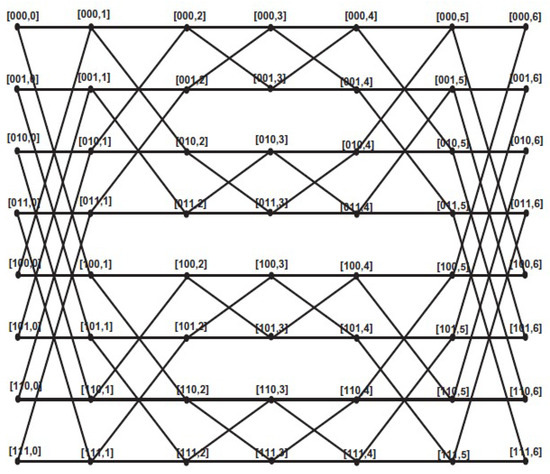
Figure 1.
Graph corresponding to .
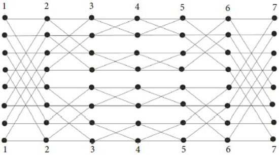
Figure 2.
Graph corresponding to .
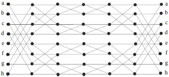
Figure 3.
Graph corresponding to .
2. Motivation, Proposed Problem and Organization
The network analysis theory has made contributions in many areas, such as thermal transport [40], cetane number prediction [41], AI for supply chains [42], and anticipating and building public policy through social networks [43]. Measuring entropy is among the most researched scientific topics because of its capacity to reveal both an object’s certainty and uncertainty. In light of the significance of ICNs, we therefore propose to use entropy measurements to extract structure-based information. Thus, between the general introduction of the subject and the technical findings of the manuscript, we explicitly state the objectives of this manuscript along with its organization. A recent study on the interconnection networks mentioned before, with a strong foundation in topological indices, entropy measures and complexity analysis, appeared in [28]. The topic was not completely resolved, though, and in [28], possible problems were identified, including using other topological indices to define new information functionals and examining entropy measures obtained from these new functionals to understand the complexity of these interconnection networks. In this paper, we investigate the aforementioned problem from [28], while simultaneously considering the advantage of the substantial impact of the topological indices (TIs) from [44,45,46,47]. It is achieved by computing their entropy measures, whereas the entropy measures are based on information functionals. These information functionals are defined through well-established and vastly studied notions of topological indices. The paper is structured into three more sections. The necessary materials and the designed methodology are explained in the next section. In Section 4, we determine the analytical formulae for the entropy measures obtained via new information functionals. In Section 5, we present the complexity analysis through our results by using numeric data and graphical tools. At the end, we discuss the advantages and limitations of the proposed model, along with a possible future work direction.
3. Materials and Methods
The focus of this section is to review some fundamental notions to study the complexity of the networks via degree-based entropy measures. Let G be a graph with and as the vertex set and the edge set, respectively. For any , the notations and represent the degree of v and the sum of the degrees of all adjacent vertices to v, i.e., . In Table 1, some degree-dependent TIs are listed, which are further used to compute the entropy measures including the first, second and third redefined Zagreb entropy , the fourth atom-bond connectivity entropy , the fifth geometric arithmetic entropy and the Sanskruti entropy given in Table 2.

Table 1.
Degree-dependent TIs.
Table 2.
Degree-dependent entropies.
The definition of the entropy of an edge-weighted graph was introduced by Chen et al. [35], where and represent the vertex set, the edge set and the edge weight of an edge , respectively. This is defined as:
Other entropies using particular edge weight in Equation (1) that were discovered and mathematically formulated in [24] are given in Table 2.
In this article, we analyze the complexity of , and via several degree-dependent entropy measures given in Table 2. In first step, we derive analytic formulae for TIs, which are further utilized in computing respective entropy measures by using an edge partition scheme. In the second step, we give a numerical and graphical comparison of these networks for clearer comprehension of their structural information. The concluding remarks are given at the end.
4. Main Results
The current section is devoted to main findings of the manuscript and is divided into three subsections, each one for , and .
4.1. Entropy Measures Obtained via Degree-Based Topological Indices for Benes Network
In , among vertices and vertices are of degree 4 and degree 2, respectively. The cardinality of the edge set is . The partitions of are given in Table 3 and Table 4. The notation represents the set of all edges with .
Table 3.
Edge partition of based on the degree of end vertices.
Table 4.
Edge partition of based on of end vertices.
For next entropy measures, we now develop an edge partition of based on of end vertices in the following table. Recall that .
Theorem 1.
For with , we have
Proof.
- By using Table 3, we compute the first redefined Zagreb index asBy using the above calculated index and Table 3, we obtain the first redefined Zagreb entropy as
- By using Table 4, we obtain the fourth atom-bond connectivity index asBy using the above-calculated index and Table 4, we obtain the fourth atom-bond connectivity entropy as
4.2. Entropy Measures Obtained via Degree-Based Topological Indices for
In an -dimensional horizontal cylindrical representation of a Benes network , we have and . The edge partition based on the degree of end vertices is developed in the table given next. We use this partition to obtain the precise representations of the entropies by computing the corresponding TIs for each one.
Next, we develop an edge partition table of and compute further entropy measures for . This partition is based on of end vertices. Recall that .
Theorem 2.
For with in and in , we have
Proof.
Table 6.
Edge partition of (for ) based on degree sum of end vertices.
Table 6.
Edge partition of (for ) based on degree sum of end vertices.
| , | Frequency |
|---|---|
| 8 | |
| 4 | |
| 4 | |
| 8 | |
| 4 | |
| 8 | |
| 4 | |
| 2 | |
| 4 | |
| 4 | |
| 4 | |
| 4 | |
| 2 | |
4.3. Entropy Measures Obtained via Degree-Based Topological Indices for
In an -dimensional vertical cylindrical representation of a Benes network , we have and . By observation, we note that each vertex of has degree 4. As all the vertices of have same degree 4, therefore, for each . So, all edges of have same degree 4 of end vertices, and thus, the partition of edge set of contains all its edges in one class. Similarly, the values of for each implies partition of the edge set of containing all its edges in one class. By utilizing these facts in the formulae of the entropies given in Table 2, we obtain the following formulae of entropy measures for .
Theorem 3.
For , we have
- =
5. Complexity-Based Classification of Interconnection Networks via Entropy Measures by Using Numeric Tables and Graphical Analysis
In this sections, we apply the proved results of this manuscript to classify the studied interconnection networks in terms their complexity measures. We construct numerical tables by taking specific values of the parameter . In Table 7, we consider the values of and find the corresponding values of the TIs for , and . Secondly, in Table 8, we consider the values of and find the corresponding values of the entropies for , and . Table 8 assists in understanding and comparing the entropy and consequently the complexity measures of the studied network. Note that the higher the value of entropy, the complex the networks, and vice versa. Also, remember that not all topological indices or entropy measures describe all the network property. Thus, our method will assist in filtering those topological indices that provide a certain conclusion about the complexity measures of these networks. As a comparison, we start with the entropy measure corresponding the TI , denoted by . The values of the entropy measures for are greater than both and , which shows that both horizontal and vertical identifications in Benes networks help to reduce its complexity. However, while observing the case , different results are obtained. In this case, the behaviour is opposite to the previous one. It can be interpreted as both the horizontal and vertical identifications resulting in an increase in the complexity of the Benes network. In terms of structure, it can be expressed that due to identifications, the degrees of certain vertices are increased, thus resulting in a more complex network. Similarly, the other entropy measures can also be compared. The most interesting observation among the entropy/complexity comparison is that as the value of is increasing, the difference between the entropy measures is reducing, which in fact is a true description of the structure. Because all three types of networks have the same interior, the differences appear on the boundary and the neighbors of the boundary. Thus, an increase in the value of results in a higher increase in the interior (compared to the boundary). Therefore, the entropy and complexity difference keeps on reducing. This comparison and behavior are also expressed using Figure 4, Figure 5 and Figure 6.
Table 7.
Numerical values of degree-dependent TIs for , and .
Table 8.
Numerical values of degree-dependent entropies for , and .
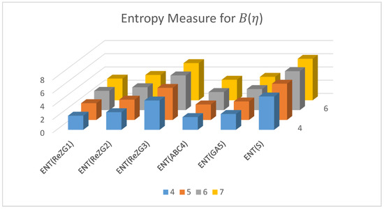
Figure 4.
The graphical representation of trends of entropy measures of with .
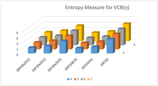
Figure 5.
The graphical representation of trends of entropies of with .
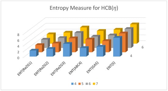
Figure 6.
The graphical representation of trends of entropies of with .
6. Conclusions and Future Work
In [6,11], a comprehensive and fruitful discussion was performed on the frequency of research on numeric parameters associated to graphs. It was also emphasized that associating numeric values to the graphs via complex computation is not sufficient, as it does not add value to the field. In our work, we have established a model through entropy measures which are based on information functionals, which helps in determining the complexity of networks. In the first step, the general formulae of entropy measures corresponding to any value of the parameter are given, which provides the rigorous base of the study. However, as per the standards set in [6,11], it is important to deduce numeric data and analyze which applications the proved results provide. In the previous section, we presented that the numeric data provide obvious patterns in cases of few defined entropies. However, in few cases, the patterns are reversed or no pattern is observed. But, as a limitation of this research direction, it is also discussed in [6,11] that one numeric parameter associated is not necessarily applicable to all properties, which in fact is a basic reason for the introduction of so many numeric parameters of the graphs. Thus, the patterns obtained in the previous sections justify the usefulness of entropy measures. However, the values that are not providing the same entropy patters or no pattern cannot be discarded, and this is a limitation of the model. Thus, it raise natural questions about whether we can introduce a family of entropy measures that completely distinguish these networks through same pattern of numeric values. In future, the current model can also be implemented on other related families of networks or isomers for discrimination.
Author Contributions
Conceptualization, J.Z. and A.F.; methodology, M.M. and A.R.; validation, A.F. and M.M.; investigation, A.F. and M.M.; writing—original draft preparation, J.Z., M.M. and A.R.; writing—review and editing, A.F. and J.Z.; visualization, J.Z.; supervision, A.F.; project administration, J.Z.; funding acquisition, J.Z. All authors have read and agreed to the published version of the manuscript.
Funding
The Major Research Foundation of Educational Reform of Anhui Provincial Education Department (2021zdjgxm025); The Major Science Research Program of Anhui Provincial Education Department(2022AH040048).
Institutional Review Board Statement
Not applicable.
Informed Consent Statement
Not applicable.
Data Availability Statement
Not applicable.
Acknowledgments
All the authors are thankful to their respective institutes. In addition, Asfand Fahad also acknowledges the Grant No. YS304023966 to support his Postdoctoral Fellowship at Zhejiang Normal University, China.
Conflicts of Interest
The authors declare no conflict of interest.
References
- Shang, Y. Sombor index and degree-related properties of simplicial networks. Appl. Math. Comput. 2022, 419, 126881. [Google Scholar] [CrossRef]
- Liu, J.B.; Bao, Y.; Zheng, W.T. Analyses of some structural properties on a class of hierarchical scale-free networks. Fractals 2022, 30, 2250136. [Google Scholar] [CrossRef]
- Azeem, M.; Jamil, M.K.; Shang, Y. Notes on the localization of generalized hexagonal cellular networks. Mathematics 2023, 11, 844. [Google Scholar] [CrossRef]
- Liu, J.B.; Bao, Y.; Zheng, W.T.; Hayat, S. Network coherence analysis on a family of nested weighted n-polygon networks. Fractals 2021, 29, 2150260. [Google Scholar] [CrossRef]
- Aguilar-Sanchez, R.; Mendez-Bermudez, J.A.; Rodriguez, J.M.; Sigarreta, J.M. Normalized Sombor indices as complexity measures of random networks. Entropy 2021, 23, 976. [Google Scholar] [CrossRef] [PubMed]
- Das, K.C.; Mondal, S. On neighborhood inverse sum indeg index of molecular graphs with chemical significance. Inf. Sci. 2023, 623, 112–131. [Google Scholar] [CrossRef]
- Ramane, H.S.; Yalnaik, A.S. Status connectivity indices of graphs and its applications to the boiling point of benzenoid hydrocarbons. J. Appl. Math. Comput. 2017, 55, 609–627. [Google Scholar] [CrossRef]
- Selvakumar, K.; Gangaeswari, P.; Arunkumar, G. The Wiener index of the zero-divisor graph of a finite commutative ring with unity. Discret. Appl. Math. 2022, 311, 72–84. [Google Scholar] [CrossRef]
- Chai, C.; Lu, G.; Wang, R.; Lyu, C.; Lyu, L.; Zhang, P.; Liu, H. Graph-based structural difference analysis for video summarization. Inf. Sci. 2021, 577, 483–509. [Google Scholar] [CrossRef]
- Li, H.; Cao, J.; Zhu, J.; Liu, Y.; Zhu, Q.; Wu, G. Curvature graph neural network. Inf. Sci. 2022, 592, 50–66. [Google Scholar] [CrossRef]
- Ma, Y.; Dehmer, M.; Kuzni, U.; Tripathi, S.; Ghorbani, M.; Tao, J.; Emmert-Streib, F. The usefulness of topological indices. Inf. Sci. 2022, 606, 143–151. [Google Scholar] [CrossRef]
- Liu, J.B.; Pan, X.F. Minimizing Kirchhoff index among graphs with a given vertex bipartiteness. Appl. Math. Comput. 2016, 291, 84–88. [Google Scholar] [CrossRef]
- Das, K.C.; Vetrik, T. General Gutman index of a graph. MATCH Commun. Math. Comput. Chem. 2023, 89, 583–603. [Google Scholar] [CrossRef]
- Liu, J.B.; Gu, J.J.; Wang, K. The expected values for the Gutman index, Schultz index, and some Sombor indices of a random cyclooctane chain. Int. J. Quantum Chem. 2023, 123, e27022. [Google Scholar] [CrossRef]
- Das, K.C.; Elumalai, S.; Balachandran, S. Open problems on the exponential vertex-degree-based topological indices of graphs. Discret. Appl. Math. 2021, 293, 38–49. [Google Scholar] [CrossRef]
- Wiener, H. Structural determination of paraffin boiling points. J. Am. Chem. Soc. 1947, 69, 17–20. [Google Scholar] [CrossRef]
- Randic, M. Characterization of molecular branching. J. Am. Chem. Soc. 1975, 97, 6609–6615. [Google Scholar] [CrossRef]
- Poulik, S.; Ghorai, G. Determination of journeys order based on graph’s Wiener absolute index with bipolar fuzzy information. Inf. Sci. 2021, 545, 608–619. [Google Scholar] [CrossRef]
- Poulik, S.; Ghorai, G. Estimation of most effected cycles and busiest network route based on complexity function of graph in fuzzy environment. Artif. Intell. Rev. 2022, 55, 4557–4574. [Google Scholar] [CrossRef]
- Shannon, C.E. A mathematical theory of communication. Bell Syst. Tech. J. 1948, 27, 379–423. [Google Scholar] [CrossRef]
- Rashevsky, N. Life, information theory, and topology. Bull. Math. Biophys. 1955, 17, 229–235. [Google Scholar] [CrossRef]
- Dehmer, M.; Grabner, M. The discrimination power of molecular identification numbers revisited. MATCH Commun. Math. Comput. Chem. 2013, 69, 785–794. [Google Scholar]
- Ulanowicz, R.E. Quantitative methods for ecological network analysis. Comput. Biol. Chem. 2004, 28, 321–339. [Google Scholar] [CrossRef] [PubMed]
- Manzoor, S.; Siddiqui, M.K.; Ahmad, S. On entropy measures of molecular graphs using topological indices. Arab. J. Chem. 2020, 13, 6285–6298. [Google Scholar] [CrossRef]
- Zhong, J.; Han, C.; Zhang, X.; Chen, P.; Liu, R. scGET: Predicting cell fate transition during early embryonic development by single-cell graph entropy. Genom. Proteom. Bioinform. 2021, 19, 461–474. [Google Scholar] [CrossRef]
- Hui, Z.H.; Fahad, A.; Qureshi, M.I.; Irfan, R.; Shireen, A.; Iqbal, Z.; Alyusufi, R. On Entropy Measures and Eccentricity-Based Descriptors of Polyamidoamine (PAMAM) Dendrimers. J. Chem. 2022, 2022, 1214137. [Google Scholar] [CrossRef]
- Omar, Y.M.; Plapper, P. A survey of information entropy metrics for complex networks. Entropy 2020, 22, 1417. [Google Scholar] [CrossRef] [PubMed]
- Yang, J.; Fahad, A.; Mukhtar, M.; Anees, M.; Shahzad, A.; Iqbal, Z. Complexity Analysis of Benes Network and Its Derived Classes via Information Functional Based Entropies. Symmetry 2023, 15, 761. [Google Scholar] [CrossRef]
- Sabirov, D.S.; Shepelevich, I.S. Information entropy in chemistry: An overview. Entropy 2021, 23, 1240. [Google Scholar] [CrossRef]
- Mowshowitz, A.; Dehmer, M. Entropy and the complexity of graphs revisited. Entropy 2012, 14, 559–570. [Google Scholar] [CrossRef]
- Cao, S.; Dehmer, M.; Shi, Y. Extremality of degree-based graph entropies. Inf. Sci. 2014, 278, 22–33. [Google Scholar] [CrossRef]
- Cao, S.; Dehmer, M. Degree-based entropies of networks revisited. Appl. Math. Comput. 2015, 261, 141–147. [Google Scholar] [CrossRef]
- Dehmer, M. Information processing in complex networks: Graph entropy and information functionals. Appl. Math. Comput. 2008, 201, 82–94. [Google Scholar] [CrossRef]
- Dehmer, M.; Sivakumar, L.; Varmuza, K. Uniquely discriminating molecular structures using novel eigenvalue-based descriptors. Match-Commun. Math. Comput. Chem. 2012, 67, 147–172. [Google Scholar]
- Chen, Z.; Dehmer, M.; Shi, Y. A note on distance-based graph entropies. Entropy 2014, 16, 5416–5427. [Google Scholar] [CrossRef]
- Hussain, A.; Numan, M.; Naz, N.; Butt, S.I.; Aslam, A.; Fahad, A. On topological indices for new classes of benes network. J. Math. 2021, 2021, 6690053. [Google Scholar] [CrossRef]
- Imran, M.; Hayat, S.; Mailk, M.Y.H. On topological indices of certain interconnection networks. Appl. Math. Comput. 2014, 244, 936–951. [Google Scholar] [CrossRef]
- Wang, W.; Nisar, A.; Fahad, A.; Qureshi, M.I.; Alameri, A. Modified Zagreb connection indices for benes network and related classes. J. Math. 2022, 2022, 8547332. [Google Scholar] [CrossRef]
- Wang, W.; Arshad, H.; Fahad, A.; Javaid, I. On Some Ev-Degree and Ve-Degree Dependent Indices of Benes Network and Its Derived Classes. Comput. Model. Eng. Sci. 2023, 135, 1685–1699. [Google Scholar]
- Jiang, S.; Landen, O.L.; Whitley, H.D.; Hamel, S.; London, R.; Clark, D.S.; Sterne, P.; Hansen, S.B.; Hu, S.X.; Collins, G.W.; et al. Thermal transport in warm dense matter revealed by refraction-enhanced X-ray radiography with a deep-neural-network analysis. Commun. Phys. 2023, 6, 98. [Google Scholar] [CrossRef]
- Kim, Y.; Cho, J.; Naser, N.; Kumar, S.; Jeong, K.; McCormick, R.L.; John, P.C.S.; Kim, S. Physics-informed graph neural networks for predicting cetane number with systematic data quality analysis. Proc. Combust. Inst. 2023, 39, 4969–4978. [Google Scholar] [CrossRef]
- Maghsoudi, M.; Shokouhyar, S.; Ataei, A.; Ahmadi, S.; Shokoohyar, S. Co-authorship network analysis of AI applications in sustainable supply chains: Key players and themes. J. Clean. Prod. 2023, 422, 138472. [Google Scholar] [CrossRef]
- Zhang, W.; Zhang, M.; Yuan, L.; Fan, F. Social network analysis and public policy: What’s new? J. Asian Public Policy 2023, 16, 115–145. [Google Scholar] [CrossRef]
- Ranjini, P.S.; Lokesha, V.; Usha, A. Relation between phenylene and hexagonal squeeze using harmonic index. Int. J. Graph Theory 2013, 1, 116–121. [Google Scholar]
- Ghorbani, M.; Hosseinzadeh, M.A. Computing ABC4 index of nanostar dendrimers. Optoelectron. Adv. Mater.-Rapid Commun. 2010, 4, 1419–1422. [Google Scholar]
- Graovac, A.; Ghorbani, M.; Hosseinzadeh, M.A. Computing fifth geometric-arithmetic index for nanostar dendrimers. J. Discret. Math. Its Appl. 2011, 1, 33–42. [Google Scholar]
- Hosamani, S.M. Computing Sanskruti index of certain nanostructures. J. Appl. Math. Comput. 2017, 54, 425–433. [Google Scholar] [CrossRef]
Disclaimer/Publisher’s Note: The statements, opinions and data contained in all publications are solely those of the individual author(s) and contributor(s) and not of MDPI and/or the editor(s). MDPI and/or the editor(s) disclaim responsibility for any injury to people or property resulting from any ideas, methods, instructions or products referred to in the content. |
© 2023 by the authors. Licensee MDPI, Basel, Switzerland. This article is an open access article distributed under the terms and conditions of the Creative Commons Attribution (CC BY) license (https://creativecommons.org/licenses/by/4.0/).