SIMEX Estimation of Partially Linear Multiplicative Regression Model with Mismeasured Covariates

Abstract

In many practical applications, such as the studies of financial and biomedical data, the response variable usually is positive, and the commonly used criteria are based on absolute errors, which is not desirable. Rather, the relative errors are more of concern. We consider statistical inference for a partially linear multiplicative regression model when covariates in the linear part are measured with error. The simulation–extrapolation (SIMEX) estimators of parameters of interest are proposed based on the least product relative error criterion and B-spline approximation, where two kinds of relative errors are both introduced and the symmetry emerges in the loss function. Extensive simulation studies are conducted and the results show that the proposed method can effectively eliminate the bias caused by the measurement errors. Under some mild conditions, the asymptotic normality of the proposed estimator is established. Finally, a real example is analyzed to illustrate the practical use of our proposed method.

1. Introduction

In many applications, such as studies on financial and biomedical data, the response variable is usually positive. For modeling the relationship between the positive response and a set of explanatory variables, the natural idea is to first take an appropriate transformation for the response, e.g., the logarithmic transformation, and then, some common regression models, such as linear regression or quantile regression, which can be employed based on the transformed data. As argued by [1], the least-squares or least absolute deviation criteria are both based on absolute errors, which is not desirable in many practical applications. Rather, the relative errors are more of concern.

In the early literature, many authors contributed fruitfully to this issue; see [2,3,4], where the relative error is defined as the ratio of the error relative to the target value. Since the work of [1], where both the ratios of the error relative to both the target value and the predictor are introduced in the loss function, called the least absolute relative error (LARE) criterion, more attention has been focused on the multiplicative regression (MR) model, and various extensions have been investigated. For example, Ref. [5] considered the estimation problem of the nonparametric MR model; see also [6,7] and references therein. In particular, some semi-parametric MR models have been studied. When estimating the nonparametric function $g\left(z\right)$ in these models, such as the partially linear MR model ([8,9,10]), single-index MR model ([11,12,13]), varying-coefficient MR model ([14]), and others ([15]), almost all researchers use the local linear smoothing technique and approximate it in a neighborhood of z for obtaining its estimation, where a good choice of the bandwidths is quietly critical and its value is possibly sensitive to the performance of the resulting estimation and inference. Additionally, due to the fact that the value of the function at every observation of z is estimated separately, the optimal selection of bandwidth for all observations may be not the same. Thus, the computation is cumbersome and the numerical problem becomes untractable when the sample size is large. As a result, researchers have had to compromise and assume that the bandwidths used for estimating the nonparametric function are the same.

When solving nonparametric regression, spline-based methods, such as regression splines, smoothing splines, and penalized splines, are popular and applied extensively in many fields. Recently, Ref. [16] proposed multiplicative additive models based on the least product relative error criterion (LPRE), where the B-spline basis functions are used to estimate the nonparametric functions. Simulation studies have demonstrated that their approach performs well. It is worth noting that the loss function based on LPRE is smooth enough and differentiable with respect to the regression parameter, in contrast to that based on LARE. Moreover, LPRE inherits the symmetry between the two kinds of relative errors presented in LARE. Using this symmetry makes the computation and derivation of asymptotic properties easier.

A common feature in the above-mentioned literature is that these studies presume that all variables in the model are precisely observed. However, in many applications, some covariates cannot be measured exactly due to various limitations; see [17] for such examples in econometric, biology, nutrition, and toxicology studies. Extensive studies have been conducted, such as quantile and other traditional robust statistical inference procedures in the measurement error setup. Only recently have we witnessed an interest in applying multiplicative regression when the covariates are contaminated with measurement errors. Ref. [18] developed a simulation–extrapolation (SIMEX) estimation method for unknown parameters based on the LPRE criterion for the linear and varying coefficient multiplicative models, respectively, with the covariates being measured with additive error, where the measurement error is assumed to follow a normal distribution, and under certain conditions, the large sample properties of the given estimates are proved.

The SIMEX estimation procedure was first developed by [19] to reduce the estimation bias in the presence of additive measurement errors. Since then, the SIMEX method has gained more attention in the literature, and it has become a standard tool for analyzing complex regression models. A significant feature of SIMEX is that one can rely on standard inferential procedures to estimate the unknown parameters. Since its conception, more researchers have extended the SIMEX method to various applications. Ref. [20] considered statistical inference for additive partial linear models when the linear covariate is measured with error using attenuation-to-correction and SIMEX methods. Ref. [21] proposed graphical proportional hazards measurement error models and developed SIMEX procedures for the parameter of interest with complex structured covariates. To the best of our knowledge, there are seldom studies on the partially linear multiplicative regression model with measurement error. To fill this gap, we will address this problem in detail in this paper.

This paper is organized as follows. In Section 2, we first introduce in detail the simulation–extrapolation method for the partially linear multiplicative regression model with measurement errors. Combining the B-spline approximation and the LPRE criterion, a new estimation method is proposed, and some remarks about the selection of number and location of knots and the asymptotic properties of the proposed estimator are presented. Some simulation studies are carried out to assess the performance of our method under a finite-sample situation in Section 3. A real example is analyzed to illustrate the practical usage of our proposed method in Section 4. Finally, some discussions in Section 5 conclude the paper.

2. Methodology

In this section, we propose the simulation–extrapolation estimation for regression parameters and the nonparametric function in the partially linear multiplicative regression model, where the covariates in the parametric part are measured with additive measurement errors. Computation details are presented, and some asymptotic results are also established.

2.1. Notations and Model

Let Y denote the positive response variable, which satisfies the following partially linear multiplicative regression model

$$Y=exp(X^{\top }\beta +g\left(Z\right))ϵ,$$

(1)

where X is the p-dimensional vector of covariates associated with the regression parameter vector $\beta$, Z is a continuous univariate variable, $ϵ$ is the positive error and independent of $(X,Z)$, and $g(.)$ is an unknown smooth link function.

Due to some practical limitations, the covariate X cannot be observed precisely. Instead, its surrogate, W, through the additive covariate measurement error structure

$$W=X+U,$$

(2)

is available, where U is the measurement error with mean zero and the covariance matrix ${\sum }_u$ and independent of $(X,Z)$ and $ϵ$. Assume that ${\sum }_u$ is known; otherwise, it can be estimated through the replication experiments technique, as argued in much of the literature such as [17]. When some components of X are error-free, the corresponding terms in ${\sum }_u$ are set to be zero. In particular, when ${\sum }_u$ is a zero matrix, i.e., U is zero, there is no measurement error.

We combine Models (1) and (2) and refer to it as the partially linear multiplicative regression measurement error (PLMR-ME) model. Let $(Y_i,X_i,Z_i,W_i)$$i=1,\dots ,n$ be independent and identical replicates of $(Y,X,Z,W)$.

2.2. SIMEX Estimation of PLMR-ME Model

In general, the SIMEX method consists of a simulation step, an estimation step, and an extrapolation step. Before the detailed introduction of our method, we must specify two kinds of parameters; one is the simulation times, denoted by $n_0$, and the other is the levels of added error, denoted by $\lambda \in \mathsf{\Lambda }=\{{\lambda }_1,\dots ,{\lambda }_M\}$. Oftentimes, equally spaced values with ${\lambda }_1=0$ and ${\lambda }_M=2$ are adopted, M ranges from 10 to 20, and B is a given integer lying in [50,200].

In our method, we use the SIMEX algorithm, B-spline approximation, and the LPRE criterion to estimate $\beta$ and $g(.)$. First, we approximate $g(.)$ using a B-spline function, i.e., $g\left(z\right)\approx {\sum }_{j=1}^{K_n}{\alpha }_j{B}_j\left(z\right)$, where $B_j(.)$ is the B-spline basis function of order d with $k_n$ internal knots, and $K_n=d+k_n$. Then, Model (1), as in [22,23], can be rewritten as the spline model

$$Y=exp(X^{\top }\beta +B^{\top }\alpha )\epsilon ,$$

where $B=B\left(Z\right)={(B_1\left(Z\right),\dots ,B_{K_n}\left(Z\right))}^{\top }$, $\alpha ={({\alpha }_1,\dots ,{\alpha }_{K_n})}^{\top }$ is the corresponding vector of the spline coefficients. In this way, the estimation problem of unknown function $g(.)$ is transformed into the estimation of $\alpha$. Next, we employ the LPRE criterion to estimate $\beta$ and $\alpha$. Explicitly speaking, the proposed SIMEX algorithm proceeds as follows.

(1)

Simulation step.

For each $\lambda \in \mathsf{\Lambda }$, generate B independent random samples of size n from $N(0,{\sum }_u)$. That is to say, for the j-th sample, generate a sequence of pseudo-predictors

$$W_{ib}\left(\lambda \right)=W_i+\sqrt{\lambda }{V}_{ib},i=1,\dots ,n,b=1,\dots ,n_0,$$

where $V_{ib}\sim N(0,{\sum }_u)$. Note that the covariance matrix of $W_{ib}\left(\lambda \right)$ given $X_i$ is

$$Var\left(W_{ib}\left(\lambda \right)\right|X_i)=\lambda {\sum }_u+Var\left(W_i\right|X_i)=(1+\lambda ){\sum }_u.$$

Thus, when $\lambda =-1$, it follows that $Var\left(W_{ij}\left(\lambda \right)\right|X_i)=0$. Combining the fact that $E\left(W_{ib}\left(\lambda \right)\right|X_i)=X_i$, the conditional mean square error of $W_{ib}\left(\lambda \right)$, defined as $E\left[{(W_{ib}\left(\lambda \right)-X_i)}^2\right|X_i]$, converges to zero as $\lambda \to -1$.

(2)

Estimation step.

For a fixed $\lambda$, based on the b-th random sample $(Y_i,W_{ib}\left(\lambda \right),Z_i)$ $i=1,\dots ,n$, one can obtain the estimator of $(\beta ,\alpha )$, denoted by $({\widehat{\beta }}_b\left(\lambda \right),{\widehat{\alpha }}_b\left(\lambda \right))$, which is the minimizer of the objective function

$$\begin{array}{ccc}\hfill L_{nb}(\beta ,\alpha ;\lambda )& =& \hfill \sum _{i=1}^n\left\{\left|\frac{Y_i-exp(W_{ib}^{\top }\left(\lambda \right)\beta +B_i^{\top }\alpha )}{Y_i}\right|\times \left|\frac{Y_i-exp(W_{ib}^{\top }\left(\lambda \right)\beta +B_i^{\top }\alpha )}{exp(W_{ib}^{\top }\left(\lambda \right)\beta +B_i^{\top }\alpha )}\right|\right\}\hfill \\ & =& \hfill \sum _{i=1}^n\left[Y_{i}exp(-W_{ib}^{\top }\left(\lambda \right)\beta -B_i^{\top }\alpha )+Y_i^{-1}exp(W_{ib}^{\top }\left(\lambda \right)\beta +B_i^{\top }\alpha )-2\right],\hfill \end{array}$$

where $B_i=B\left(Z_i\right)$. Then, define the final estimates of $(\beta ,\alpha )$ using the average of $({\widehat{\beta }}_b\left(\lambda \right),{\widehat{\alpha }}_b\left(\lambda \right))$ over $b=1,\dots ,n_0$, defined by $\widehat{\beta }\left(\lambda \right)={\sum }_{b=1}^{n_0}{\widehat{\beta }}_b\left(\lambda \right)/n_0$ and $\widehat{\alpha }\left(\lambda \right)={\sum }_{b=1}^{n_0}{\widehat{\alpha }}_b\left(\lambda \right)/n_0$, where $\lambda \in \mathsf{\Lambda }$. Furthermore, the corresponding estimator of $g\left(z\right) is$$\widehat{g}(z;\lambda )=B^{\top }\widehat{\alpha }\left(\lambda \right)$.

(3)

Extrapolation step.

Consider two extrapolation models: linear and quadratic. Without loss of generality, denote the extrapolation function by $\mathsf{\Psi }(\lambda ,\mathsf{\Gamma })$, where $\mathsf{\Gamma }$ is the regression parameter vector. At this time, the linear extrapolation function is $\mathsf{\Psi }(\lambda ,\mathsf{\Gamma })={\gamma }_0+{\gamma }_1\lambda$, and the quadratic one is $\mathsf{\Psi }(\lambda ,\mathsf{\Gamma })={\gamma }_0+{\gamma }_1\lambda +{\gamma }_1{\lambda }^2$. For the two sequences $\{(\lambda ,\widehat{\beta }\left(\lambda \right)),\lambda \in \mathsf{\Lambda }\}$ and $\{(\lambda ,\widehat{g}(z;\lambda )),\lambda \in \mathsf{\Lambda }\}$, we fit a regression model to each of the two sequences from

$$\widehat{\beta }\left(\lambda \right)={\mathsf{\Psi }}_1(\lambda ,{\mathsf{\Gamma }}_1)+{\epsilon }_1,\widehat{g}(z;\lambda )={\mathsf{\Psi }}_2(\lambda ,{\mathsf{\Gamma }}_2)+{\epsilon }_2$$

respectively, where ${\epsilon }_1$ and ${\epsilon }_2$ are random errors. Using the least-squares method, one can obtain the estimates of ${\mathsf{\Gamma }}_1$ and ${\mathsf{\Gamma }}_2$ and denote them as ${\widehat{\mathsf{\Gamma }}}_1$ and ${\widehat{\mathsf{\Gamma }}}_2$, respectively. Then, the SIMEX estimator of $\beta$ is defined as the predicted value

$${\widehat{\beta }}_{SIMEX}={\mathsf{\Psi }}_1(-1,{\widehat{\mathsf{\Gamma }}}_1).$$

Meanwhile, the naive estimator of $\beta$ reduces to ${\mathsf{\Psi }}_1(0,{\widehat{\mathsf{\Gamma }}}_1)$. As for $\beta$ above, the nonparametric term $g(.)$ can be estimated in the same way. Denote the SIMEX estimator of $g\left(z\right)$ by ${\widehat{g}}_{SIMEX}\left(z\right)={\mathsf{\Psi }}_2(-1,{\widehat{\mathsf{\Gamma }}}_2)$.

2.3. Asymptotic Results

To derive the asymptotic normality of the SIMEX estimator ${\widehat{\beta }}_{SIMEX}$, some regularity conditions are necessary to be introduced as follows.

(A1)

$E\left[(ϵ-{ϵ}^{-1})\right|X,Z]=0$.

(A2)

$E\left(X{X}^{\top }\right)$ is a positive definite matrix.

(A3)

There exists $\delta >0$ such that $E[(ϵ+{ϵ}^{-1})exp\left(\delta \right|\left|X\right|\left|\right)]<\infty$, $E[{(ϵ+{ϵ}^{-1})}^{2}exp\left(\delta \right|\left|X\right|\left|\right)]<\infty$, and $E[{(ϵ+{ϵ}^{-1})}^2{\left(x_j{x}_k{x}_l\right)}^{2}exp\left(\delta \right|\left|X\right|\left|\right)]<\infty ,j,k,l=1,\dots ,p$.

(A4)

$g(.)\in \mathcal{H}=\{g\in C^r[a,b]:\Vert g^{\left(j\right)}{\Vert }_{\infty }\le M_0,j=1,\dots ,r,|g^{\left(r\right)}\left(z_1\right)-g^{\left(r\right)}\left(z_2\right)|\le M_1|z_1-z_2\left|\right\}$, where $M_0$ and $M_1$ are some positive constants and ${\Vert ·\Vert }_{\infty }$ is the superior norm. $0\le r\le d$.

Conditions (A1)–(A3) are common requirements in the penalized spline theory. (A4) is the regularization condition used in the study of MR. (A5) is an identification condition for the LPRE estimation, which is similar to the zero-mean condition in the classical linear mean regression.

Before presenting our result, some notations need to be introduced in advance. Let $\widehat{\beta }\left(\mathsf{\Lambda }\right)=(\widehat{\beta }{\left({\lambda }_1\right)}^{\top },\dots ,\widehat{\beta }{\left({\lambda }_M\right)}^{\top })$ and $\mathsf{\Gamma }={({\mathsf{\Gamma }}_{11}^{\top },\dots ,{\mathsf{\Gamma }}_{1p}^{\top })}^{\top }$, where ${\mathsf{\Gamma }}_{1j}^{\top }$ is the true parameter vector estimated in the extrapolation step for the j-th component of $\widehat{\beta }\left(\lambda \right)$. Define $G({\lambda }_k,\mathsf{\Gamma })=(\mathsf{\Psi }({\lambda }_k,{\mathsf{\Gamma }}_{11}),\dots ,\mathsf{\Psi }({\lambda }_k,{\mathsf{\Gamma }}_{1p}))$ and $G(\mathsf{\Lambda },\mathsf{\Gamma })=(G({\lambda }_1,\mathsf{\Gamma }),\dots ,G({\lambda }_M,\mathsf{\Gamma }))$. Let $\widehat{\mathsf{\Gamma }}$ be the minimizer of $Res\left(\mathsf{\Gamma }\right)Res{\left(\mathsf{\Gamma }\right)}^{\top }$, where $Res\left(\mathsf{\Gamma }\right)=\widehat{\beta }\left(\mathsf{\Lambda }\right)-G(\mathsf{\Lambda },\mathsf{\Gamma })$. According to the least-squares theory, $\widehat{\mathsf{\Gamma }}$ satisfies $s\left(\mathsf{\Gamma }\right)Res\left(\mathsf{\Gamma }\right)=0$, where $s\left(\mathsf{\Gamma }\right)=\partial Res\left(\mathsf{\Gamma }\right)/\partial \left({\mathsf{\Gamma }}^{\top }\right)$. Denote $D\left(\mathsf{\Gamma }\right)=s\left(\mathsf{\Gamma }\right)s{\left(\mathsf{\Gamma }\right)}^{\top }$ and $\mathcal{G}(\lambda ,\mathsf{\Gamma })=\partial G(\lambda ,\mathsf{\Gamma })/\partial \left(\mathsf{\Gamma }\right)$.

Theorem 1.

Assume that the extrapolation function is theoretically exact. Under the conditions (A1)–(A4), it follows that as $n\to \infty$, we have

$$\sqrt{n}({\widehat{\beta }}_{SIMEX}-\beta ){\to }_{d}N(0,\mathcal{G}(-1,\mathsf{\Gamma })\sum \left(\mathsf{\Gamma }\right)\mathcal{G}{(-1,\mathsf{\Gamma })}^{\top }),$$

Proof. 

Assume that $\beta \left(\lambda \right)$ is the true value based on the model $Y_i=exp(W_{ib}{\left(\lambda \right)}^{\top }\beta +g\left(Z_i\right)){\widetilde{ϵ}}_i.$ Using the similar method in Theorem 2 in [16], we have

$$\sqrt{n}({\widehat{\beta }}_b\left(\lambda \right)-\beta \left(\lambda \right))=-\sqrt{n}{\left[K(\beta \left(\lambda \right),\lambda )\right]}^{-1}{J}_n(\beta \left(\lambda \right),\lambda )+o_P\left(1\right),$$

where

$$K(\beta \left(\lambda \right),\lambda )=E\left\{[Yexp(-W{\left(\lambda \right)}^{\top }\beta \left(\lambda \right)-g\left(Z\right))+Y^{-1}exp(W{\left(\lambda \right)}^{\top }\beta \left(\lambda \right)+g\left(Z\right))]W\left(\lambda \right)W_{ib}{\left(\lambda \right)}^{\top }\right\},$$

$$J_n(\beta \left(\lambda \right),\lambda )=\frac{1}{n}\left\{\sum _{i=1}^n[Y_{i}exp(-W_{ib}{\left(\lambda \right)}^{\top }\beta \left(\lambda \right)-g\left(Z_i\right))+Y_i^{-1}exp(W_{ib}{\left(\lambda \right)}^{\top }\beta \left(\lambda \right)+g\left(Z_i\right))]W_{ib}\left(\lambda \right)\right\},$$

and $W\left(\lambda \right)=X+\sqrt{\lambda }V$. Because $\widehat{\beta }\left(\lambda \right)={\sum }_{b=1}^{n_0}{\widehat{\beta }}_b\left(\lambda \right)/n_0$, it follows that

$$\sqrt{n}(\widehat{\beta }\left(\lambda \right)-\beta \left(\lambda \right))=-{\left[K(\beta \left(\lambda \right),\lambda )\right]}^{-1}{n}^{-1/2}{J}_{nB}(\beta \left(\lambda \right),\lambda )+o_P\left(1\right),$$

where $J_{nB}(\beta \left(\lambda \right),\lambda )=\frac{1}{n_0}{\sum }_{b=1}^{n_0}{\eta }_{ib}(\beta \left(\lambda \right),\lambda )=\frac{1}{n_0}{\sum }_{b=1}^{n_0}[Y_{i}exp(-W_{ib}{\left(\lambda \right)}^{\top }\beta \left(\lambda \right)-g\left(Z_i\right))+Y_i^{-1}exp(W_{ib}{\left(\lambda \right)}^{\top }\beta \left(\lambda \right)+g\left(Z_i\right))]W_{ib}\left(\lambda \right).$ Define $\sum \left(\lambda \right)=Cov\left(n^{-1/2}{J}_{nB}(\beta \left(\lambda \right),\lambda )\right)$. Some algebraic calculations show that

$$\sum \left(\lambda \right)=\frac{1}{n_0}Var\left({\eta }_{i1}(\beta \left(\lambda \right),\lambda )\right)+\frac{n_{0}2-n_0}{n_0^2}Cov({\eta }_{i1}(\beta \left(\lambda \right),\lambda ),{\eta }_{i2}(\beta \left(\lambda \right),\lambda )).$$

Then, according to the central limit theorem, it holds that

$$\sqrt{n}(\widehat{\beta }\left(\lambda \right)-\beta \left(\lambda \right)){\to }_{d}N(0,{\left[K(\beta \left(\lambda \right),\lambda )\right]}^{-1}\sum \left(\lambda \right)\left[K(\beta \left(\lambda \right),\lambda )\right]).$$

Write $\sum \left(\mathsf{\Lambda }\right)=diag(\sum \left({\lambda }_1\right),\dots ,\sum \left({\lambda }_M\right))$. In the following, using the standard derivation of the SIMEX method and the definition of $\widehat{\mathsf{\Gamma }}$, we have

$$\sqrt{n}(\widehat{\mathsf{\Gamma }}-\mathsf{\Gamma }){\to }_{d}N(0,\sum \left(\mathsf{\Gamma }\right)),$$

where $\sum \left(\mathsf{\Gamma }\right)=D{\left(\mathsf{\Gamma }\right)}^{-1}s\left(\mathsf{\Gamma }\right)\sum \left(\mathsf{\Lambda }\right)s{\left(\mathsf{\Gamma }\right)}^{\top }D{\left(\mathsf{\Gamma }\right)}^{-1}$. Finally, using the Delta method and noting the facts ${\widehat{\beta }}_{SIMEX}=\widehat{\beta }(-1)={\mathsf{\Psi }}_1(-1,\widehat{\mathsf{\Gamma }})$ and $\beta =\mathsf{\Psi }(-1,\mathsf{\Gamma })$, the desirable result is established. □

3. Simulation Studies

Numerical studies were conducted to evaluate the finite sample performance of our proposed SIMEX estimators under various situations. To fairly compare the SIMEX estimator with the naive estimator that ignores measurement errors and the true estimator based on the data without measurement errors, we set the degree of spline basis to be $q=2$ and the number of internal knots to $k_n=round\left(n^{1/3}\right)+1$; these are located on equally spaced quantiles for all methods. All results below are based on 500 replicates, where $M=11,{\lambda }_1=0,{\lambda }_2=0.2,\dots ,{\lambda }_M=2$, $n_0=50$, and the sample size $n=50$, 100, and 200, respectively. All simulations were implemented using the software R.

Now, generate $(Y_i,X_i,Z_i,W_i)$ from the following model

$$Y_i=exp({\beta }_1{X}_{1i}+{\beta }_2{X}_{2i}+sin\left(\frac{\pi Z_i}{2}\right)){ϵ}_i,W_i=X_i+U_i,i=1,\dots ,n,$$

where ${\beta }_1=1.5,{\beta }_2=-1$, $X_i=(X_{1i},X_{2i})$, $U_i=(U_{1i},U_{2i})$, $X_{1i}\sim N(0,1)$, $Z_{2i}\sim Binom(1,0.5)$, and $Z_i\sim Unif(-2,2)$ and is independent of the error ${ϵ}_i\sim exp\left(Unif(-2,2)\right)$. Further, we assume $U_{2i}=0$, which means that $X_{2i}$ is error-free. However, for $U_{1i}$, three measurement error distributions are considered, namely,

• Case 1: $U_{1i}\sim N(0,0.09)$;
• Case 2: $U_{1i}\sim N(0,0.36)$;
• Case 3: $U_{1i}\sim N(0,0.81)$.

These represent the light-level, moderate-level, and heavy-level measurement error, respectively. In the extrapolation step, consider both the linear and quadratic extrapolation functions and, respectively, denote the corresponding method as SIMEX1 and SIMEX2.

For estimators of $({\beta }_1,{\beta }_2)$, we record their empirical bias (BIAS), sample standard deviation (SD), and mean square error (MSE). For the nonparametric part, we use the averaged integrated absolute bias (IABIAS) and mean integrated square error (MISE), where for one estimator ${\widehat{g}}_j(j=1,\dots ,401)$, obtained from the j-th sample,

$$\mathrm{IABIAS}=\frac{1}{500}\sum _{j=1}^{500}\left[\frac{1}{ngrid}\sum _{k=1}^{ngrid}|{\widehat{g}}_j\left(u_k\right)-g\left(u_k\right)|\right],$$

$$\mathrm{MISE}=\frac{1}{500}\sum _{j=1}^{500}\left[\frac{1}{ngrid}\sum _{k=1}^{ngrid}{[{\widehat{g}}_j\left(u_k\right)-g\left(u_k\right)]}^2\right],$$

at the fixed grid points $\left\{u_k\right\}$ equally spaced in [−2,2] and $ngrid=401$. The values in parentheses below them are the associated sample standard deviation.

Table 1, Table 2 and Table 3 report the simulation results of different estimators of regression parameter and nonparametric function under cases 1–3 with different sample sizes. For ${\beta }_1$, we can see that when the measurement error is small as in Table 1, all methods behave similarly and the proposed SIMEX method gains no obvious advantage over the naive method. Not surprisingly, as the measurement error becomes moderate as seen in Table 2, the naive estimates are substantially biased and have a larger mean square error (MSE), while the SIMEX estimates, especially when the quadratic function is applied, are unbiased and have a smaller MSE. When the measurement error is large, as seen in Table 3, all methods except the true one are slightly biased, but the performance of the SIMEX methods is still relatively better than that of the naive method. For ${\beta }_2$ and $g(.)$, the corresponding covariates $X_{2i}$ and $Z_i$ are error-free, and it seems that under the same measurement error level and sample size, both the naive and SIMEX estimates have similar performance in terms of the sample standard deviation (SD) and MSE for ${\beta }_2$, integrated absolute bias (IABIAS), and mean integrated square error (MISE) for $g(.)$.

Table 1. Results for case 1 with different sample sizes $(\times {10}^{-2})$.

			${\mathit{\beta }}_1$				${\mathit{\beta }}_2$			$\mathit{g}(.)$
$\mathit{n}$	Method	BIAS	SD	MSE		BIAS	SD	MSE		IABIAS	MISE
50	True	−0.71	17.53	3.07		−2.02	31.73	10.09		39.71 (28.80)	12.63 (21.81)
	Naive	−1.87	17.69	3.15		−1.96	32.14	10.35		40.15 (29.46)	12.87 (21.97)
	SIMEX1	−0.68	17.82	3.17		−2.00	32.15	10.35		40.14 (29.43)	12.84 (21.77)
	SIMEX2	−0.68	17.87	3.19		−1.93	32.15	10.35		40.17 (29.51)	12.94 (22.07)
100	True	−0.51	11.17	1.24		−0.77	21.80	4.74		26.80 (12.31)	7.36 (6.67)
	Naive	−1.71	11.27	1.29		−0.66	21.95	4.81		27.07 (12.50)	7.34 (6.72)
	SIMEX1	−0.55	11.36	1.29		−0.67	21.97	4.82		27.05 (12.48)	7.32 (6.70)
	SIMEX2	−0.53	11.37	1.29		−0.71	21.91	4.79		27.15 (12.56)	7.32 (6.73)
200	True	−0.01	7.06	0.49		0.38	15.01	2.25		18.44 (5.72)	4.47 (2.69)
	Naive	−1.22	7.11	0.51		0.42	15.29	2.33		18.68 (5.87)	4.55 (2.79)
	SIMEX1	−0.06	7.15	0.51		0.42	15.30	2.33		18.67 (5.87)	4.55 (2.79)
	SIMEX2	−0.03	7.20	0.52		0.41	15.33	2.34		18.71 (5.89)	4.55 (2.791)

Table 2. Results for case 2 with different sample sizes $(\times {10}^{-2})$.

			${\mathit{\beta }}_1$				${\mathit{\beta }}_2$			$\mathit{g}(.)$
$\mathit{n}$	Method	BIAS	SD	MSE		BIAS	SD	MSE		IABIAS	MISE
50	True	−1.37	17.07	2.92		0.43	34.57	11.93		39.42 (29.02)	12.59 (23.99)
	Naive	−18.44	17.50	6.46		0.56	38.76	15.00		44.81 (37.48)	14.15 (34.49)
	SIMEX1	−6.97	19.12	4.13		0.68	38.63	14.90		45.14 (38.02)	14.32 (35.95)
	SIMEX2	−2.72	20.13	4.11		1.04	38.91	15.12		45.87 (39.14)	14.76 (38.13)
100	True	−0.65	10.39	1.08		0.33	22.84	5.20		26.40 (11.89)	7.24 (6.37)
	Naive	−17.34	11.22	4.26		0.58	26.67	7.10		30.60 (16.05)	8.23 (8.98)
	SIMEX1	−5.86	12.23	1.83		0.67	26.95	7.25		30.83 (16.28)	8.33 (9.10)
	SIMEX2	−1.27	13.06	1.71		0.54	27.13	7.34		31.28 (16.73)	8.33 (9.06)
200	True	−0.22	7.02	0.49		−0.43	14.58	2.10		18.64 (5.86)	4.79 (2.85)
	Naive	−17.39	7.55	3.59		−0.23	16.46	2.71		21.57 (7.79)	5.38 (3.72)
	SIMEX1	−5.86	8.27	1.02		−0.15	16.58	2.74		21.73 (7.90)	5.39 (3.76)
	SIMEX2	−1.28	8.99	0.82		−0.46	16.80	2.82		22.13 (8.17)	5.50 (3.90)

Table 3. Results for case 3 with different sample sizes $(\times {10}^{-2})$.

			${\mathit{\beta }}_1$				${\mathit{\beta }}_2$			$\mathit{g}(.)$
$\mathit{n}$	Method	BIAS	SD	MSE		BIAS	SD	MSE		IABIAS	MISE
50	True	−1.37	17.07	2.92		0.43	34.57	11.93		39.42 (29.02)	12.59 (23.99)
	Naive	−59.52	18.00	38.65		0.13	49.02	23.98		55.64 (57.13)	17.20 (50.82)
	SIMEX1	−43.99	21.21	23.83		0.29	49.61	24.56		56.79 (59.36)	17.55 (56.63)
	SIMEX2	−23.50	27.37	12.99		1.18	51.52	26.51		60.71 (67.76)	19.19 (71.43)
100	True	−0.65	10.39	1.08		0.33	22.84	5.20		26.40 (11.89)	7.24 (6.37)
	Naive	−59.08	12.08	36.3		6 0.79	33.22	11.01		39.29 (26.38)	10.77 (15.19)
	SIMEX1	−43.37	14.20	20.82		1.03	34.19	11.67		40.13 (27.60)	11.19 (15.94)
	SIMEX2	−23.01	17.99	8.52		1.34	36.43	13.26		43.08 (31.79)	12.44 (18.27)
200	True	−0.22	7.01	0.49		−0.43	14.48	2.09		18.64 (5.85)	4.78 (2.84)
	Naive	−59.53	8.43	36.15		−0.29	21.40	4.57		28.50 (13.44)	7.10 (6.41)
	SIMEX1	−44.01	9.86	20.33		−0.00	21.77	4.72		29.15 (14.07)	7.16 (6.67)
	SIMEX2	−23.57	12.63	7.15		−0.42	23.53	5.52		31.55 (16.46)	7.86 (7.73)

On the other hand, for each method and given case, the SD and MSE of estimates of $({\beta }_1,{\beta }_2)$ and the IABIAS and MISE of estimates of $g(.)$ decrease as the sample size increases. Although the MSE of SIMEX2 is smaller that that of SIMEX1 for ${\beta }_1$, their SD is reversed. Figure 1 is the Q-Q plots of the estimates of $({\beta }_1,{\beta }_2)$ in case 2 with a sample size $n=100$. It can be seen that all points are close to the line, which indicates that the resulting SIMEX estimator is asymptotically normal. This finding is in accordance with the theoretical result in Theorem 1. Figure 2 and Figure 3 display the boxplots of estimators of ${\beta }_1=1.5$ and ${\beta }_2=-1$ in cases 2 and 3 with a sample size $n=100$, respectively, which reveal the similar conclusions obtained above. Figure 4 presents the average estimated curves, which are very close to the true one. Similar plots are obtained in other cases and omitted due to the limitation of space.

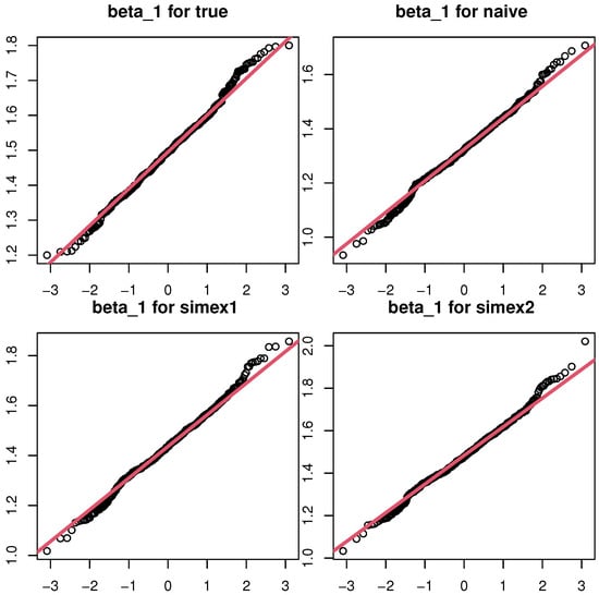
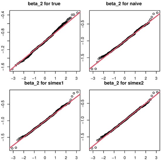
Figure 1. Q-Q plots of various estimators of ${\beta }_1=1.5$ (left panel) and ${\beta }_2=-1$ (right panel) in case 2 with sample size $n=100$.

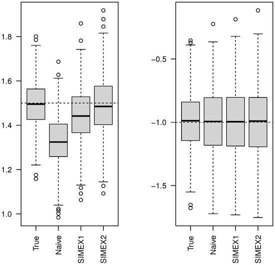
Figure 2. Boxplots of various estimators of ${\beta }_1=1.5$ (left panel) and ${\beta }_2=-1$ (right panel) in case 2 with sample size $n=100$.

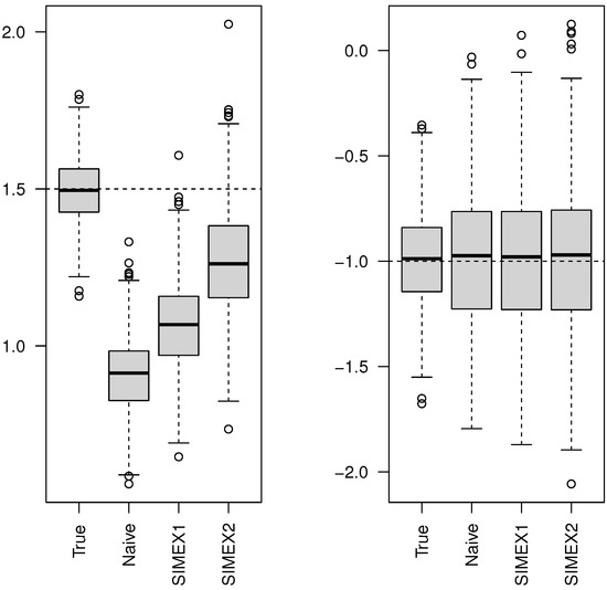
Figure 3. Boxplots of various estimators of ${\beta }_1=1.5$ (left panel) and ${\beta }_2=-1$ (right panel) in case 3 with sample size $n=100$.

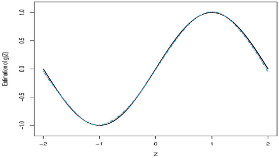
Figure 4. Average estimated curve of $g\left(z\right)=sin(\pi z/2)$ in case 2 with sample size $n=100$. The segment line (gray) is the true curve. The solid line (black), the dotted line (red), the dot–dashed lines (green and blue) correspond to the oracle estimator, naive estimator, SIMEX1 estimator, and SIMEX2 estimator, respectively.

4. Real Data Analysis

To illustrate the proposed procedure, an application regarding body fat data is provided. These data are available at http://lib.stat.cmu.edu/datasets/bodyfat (accessed on 1 January 2020) and have been analyzed by several authors in different contexts; see [8,10,24]. There are 252 observations and several variables, including the percentage of body fat as the response variable Y, and 13 explanatory variables: age ($X_1$), weight ($X_2$), height ($X_3$), neck ($X_4$), chest ($X_5$), abdomen ($X_6$), hip ($X_7$), thigh ($X_8$), knee ($X_9$), ankle ($X_{10}$), biceps ($X_{11}$), forearm ($X_{12}$), and wrist ($X_{13}$). As in [10], we deleted all possible outliers and obtained a sample size of 248. Following [8], we selected chest ($X_5$) as the nonlinear effect U, and the other 12 covariates were treated as the linear component X in Model (1). Motivated by the suggestion in [24], weight ($X_2$) was presumed to be mismeasured, and others were presumed to be error-free. Similar to [10], before the forthcoming computation, the nonparametric part U was transformed into [0,1] and the other covariates were standardized.

Estimation results of the regression coefficients $\beta$ using the naive method and SIMEX methods with linear or quadratic extrapolation functions are shown in Table 4 and Table 5, associated with the results presented in [8] (local linear LARE estimator) and [10] (local linear LPRE estimator), which are denoted by Naive, SIMEX1, SIMEX2, ZW, and CL, respectively. To evaluate the impact of the measurement error level ${\sigma }^2$ and the number of interior knots $k_n$, the variance in the measurement error and the number were set to 0.1 and 0.3, 3, and 6, respectively. This means that four cases were considered. In each specific case, the estimates of regression coefficients were close to each other. However, the estimates of the coefficient associated with weight ($X_2$) varied greatly. In particular, for the the coefficient of $X_2$, the sign of the naive estimate was negative, but the SIMEX estimates were both positive, although their absolute values were small. As the level of measurement error increased, the changes in SIMEX estimates varied steadily.

Table 4. Estimation results for the body fat data when $k_n=3$.

		${\mathit{\sigma }}^2=0.1$			${\mathit{\sigma }}^2=0.3$
	Naive	SIMEX1	SIMEX2		SIMEX1	SIMEX2		CL	ZW
Age	0.0677	0.0722	0.0729		0.0724	0.0731		0.0702	0.1476
Weight	−0.0719	0.0128	0.0138		0.0136	0.0141		−0.1346	−0.3945
Height	−0.0028	−0.0094	−0.0072		−0.0093	−0.0074		0.0066	0.1050
Neck	−0.0745	−0.0792	−0.0793		−0.0795	−0.0794		−0.0698	−0.066
Abdomen	0.5496	0.5352	0.5350		0.5333	0.5321		0.5432	0.8309
Hip	−0.0809	−0.1026	−0.1020		−0.1037	−0.1024		−0.0996	−0.1936
Thigh	0.0881	0.0817	0.0787		0.0824	0.0792		0.1257	0.1665
Knee	0.0004	−0.0007	0.0016		−0.0002	0.0020		−0.0013	−0.0259
Ankle	0.0061	0.0013	0.0027		0.0012	0.0029		0.0153	0.0407
Biceps	0.0195	0.0185	0.0200		0.0182	0.0199		0.0292	0.1103
forearm	0.0297	0.0258	0.0249		0.0255	0.0249		0.0377	0.0723
Wrist	−0.0944	−0.1011	−0.1047		−0.1014	−0.1047		−0.0838	−0.0860

Table 5. Estimation results for the body fat data when $k_n=3$.

		${\mathit{\sigma }}^2=0.1$			${\mathit{\sigma }}^2=0.3$
	Naive	SIMEX1	SIMEX2		SIMEX1	SIMEX2		CL	ZW
Age	0.0786	0.0733	0.0716		0.0731	0.0723		0.0702	0.1476
Weight	−0.2005	0.0110	0.0113		0.0113	0.0120		−0.1463	−0.3945
Height	0.0381	−0.0085	−0.0014		−0.0087	−0.0014		0.0066	0.1050
Neck	−0.0861	−0.0858	−0.0962		−0.0854	−0.0956		−0.0698	−0.066
Abdomen	0.5309	0.5309	0.5330		0.5317	0.5285		0.5432	0.8309
Hip	0.0254	−0.1039	−0.1098		−0.1033	−0.1077		−0.0996	−0.1936
Thigh	0.1036	0.0873	0.0881		0.0867	0.0860		0.1257	0.1665
Knee	−0.0346	−0.0010	0.0010		−0.0013	0.0024		−0.0013	−0.0259
Ankle	0.0168	−0.0019	−0.0108		−0.0019	−0.0106		0.0153	0.0407
Biceps	0.0193	0.0175	0.0129		0.0179	0.0127		0.0292	0.1103
Forearm	0.0161	0.0269	0.0373		0.0268	0.0374		0.0377	0.0723
Wrist	−0.0827	−0.1012	−0.1013		−0.1009	−0.1040		−0.0838	−0.086

The estimated curves of $g(.)$ are plotted in Figure 5 and Figure 6. All curves had a similar trend. In other words, $g\left(U\right)$ firstly increased until around $U=0.4$, and then it then decreased. This phenomenon was also found in [10], but their figures behaved less clearly than ours. For a fixed number of knots, the level of measurement error had little effect on the estimated curves. Instead, the difference between Figure 5 and Figure 6 was relatively large, which may have been caused by the overfitting when $k_n$ was 6 and underfiting when $k_n$ was 3. It is worth noting that the SIMEX estimates were less sensitive than the naive estimate in all cases.

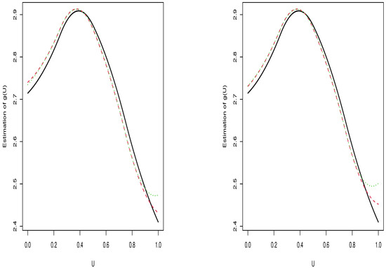
Figure 5. Estimated curves of $g\left(U\right)$ when $k_n=3$. The left (right) panel corresponds to the case with ${\sigma }^2=0.1$ (${\sigma }^2=0.3$). The solid line (black), the dotted line (red), and the dashed lines (green) correspond to the naive estimator, SIMEX1 estimator, and SIMEX2 estimator, respectively.

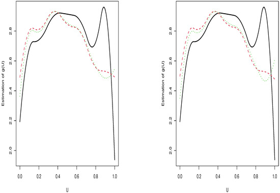
Figure 6. Estimated curves of $g\left(U\right)$ when $k_n=6$. The left (right) panel corresponds to the case with ${\sigma }^2=0.1$ (${\sigma }^2=0.3$). The solid line (black), the dotted line (red), and the dashed lines (green) correspond to the naive estimator, SIMEX1 estimator, and SIMEX2 estimator, respectively.

5. Conclusions

In this study, we used the simulation–extrapolation method to estimate the regression parameters and the nonparametric function in the partially linear multiplicative regression model in Models (1) and (2) based on the LPRE loss function and B-spline approximation, where covariates in the linear part are measured with additive measurement errors, but the nonparametric part is exactly observed. Under some regularity conditions, the SIMEX estimates were asymptotically normal with a more complex covariance matrix structure than naive estimates. Furthermore, extensive numerical studies show that our proposed method performs better than naive estimators when the measurement error is moderate or heavy, and it is comparable with the naive estimators when the measurement error is light. As the covariate in the nonparametric component is error-free, the resulting estimates of the nonparametric function are always well-fitted.

As indicated in Section 1, the approaches proposed in this paper may be adapted to the other more general models, such as the partially linear additive model as in [20], or single-index or varying-coefficient multiplicative regression models. Our future work will also consider extensions of them in fields with covariate measurement errors in all covariates, censored data, or longitudinal data analysis, which is meaningful for practitioners. As indicated by one referee, the model in Models (1) and (2) assumed that the measurement error only occurred in the linear part. In fact, the nonlinear part may be measured with error. For the later case, our method can still be implemented as in [20], except some minor modifications. However, the asymptotic theory becomes troublesome. Furthermore, as in [16], how to identify which set of covariates lies in the linear part or the nonlinear part is interesting. Additionally, when the dimension of covariates is high, how to effectively select the true important variables deserves to be studied thoroughly. All these issues will be investigated in the future.

References

- Chen, K.; Guo, S.; Lin, Y.; Ying, Z. Least absolute relative error estimation. J. Am. Stat. Assoc. 2010, 105, 1104–1112. [Google Scholar] [CrossRef] [PubMed]
- Khoshgoftaar, T.M.; Bhattacharyya, B.B.; Richardson, G.D. Predicting software errors, during development, using nonlinear regression models: A comparative study. IEEE Trans. Reliab. 1992, 41, 390–395. [Google Scholar] [CrossRef]
- Narula, S.C.; Wellington, J.F. Prediction, linear regression and the minimum sum of relative errors. Technometrics 1977, 19, 185–190. [Google Scholar] [CrossRef]
- Park, H.; Stefanski, L.A. Relative-error prediction. Statist. Probab. Lett. 1998, 40, 227–236. [Google Scholar] [CrossRef]
- Chen, W.; Wan, M. Penalized Spline Estimation for Nonparametric Multiplicative Regression Models. J. Appl. Stat. 2023. submitted. [Google Scholar]
- Chen, K.; Lin, Y.; Wang, Z.; Ying, Z. Least product relative error estimation. J. Multivar. Anal. 2016, 144, 91–98. [Google Scholar] [CrossRef]
- Hirose, K.; Masuda, H. Robust relative error estimation. Entropy 2018, 20, 632. [Google Scholar] [CrossRef]
- Zhang, Q.; Wang, Q. Local least absolute relative error estimating approach for partially linear multiplicative model. Stat. Sinica 2013, 23, 1091–1116. [Google Scholar] [CrossRef]
- Zhang, J.; Feng, Z.; Peng, H. Estimation and hypothesis test for partial linear multiplicative models. Comput. Stat. Data Anal. 2018, 128, 87–103. [Google Scholar] [CrossRef]
- Chen, Y.; Liu, H. A new relative error estimation for partially linear multiplicative model. Commun. Stat. Simul. Comput. 2021, 1–19. [Google Scholar] [CrossRef]
- Liu, H.; Xia, X. Estimation and empirical likelihood for single-index multiplicative models. J. Stat. Plan. Inference 2018, 193, 70–88. [Google Scholar] [CrossRef]
- Zhang, J.; Zhu, J.; Feng, Z. Estimation and hypothesis test for single-index multiplicative models. Test 2019, 28, 242–268. [Google Scholar] [CrossRef]
- Zhang, J.; Cui, X.; Peng, H. Estimation and hypothesis test for partial linear single-index multiplicative models. Ann. Inst. Stat. Math. 2020, 72, 699–740. [Google Scholar] [CrossRef]
- Hu, D.H. Local least product relative error estimation for varying coefficient multiplicative regression model. Acta Math. Appl. Sin. Engl. Ser. 2019, 35, 274–286. [Google Scholar] [CrossRef]
- Chen, Y.; Liu, H.; Ma, J. Local least product relative error estimation for single-index varying-coefficient multiplicative model with positive responses. J. Comput. Appl. Math. 2022, 415, 114478. [Google Scholar] [CrossRef]
- Ming, H.; Liu, H.; Yang, H. Least product relative error estimation for identification in multiplicative additive models. J. Comput. Appl. Math. 2022, 404, 113886. [Google Scholar] [CrossRef]
- Carroll, R.J.; Ruppert, D.; Stefanski, L.A.; Crainiceanu, C.M. Measurement Error in Nonlinear Models: A Modern Perspective, 2nd ed.; Chapman and Hall/CRC: New York, NY, USA, 2006. [Google Scholar]
- Tian, Y. Simulation-Extrapolation Estimation for Multiplicative Regression Model with Measurement Error. Master’s Thesis, Shanxi Normal University, Xi’an, China, 2020. [Google Scholar]
- Cook, J.R.; Stefanski, L.A. Simulation-extrapolation estimation in parametric measurement error models. J. Am. Stat. Assoc. 1994, 89, 1314–1328. [Google Scholar] [CrossRef]
- Liang, H.; Thurston, S.W.; Ruppert, D.; Apanasovich, T.; Hauser, R. Additive partial linear models with measurement errors. Biometrika 2008, 95, 667–678. [Google Scholar] [CrossRef]
- Chen, L.P.; Yi, G.Y. Analysis of noisy survival data with graphical proportional hazards measurement error models. Biometrics 2021, 77, 956–969. [Google Scholar] [CrossRef]
- Afzal, A.R.; Dong, C.; Lu, X. Estimation of partly linear additive hazards model with left-truncated and right-censored data. Stat. Model. 2017, 6, 423–448. [Google Scholar] [CrossRef]
- Chen, W.; Ren, F. Partially linear additive hazards regression for clustered and right censored data. Bull. Inform. Cybern. 2022, 54, 1–14. [Google Scholar] [CrossRef]
- Zhang, J.; Zhu, J.; Zhou, Y.; Cui, X.; Lu, T. Multiplicative regression models with distortion measurement errors. Stat. Pap. 2020, 61, 2031–2057. [Google Scholar] [CrossRef]
Disclaimer/Publisher’s Note: The statements, opinions and data contained in all publications are solely those of the individual author(s) and contributor(s) and not of MDPI and/or the editor(s). MDPI and/or the editor(s) disclaim responsibility for any injury to people or property resulting from any ideas, methods, instructions or products referred to in the content. |
© 2023 by the authors. Licensee MDPI, Basel, Switzerland. This article is an open access article distributed under the terms and conditions of the Creative Commons Attribution (CC BY) license (https://creativecommons.org/licenses/by/4.0/).