Generalized Finsler Geometry and the Anisotropic Tearing of Skin

Abstract

A continuum mechanical theory with foundations in generalized Finsler geometry describes the complex anisotropic behavior of skin. A fiber bundle approach, encompassing total spaces with assigned linear and nonlinear connections, geometrically characterizes evolving configurations of a deformable body with the microstructure. An internal state vector is introduced on each configuration, describing subscale physics. A generalized Finsler metric depends on the position and the state vector, where the latter dependence allows for both the direction (i.e., as in Finsler geometry) and magnitude. Equilibrium equations are derived using a variational method, extending concepts of finite-strain hyperelasticity coupled to phase-field mechanics to generalized Finsler space. For application to skin tearing, state vector components represent microscopic damage processes (e.g., fiber rearrangements and ruptures) in different directions with respect to intrinsic orientations (e.g., parallel or perpendicular to Langer’s lines). Nonlinear potentials, motivated from soft-tissue mechanics and phase-field fracture theories, are assigned with orthotropic material symmetry pertinent to properties of skin. Governing equations are derived for one- and two-dimensional base manifolds. Analytical solutions capture experimental force-stretch data, toughness, and observations on evolving microstructure, in a more geometrically and physically descriptive way than prior phenomenological models.

1. Introduction

Finsler geometry and its generalizations suggest the possibility of enriched descriptions of numerous phenomena in mathematical physics, albeit at the likely expense of greater complexity in the analysis and calculations compared to Riemannian geometry. Fundamentals of Finsler geometry, aptly credited to Finsler [1], are discussed in the classic monograph of Rund and the more recent text of Bao et al. [2,3]. See also the overview article by Eringen [4]. A monograph by Bejancu [5] and research cited therein [6,7,8] cover more generalized Finsler and pseudo-Finsler geometries, as do several more recent works [9,10].

Generalized Finsler geometry is predominantly used herein since strict classical Finsler geometry falls short in describing all phenomena pertinent to the present class of continuum behaviors. The broad physical sciences witness diverse implementations; a thorough recapitulation is outside the bounds of the current work. Available books discuss applications in optics, thermodynamics, and biology [11], as well as modern physical settings, including spinor-type structures [12]. Finsler geometry and its generalizations have also been used for describing anisotropic space-time, general relativity, quantum fields, gravitation, electromagnetism, and diffusion [13,14,15,16,17,18,19]. The current work implements a continuum mechanical framework for the physical response of solid bodies.

1.1. Background

Classical continuum mechanics, encompassing nonlinear elasticity and plasticity theories as example constitutive frameworks, is couched in the context of Riemannian–Cartan manifolds [20,21,22]. Non-vanishing torsion and/or curvature tensors may emerge, depending on linear connections introduced to describe various incompatibilities and possible sources of residual stresses, including dislocation and disclination in crystals [21,23,24,25], inhomogeneous temperature distributions [26,27], or biological growth [28,29,30].

In the classical Riemannian context, a continuous material body is treated as a manifold $\mathcal{M}$, differentiable and having dimension of n. Coordinate chart(s) $\left\{X^A\right\}$ ($A=1,\dots ,n$) provide parameterization. A Riemannian metric is introduced on $\mathcal{M}$; the components $G_{AB}=G_{AB}\left(X\right)$ comprise the metric tensor field. Dependency on components $X^A$ is implied by notational dependence on X [22]. The covariant derivative operator ∇, enabled by a linear connection on manifold $\mathcal{M}$, completes the geometric description. Associated linear connection coefficients generally consist of $n^3$ independent field components ${\Gamma }_{BC}^A={\Gamma }_{BC}^A\left(X\right)$. Although different dimensional spaces are admissible, $n=3$ is standard for the mechanics of solid continua. Bases of coordinates can be holonomic, or less commonly, anholonomic [31,32]. Anholonomic frames, for which continuous curves over $\mathcal{M}$ need not exist, arise when the deformation gradient is deconstructed in a multiplicative sense [33,34].

In the geometries of Finsler and various extensions, a differentiable $\mathcal{M}$, covered by chart(s) of coordinates $\left\{X^A\right\}$ ($A=1,\dots ,n$), is given. Denoted by $(\mathcal{Z},\mathcal{M},\Pi ,\mathcal{U})$ is a fiber bundle of the total space $\mathcal{Z}$, having a dimension of $n+m$. The slit tangent bundle $\mathcal{Z}\to T\mathcal{M}\setminus 0$ [3] is often associated with the total space with $m=n$, but such an association is not mandatory [5,9,10]. Auxiliary coordinates $\left\{D^K\right\}$ ($K=1,\dots ,m$) are assigned for every fiber $\mathcal{U}$. The total space $\mathcal{Z}$, therefore, has the parameter set $\{X^A,D^K\}$. Laws of transformation are derived for quantities depending on coordinates $(X,D)$, including holonomic bases. Coefficients of a nonlinear connection lead to bases that are non-holonomic. These bases advantageously change on $T\mathcal{M}$ in a standard manner for changes in base parameters $X^A$. To execute all possible forms of covariant differentiation—both horizontal and vertical—at least two and at most four sets of coefficients of linear connections are required, as outlined in [5,35].

The metric of the generalized pseudo-Finsler space has a functional dependency $G_{AB}=G_{AB}(X,D)$, which is always symmetric. In the classical geometry of Finsler, this metric is positive definite. In pseudo-Finsler geometry, positive definiteness is not essential [10]. The $G_{AB}$ are obtained as second partial derivatives of $\frac{1}{2}{\mathcal{F}}^2$ with respect to $D^A$ in strict Finsler geometry [2,3]. The fundamental Finsler function $\mathcal{F}$ is positively homogeneous of degree one with respect to D. As such, $G_{AB}$ is homogeneous of the zeroth degree with respect to D [2,3]. This implies that, for strict Finsler geometry, $G_{AB}$ shall not have dependence solely on the vector magnitude of an object consisting of the coordinates $\left\{D^A\right\}$. The existence of $\mathcal{F}$ and homogeneity of $G_{AB}$ are not required in more general kinds of Finsler spaces [5,6,18,36]. The functional dependence on $(X,D)$ for the metric and linear and nonlinear connection coefficients affects the derived quantities, such as curvature and torsion forms, as well as Stokes’ theorem [37].

The motivation for the geometry of Finsler in the mechanics of solid continua is as follows. Auxiliary coordinates $\left\{D^A\right\}$ are viewed as vectors at every material particle X. The concept generalizes micropolar, Cosserat, and broad kinds of micromorphic models [38,39,40,41,42,43] couched in Riemannian geometry to the extended Finsler geometry. In the usual theories, in contrast, the metric tensor is of the classical Riemannian form; coordinates $\left\{X^A\right\}$ are sufficient for functional dependencies. The director triads in micromorphic theories affect the governing equations and material response. However, these triads do not manifest in the metrics and connections in the same way as the D of the generalized Finsler space. Formulae for transformations of coordinates and the divergence theorem are simpler in the Riemannian versus the Finsler case.

1.2. Prior Work

The first application of Finsler geometry in the context of continuum mechanics of solids appears to be the treatment of ferromagnetic elastic–plastic crystals of Amari [44]. Conservation laws and field theories, with application to ferromagnetism, were further developed by Ikeda [45,46,47,48]. Bejancu [5] provided a generalized Finsler treatment of the kinematics of deformable bodies. More contemporary theories include those of Saczuk and Stumpf [49,50,51], with underpinnings in a monograph [52]. Different physical phenomena (e.g., different physical meanings of $\left\{D^K\right\}$ [51]) are encompassed by their models, which include kinematics, balance laws, and thermodynamics, but their focus is most often on the mechanics of elastic–plastic crystals and dislocations [49,50,52]. See also a recent theory presented in [53], which applies generalized Finsler geometry to topological defects, and the comprehensive review in [54] of prior works on generalized Finsler geometry in continuum physics.

A new theory of Finsler-geometric continuum mechanics was developed for nonlinear elastic solids with evolving microstructure, first published in the article [55] with a preliminary version in a technical report [56]. This variational theory was extended to allow for explicit inelastic deformation and applied to study phase transitions and shear localization in crystalline solids [55,57]. The theory has also been broadened for dynamics and shock waves [58,59], and most recently has been used to describe ferromagnetic solids [54], enriching the governing equations of Maugin and Eringen [60,61] with pertinent aspects arising from Finsler geometry [44,48].

Prior to this theory [54,55], pragmatic solutions to boundary value problems using continuum mechanical models incorporating generalized Finsler geometry appeared intractable due to the complexity of governing equations and unwieldy parameterizations (e.g., uncertain constitutive functions and material constants). Most aforementioned work [5,44,45,46,47,48,49,51,53] presented purely theoretical constructions without attempt to formulate or solve physical boundary value problems. A material response was calculated by Saczuk and Stumpf [50,52], but motion and internal state coordinates were prescribed a priori, without apparent solution of governing conservation laws for macroscopic and microscopic momentum and energy. In contrast, the present theory [55,56] appears to be the first Finsler geometry-based continuum mechanics theory for which analytical and numerical solutions to the governing equations have been found, as evidenced by solutions to numerous problems for (non)linear elastic materials with evolving microstructure (e.g., fractures, twinning, phase transitions, dislocations), as evidenced in those and subsequent works [54,55,56,57,58,59,62]. However, as discussed in Section 1.3, discrete models with a basis in Finsler geometry have successfully simulated the complex, nonlinear mechanical response of several real materials, including snakeskin [63].

All prior applications of the present theory [54,55] considered stiff crystalline solids or generic materials. The current research newly applies the theory to soft biological tissues, specifically the skin. Furthermore, prior applications in fracture and cavitation [54,55,59,62] were limited to either locally isotropic damage or to local material separation on a single cleavage plane. The current treatment advances the description of anisotropic fractures or ruptures on multiple material surfaces at a single point X. Most cited prior applications invoked only a single non-trivial state vector component in D (an exception being a multi-component D for twinning and fracture [59]) and most often conformal Weyl-type rescaling of $G_{AB}$ with canonically vanishing nonlinear connection (with a few exceptions studied, [57,62]). The current research incorporates an anisotropic generalized Finsler metric for multi-dimensional problems and non-trivial nonlinear connections to show utility by example.

1.3. Purpose and Scope

The scope of this paper covers two primary purposes:

• The demonstration of the utility of the generalized Finsler geometric theory for describing anisotropic elasticity and anisotropic structural rearrangements in soft biological tissue;
• The consolidation and refinement of the theory for the equilibrium (i.e., quasi-static) case.

The first item furnishes the first known application of Finsler geometry-based continuum theory to analyze finite-strain mechanics of soft biological tissue. Prior work of others [63,64] used ideas from Finsler geometry to model nonlinear stress–strain to failure responses of biological solids, but that work used a discrete, rather than continuum, theory with material points represented as vertices linked by bonds; interaction potentials comprised bonding energies within a Hamiltonian. In that promising and successful approach [65,66,67], a Finsler metric for bond stretch depends on the orientation of local microstructure entities (e.g., molecular chains or collagen fibers) described by the Finsler director vector field D. From a different modeling perspective, the current continuum theory considers, in a novel way, the effects of the microstructure on anisotropy (elastic and damage-induced) in both a geometric and constitutive sense. The second item includes a renewed examination of Rund’s divergence theorem [37] in the context of an osculating Riemannian metric. It is shown that certain choices of metric and connection coefficients, with the possible addition of a source term to the energy conservation law, can recover governing equations for biologic tissue growth [30] in the quasi-static limit (Appendix B).

1.3.1. Soft Tissue and Skin Mechanics

Most soft tissues have inherent directionality due to their collagen fiber-based and/or aligned cellular microstructures [68,69], toward which tools of analysis from Finsler geometry might be anticipated to aptly apply. The mechanics of skin deformation [68,70,71], degradation [72,73], and tearing [73,74] are investigated herein. Like most biological materials, the microstructure of skin is complex. The respective middle and outer layers of skin are the dermis and epidermis, with elastin, collagen fibers, and cells embedded in a ground matrix. The underlying hypodermis (i.e., adipose) can be labeled as an inner layer of the skin. The microstructure dictates nonlinear, anisotropic, viscoelastic, and tearing behaviors [74,75,76]. Mechanical behavior at small strains is primarily controlled by the elastin and ground substance, whereby collagen fibers are coiled or slack [75]. Under increasing tensile stretch, the collagen fibers straighten and tighten, supporting most of the load, and compliance decreases. Under more severe stretching, fibers slide, delaminate, and rupture, leading to reduced stiffness, strain softening, and material failure [72,73,74,77].

Experiments indicate that skin elasticity has orthotropic symmetry [68,70,71,75]. Orthotropy arises from preferred arrangements of the collagen fibers, leading to greater stiffness in the directions where more fibers are aligned. In the plane of the dermis, fibers tend to be dispersed about a primary axis along which stiffness is greatest. In vivo, resting skin tension is greatest along this axis, parallel to Langer’s lines [75]. In typical uniaxial and biaxial tests [68,70,71,74], extracted skin is unstretched initially, but the greater stiffness along the primary direction persists, with differences in stiffness also emerging between orthogonal in-plane and out-of-plane directions [70,75]. As might be expected, damage processes are also anisotropic due to fiber degradation that differs with respect to the direction of loading relative to the microstructure [73,74].

Skin, as is most biological tissue, is simultaneously nonlinear elastic, viscoelastic, and poroelastic [68,76,78,79]; the pertinence of mechanisms depends on the time scale of loading. The present application considers only monotonic loading at a constant rate (e.g., no cycling or rate fluctuations). Loading rates are assumed much slower or faster than viscous relaxation times. Thus, the pseudo-elastic approach is justified to study these experiments [68], whereby hyperelastic models are deemed reasonable [71,80,81,82,83], albeit noting that different elastic constants (e.g., static and dynamic moduli) are needed to fit data at vastly different limiting low and high loading rates [84,85]. In future applications to problems with time dependence, internal state variables can be extended, leading to kinetic laws with explicit viscous dissipation [78,86]. The current study is limited to relatively small samples, tested in vitro, under uniaxial or biaxial extension [68,70,74,87]. The material is modeled as unstressed initially and homogeneous with regard to elastic properties. In the future, the current theory can be extended to study residual stress due to growth or heterogeneous material features, as well as heterogeneous elastic properties. Residual stresses can be addressed, in the context of Riemannian manifolds, using a material metric having a non-vanishing Riemann–Christoffel curvature of its Levi–Civita connection [27,30] or an anholonomic multiplicative term in the deformation gradient [29,88]. These ideas may be extended to generalized Finsler space (e.g., invoking the current fiber bundle approach) in future.

An early nonlinear elastic model described orthotropic symmetry using a phenomenological pseudo-strain energy potential [89]. Another early model delineated the contributions of elastin and collagen fibers [79]. More recently, a class of nonlinear elastic models accounting for anisotropy from fiber arrangements using structure tensors has been successful in representing many soft tissues, including arterial walls [80,90], myocardium [82,91], and skin [71]. Polyconvex energy potentials can be incorporated for stability and to facilitate the existence of (unique) solutions to nonlinear elastic problems [81,90]. Fiber dispersion can be incorporated to modulate the degree of anisotropy [71,92]. To date, most damage models accounting for softening and failure have been phenomenological, whether implemented at the macroscopic scale (either isotropic or along preferred fiber directions) or the scale of individual fibers and their distributions [73,77,90,93]. These damage models, with a basis in continuum damage mechanics [94], are thermodynamically consistent in the sense that damage is dissipative, but their particular kinetic laws and (often numerous) parameters are calibrated to experimental data without much physical meaning. In contrast, the phase-field approach has been recently implemented for soft-tissue fracture or rupture, incorporating relatively few parameters with physical origin (e.g., surface energy) and regularization facilitating unique solutions to problems involving material softening [95,96]. The kinetic law or equilibrium equation for damage is derived from fundamental principles [97] and drives material to a local minimum-energy state, in contrast to ad hoc equations simply selected to match data.

1.3.2. Overview of the Current Work

Implementation of the present generalized Finsler theory consists of four key elements: definition of the internal state D, assignment of the metric tensor, assignment of the linear and nonlinear connections, and the prescription of the local free energy potential. For soft tissue mechanics, the state vector represents the fiber rearrangements. Damage anisotropy is monitored via its direction, with different components of D reflecting fiber reorganization and rupture with respect to orientations of the microstructure features [73,74]; the magnitude of each component of D measures the local intensity of damage in a given material direction. The metric tensor with components $G_{AB}(X,D)$ depends on position X as well as the direction and magnitude of D in the generalized Finsler space; novel D dependence encompasses the rescaling of the material manifold as damaged entities open, close, or rearrange in various directions [54,62]. The preferred linear connection is that of Chern and Rund [3], ensuring compatibility with the divergence theorem used to derive the Euler–Lagrange equations [54,55]. The generalized Finslerian D dependence of both the metric and linear connection explicitly affect the governing equations. Roles of nonlinear connections are newly examined; a non-trivial prescription is shown to influence the fracture energy and stress–strain response.

The free energy density consists of a nonlinear elastic contribution and an internal structure contribution. The nonlinear elastic potential enriches the orthotropic theory of Holzapfel, Ogden, Gasser, and others [71,80,82,83,92] with implicit contributions from the generalized Finsler metric as well as anisotropic degradation from D. The structural contribution is motivated by phase-field mechanics [95,98]. A previous model for arterial dissection [95] accounted for fiber-scale damage anisotropy using a scalar order parameter. The current theory invokes a more physically descriptive, vector-valued order parameter (i.e., normalized D) of the generalized Finsler type. With regard to skin experiments, solutions obtained for the current model are shown to admirably match extension and failure data, including stress–strain behavior and fracture toughness [73,74,99] with parameters having physical or geometric origins. The general theory is, thus, potentially more physically realistic, and considered more descriptive from a geometric perspective, than past models based on phenomenological damage mechanics [90,94,100,101].

This paper is organized as follows. Mathematical preliminaries (e.g., notation and definitions for objects in referential and spatial configurations) are provided in Section 2. The Finsler-geometric theory of continuum mechanics is presented in Section 3, including kinematics of finite deformation and equilibrium equations derived with a variational approach. The next two sections specialize the theory of modeling soft tissue, specifically skin. In Section 4, a one-dimensional (1D) model for the base manifold $\mathcal{M}$ is formulated. Analytical and semi-numerical solutions are obtained for uniaxial extension and compared to experimental data. In Section 5, a two-dimensional (2D) model for $\mathcal{M}$ is formulated, whereby the skin has orthotropic symmetry; solutions are obtained for biaxial extension with anisotropic damage in orthogonal material directions. The conclusions follow in Section 6.

2. Generalized Finsler Space

The content of Section 2 consolidates a more thorough exposition given in a recent review [54], from which notation is adopted. Other extensive texts include those of Rund, Bejancu, and Bao et al. [2,3,5]. A new contribution in the present Section 2 is an interpretation of the divergence theorem [37,54] using an osculating Riemannian metric, whereby for the further simplifying assumption of the vanishing nonlinear connection, a representation akin to that of classical Riemannian geometry is obtained.

2.1. Reference Configuration

The very general fiber bundle approach of Bejancu [5] encompasses geometric fundamentals of the theory. A reference configuration is linked to a specific time t, where the material body is viewed as undeformed, relative to some intrinsic state. The manifold, denoted by $\mathcal{M}$, is differentiable and of dimension n. One can classically immerse the true continuous body in the Euclidean N space with restriction $N\ge n$.

Remark 1. 

This kind of immersion exclusively holds only for the base space $\mathcal{M}$. As defined below, the fiber bundle’s total space $\mathcal{Z}$ does not usually obey, such an embedding [2,102,103]. Likewise, a Finsler space $F_n$ does not fulfill this type of Euclidean embedding.

A particle of the material occupies each point $X\in \mathcal{M}$. Notation $\left\{X^A\right\}(A=1,2,\dots ,n)$ defines a chart of material coordinates on $\mathcal{M}$. Coverage of $\mathcal{M}$ by any individual chart need not be complete. Let $\mathit{D}$ denote a vector field assigned to every particle. Accordingly, the $\left\{D^K\right\}(K=1,2,\dots ,m)$ are viewed as additional coordinates for $\mathcal{M}$. Parameters $\left\{D^K\right\}$ are, by construction, of sufficient smoothness: field $\mathit{D}$ is presumed differentiable over $\mathcal{M}$, of any necessary class, with respect to material coordinates $\left\{X^A\right\}$.

Let $\mathcal{Z}$ be the total space having dimension $n+m$. The fiber bundle is $\mathsf{Z}=(\mathcal{Z},\Pi ,\mathcal{M},\mathcal{U})$. The projection is $\Pi :\mathcal{Z}\to \mathcal{M}$. A fiber at point X is $\mathcal{U}={\mathcal{Z}}_X={\Pi }^{-1}\left(X\right)$. The dimension of a vector space represented by each fiber is n, where a vector bundle is $(\mathcal{Z},\Pi ,\mathcal{M})$. The set $\{X^A,D^K\}$ serves as a (local) chart for (a portion of) $\mathcal{Z}$. Denote an open neighborhood about $X\in \mathcal{M}$ by ${\mathcal{M}}^{\prime }\subset \mathcal{M}$. Let $P_1$ be the projection operator to the first factor, and write an isomorphism for vector spaces as $\Phi$. Commutation follows for the diagram below [5]:

2.1.1. Coordinate Transformations

Transformations for charts of both sets of coordinates $\{X,D\}$ to $\{\tilde{X},\tilde{D}\}$ on total space $\mathcal{Z}$ are defined as [5,10]

$${\tilde{X}}^A={\tilde{X}}^A\left(X\right),{\tilde{D}}^J(X,D)=Q_K^J\left(X\right)D^K.$$

(1)

The transformation matrix $Q_K^J$ fulfills ${\tilde{Q}}_K^I{Q}_J^K={\delta }_J^I$, presumably differentiable and non-singular. As usual, ${\delta }_J^I=1\forall I=J,{\delta }_J^I=0\forall I\ne J$. Let $T\mathcal{Z}$ denote the tangent bundle, and $\{\frac{\partial }{\partial X^A},\frac{\partial }{\partial D^K}\}$ denote the holonomic frame field or holonomic basis. Let $T^{*}\mathcal{Z}$ be the cotangent bundle and $\{d{X}^A,d{D}^K\}$ its holonomic coordinate basis. The transformation law for holonomic frames on $T\mathcal{Z}$, for coordinate changes $(X,D)\to (\tilde{X},\tilde{D})$ on $\mathcal{Z}$ per base coordinate changes $X\to \tilde{X}$ on manifold $\mathcal{M}$, consistent with (1) is [5,10]

$$\frac{\partial }{\partial {\tilde{X}}^A}=\frac{\partial X^B}{\partial {\tilde{X}}^A}\frac{\partial }{\partial X^B}+\frac{\partial D^K}{\partial {\tilde{X}}^A}\frac{\partial }{\partial D^K}=\frac{\partial X^B}{\partial {\tilde{X}}^A}\frac{\partial }{\partial X^B}+\frac{\partial {\tilde{Q}}_J^K}{\partial {\tilde{X}}^A}{\tilde{D}}^J\frac{\partial }{\partial D^K},$$

(2)

$$\frac{\partial }{\partial {\tilde{D}}^J}=\frac{\partial X^B}{\partial {\tilde{D}}^J}\frac{\partial }{\partial X^B}+\frac{\partial D^K}{\partial {\tilde{D}}^J}\frac{\partial }{\partial D^K}={\tilde{Q}}_J^K\frac{\partial }{\partial D^K}.$$

(3)

Likewise, on $T^{*}\mathcal{Z}$,

$$d{\tilde{X}}^A=\frac{\partial {\tilde{X}}^A}{\partial X^B}d{X}^B+\frac{\partial {\tilde{X}}^A}{\partial D^K}d{D}^K=\frac{\partial {\tilde{X}}^A}{\partial X^B}d{X}^B,$$

(4)

$$d{\tilde{D}}^J=\frac{\partial {\tilde{D}}^J}{\partial X^B}d{X}^B+\frac{\partial {\tilde{D}}^J}{\partial D^K}d{D}^K=\frac{\partial Q_K^J}{\partial X^B}{D}^{K}d{X}^B+Q_K^{J}d{D}^K.$$

(5)

Given (1), $\left\{\frac{\partial }{\partial X^A}\right\}$ and $\left\{d{D}^K\right\}$ map differently than standard vectorial objects on $\mathcal{Z}$. Define [5,9]

$$\frac{\delta }{\delta X^A}=\frac{\partial }{\partial X^A}-N_A^K\frac{\partial }{\partial D^K},\delta D^K=d{D}^K+N_B^{K}d{X}^B.$$

(6)

Non-holonomic basis vectors $\left\{\frac{\delta }{\delta X^A}\right\}$ and $\left\{\delta D^K\right\}$ obey [10]

$$\frac{\delta }{\delta {\tilde{X}}^A}=\frac{\partial X^B}{\partial {\tilde{X}}^A}\frac{\delta }{\delta X^B},\delta {\tilde{D}}^J=Q_K^J\delta D^K;⟨\frac{\delta }{\delta X^B},d{X}^A⟩={\delta }_B^A,⟨\frac{\partial }{\partial D^K},\delta D^J⟩={\delta }_K^J.$$

(7)

The set $\{\frac{\delta }{\delta X^A},\frac{\partial }{\partial D^K}\}$ is implemented over $T\mathcal{Z}$ for a local basis; likewise, on $T^{*}\mathcal{Z}$, a dual basis is taken to be $\{d{X}^A,\delta D^K\}$ [3,9]. The $N_B^K(X,D)$ are the coefficients of the nonlinear connection, serving as differentiable functions of their arguments. For (7) to hold under coordinate changes $X\to \tilde{X}$ [3,5],

$${\tilde{N}}_A^J=\left(Q_K^J{N}_B^K-\frac{\partial Q_K^J}{\partial X^B}{D}^K\right)\frac{\partial X^B}{\partial {\tilde{X}}^A},$$

(8)

meaning that nonlinear connections do not follow the transformation laws of linear connections. Nonlinear coefficients do not instill covariant differentiation identical to linear coefficients.

Remark 2. 

The orthogonal decomposition afforded by $T\mathcal{Z}$ with the corresponding nonlinear connection is $T\mathcal{Z}=V\mathcal{Z}\oplus H\mathcal{Z}$. The vertical vector bundle is $V\mathcal{Z}$ with $\left\{\frac{\partial }{\partial D^A}\right\}$ being its local frame field, and the horizontal distribution is $H\mathcal{Z}$ with the local field of frames $\left\{\frac{\delta }{\delta X^A}\right\}$ [5].

Respective fiber dimensions of $V\mathcal{Z}$ and $H\mathcal{Z}$ are m and n, and are possibly different. For the remainder of this work, let $m=n$, so that the horizontal and vertical spaces have identical dimensionality. Regarding notation, coordinate indices such as $J,K,\dots$ are interchangeable with $A,B,\dots$ for Einstein’s sums, now spanning 1 to n. Furthermore, for (1), consider

$$Q_B^A=\frac{\partial {\tilde{D}}^A}{\partial D^B}=\frac{\partial {\tilde{X}}^A}{\partial X^B}.$$

(9)

Relation (9) is obtained via soldering forms by Minguzzi [10]. Coordinate differentiation operations are expressed as follows, with f being a differentiable function of arguments $(X,D)$:

$${\partial }_{A}f(X,D)=\frac{\partial f(X,D)}{\partial X^A},{\overline{\partial }}_{A}f(X,D)=\frac{\partial f(X,D)}{\partial D^A};{\delta }_A(·)=\frac{\delta (·)}{\delta X^A}={\partial }_A(·)-N_A^B{\overline{\partial }}_B(·).$$

(10)

Special cases $f\to X$ and $f\to D$ are written [54,55]

$${\partial }_B{X}^A=\frac{\partial X^A}{\partial X^B}={\delta }_B^A,{\overline{\partial }}_B{X}^A=0;{\partial }_B{D}^A=\frac{\partial D^A}{\partial X^B},{\overline{\partial }}_B{D}^A={\delta }_B^A.$$

(11)

2.1.2. Length, Area, and Volume

The Sasaki metric tensor [3,35,104] on $\mathcal{Z}$ supplies vectorial scalar products:

$$\mathcal{G}(X,D)=\mathit{G}(X,D)+\check{\mathit{G}}(X,D)=G_{AB}(X,D)d{X}^A\otimes d{X}^B+{\check{G}}_{AB}(X,D)\delta D^A\otimes \delta D^B;$$

(12)

$${\mathcal{G}}_{AB}=G_{AB}=\mathit{G}\left(\frac{\delta }{\delta X^A},\frac{\delta }{\delta X^B}\right)={\check{G}}_{AB}=\check{\mathit{G}}\left(\frac{\partial }{\partial D^A},\frac{\partial }{\partial D^B}\right)={\check{G}}_{BA}=G_{BA}={\mathcal{G}}_{BA}.$$

(13)

Regarding notation, $\mathit{G}$ and $\check{\mathit{G}}$ have equivalent components, hereafter written as $G_{AB}$, but subspaces spanned by these two tensors are orthogonal. Components in covariant form $G_{AB}$ and their inverse in contravariant form $G^{AB}$ enable respective lowering and raising of indices; G is the determinant of the $n\times n$ non-singular matrices of components of $\mathit{G}$ or $\check{\mathit{G}}$:

$$G^{AB}{G}_{BC}={\delta }_C^A;G(X,D)=det\left[G_{AB}(X,D)\right]=det\left[{\check{G}}_{AB}(X,D)\right].$$

(14)

Remark 3. 

Let $\mathit{V}=V^A\frac{\delta }{\delta X^A}\in H\mathcal{Z}$ denote a generic vector field on $\mathcal{Z}$. Then the magnitude of $\mathit{V}(X,D)$ is $|\mathit{V}|={⟨\mathit{V},\mathcal{G}\mathit{V}⟩}^{1/2}={⟨\mathit{V},\mathit{G}\mathit{V}⟩}^{1/2}={|\mathit{V}·\mathit{V}|}^{1/2}=|V^A{G}_{AB}{V}^B{|}^{1/2}={|V^A{V}_A|}^{1/2}\ge 0$, where $V^A$ and $G_{AB}$ are evaluated at $(X,D)$.

• When interpreted as a block diagonal $2n\times 2n$ matrix, the determinant of $\mathcal{G}$ is [49,50,52]

$$\mathcal{G}(X,D)=det\left[G_{AB}(X,D)\right]det\left[{\check{G}}_{AB}(X,D)\right]=|det\left[G_{AB}(X,D)\right]{|}^2={|G(X,D)|}^2.$$

(15)

Let $\mathrm{d}\mathit{X}$ be a local line element for the base manifold $\mathcal{M}$, referred to as the basis of $\left\{\frac{\delta }{\delta X^A}\right\}$, and let $\mathrm{d}\mathit{D}$ be a corresponding line element for the fiber $\mathcal{U}$, referred to as $\left\{\frac{\partial }{\partial D^A}\right\}$. Their lengths are, squared,

$${|\mathrm{d}\mathit{X}|}^2=⟨\mathrm{d}\mathit{X},\mathcal{G}\mathrm{d}\mathit{X}⟩=G_{AB}\mathrm{d}{X}^A\mathrm{d}{X}^B,{|\mathrm{d}\mathit{D}|}^2=⟨\mathrm{d}\mathit{D},\mathcal{G}\mathrm{d}\mathit{D}⟩=G_{AB}\mathrm{d}{D}^A\mathrm{d}{D}^B.$$

(16)

The respective volume element $\mathrm{d}V$ of $\mathcal{M}$, volume form $d\Omega$ of $\mathcal{M}$, and the area form $\Omega$ for its boundary $\partial \mathcal{M}$, are defined as follows [37], where $n=dim\mathcal{M}=dim\partial \mathcal{M}+1$:

$$\mathrm{d}V=\sqrt{G}\mathrm{d}{X}^1\mathrm{d}{X}^2\dots \mathrm{d}{X}^n,d\Omega =\sqrt{G}d{X}^1\wedge d{X}^2\wedge \dots \wedge d{X}^n,$$

(17)

$$\Omega =\sqrt{B}d{U}^1\wedge \dots \wedge d{U}^{n-1}.$$

(18)

Local coordinates on the hypersurface $\partial \mathcal{M}$, oriented and $(n-1)$-dimensional, are given as parametric equations $X^A=X^A\left(U^{\alpha }\right)(\alpha =1,\dots ,n-1)$, $B_{\alpha }^A=\frac{\partial X^A}{\partial U^{\alpha }}$, and $B=det\left(B_{\alpha }^A{G}_{AB}{B}_{\beta }^B\right)$.

2.1.3. Covariant Derivatives

Basis vector gradients in horizontal form are acquired from affine (i.e., linear) connection coefficients, written generically as $H_{BC}^A$ and $K_{BC}^A$, where $\nabla (·)$ is the covariant derivative:

$${\nabla }_{\delta /\delta X^B}\frac{\delta }{\delta X^C}=H_{BC}^A\frac{\delta }{\delta X^A},{\nabla }_{\delta /\delta X^B}\frac{\partial }{\partial D^C}=K_{BC}^A\frac{\partial }{\partial D^A}.$$

(19)

Analogously, vertical gradients employ generic connection coefficients, $V_{BC}^A$ and $Y_{BC}^A$:

$${\nabla }_{\partial /\partial D^B}\frac{\partial }{\partial D^C}=V_{BC}^A\frac{\partial }{\partial D^A},{\nabla }_{\partial /\partial D^B}\frac{\delta }{\delta X^C}=Y_{BC}^A\frac{\delta }{\delta X^A}.$$

(20)

For example, let $\mathit{V}=V^A\frac{\delta }{\delta X^A}\in H\mathcal{Z}$ be a vector field. Then the (total) covariant derivative of $\mathit{V}$ is

$$\begin{array}{cc}\hfill \nabla \mathit{V}& ={\nabla }_{\delta /\delta X^B}\mathit{V}\otimes d{X}^B+{\nabla }_{\partial /\partial D^B}\mathit{V}\otimes \delta D^B\hfill \\ & =({\delta }_B{V}^A+H_{BC}^A{V}^C)\frac{\delta }{\delta X^A}\otimes d{X}^B+({\overline{\partial }}_B{V}^A+Y_{BC}^A{V}^C)\frac{\partial }{\partial D^A}\otimes \delta D^B\hfill \\ & =V_{|B}^A\frac{\delta }{\delta X^A}\otimes d{X}^B+V^A{|}_B\frac{\partial }{\partial D^A}\otimes \delta D^B.\hfill \end{array}$$

(21)

Denoted by ${(·)}_{|A}$ is a horizontal covariant derivative with respect to $\left\{X^A\right\}$. Denoted by ${(·)|}_B$ is a vertical covariant derivative with respect to $\left\{D^B\right\}$.

Remark 4. 

The ordering of lower indices on connections matches some works [4,22,31,98] and is the transpose of others [2,5,34]. For symmetric connections, it is inconsequential.

The horizontal covariant derivative, in components of the horizontal metric tensor $\mathit{G}=G_{AB}d{X}^A\otimes d{X}^B$ (i.e., the horizontal part of $\mathcal{G}$), is

$$\begin{array}{cc}\hfill G_{AB|C}& ={\delta }_C{G}_{AB}-H_{CA}^D{G}_{DB}-H_{CB}^D{G}_{AD}\hfill \\ & ={\partial }_C{G}_{AB}-N_C^D{\overline{\partial }}_D{G}_{AB}-H_{CA}^D{G}_{DB}-H_{CB}^D{G}_{DA}.\hfill \end{array}$$

(22)

For the determinant of the metric $G=det\left(G_{AB}\right)$, identified as a scalar density [37],

$${\left(\sqrt{G}\right)}_{|A}={\partial }_A\left(\sqrt{G}\right)-N_A^B{\overline{\partial }}_B\left(\sqrt{G}\right)-\sqrt{G}{H}_{AB}^B.$$

(23)

The Levi–Civita connection coefficients are written as ${\gamma }_{BC}^A$; these are also known as Christoffel symbols of the second kind. Cartan’s tensor is $C_{BC}^A$, and horizontal coefficients of the Chern–Rund and Cartan connections are ${\Gamma }_{BC}^A$. All have null torsion due to symmetry:

$${\gamma }_{BC}^A=\frac{1}{2}{G}^{AD}({\partial }_C{G}_{BD}+{\partial }_B{G}_{CD}-{\partial }_D{G}_{BC})=G^{AD}{\gamma }_{BCD},$$

(24)

$$C_{BC}^A=\frac{1}{2}{G}^{AD}({\overline{\partial }}_C{G}_{BD}+{\overline{\partial }}_B{G}_{CD}-{\overline{\partial }}_D{G}_{BC})=G^{AD}{C}_{BCD},$$

(25)

$${\Gamma }_{BC}^A=\frac{1}{2}{G}^{AD}({\delta }_C{G}_{BD}+{\delta }_B{G}_{CD}-{\delta }_D{G}_{BC})=G^{AD}{\Gamma }_{BCD}.$$

(26)

Remark 5. 

The coefficients of Cartan, Chern, and Rund are compatible with regard to the covariant differential of $\mathit{G}=G_{AB}d{X}^A\otimes d{X}^B$ since $H_{BC}^A={\Gamma }_{BC}^A\Rightarrow G_{AB|C}=0$ for (22). Similarly, the tensor of Cartan is compatible with the vertical covariant differential of the metric $\mathit{G}$: $Y_{BC}^A=C_{BC}^A\Rightarrow G_{AB}{|}_C=0$.

From direct calculations with respective (24), (25), and (26), traces of linear connections are related to partial gradients of $G=det\left(\mathit{G}\right)$:

$${\partial }_A(ln\sqrt{G})={\gamma }_{AB}^B,{\overline{\partial }}_A(ln\sqrt{G})=C_{AB}^B,{\delta }_A(ln\sqrt{G})=\frac{1}{2}{G}^{BC}{\delta }_A{G}_{CB}={\Gamma }_{AB}^B.$$

(27)

Remark 6. 

Similar to the previous remark, $H_{BC}^A={\Gamma }_{BC}^A\Rightarrow G_{|A}=2G{(ln\sqrt{G})}_{|A}=0$ and $Y_{BC}^A=C_{BC}^A\Rightarrow G{{|}_A=2G(ln\sqrt{G})|}_A=0$.

Nonlinear connection coefficients $N_B^A(X,D)$ admissible under (1) and (8) can be obtained in various settings. If $T\mathcal{Z}$ is limited to sections that are locally flat [3,10], $N_B^A=0$ in a preferred coordinate chart $\{X,D\}$, but ${\tilde{N}}_B^A$ in (8) does not vanish for heterogeneous transformations under which ${\partial }_B{Q}_K^J$ is nonzero. A Lagrangian $\mathsf{L}(X,D)$, real and differentiable, can be introduced, from which $N_B^A={\mathsf{G}}_B^A$, where [5]

$${\mathsf{G}}_B^A={\overline{\partial }}_B{\mathsf{G}}^A={\overline{\partial }}_B\left[G^{AE}(D^C{\overline{\partial }}_E{\partial }_C\mathsf{L}-{\partial }_E\mathsf{L})\right].$$

(28)

Remark 7. 

Let $G_{AB}(X,D)$ be a positive homogeneous function of degree zero with respect to D. Then $G^A$ below are spray components [3,10], and $N_B^A=G_B^A$ are so-called canonical coefficients of the nonlinear connection that obey (8):

$$G^A=\frac{1}{2}{\gamma }_{BC}^A{D}^B{D}^C,G_B^A={\overline{\partial }}_B{G}^A.$$

(29)

For classification, let $K_{BC}^A=H_{BC}^A$ and $Y_{BC}^A=V_{BC}^A$. An extended and complete Finsler connection is written as the triplet $(N_B^A,H_{BC}^A,V_{BC}^A)$. The Chern–Rund connection is $(G_B^A,{\Gamma }_{BC}^A,0)$. Cartan’s connection is $(G_B^A,{\Gamma }_{BC}^A,C_{BC}^A)$. Berwald’s connection is $(G_B^A,G_{BC}^A,0)$, where $G_{BC}^A=N_{BC}^A={\overline{\partial }}_B{N}_C^A={\overline{\partial }}_B{\overline{\partial }}_C{G}^A$.

2.1.4. A Divergence Theorem

Let $\mathcal{M}$ denote a differentiable manifold with the dimension of n. Let $\partial \mathcal{M}$ be its $(n-1)$-dimensional boundary, a hypersurface positively oriented and of class $C^1$. The coordinate-free theorem of Stokes for any $C^1$ differentiable $(n-1)$ form $\mathit{\alpha }$ on $\mathcal{M}$ can be written as

$${\int }_{\mathcal{M}}d\mathit{\alpha }={\int }_{\partial \mathcal{M}}\mathit{\alpha }.$$

(30)

Theorem 1. 

Let $\mathcal{M}$, $dim\mathcal{M}=n$, as the base space for a generalized Finsler bundle of the total space $\mathcal{Z}$. The boundary $\partial \mathcal{M}$ is of positive orientation and class $C^1$, having $dim\partial \mathcal{M}=n-1$. Let $\mathit{\alpha }(X,D)=V^A(X,D)N_A(X,D)\Omega (X,D)$ denote a differentiable $(n-1)$ form. Let $\mathit{V}=V^A\frac{\delta }{\delta X^A}\in H\mathcal{Z}$ denote a vector field, and $V^A$ denote its contravariant components. Denote the positive-definite field $G_{AB}(X,D)$ as components of the metric on the horizontal space having $G=det\left(G_{AB}\right)>0$. Let $H_{BC}^A=H_{CB}^A$ be the symmetric and affine horizontal connection such that ${\left(\sqrt{G}\right)}_{|A}=0$. Lastly, $C^1$ functional relations $D=D\left(X\right)$ are presumed available for vertical coordinates of fibers for all $X\in \mathcal{M}$. Stokes’ theorem (30) can then be expressed explicitly as follows for an assigned chart $\left\{X^A\right\}$, appealing to definitions of forms for volumes and areas in the second of (17) and (18):

$${\int }_{\mathcal{M}}[V_{|A}^A+(V^A{C}_{BC}^C+{\overline{\partial }}_B{V}^A)D_{;A}^B]d\Omega ={\int }_{\partial \mathcal{M}}{V}^A{N}_A\Omega .$$

(31)

The horizontal covariant derivative is $V_{|A}^A={\delta }_A{V}^A+H_{BA}^B{V}^A$, the definition $D_{;A}^B={\partial }_A{D}^B+N_A^B$ with ${\partial }_A{D}^B=\partial D^A/\partial X^B$, and $N_A$ is a unit outward normal component of $\mathit{N}=N_{A}d{X}^A$ to $\partial \mathcal{M}$.

Proof. 

The proof, not repeated here, is given in the review [54], suggested but not derived formally in an earlier work [55]. The proof of (31) [54] extends that of Rund [37], which considered a strict Finsler space $F_n$ with the metric obtained from a fundamental function $\mathcal{F}$ and used Cartan’s connection $(G_B^A,{\Gamma }_{BC}^A,C_{BC}^A)$. The proof in [54] extends Rund’s proof to general Finsler spaces having arbitrary positive-definite $G_{AB}(X,D)$ and arbitrary $N_B^A(X,D)$.$\square$

Remark 8. 

As per the theorem of Stokes, (31) applies if the base space $\mathcal{M}$ and boundary $\partial \mathcal{M}$ is interchanged with a compact region of ${\mathcal{M}}^{\prime }\subset \mathcal{M}$ and its boundary of positive orientation.

Remark 9. 

The affine horizontal coefficients $H_{BC}^A={\Gamma }_{BC}^A$ of Cartan, Chern, and Rund uniquely fulfill symmetry and metric-compatibility requirements.

Remark 10. 

An alternative basis and the dual of that basis on $\mathcal{M}$ could be prescribed for the vector field $\mathit{V}$ and normal field $\mathit{N}$, given certain stipulations [54]. However, geometric interpretation of covariant differentiation on the left side of (31) suggests $\left\{\frac{\delta }{\delta X^A}\right\}$ should be used for $\mathit{V}$, by which, the dual basis $\left\{d{X}^B\right\}$ should be used for $\mathit{N}$ to ensure invariance: $⟨\mathit{V},\mathit{N}⟩\to V^A{N}_B⟨\frac{\delta }{\delta X^A},d{X}^B⟩$. If instead $\mathit{V}$ is referred to the holonomic basis $\left\{\frac{\partial }{\partial X^A}\right\}$, then $N_B^A=0$ should be imposed for invariance with $N_{B}d{X}^B$. As noted prior to (28), this choice would restrict (31) to homogeneous transformations of coordinates $\{X,D\}$.

As assumed in Theorem 1 [37,54,55], $C^1$ functions $D=D\left(X\right)$ must exist over all $X\in \mathcal{M}$. Relations of generalized Finsler geometry [5] still apply, but additional relations emerge naturally when metric $G_{AB}$ is interpreted as an osculating Riemannian metric [2,44]. Specifically, an alternative representation of (31) is newly proven in the following.

Corollary 1. 

Given $C^1$ functions $D=D\left(X\right)$, set ${\tilde{G}}_{AB}\left(X\right)=G_{AB}(X,D\left(X\right))$ as components of the osculating Riemannian metric derived from $\mathit{G}=G_{AB}d{X}^A\otimes d{X}^B$. Then (31) is equivalent to

$${\int }_{\mathcal{M}}{\tilde{V}}_{:A}^{A}d\Omega ={\int }_{\partial \mathcal{M}}{\tilde{V}}^A{\tilde{N}}_A\Omega ,$$

(32)

where the vector ${\tilde{V}}^A\left(X\right)=V^A(X,D\left(X\right))$, unit normal ${\tilde{N}}_A\left(X\right)=N_A(X,D\left(X\right))$, and covariant derivative ${\tilde{V}}_{:A}^A={\partial }_A{\tilde{V}}^A+{\tilde{\gamma }}_{BA}^B{\tilde{V}}^A$ with connection ${\tilde{\gamma }}_{BA}^B\left(X\right)={\partial }_A(ln\sqrt{\tilde{G}\left(X\right)})={\tilde{\gamma }}_{AB}^B\left(X\right)$ and $\tilde{G}=det\left({\tilde{G}}_{AB}\right)$.

Proof. 

The right of (32) is identical to the right of (31), given the change of variables. On the left of (32), from chain-rule differentiation, vanishing (23), and (27),

$${\partial }_A{\tilde{V}}^A={\partial }_A{V}^A+{\overline{\partial }}_B{V}^A{\partial }_A{D}^B,$$

(33)

$$\begin{array}{cc}\hfill {\tilde{V}}^A{\tilde{\gamma }}_{BA}^B& ={\tilde{V}}^A{\partial }_A(ln\sqrt{\tilde{G}})=V^A[{\partial }_A(ln\sqrt{G})+{\overline{\partial }}_B(ln\sqrt{G}){\partial }_A{D}^B]\hfill \\ & =V^A[{\delta }_A(ln\sqrt{G})+N_A^B{\overline{\partial }}_B(ln\sqrt{G})+C_{BC}^C{\partial }_A{D}^B]\hfill \\ & =V^A[{\delta }_A(ln\sqrt{G})+C_{BC}^C(N_A^B+{\partial }_A{D}^B)]\hfill \\ & =V^A[H_{AB}^B+C_{BC}^C{D}_{;A}^B]=V^A[H_{BA}^B+C_{BC}^C{D}_{;A}^B].\hfill \end{array}$$

(34)

Adding (33) to (34), and canceling $\pm N_A^B{\overline{\partial }}_B{V}^A$ terms, produces

$$\begin{array}{cc}\hfill {\tilde{V}}_{:A}^A& =\{{\partial }_A{V}^A+{\overline{\partial }}_B{V}^A{\partial }_A{D}^B-N_A^B{\overline{\partial }}_B{V}^A\}+\{N_A^B{\overline{\partial }}_B{V}^A+V^A[H_{BA}^B+C_{BC}^C{D}_{;A}^B]\}\hfill \\ \hfill & ={\delta }_A{V}^A+V^A{H}_{BA}^B+{\overline{\partial }}_B{V}^A({\partial }_A{D}^B+N_A^B)+V^A{C}_{BC}^C{D}_{;A}^B\hfill \\ & =V_{|A}^A+({\overline{\partial }}_B{V}^A+V^A{C}_{BC}^C)D_{;A}^B.\hfill \end{array}$$

(35)

Integrands on the left sides of (31) and (32) are, thus, verified to match, completing the proof.$\square$

Remark 11. 

Coefficients of the Levi–Civita connection of ${\tilde{G}}_{AB}$ satisfy the symmetry and metric-compatibility requirements used to prove (32):

$${\tilde{\gamma }}_{BC}^A=\frac{1}{2}{\tilde{G}}^{AD}({\partial }_C{\tilde{G}}_{BD}+{\partial }_B{\tilde{G}}_{CD}-{\partial }_D{\tilde{G}}_{BC})={\tilde{G}}^{AD}{\tilde{\gamma }}_{BCD}.$$

(36)

Remark 12. 

Given (36), the form of the divergence theorem in (32) appears analogous to that of a Riemannian manifold with boundary. It is not identical, however, since the non-holonomic basis $\left\{\frac{\delta }{\delta X^A}\right\}$ is used for $\mathit{V}$. As in Remark 2.1.3, the holonomic basis $\left\{\frac{\partial }{\partial X^A}\right\}$ could be used in a preferred chart $\{X,D(X\left)\right\}$, wherein $N_B^A=0$; under such special conditions the distinction vanishes.

2.1.5. Finsler and Pseudo-Finsler Spaces

The preceding presentation holds for generalized Finsler geometry, by which a Lagrangian function is not necessary to obtain components of the metric tensor [5,6,36]. Subclasses of generalized spaces of Finsler necessitate the existence of a Lagrangian $\mathcal{L}$. Denote the tangent bundle for $\mathcal{M}$ excluding the $D=0$ zero section as $\mathcal{Z}=T\mathcal{M}\setminus 0$. Function $\mathcal{L}(X,D):\mathcal{Z}\to \mathbb{R}$ is positively homogeneous of second order with respect to D and differentiable to any required class in $\left\{X^A\right\}$ and $\left\{D^A\right\}$, $C^{\infty }$ being the usual assumption [3], $C^5$ usually acceptable [10]. In this case, $(\mathcal{M},\mathcal{L})$ fulfills the requirements for a pseudo-Finsler space if $n\times n$ matrix $G_{AB}$ is both non-singular over $\mathcal{Z}$ and obtained from Lagrangian $\mathcal{L}$:

$$G_{AB}(X,D)={\overline{\partial }}_A{\overline{\partial }}_B\mathcal{L}(X,D),\mathcal{L}=\frac{1}{2}{G}_{AB}{D}^A{D}^B.$$

(37)

When $G_{AB}(X,D)$ is strictly positive definite on $\mathcal{Z}$, a pseudo-Finsler space becomes a Finsler space, written as the set $(\mathcal{M},\mathcal{F})$ or simply $F_n$ where $n=dim\mathcal{M}$. The fundamental function $\mathcal{F}(X,D)$ for the $F_n$ is first-order positively homogeneous with respect to D, whereby [2,3]

$$\begin{array}{cc}\hfill \mathcal{F}(X,D)=\sqrt{2\mathcal{L}(X,D)}& =|G_{AB}(X,D)D^A{D}^B{|}^{1/2}\hfill \\ & \leftrightarrow \mathcal{L}(X,D)=\frac{1}{2}{\mathcal{F}}^2(X,D);\mathcal{F}(X,D)>0\forall D\ne 0.\hfill \end{array}$$

(38)

In Finsler geometry [2,3,5], conditions $\mathsf{L}=\mathcal{L}$ and ${\mathsf{G}}^A=G^A$ in (28) and (29), and

$$\begin{array}{cc}\hfill G_{AB}& =\frac{1}{2}{\overline{\partial }}_A{\overline{\partial }}_B\left({\mathcal{F}}^2\right),G_B^A={\gamma }_{BC}^A{D}^C-C_{BC}^A{\gamma }_{DE}^C{D}^D{D}^E={\Gamma }_{BC}^A{D}^C;\hfill \\ \hfill C_{ABC}& =\frac{1}{4}{\overline{\partial }}_A{\overline{\partial }}_B{\overline{\partial }}_C\left({\mathcal{F}}^2\right).\hfill \end{array}$$

(39)

Reductions and embeddings for Finsler spaces are discussed elsewhere [2,3,10,54,102,103].

2.2. Spatial Configuration

A description of a fiber bundle analogous to that of Section 2.1 is invoked for the spatial or current representation of a continuum. Let $\mathfrak{m}$ and n denote the differentiable, spatial base manifold, and its dimension. Immersion in an external Euclidean N space is possible for the base manifold under stipulation $N\ge n$.

Remark 13. 

Definitions in Section 2.2 parallel those of Section 2.1. Upper-case symbols and indices for referential quantities are now exchanged with lower-case ones for most spatial variables.

In the current configuration, $x\in \mathfrak{m}$ depicts a point or particle location. A chart of spatial coordinates on $\mathfrak{m}$ is $\left\{x^a\right\}(a=1,2,\dots ,n)$. Every point on the spatial base manifold supports a local vector written as $\mathit{d}$, with $\left\{d^k\right\}(k=1,2,\dots ,m)$ auxiliary coordinates for $\mathfrak{m}$. The total space of dimension $n+m$ is $\mathfrak{z}$, and $\mathsf{z}=(\mathfrak{z},\pi ,\mathfrak{m},\mathfrak{u})$ is the fiber bundle. Let $\pi :\mathfrak{z}\to \mathfrak{m}$ be the projection. A fiber is $\mathfrak{u}={\mathfrak{z}}_x={\pi }^{-1}\left(x\right)$. Composite chart $\{x^a,d^k\}$ is associated with $\mathfrak{z}$. The vector bundle is ($\mathfrak{z},\pi ,\mathfrak{m})$; every fiber comprises a vector space of dimension n.

Denote the motion function by $\phi$, which globally maps reference material points to spatial points. Denote $\Xi =(\phi ,\theta )$ as the set of functions that correspondingly updates total spaces among configurations. General functional forms are $\phi (X,D):\mathcal{M}\to \mathfrak{m}$ and $\Xi (X,D):\mathcal{Z}\to \mathfrak{z}$. As described in Section 3.1, $\phi (X,D)$ and $\Xi (X,D)$ can have more specific representations [54]. Time (t) dependence is possible in the most general theories [50,58,59]. However, explicit time dependence is excluded from the current theoretical presentation that focuses on equilibrium configurations [55,62]. The following diagram commutes [5]:

2.2.1. Coordinate Transformations

Let $\{x,d\}$ to $\{\tilde{x},\tilde{d}\}$ be a change of coordinates for $\mathfrak{z}$; the Finsler relationships akin to (1) are

$${\tilde{x}}^a={\tilde{x}}^a\left(x\right),{\tilde{d}}^j(x,d)=q_k^j\left(x\right)d^k.$$

(40)

Differentiable matrix $q_k^j$ is non-singular with inverse ${\tilde{q}}_k^i$, whereby ${\tilde{q}}_k^i{q}_j^k={\delta }_j^i$. Tangent bundle $T\mathfrak{z}$ has $\{\frac{\partial }{\partial x^a},\frac{\partial }{\partial d^k}\}$ for its holonomic basis. The cotangent bundle $T^{*}\mathfrak{z}$ has $\{d{x}^a,d{d}^k\}$. Bases of non-holonomic vectors are $\left\{\frac{\delta }{\delta x^a}\right\}$ and $\left\{\delta d^k\right\}$; these map conventionally as $x\to \tilde{x}$:

$$\frac{\delta }{\delta x^a}=\frac{\partial }{\partial x^a}-N_a^k\frac{\partial }{\partial d^k},\delta d^k=d{d}^k+N_b^{k}d{x}^b.$$

(41)

The set $\{\frac{\delta }{\delta x^a},\frac{\partial }{\partial d^k}\}$ is used as a local basis on $T\mathfrak{z}$, and  $\{d{x}^a,\delta d^k\}$ is used for $T^{*}\mathfrak{z}$. The orthogonal decomposition of the tangent bundle, given its nonlinear connection, is $T\mathfrak{z}=V\mathfrak{z}\oplus H\mathfrak{z}$. Notation is as expected for the former vertical vector bundle and the latter horizontal distribution. Nonlinear connection coefficients transform as

$${\tilde{N}}_a^j=\left(q_k^j{N}_b^k-\frac{\partial q_k^j}{\partial x^b}{d}^k\right)\frac{\partial x^b}{\partial \widetilde{x^a}}.$$

(42)

Henceforth, set $m=n$. Thus, $j,k,\dots \to a,b,\dots$ for the index notation with sums covering 1 to n on repeated indices. Furthermore, per (40), the transformation for $d^a$ is akin to that of vectors of contravariant form on $\mathfrak{m}$:

$$q_b^a=\frac{\partial {\tilde{d}}^a}{\partial d^b}=\frac{\partial {\tilde{x}}^a}{\partial x^b}.$$

(43)

Condensed notation is used for derivatives with respect to coordinates on $\mathfrak{m},\mathfrak{z}$:

$${\partial }_{a}f(x,d)=\frac{\partial f(x,d)}{\partial x^a},{\overline{\partial }}_{a}f(x,d)=\frac{\partial f(x,d)}{\partial d^a};{\delta }_a(·)=\frac{\delta (·)}{\delta x^a}={\partial }_a(·)-N_a^b{\overline{\partial }}_b(·);$$

(44)

$${\partial }_b{x}^a=\frac{\partial x^a}{\partial x^b}={\delta }_b^a,{\overline{\partial }}_b{x}^a=0;{\partial }_b{d}^a=\frac{\partial d^a}{\partial x^b},{\overline{\partial }}_b{d}^a={\delta }_b^a.$$

(45)

2.2.2. Length, Area, and Volume

A scalar product for vectors on $\mathfrak{z}$ is obtained from the metric tensor of Sasaki [104]:

$$\mathfrak{g}(x,d)=\mathit{g}(x,d)+\check{\mathit{g}}(x,d)=g_{ab}(x,d)d{x}^a\otimes d{x}^b+{\check{g}}_{ab}(x,d)\delta d^a\otimes \delta d^b;$$

(46)

$${\mathfrak{g}}_{ab}=g_{ab}=\mathit{g}\left(\frac{\delta }{\delta x^a},\frac{\delta }{\delta x^b}\right)={\check{g}}_{ab}=\check{\mathit{g}}\left(\frac{\partial }{\partial d^a},\frac{\partial }{\partial d^b}\right)={\check{g}}_{ba}=g_{ba}={\mathfrak{g}}_{ba}.$$

(47)

Denote by $\mathrm{d}\mathit{x}$ and $\mathrm{d}\mathit{d}$, respectively, line elements of $\mathfrak{m}$ and $\mathfrak{u}$. The former has the basis vector $\left\{\frac{\delta }{\delta x^a}\right\}$, the latter $\left\{\frac{\partial }{\partial d^a}\right\}$. Line lengths squared satisfy

$${|\mathrm{d}\mathit{x}|}^2=⟨\mathrm{d}\mathit{x},\mathfrak{g}\mathrm{d}\mathit{x}⟩=g_{ab}\mathrm{d}{x}^a\mathrm{d}{x}^b,{|\mathrm{d}\mathit{d}|}^2=⟨\mathrm{d}\mathit{d},\mathfrak{g}\mathrm{d}\mathit{d}⟩=g_{ab}\mathrm{d}{d}^a\mathrm{d}{d}^b.$$

(48)

Let $dim\mathfrak{m}=n$ with $dim\partial \mathfrak{m}=n-1$ the dimension of the boundary. The local volume (scalar) element and volume form, followed by the local area form, are respectively

$$\mathrm{d}v=\sqrt{g}\mathrm{d}{x}^1\mathrm{d}{x}^2\dots \mathrm{d}{x}^n,d\omega =\sqrt{g}d{x}^1\wedge d{x}^2\wedge \dots \wedge d{x}^n,\omega =\sqrt{b}d{u}^1\wedge \dots \wedge d{u}^{n-1}.$$

(49)

The surface embedding in manifold $\mathfrak{m}$ is $x^a=x^a\left(u^{\alpha }\right)(\alpha =1,\dots ,n-1)$, $b_{\alpha }^a=\frac{\partial x^a}{\partial u^{\alpha }}$, and $b=det\left(b_{\alpha }^a{g}_{ab}{b}_{\beta }^b\right)$.

2.2.3. Covariant Derivatives

Let $\nabla (·)$ denote the operator for covariant differentiation. Generic affine coefficients $H_{bc}^a$ and $K_{bc}^a$ are used for horizontal derivatives, $V_{bc}^a$ and $Y_{bc}^a$ for vertical derivatives:

$${\nabla }_{\delta /\delta x^b}\frac{\delta }{\delta x^c}=H_{bc}^a\frac{\delta }{\delta x^a},{\nabla }_{\delta /\delta x^b}\frac{\partial }{\partial d^c}=K_{bc}^a\frac{\partial }{\partial d^a};$$

(50)

$${\nabla }_{\partial /\partial d^b}\frac{\partial }{\partial d^c}=V_{bc}^a\frac{\partial }{\partial d^a},{\nabla }_{\partial /\partial d^b}\frac{\delta }{\delta x^c}=Y_{bc}^a\frac{\delta }{\delta x^a}.$$

(51)

For example, on $\mathfrak{z}$ the covariant differential is obtained like (21), now for $\mathit{V}=V^a\frac{\delta }{\delta x^a}\in H\mathfrak{z}$:

$$\begin{array}{cc}\hfill \nabla \mathit{V}& ={\nabla }_{\delta /\delta x^b}\mathit{V}\otimes d{x}^b+{\nabla }_{\partial /\partial d^b}\mathit{V}\otimes \delta d^b=V_{|b}^a\frac{\delta }{\delta x^a}\otimes d{x}^b+V^a{|}_b\frac{\partial }{\partial d^a}\otimes \delta d^b.\hfill \end{array}$$

(52)

Herein, ${(·)}_{|a}$ and ${(·)|}_b$ denote differentiation horizontally with respect to $x^a$ and vertically with respect to $d^b$. Let ${\gamma }_{bc}^a$ be coefficients of the Levi–Civita connection on $\mathfrak{z}$, $C_{bc}^a$ be the coefficients of the Cartan tensor on $\mathfrak{z}$, and  ${\Gamma }_{bc}^a$ be the coefficients of Cartan, Chern, and Rund (horizontal) on $\mathfrak{z}$:

$${\gamma }_{bc}^a=\frac{1}{2}{g}^{ad}({\partial }_c{g}_{bd}+{\partial }_b{g}_{cd}-{\partial }_d{g}_{bc})=g^{ad}{\gamma }_{bcd},$$

(53)

$$C_{bc}^a=\frac{1}{2}{g}^{ad}({\overline{\partial }}_c{g}_{bd}+{\overline{\partial }}_b{g}_{cd}-{\overline{\partial }}_d{g}_{bc})=g^{ad}{C}_{bcd},$$

(54)

$${\Gamma }_{bc}^a=\frac{1}{2}{g}^{ad}({\delta }_c{g}_{bd}+{\delta }_b{g}_{cd}-{\delta }_d{g}_{bc})=g^{ad}{\Gamma }_{bcd}.$$

(55)

2.2.4. A Divergence Theorem

The generalized Finsler bundle of the total space $\mathfrak{z}$ is assigned base manifold $\mathfrak{m}$ noting $dim\mathfrak{m}=n$. The boundary denoted by $\partial \mathfrak{m}$ is of class $C^1$ and is of positive orientation. A vector field $\mathit{V}=V^a\frac{\delta }{\delta x^a}\in H\mathfrak{z}$ has contravariant components $V^a$. The $(n-1)$ form $\mathit{\alpha }(x,d)=V^a(x,d)n_a(x,d)\omega (x,d)$ is differentiable. Metric tensor components $g_{ab}(x,d)$, which are positive definite, apply for the horizontal distribution, and $g=det\left(g_{ab}\right)>0$. The affine horizontal connection $H_{bc}^a=H_{cb}^a$ is chosen to ensure ${\left(\sqrt{g}\right)}_{|a}=0$ (e.g., $H_{bc}^a={\Gamma }_{bc}^a$). The existence is required for fiber coordinates $d=d\left(x\right)$, representing functions of class $C^1$$\forall x\in \mathfrak{m}$. Forms for area and volume are defined in (49). Then (30) is in the coordinate form with respect to $\left\{x^a\right\}$,

$${\int }_{\mathfrak{m}}[V_{|a}^a+(V^a{C}_{bc}^c+{\overline{\partial }}_b{V}^a)d_{;a}^b]d\omega ={\int }_{\partial \mathfrak{m}}{V}^a{n}_a\omega .$$

(56)

Denoted by $n_a$ is the covector of the unit length normal to $\partial \mathfrak{m}$, $V_{|a}^a={\delta }_a{V}^a+V^a{H}_{ba}^b$, and $d_{;a}^b={\partial }_a{d}^b+N_a^b$. The proof matches that of Theorem 1 upon changes in variables; a corollary akin to Corollary1 also holds.

3. Finsler-Geometric Continuum Mechanics

The original theory of Finsler-geometric continuum mechanics [55,56] is formulated for finite strains with conservation of momenta applying at equilibrium states (i.e., quasi-static conditions). Subtle differences exist among certain assumptions for different instantiations, incrementally revised in successive works. Most differences are explained in a review [54].

3.1. Motion and Deformation

Let $\phi :\mathcal{M}\to \mathfrak{m}$ denote the motion of a material particle and $\Phi :\mathfrak{m}\to \mathcal{M}$ the inverse motion. These functions are differentiable of class $C^3$ and are one-to-one:

$$x^a={\phi }^a\left(X\right),X^A={\Phi }^A\left(x\right),(a,A=1,2,\dots ,n)$$

(57)

with $(\Phi \circ \phi )\left(X\right)=X$. Write $\Xi =(\phi ,\theta )$ to represent the motion in total, whereby $\Xi :\mathcal{Z}\to \mathfrak{z}$. Refer to Figure 1.

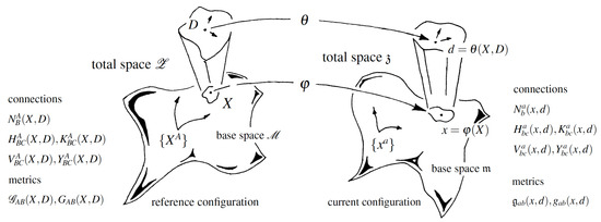
Figure 1. Total deformation $\Xi =(\phi ,\theta ):\mathcal{Z}\to \mathfrak{z}$ of material manifold $\mathcal{M}$ (dim $\mathcal{M}=n=m=2$) with base-space coordinates $\left\{X^A\right\}$ to spatial representation $\mathfrak{m}$ with base-space coordinates $\left\{x^a\right\}$. Internal structure fields are $(D,d)$ on total spaces $(\mathcal{Z},\mathfrak{z})$; arrows depict local components of state vectors $\mathit{D}$ and $\mathit{d}$ for neighborhoods centered at X and x.

Remark 14. 

The material field $\mathit{D}$ and spatial field $\mathit{d}$ are alternatively called director vectors or internal state vectors. They need not be unit vectors herein. The physical meanings of these fields depend on the particular application of the theory [54].

The class $C^3$ motion functions for the internal state fields are

$$d^a={\theta }^a(X,D),D^A={\Theta }^A(x,d),(a,A=1,2,\dots ,n).$$

(58)

Remark 15. 

Herein, the dimensions of fibers are $m=n$, so $n=dim\mathcal{U}=dim\mathcal{M}=dim$$\mathfrak{m}=dim\mathfrak{u}$. Allowance for $m\ne n$ is conceivable [5,45]. But taking $m=n$ allows for a clearer interpretation of physics on the vertical vector bundle. Furthermore, $m=n$ enables (9) and (43) that simplify notation and calculations. For usual three-dimensional solid bodies, $n=3$, as implied in parts of prior work [54], but other dimensions are permissible (e.g., two-dimensional membranes ($n=2$) and one-dimensional rods ($n=1$)).

From (57) and (58), a differentiable function $h(x,d):\mathfrak{z}\to \mathbb{R}$ obeys the following laws of transformation for configurational changes in coordinates of partial differentiation:

$$\frac{\partial (h\circ \Xi )}{\partial X^A}=\frac{\partial h}{\partial x^a}\frac{\partial {\phi }^a}{\partial X^A}+\frac{\partial h}{\partial d^a}\frac{\partial {\theta }^a}{\partial X^A},\frac{\partial (h\circ \Xi )}{\partial D^A}=\frac{\partial h}{\partial d^a}\frac{\partial {\theta }^a}{\partial D^A}.$$

(59)

Remark 16. 

Bases, metrics, and connections can be prescribed independently for $\mathcal{Z}$ and $\mathfrak{z}$. This allowance is in accordance with the field theory of classical continua [20,105]. Unlike Chapter 8 of Bejancu [5], fields of frames are not required to convect from $T\mathcal{Z}$ to $T\mathfrak{z}$ in sync with $\Xi$. As such, $(\frac{\delta }{\delta x^a},\frac{\partial }{\partial d^a},g_{ab},H_{bc}^a,K_{bc}^a,V_{bc}^a,Y_{bc}^a,N_b^a)$ need not be obtained via push-forward operations by $\Xi$ from $(\frac{\delta }{\delta X^A},\frac{\partial }{\partial D^A},G_{AB},H_{BC}^A,K_{BC}^A,V_{BC}^A,Y_{BC}^A,N_B^A)$. But choosing $N_b^a$ as the push-forward of $N_B^A$ [5] is beneficial since

$$N_a^b\frac{\partial {\phi }^a}{\partial X^A}=N_A^B\frac{\partial {\theta }^b}{\partial D^B}-\frac{\partial {\theta }^b}{\partial X^A}\Rightarrow \frac{\delta (h\circ \Xi )}{\delta X^A}=\frac{\delta h}{\delta x^a}\frac{\partial {\phi }^a}{\partial X^A}=\frac{\delta h}{\delta x^a}\frac{\delta {\phi }^a}{\delta X^A}=\frac{\delta h}{\delta x^a}{F}_A^a,$$

(60)

by which ${\delta }_A(·)=F_A^a{\delta }_a(·)$ is a simple relation among $\delta$ derivatives on $\mathcal{Z}$ and $\mathfrak{z}$.

The two-point tensor $\mathit{F}:H\mathcal{Z}\to H\mathfrak{z}$ is the deformation gradient, implicit in (60). By definition,

$$\mathit{F}=\frac{\delta \mathit{\phi }}{\delta \mathit{X}}=\frac{\delta {\phi }^a}{\delta X^A}\frac{\delta }{\delta x^a}\otimes d{X}^A=\frac{\partial {\phi }^a}{\partial X^A}\frac{\delta }{\delta x^a}\otimes d{X}^A,$$

(61)

with (57) used in the rightmost equality. The gradient of inverse motion $\mathit{f}:H\mathfrak{z}\to H\mathcal{Z}$ follows by definition as

$$\mathit{f}=\frac{\delta \mathbf{\Phi }}{\delta \mathit{x}}=\frac{\delta {\Phi }^A}{\delta x^a}\frac{\delta }{\delta X^A}\otimes d{x}^a=\frac{\partial {\Phi }^A}{\partial x^a}\frac{\delta }{\delta X^A}\otimes d{x}^a.$$

(62)

Remark 17. 

Accordingly, $F_A^a\left(X\right)f_b^A\left(x\left(X\right)\right)={\delta }_b^a$ and $F_A^a\left(X\right)f_a^B\left(x\left(X\right)\right)={\delta }_A^B$. Usual stipulations that the motion functions in (57) be regular hold. Thus $det\left(F_A^a\right)>0$ and $det\left(f_a^A\right)>0$.

Line element differentials introduced in (16) and (48) obey the following formulae:

$$\mathrm{d}\mathit{x}=\mathrm{d}{x}^a\frac{\delta }{\delta x^a}=F_A^a\mathrm{d}{X}^A\frac{\delta }{\delta x^a}=\mathit{F}\mathrm{d}\mathit{X},\mathrm{d}\mathit{X}=\mathrm{d}{X}^A\frac{\delta }{\delta X^A}=f_a^A\mathrm{d}{x}^a\frac{\delta }{\delta X^A}=\mathit{f}\mathrm{d}\mathit{x}.$$

(63)

Advancing (63), with the definition of the determinant, recall (17) (reference) and (49) (spatial) for elements and forms of volume. Denoting Jacobian determinants of transformations as $J=det\left(F_A^a\right)\sqrt{g/G}$ and $j=1/J=J^{-1}>0$ (e.g., [22,98]), coordinate transformations give

$$\mathrm{d}v=J\mathrm{d}V=[det\left(F_A^a\right)\sqrt{g/G}]\mathrm{d}V,\mathrm{d}V=j\mathrm{d}v=[det\left(f_a^A\right)\sqrt{G/g}]\mathrm{d}v,$$

(64)

$${\phi }^{*}d\omega =Jd\Omega ,{\Phi }^{*}d\Omega =jd\omega .$$

(65)

Strain can be quantified using the Lagrangian deformation tensor $\mathit{C}=C_{AB}d{X}^A\otimes d{X}^B$ (symmetric in covariant form via $C_{AB}=C_{BA}$):

$${|\mathrm{d}\mathit{x}|}^2=F_A^a{g}_{ab}{F}_B^b\mathrm{d}{X}^A\mathrm{d}{X}^B=C_{AB}\mathrm{d}{X}^A\mathrm{d}{X}^B=⟨\mathrm{d}\mathit{X},\mathit{C}\mathrm{d}\mathit{X}⟩,C_{AB}=F_A^a{g}_{ab}{F}_B^b=G_{AC}{C}_B^C.$$

(66)

From (64), $det\left(C_{AB}\right)=det\left(C_A^C{G}_{CB}\right)=J^{2}G$. Then from the first of (50) and (60) [56,62],

$${\nabla }_{\delta /\delta X^A}\frac{\delta }{\delta x^c}=\frac{\delta x^a}{\delta X^A}{\nabla }_{\delta /\delta x^a}\frac{\delta }{\delta x^c}={\delta }_A{\phi }^a{H}_{ac}^b\frac{\delta }{\delta x^b}=F_A^a{H}_{ac}^b\frac{\delta }{\delta x^b}.$$

(67)

Similarly, the second of (50) gives ${\nabla }_{\delta /\delta X^A}\frac{\partial }{\partial d^c}=F_A^a{K}_{ac}^b\frac{\partial }{\partial d^b}$, although this is not needed later.

3.2. Particular Assumptions

3.2.1. Director Fields

The divergence theorem (31) is invoked to obtain conservation laws for macroscopic and microscopic momenta in Section 3.3.3. Its derivation [37,54] requires the existence of functional relations

$$D^A=D^A\left(X\right),d^a=d^a\left(x\right).$$

(68)

The latter relation of (68) arises from the former via the application of (56) and (57) (i.e., switching of independent variables). Then (57), (58), and (68) produce the following various dependencies of director motion functions:

$$d^a={\theta }^a(X,D)={\widehat{\theta }}^a(X,D\left(X\right))={\overline{\theta }}^a\left(X\right),D^A={\Theta }^A(x,d)={\widehat{\Theta }}^A(x,d\left(x\right))={\overline{\Theta }}^A\left(x\right).$$

(69)

Remark 18. 

In some prior work [55,56], other functional forms of motion functions with internal state vectors as arguments were implemented. These likely more complex alternatives are admissible but inessential [54]. The current theory, like some others [44,50,52], does not always require $\theta$ or $\Theta$ to be specified explicitly, although the use of the former is implied later in Section 5.

The canonical and pragmatic rendering for $\theta (X,D)$, upon considering the existence of functions $D^A\left(X\right)$, becomes [62]

$$d=D\circ \Phi \iff d\left(x\right)=D(\Phi \left(x\right))\Rightarrow {\theta }^a\left(D\left(X\right)\right)=D^A\left(X\right)⟨\delta d^a,\frac{\partial }{\partial D^A}⟩=D^A\left(X\right){\delta }_A^a,$$

(70)

where ${\delta }_A^a$ is viewed as a shifter between $V\mathfrak{z}$ and $V\mathcal{Z}$. Accordingly, ${\delta }_A^a=1\forall a=A,$${\delta }_A^a=0\forall a\ne A$.

Remark 19. 

Invoking (70), ${\partial }_A{\theta }^a\left(D\left(X\right)\right)=0$ by definitions of ${\theta }^a={\theta }^a\left(D\left(X\right)\right)$ and ${\partial }_A(·)=(\partial (·)/\partial X^A){|}_{D=\mathrm{const}}$ in (10). Also, ${\overline{\partial }}_A{\theta }^a\left(D\left(X\right)\right)={\delta }_A^a$ by (11) and (70). Then (60) reduces to $N_b^a=N_B^A{f}_b^B{\delta }_A^a$, and conveniently for the degenerate case: $N_B^A=0\iff N_b^a=0$.

3.2.2. Connections and Metrics

Invocation of (31) with permissible $G_{AB}(X,D)$ necessitates affine connection coefficients with metric compatibility for $G_{AB}$ implying $H_{BC}^A={\Gamma }_{BC}^A$, where ${\Gamma }_{BC}^A$ is the connection of Cartan, Chern, and Rund in (26). For vertical affine connections, $V_{BC}^A=0$ is elementary, which is consistent with the coefficients of Chern and Rund [2,3,106]. Setting $N_B^A=G_B^A$ via (29) further invokes the prescriptions of Chern and Rund, but this is inessential for generalized Finsler geometry. Choices $K_{BC}^A=H_{BC}^A$ [55,56] and $Y_{BC}^A=V_{BC}^A$ are logical, given (9), but these are not mandatory. Setting $K_{BC}^A=0$ leading to metricity with regard to ${\delta }_{AB}$, the metric of the Cartesian space may also be of utility [54].

Let the metric tensor of Sasaki, $\mathcal{G}$ in (12), be assigned. From $G_{AB}$ of (13), pragmatic connection coefficients over $\mathcal{Z}$ are summarized in (71); complementary connections over $\mathfrak{z}$ given $\mathfrak{g}$, where $g_{ab}(x,d)$ is found in (47) (i.e., the spatial Sasaki metric), follow thereafter:

$$H_{BC}^A={\Gamma }_{BC}^A,V_{BC}^A=Y_{BC}^A=0;H_{bc}^a={\Gamma }_{bc}^a,V_{bc}^a=Y_{bc}^a=0;N_b^a=N_B^A{f}_b^B{\delta }_A^a.$$

(71)

Remark 20. 

Note that $K_{BC}^A$ and $K_{bc}^a$ are left unspecified to admit mathematical descriptions of different physics, in contrast to $Y_{BC}^A$ and $Y_{bc}^a$ set equal to their purely vertical counterparts for simplicity. Since nonlinear connection $N_B^A$ is also not explicitly chosen in (71) but is left general to admit more physics than considered previously [54], (8) need not always hold for any transformation. Thus $N_B^A$ must be checked for correct behaviors under coordinate changes. Once the former $N_B^A$ is chosen, $N_b^a$ in (71) presumes (70) is invoked with (60).

Remark 21. 

If the fields $G_{AB}(X,D)$ and $g_{ab}(x,d)$ are known, relations in Section 2.1 and Section 2.2 can be used to procure affine connections in (71). Zero-degree homogeneity of $G_{AB}$ with regard to D is not required but is admitted. The $G_{AB}$ entries are not required to be consistent with $\mathcal{L}$ or $\mathcal{F}$ (i.e., a Lagrangian function or fundamental scalar of Finsler), though this is admissible per Section 2.1.5. Physical arguments and material symmetries suggest $\mathcal{G}$ dependencies with respect to X and D. Similar statements describe spatial metric $\mathfrak{g}$ and components $g_{ab}$.

The decomposition of $G_{AB}$ as ${\overline{G}}_{AC}$, a Riemannian term, and an internal state term ${\widehat{G}}_B^C$ is useful for describing fundamental physics and solving boundary value problems [55,56,57,62]:

$$\begin{array}{cc}\hfill \mathit{G}& =\overline{\mathit{G}}\widehat{\mathit{G}};G_{AB}(X,D)={\overline{G}}_{AC}\left(X\right){\widehat{G}}_B^C(X,D);\hfill \\ \hfill \overline{\mathit{G}}& ={\overline{G}}_{AB}d{X}^A\otimes d{X}^B;\widehat{\mathit{G}}={\widehat{G}}_B^A\frac{\delta }{\delta X^A}\otimes d{X}^B.\hfill \end{array}$$

(72)

More specific functional forms in (72) are advocated here, implied by past applications [54]:

$$\begin{array}{cc}\hfill G_{AB}(X,D)& ={\overline{G}}_{AC}\left(X\right){\widehat{G}}_B^C\left(D\left(X\right)\right)={\widehat{G}}_A^C\left(D\left(X\right)\right){\overline{G}}_{CB}\left(X\right);\hfill \\ \hfill {\overline{G}}_{AB}& ={\overline{G}}_{BA},{\widehat{G}}_A^C{G}_{BC}={\widehat{G}}_B^C{G}_{CA}.\hfill \end{array}$$

(73)

Remark 22. 

Components of ${\overline{G}}_{AB}$ are chosen to best represent the physics under consideration. Typically, rectangular, spherical, polar, or cylindrical systems for $\mathcal{M}$ are witnessed in elasticity. Components of ${\widehat{G}}_B^C$ are chosen, corresponding to the way internal structure D manifests in length, area, and volume, as observed in $\mathcal{Z}$, meaning the total space of the body with the evolving microstructure [54,55,62].

Ideas apply analogously to the spatial metric $g_{ab}(x,d)$ upon variable changes $X\to x$ and $D\to d$. For example, the spatial analog of (73) is

$$\begin{array}{c}\hfill g_{ab}(x,d)={\overline{g}}_{ac}\left(x\right){\widehat{g}}_b^c\left(d\left(x\right)\right)={\widehat{g}}_a^c\left(d\left(x\right)\right){\overline{g}}_{cb}\left(x\right);{\overline{g}}_{ab}={\overline{g}}_{ba},{\widehat{g}}_a^c{g}_{bc}={\widehat{g}}_b^c{g}_{ca}.\end{array}$$

(74)

All metrics in (73) and (74) are assumed invertible with positive determinants. A symmetric tensor $\overline{\mathit{C}}$ [62] and volume ratio $\overline{J}>0$ are defined to exclude the internal state-dependence of strain:

$$\overline{\mathit{C}}\left(X\right)={\overline{C}}_{AB}\left(X\right)d{X}^A\otimes d{X}^B,{\overline{C}}_{AB}=F_A^a{\overline{g}}_{ab}{F}_B^b,{\overline{C}}_B^A={\overline{G}}^{AC}{\overline{C}}_{CB};$$

(75)

$$\overline{J}\left(X\right)=\sqrt{det\left({\overline{C}}_B^A\left(X\right)\right)};\overline{J}=J\sqrt{\widehat{G}/\widehat{g}},\widehat{G}=det\left({\widehat{G}}_B^A\right),\widehat{g}=det\left({\widehat{g}}_b^a\right).$$

(76)

3.3. Energy and Equilibrium

3.3.1. Variational Principle

A variational principle [54,55,56] is implemented. Let $\Psi$ denote the total energy functional of ${\mathcal{M}}^{\prime }\subset \mathcal{M}$ (a compact base space domain) having $\partial {\mathcal{M}}^{\prime }$ as its boundary of positive orientation. Free energy density $\psi$, on a referential volume basis of material, is the integrand in

$$\Psi [\mathit{\phi },\mathit{D}]={\int }_{{\mathcal{M}}^{\prime }}\psi (F_A^a,D^A,D_{|B}^A,X^A)d\Omega .$$

(77)

One surface force is $\mathit{p}=p_{a}d{x}^a$, the traction vector for the mechanical force divided by referential area. A second is $\mathit{z}=z_A\delta D^A$, serving as the conjugate thermodynamic traction to the vector of the internal state. Denote a generic local, vector-valued volumetric source term conjugate to structure variations by $\mathit{R}=R_A\delta D^A$, extending prior theory [54,55,56] to accommodate more physics [30,107] (Appendix B). A variational principle for Finsler-geometric continuum mechanics, holding X fixed but with $x=\phi \left(X\right)$ and D independently variable parameters, is

$$\delta \Psi [\mathit{\phi },\mathit{D}]={\oint }_{\partial {\mathcal{M}}^{\prime }}(⟨\mathit{p},\delta \mathit{\phi }⟩+⟨\mathit{z},\delta \mathit{D}⟩)\Omega +{\int }_{{\mathcal{M}}^{\prime }}⟨\mathit{R},\delta \mathit{D}⟩d\Omega .$$

(78)

In coordinates with variation of $\mathit{D}$ in parentheses to distinguish from the basis $\left\{\delta D^A\right\}$,

$$\delta {\int }_{{\mathcal{M}}^{\prime }}\psi d\Omega ={\oint }_{\partial {\mathcal{M}}^{\prime }}\left\{p_a\delta {\phi }^a\right\}\Omega +{\oint }_{\partial {\mathcal{M}}^{\prime }}\left\{z_C\delta \left(D^C\right)\right\}\Omega +{\int }_{{\mathcal{M}}^{\prime }}\left\{R_C\delta \left(D^C\right)\right\}d\Omega .$$

(79)

Several results used in Section 3.3.3 are now noted, with $\alpha =1$ or $\alpha =2$ derived in Appendix A via (71):

$$\delta F_A^a={\delta }_A\left(\delta {\phi }^a\right),\delta D_{|B}^A={\left[\delta \left(D^A\right)\right]}_{|B}-({\overline{\partial }}_C{N}_B^A-{\overline{\partial }}_C{K}_{BD}^A{D}^D)\delta \left(D^C\right),$$

(80)

$$\delta (d\Omega )=\frac{1}{2}\alpha G^{AB}{\overline{\partial }}_C{G}_{AB}\delta \left(D^C\right)d\Omega =\alpha {\overline{\partial }}_C(ln\sqrt{G})\delta \left(D^C\right)d\Omega =\alpha C_{CA}^A\delta \left(D^C\right)d\Omega .$$

(81)

3.3.2. General Energy Density

As evident in (78), the independent variables entering the total free energy density function $\psi$ per unit reference volume, consist of the gradient of deformation, the director vector of the internal state, its horizontal covariant derivative, and the reference position of the material particle:

$$\psi =\psi (\mathit{F},\mathit{D},\nabla \mathit{D},\mathit{X})=\psi (F_A^a,D^A,D_{|B}^A,X^A).$$

(82)

Deformation gradient dependence via $\mathit{F}$ measures strain energy of elasticity. The state dependence via $\mathit{D}$ renders the evolving microstructural contributions. The energy arising from the heterogeneity of the microstructure (e.g., internal material surfaces) is captured by the dependence on the internal state gradient:

$$\nabla \mathit{D}=D_{|B}^A\frac{\partial }{\partial D^A}\otimes d{X}^B+D^A{|}_B\frac{\partial }{\partial D^A}\otimes \delta D^B;$$

(83)

$$D_{|B}^A={\delta }_B{D}^A+K_{BC}^A{D}^C={\partial }_B{D}^A-N_B^A+K_{BC}^A{D}^C,D^A{|}_B={\overline{\partial }}_B{D}^A+V_{BC}^A{D}^C={\delta }_B^A.$$

(84)

The dependence on $\mathit{X}$ permits heterogeneous properties. Prior work [54,55] motivates (82).

Remark 23. 

The vertical gradient $D^A{|}_B={\delta }_B^A$, calculated from $V_{BC}^A=0$ by (71), provides no information, so it is excluded from the arguments of energy density in (82).

The expansion of the integrand on the left in (79), with $\delta X^A=0$ by definition, is

$$\begin{array}{cc}\hfill \delta \psi & =\frac{\partial \psi }{\partial F_A^a}\delta F_A^a+\frac{\partial \psi }{\partial D^A}\delta \left(D^A\right)+\frac{\partial \psi }{\partial D_{|B}^A}\delta D_{|B}^A=P_a^A\delta F_A^a+Q_A\delta \left(D^A\right)+Z_A^B\delta D_{|B}^A;\hfill \\ \hfill P_a^A& =\frac{\partial \psi }{\partial F_A^a},Q_A=\frac{\partial \psi }{\partial D^A},Z_B^A=\frac{\partial \psi }{\partial D_{|A}^B}.\hfill \end{array}$$

(85)

Denoted by $\mathit{P}$ is the mechanical stress tensor (i.e., the first Piola–Kirchhoff stress, a two-point tensor, and generally non-symmetric). The internal thermodynamic force vector $\mathit{Q}$ is complementary to $\mathit{D}$, and the internal stress tensor $\mathit{Z}$ is complementary to gradient $\nabla \mathit{D}$.

3.3.3. Euler–Lagrange Equations

Connection coefficients in (71) are employed along with (57), (67), (68), (80), and (81). Inserting (85) on the left side of (79), then integrating repeatedly by parts with (31) (i.e., application of the theorem of Stokes in coordinate form, Theorem 1), gives

$$\begin{array}{cc}\hfill & \delta {\int }_{{\mathcal{M}}^{\prime }}\psi d\Omega ={\int }_{{\mathcal{M}}^{\prime }}\{P_a^A\delta F_A^a+Q_A\delta \left(D^A\right)+Z_A^B\delta D_{|B}^A\}d\Omega +{\int }_{{\mathcal{M}}^{\prime }}\psi \delta (d\Omega )\hfill \\ \hfill =& -{\int }_{{\mathcal{M}}^{\prime }}\{{\partial }_A{P}_a^A+{\overline{\partial }}_B{P}_a^A{\partial }_A{D}^B+P_a^B{\Gamma }_{AB}^A-P_c^A{\Gamma }_{ba}^c{F}_A^b+P_a^A{C}_{BC}^C({\partial }_A{D}^B+N_A^B)\}\delta {\phi }^{a}d\Omega \hfill \\ & -{\int }_{{\mathcal{M}}^{\prime }}\{{\partial }_A{Z}_C^A+{\overline{\partial }}_B{Z}_C^A{\partial }_A{D}^B+Z_C^B{\Gamma }_{AB}^A-Z_B^A{K}_{AC}^B-Q_C\hfill \\ \hfill & +Z_A^B[{\overline{\partial }}_C{N}_B^A-{\overline{\partial }}_C{K}_{BD}^A{D}^D+{\delta }_C^A{C}_{ED}^D({\partial }_B{D}^E+N_B^E)]-\alpha \psi C_{CA}^A\}\delta \left(D^C\right)d\Omega \hfill \\ & +{\oint }_{\partial {\mathcal{M}}^{\prime }}\left\{P_a^A\delta {\phi }^a\right\}{N}_A\Omega +{\oint }_{\partial {\mathcal{M}}^{\prime }}\left\{Z_C^A\delta \left(D^C\right)\right\}{N}_A\Omega .\hfill \end{array}$$

(86)

Local Euler–Lagrange equations corresponding to $\delta \mathit{\phi }$ and $\delta \mathit{D}$ (i.e., admissible variations of parameters) for every $X\in {\mathcal{M}}^{\prime }$, and boundary conditions of natural form over $\partial {\mathcal{M}}^{\prime }$ are obtained as follows. Steps parallel those outlined in [55,56] with minor departures [54].

The first of these culminating Euler–Lagrange equations is the macroscopic balance of linear momentum, derived by setting the first integral on the right-hand side of (86) to zero, which is consistent with the right side of (79). Localizing the outcome and presuming the result must hold for any admissible variation $\delta {\phi }^a$,

$${\partial }_A{P}_a^A+{\overline{\partial }}_B{P}_a^A{\partial }_A{D}^B+P_a^B{\Gamma }_{AB}^A-P_c^A{\Gamma }_{ba}^c{F}_A^b=-P_a^A{C}_{BC}^C({\partial }_A{D}^B+N_A^B).$$

(87)

The second Euler–Lagrange equation describes the equilibrium of the internal state. It is alternatively labeled a micro-momentum balance. It is derived by setting the second volume integral of the right in (86), equal to the term on the far right in (79), and then localizing, giving for any admissible variation $\delta \left(D^C\right)$:

$$\begin{array}{cc}\hfill {\partial }_A{Z}_C^A+{\overline{\partial }}_B{Z}_C^A{\partial }_A{D}^B& +Z_C^B{\Gamma }_{AB}^A-Z_B^A{K}_{AC}^B-(Q_C-R_C)\hfill \\ & =\alpha \psi C_{CA}^A-Z_A^B[{\overline{\partial }}_C{N}_B^A-{\overline{\partial }}_C{K}_{BD}^A{D}^D+{\delta }_C^A{C}_{ED}^D({\partial }_B{D}^E+N_B^E)].\hfill \end{array}$$

(88)

Natural boundary conditions on $\partial {\mathcal{M}}^{\prime }$ are derived by setting the second-to-last and last boundary integrals in (86), equal to the remaining first and second boundary integrals, respectively, on the right side of (79), and localizing the results, yielding for any admissible variations, $\delta {\phi }^a$ and $\delta \left(D^C\right)$,

$$p_a=P_a^A{N}_A,z_A=Z_A^B{N}_B.$$

(89)

Remark 24. 

With natural boundary conditions (89) or ($\mathit{\phi }\left(X\right)$, $\mathit{D}\left(X\right)$) enforced along $X\in \partial {\mathcal{M}}^{\prime }$ (i.e., essential conditions), and with the local force density vector $\mathit{R}\left(X\right)$ for each $X\in {\mathcal{M}}^{\prime }$, (87), and (88) collectively form 2n coupled PDEs in 2n degrees-of-freedom $x^a={\phi }^a\left(X\right)$ and $D^A\left(X\right)$. These apply at each $X\in {\mathcal{M}}^{\prime }$, and extend to all $X\in \mathcal{M}$ where material exists.

Remark 25. 

Consider simplified cases when Riemannian metrics are used: null D dependence of $\mathit{G}$ and no dependence of $\mathit{g}$ on d. Then ${\Gamma }_{BC}^A={\gamma }_{BC}^A$, ${\Gamma }_{bc}^a={\gamma }_{bc}^a$, and $C_{BC}^A=0$. The right side of (87) vanishes, so (87) is the classic equilibrium equation for continua without body force [22,23,33]. Also, taking $N_B^A$ and $K_{BC}^A$ independent of D, (88) is similar to equilibrium equations for gradient materials [108], including the phase-field theory [97,109].

Remark 26. 

Some prior work [55] set $G_{AB}(X,D)$ dependency in $\psi$, extending (82), and additional stress was obtained for the metric dependence on D instead of the implicit dependence via $Q_A$. The present approach is favored for brevity [54], but the former is admissible.

Proposition 1. 

Euler–Lagrange equations can be expressed in the following alternative way:

$${\partial }_A{P}_a^A+{\overline{\partial }}_B{P}_a^A{\partial }_A{D}^B+P_a^B{\gamma }_{AB}^A-P_c^A{\Gamma }_{ba}^c{F}_A^b=-P_a^A{C}_{BC}^C{\partial }_A{D}^B,$$

(90)

$$\begin{array}{cc}\hfill {\partial }_A{Z}_C^A+{\overline{\partial }}_B{Z}_C^A{\partial }_A{D}^B& +Z_C^B{\gamma }_{AB}^A-Z_B^A{K}_{AC}^B-(Q_C-R_C)\hfill \\ & =\alpha \psi C_{CA}^A-Z_A^B({\overline{\partial }}_C{N}_B^A-{\overline{\partial }}_C{K}_{BD}^A{D}^D+{\delta }_C^A{C}_{ED}^D{\partial }_B{D}^E).\hfill \end{array}$$

(91)

Proof. 

From (10) and (27),

$${\Gamma }_{AB}^A={\Gamma }_{BA}^A={\partial }_B(ln\sqrt{G})-N_B^A{\overline{\partial }}_A(ln\sqrt{G})={\gamma }_{BA}^A-N_B^A{C}_{AC}^C.$$

(92)

Substituting (92) with symmetry ${\gamma }_{BC}^A={\gamma }_{CB}^A$ into (87) and (88) yields (90) and (91).$\square$

Remark 27. 

Notably, (90) and (91) show how the nonlinear connection terms $N_B^A$ cancel, simplifying calculations. Nonlinear connection $N_B^A$ still ultimately affects governing equations via influence on $D_{|B}^A={\partial }_B{D}^A-N_B^A+K_{BC}^A{D}^C$, thus affecting $Z_A^B=\partial \psi /\partial D_{|B}^A$, and through ${\overline{\partial }}_C{N}_B^A$ in (91). Spatial $N_b^a$ can enter ${\Gamma }_{bc}^a$ in (90). The linear connection $K_{BC}^A$ and its gradient ${\overline{\partial }}_D{K}_{BC}^A$ in (91) are somewhat unique to the Finsler-geometric continuum mechanics. The emergence of $C_{BA}^A$, the trace of the tensor of Cartan, for all forms of these Euler–Lagrange equations, is also a distinctive feature. This term, of course, vanishes when $G_{AB}$ is independent of D (i.e., a Riemannian rather than the Finslerian metric).

3.3.4. Spatial Invariance and Material Symmetry

First consider rotations of the spatial frame of reference, given by orthonormal transformation $q_b^a$ in (40) whereby $det\left(q_b^a\right)=1$ and ${\tilde{q}}_b^a=g^{ac}{q}_c^d{g}_{bd}$ (i.e., ${\mathit{q}}^{-1}={\mathit{q}}^{\mathrm{T}}$ [22]). Since $\mathit{F}\to \mathit{q}\mathit{F}$ under such coordinate changes, $\psi$ in (82) should obey more restricted forms to maintain proper observer independence. Two possibilities are

$$\psi =\widehat{\psi }[\mathit{C}(\mathit{F},\mathit{g}),\mathit{D},\nabla \mathit{D},\mathit{X}]=\widehat{\psi }(C_{AB},D^A,D_{|B}^A,X^A),$$

(93)

$$\psi =\overline{\psi }[\overline{\mathit{C}}(\mathit{F},\overline{\mathit{g}}),\mathit{D},\nabla \mathit{D},\mathit{X}]=\overline{\psi }({\overline{C}}_{AB},D^A,D_{|B}^A,X^A),$$

(94)

noting that (82) can be consistently expressed from (57), (58), (73), and (74), as

$$\psi (\mathit{F},\mathit{D},\nabla \mathit{D},\mathit{X})=\check{\psi }(\mathit{F},\mathit{D},\overline{\mathit{G}}\left(\mathit{X}\right),\widehat{\mathit{G}}\left(\mathit{D}\right),\overline{\mathit{g}}\left(\phi \left(\mathit{X}\right)\right),\widehat{\mathit{g}}\left(\theta (\mathit{X},\mathit{D})\right),\nabla \mathit{D},\mathit{X}).$$

(95)

From (66), (75), (93), and (94), the first Piola–Kirchhoff stress $P_a^A$ of (85) is calculated using the chain rule:

$$P_a^A=\frac{\partial \psi }{\partial F_A^a}=2g_{ab}{F}_B^b\frac{\partial \widehat{\psi }}{\partial C_{AB}}=2{\overline{g}}_{ab}{F}_B^b\frac{\partial \overline{\psi }}{\partial {\overline{C}}_{AB}}.$$

(96)

The resulting Cauchy stress tensors with spatial components ${\sigma }^{ab}$ and ${\overline{\sigma }}^{ab}$ are symmetric in contravariant form, matching traditional conservation of angular momentum [20,22,33]:

$${\sigma }^{ab}=\frac{1}{J}{g}^{ac}{P}_c^A{F}_A^b=\frac{2}{J}{F}_A^a{F}_B^b\frac{\partial \widehat{\psi }}{\partial C_{AB}}={\sigma }^{ba},{\overline{\sigma }}^{ab}=\frac{1}{\overline{J}}{\overline{g}}^{ac}{P}_c^A{F}_A^b=\frac{2}{\overline{J}}{F}_A^a{F}_B^b\frac{\partial \overline{\psi }}{\partial {\overline{C}}_{AB}}={\overline{\sigma }}^{ba}.$$

(97)

Now consider changes in the material frame of reference, given by the transformation $Q_B^A$ of (1) and (9) with inverse ${\tilde{Q}}_A^B$. Under affine changes in coordinates $X^A\to Q_A^C{X}^A$, it follows that $d{X}^A\to Q_A^{C}d{X}^A$, $F_A^a\to {\tilde{Q}}_C^A{F}_A^a$, $G_{AB}\to {\tilde{Q}}_C^A{\tilde{Q}}_D^B{G}_{AB}$, $C_{AB}\to {\tilde{Q}}_C^A{\tilde{Q}}_D^B{C}_{AB}$, ${\overline{G}}_{AB}\to {\tilde{Q}}_C^A{\tilde{Q}}_D^B{\overline{G}}_{AB}$, ${\overline{C}}_{AB}\to {\tilde{Q}}_C^A{\tilde{Q}}_D^B{\overline{C}}_{AB}$, $D^A\to Q_A^C{D}^A$, $\delta D^A\to Q_A^C\delta D^A$, and  $D_{|B}^A\to Q_A^C{\tilde{Q}}_D^B{D}_{|B}^A$. Energy densities $\psi$, $\widehat{\psi }$, and $\overline{\psi }$ should be invariant under all transformations ${\tilde{Q}}_B^A$ (e.g., rotations, reflections, inversions) belonging to the symmetry group $\mathbb{Q}$ of the material [33,61,81,110] (e.g., $\psi \to \psi$). The present focus is on polynomial invariants [81,110] with basis $\mathcal{P}$ of invariant functions with respect to $\tilde{\mathit{Q}}\in \mathbb{Q}$ and energy offsets ${\widehat{\psi }}_0=\mathrm{constant}$, ${\overline{\psi }}_0=\mathrm{constant}$:

$$\widehat{\mathcal{P}}=\{I_1,I_2,\dots ,I_{\upsilon }\};I_{\alpha }=I_{\alpha }(\mathit{C},\mathit{D},\nabla \mathit{D}),\widehat{\psi }=\widehat{\psi }(I_1,I_2,\dots ,I_{\upsilon },\mathit{X})+{\widehat{\psi }}_0;$$

(98)

$$\overline{\mathcal{P}}=\{{\overline{I}}_1,{\overline{I}}_2,\dots ,{\overline{I}}_{\zeta }\};{\overline{I}}_{\alpha }={\overline{I}}_{\alpha }(\overline{\mathit{C}},\mathit{D},\nabla \mathit{D}),\overline{\psi }=\overline{\psi }({\overline{I}}_1,{\overline{I}}_2,\dots ,{\overline{I}}_{\zeta },\mathit{X})+{\overline{\psi }}_0.$$

(99)

The total number of applicable invariants is $\upsilon$ or $\zeta$ for (93) or (94). Stress of (96) becomes

$$P_a^A=2g_{ab}{F}_B^b\sum _{\alpha =1}^{\upsilon }{\widehat{\psi }}_{\alpha }\frac{\partial I_{\alpha }}{\partial C_{AB}}=2{\overline{g}}_{ab}{F}_B^b\sum _{\alpha =1}^{\zeta }{\overline{\psi }}_{\alpha }\frac{\partial {\overline{I}}_{\alpha }}{\partial {\overline{C}}_{AB}};{\widehat{\psi }}_{\alpha }=\frac{\partial \widehat{\psi }}{\partial I_{\alpha }},{\overline{\psi }}_{\alpha }=\frac{\partial \overline{\psi }}{\partial {\overline{I}}_{\alpha }}.$$

(100)

Remark 28. 

A thorough and modern geometric treatment of material symmetry, uniformity, and homogeneity in continuous media is included in a recent monograph [111].

4. One-Dimensional Base Manifold

The framework of Section 2 and Section 3 is applied for $n=1$, a 1D base manifold $\mathcal{M}$. In Section 4.1, geometry and kinematics are presented, including assumptions that enable tractable solutions to several classes of boundary value problems while at the same time maintaining sufficient generality to address broad physical behaviors. The resulting 1D governing equations are derived in Section 4.2. General solutions are obtained for two problem classes in Section 4.3. Constitutive functions for soft biological tissue, namely a 1D strip of skin under axial extension, are given in Section 4.4. Model parameters and analytical solutions for 1D skin stretching and tearing are reported in Section 4.5.

4.1. Geometry and Kinematics

Let $X=X^1$. A reference domain $\{\mathcal{M}:X\in [-L_0,L_0]\}$ is considered, where the total length relative to a Euclidean metric is $2L_0$, and boundary $\partial \mathcal{M}$ is the endpoints $X=\pm L_0$. The referential internal state vector reduces to the single component $D=D^1$, which is assumed to have physical units, like X, of length. The spatial coordinate is $x=x^1$, and the spatial state component is $d=d^1$. A normalization constant (i.e., regularization length) l is introduced, and the physically meaningful domain for the internal state is assumed as $D\in [0,l]$. The associated order parameter is

$$\xi \left(X\right)=\frac{D\left(X\right)}{l}=\frac{d\left(\phi \right(X\left)\right)}{l},l>0,$$

(101)

with a meaningful domain $\xi \in [0,1]$, and where (68) and (70) are invoked. For generic f and h, differentiable in their arguments, let

$$f^{\prime }\left(X\right)=\frac{\mathrm{d}f\left(X\right)}{\mathrm{d}X},f^{″}\left(X\right)=\frac{{\mathrm{d}}^{2}f\left(X\right)}{\mathrm{d}{X}^2};\dot{h}\left(\xi \right)=\frac{\mathrm{d}h\left(\xi \right)}{\mathrm{d}\xi },\ddot{h}\left(\xi \right)=\frac{{\mathrm{d}}^{2}h\left(\xi \right)}{\mathrm{d}{\xi }^2}.$$

(102)

For 1D manifolds, the following metrics apply from (73) and (74):

$$\begin{array}{cc}\hfill G_{11}(X,D)& =G(X,D)=\overline{G}\left(X\right)\widehat{G}\left(D\right)=\widehat{G}\left(D\right),\hfill \\ \hfill g_{11}(x,d)& =g(x,d)=\overline{g}\left(x\right)\widehat{g}\left(d\right)=\widehat{g}\left(d\right).\hfill \end{array}$$

(103)

Since $\overline{g}=\overline{G}=1$ for isometric 1D Riemannian spaces, setting

$$\widehat{g}\left(d\left(\phi \left(X\right)\right)\right)=\widehat{G}\left(D\left(X\right)\right)\leftrightarrow g\left(\xi \right)=G\left(\xi \right)$$

(104)

renders $\mathfrak{m}$ and $\mathcal{M}$ isometric when $\varphi \left(X\right)=X+c_0\iff F\left(X\right)=1$, regardless of local values of D, d, or $\xi$ at corresponding points $x=\phi \left(X\right)$.

Remark 29. 

This assumption (104), used in Section 4, may be relaxed in future applications to address residual stress (e.g., from growth [30]; see Appendix B), especially for $n=dim\mathcal{M}>1$.

Henceforth, in Section 4, the functional dependence on D or d is replaced with that on $\xi$. Then

$$D^{\prime }=\frac{{\xi }^{\prime }}{l},\frac{\partial f(X,D)}{\partial D}=\frac{1}{l}\frac{\partial f(X,\xi (D\left)\right)}{\partial \xi }.$$

(105)

The following functional forms are assumed for the referential nonlinear connection $N_B^A$ and linear connection $K_{BC}^A$, with $N_0=\mathrm{constant}$ and $\widehat{K}\left(X\right)$ both dimensionless:

$$\begin{array}{cc}\hfill N_B^A& \to N_1^1=N=-N_{0}l{\xi }^{\prime },\hfill \\ \hfill K_{BC}^A& \to K_{11}^1(X,\xi )=K(X,\xi )=\frac{\widehat{K}\left(X\right)}{l\xi }\Rightarrow {\overline{\partial }}_1{K}_{11}^{1}D=-K_{11}^1.\hfill \end{array}$$

(106)

Spatial coefficients $K_{bc}^a$ do not affect the governing equations and, thus, are left unspecified. Conditions (71) apply in 1D, leading to, with (101)–(106),

$${\Gamma }_{BC}^A\to {\Gamma }_{11}^1=\frac{1}{2G}{\delta }_{1}G=\frac{1}{2G}({\partial }_{1}G-N_1^1{\overline{\partial }}_{1}G)=-N{\overline{\partial }}_1(ln\sqrt{G})=-N{C}_{11}^1=-N\frac{\chi }{l},$$

(107)

$$\chi \left(\xi \right)=\frac{\dot{G}\left(\xi \right)}{2G\left(\xi \right)}=\frac{\dot{g}\left(\xi \right)}{2g\left(\xi \right)}=l{C}_{11}^1\left(\xi \right),$$

(108)

$$N_b^a\to \frac{N}{F}=-\frac{N_{0}l{\xi }^{\prime }}{F}=-N_{0}l\frac{\mathrm{d}\xi }{\mathrm{d}x},{\Gamma }_{bc}^a\to -\frac{N}{F}\frac{\dot{g}}{2g}=-\frac{N}{F}\frac{\chi }{l}.$$

(109)

The deformation gradient, deformation tensor, Jacobian determinant, and director gradient are

$$\begin{array}{cc}\hfill F_A^a& \to F_1^1=F=\frac{\mathrm{d}\phi }{\mathrm{d}X}={\phi }^{\prime },\hfill \\ \hfill C_B^A& \to C_1^1=C=G^{11}{g}_{11}{F}_1^1{F}_1^1=F^2={\left({\phi }^{\prime }\right)}^2,J=F=\sqrt{C};\hfill \end{array}$$

(110)

$$D_{|B}^A\to D_{|1}^1=\frac{\mathrm{d}D}{\mathrm{d}X}-N+KD=(1+N_0)l{\xi }^{\prime }+\widehat{K}.$$

(111)

From (104), $\overline{C}={\overline{C}}_1^1=C_1^1=C$ and $\overline{J}=J$ in 1D reductions of (75) and (76).

4.2. Governing Equations

A generic energy density is assigned and equilibrium equations are derived for the 1D case, given prescriptions of Section 4.1.

4.2.1. Energy Density

In 1D, $C_{AB}$ consists of a single invariant C, and $D^A$ and $D_{|B}^A$ likewise. Dependencies in (82) are suitably represented by F, $\xi$, and $({\xi }^{\prime },X)$ with (101) and (111). Since $\overline{C}=C=F^2$, all energy densities $\psi$ of (82) in (93)–(95) are expressed simply as

$$\psi =\psi (C,\xi ,{\xi }^{\prime },X).$$

(112)

Let ${\mu }_0$ denote a constant, which is later associated with an elastic modulus, with units of energy density.

Remark 30. 

For comparison with data from experiments in the ambient Euclidean 3-space, ${\mu }_0$ can be assigned units of energy per unit (3D) volume, such that $\Psi ={\int }_{\mathcal{M}}\psi d\Omega$ represents the energy per unit cross-sectional area normal to X. For a 1D $\mathcal{M}$, this cross-sectional area is, by definition, constant.

Denote by ${{\rm Y}}_0$ a constant, related to surface energy, with units of energy per unit (2D fixed cross-sectional) area. Let W be the strain energy density and the $\Lambda$ energy density associated with the microstructure. Let w denote a dimensionless strain energy function, y denote a dimensionless interaction function (e.g., later representing elastic degradation from microstructure changes), $\lambda$ denote a dimensionless phase energy function, and $\iota$ denote a dimensionless gradient energy function assigned a quadratic form. Free energy density (112) is then prescribed in intermediate functional form, as follows:

$$\psi (C,\xi ,{\xi }^{\prime },X)=W(C,\xi )+\Lambda (\xi ,{\xi }^{\prime },X)=\frac{{\mu }_0}{2}w\left(C\right)y\left(\xi \right)+\frac{{{\rm Y}}_0}{l}[\lambda \left(\xi \right)+\iota ({\xi }^{\prime },X)],$$

(113)

$$\begin{array}{cc}\hfill \iota & =|D_{|1}^1{|}^2-{\widehat{K}}^2=D_{|1}^1{G}_{11}{G}^{11}{D}_{|1}^1-{\widehat{K}}^2\hfill \\ & ={[(1+N_0)l{\xi }^{\prime }+\widehat{K}]}^2-{\widehat{K}}^2,(N_0=\mathrm{constant},\widehat{K}=\widehat{K}\left(X\right)).\hfill \end{array}$$

(114)

Note that $\iota (0,X)=0$. For null ground-state energy and stress, $\psi (1,0,0,X)=0$ and $\frac{\partial \psi }{\partial C}(1,0,0,X)=0$:

$$w\left(1\right)=0,\frac{\mathrm{d}w}{\mathrm{d}C}\left(1\right)=0,\frac{{\mathrm{d}}^{2}w}{\mathrm{d}{C}^2}\ge 0;\lambda \left(0\right)=0.$$

(115)

The third of (115) ensures the convexity of w. Thermodynamic forces originating in (85) are derived as

$$P=P_1^1=\frac{\partial \psi }{\partial F}=2\frac{g}{G}F\frac{\partial \psi }{\partial C}=2\sqrt{C}\frac{\partial \psi }{\partial C}={\mu }_{0}y\sqrt{C}\frac{\mathrm{d}w}{\mathrm{d}C},$$

(116)

$$Q=Q_1=\frac{\partial \psi }{\partial D}=\frac{1}{l}\frac{\partial \psi }{\partial \xi }=\frac{{\mu }_0}{2l}w\frac{\mathrm{d}y}{\mathrm{d}\xi }+\frac{{{\rm Y}}_0}{l^2}\frac{\mathrm{d}\lambda }{\mathrm{d}\xi }=\frac{{{\rm Y}}_0}{l^2}\left(A_{0}w\dot{y}+\dot{\lambda }\right),A_0=\frac{{\mu }_{0}l}{2{{\rm Y}}_0},$$

(117)

$$Z=Z_1^1=\frac{\partial \psi }{\partial D_{|1}^1}=\frac{{{\rm Y}}_0}{l}\frac{\partial \iota }{\partial D_{|1}^1}=2\frac{{{\rm Y}}_0}{l}{D}_{|1}^1=2\frac{{{\rm Y}}_0}{l}[(1+N_0)l{\xi }^{\prime }+\widehat{K}].$$

(118)

The volumetric source term in (78) is prescribed as manifesting from changes in energy density, proportional to changes in the local referential volume form (e.g., physically representative of local volume changes from damage/tearing, similar to the effects of tissue growth on energy (Appendix B)):

$$R=R_1=\beta \psi {\overline{\partial }}_1(ln\sqrt{G})=\frac{\beta }{l}\psi \chi ,(\beta =\mathrm{constant}).$$

(119)

4.2.2. Linear Momentum

The macroscopic momentum balance, (87) or (90) is, upon the use of relations in Section 4.1 and Section 4.2.1,

$$\frac{\mathrm{d}P}{\mathrm{d}X}=P(N_0-1)\chi \frac{\mathrm{d}\xi }{\mathrm{d}X}=-(1-N_0)\frac{P}{2G}\frac{\mathrm{d}G}{\mathrm{d}X}.$$

(120)

This separable ordinary differential equation (ODE) of the first order is integrated directly:

$${\int }_{P_0}^P\mathrm{d}(ln\mathsf{P})=-(1-N_0){\int }_{G_0}^G\mathrm{d}\left(ln\sqrt{\mathsf{G}}\right)\Rightarrow P=P_0{\left(\sqrt{G_0/G}\right)}^{1-N_0}.$$

(121)

The integration limit on $G\left(\xi \right(X\left)\right)$ is $G_0=G\left(0\right)$, and $P_0$ is a constant stress linked to $\xi =0$.

Remark 31. 

If G is Riemannian, then $G=G_0$ and $P=P_0=\mathit{constant}$. In the Finslerian setting, P can vary with X if $\xi$ varies with X, and $N_0$ differs from unity. However, if P vanishes on $\partial \mathcal{M}$ (i.e., at $X=\pm L_0$), then $P_0=0$ necessarily, so $P\left(X\right)=0\forall X\in \mathcal{M}$, meaning this 1D domain cannot support residual stress. The same assertion applies when (104) is relaxed and $N_0$ vanishes.

From (116) and (121), when ${\mu }_0$ is nonzero,

$$\sqrt{C\left(X\right)}\frac{\mathrm{d}w\left(C\right(X\left)\right)}{\mathrm{d}C}y\left(\xi \left(X\right)\right){\left[\frac{G\left(\xi \right(X\left)\right)}{G_0}\right]}^{(1-N_0)/2}=\frac{P_0}{{\mu }_0}=\mathrm{constant},$$

(122)

where the value of $P_0$, constant for a given static problem, depends on the boundary conditions.

4.2.3. Micro-Momentum

Define $\overline{K}\left(X\right)=l\widehat{K}\left(X\right)$. Then upon use of relations in Section 4.1 and Section 4.2.1, and dividing by $2{{\rm Y}}_0(1+N_0)$, the microscopic momentum balance, as expressed in (88) or (91), is

$$\begin{array}{cc}\hfill \frac{{\mathrm{d}}^2\xi }{\mathrm{d}{X}^2}& +\chi \left(\xi \right)\left[1-\frac{(1+N_0)(\alpha -\beta )}{2}\right]{\left(\frac{\mathrm{d}\xi }{\mathrm{d}X}\right)}^2+\frac{\overline{K}\left(X\right)}{l^2}\chi \left(\xi \right)\left[\frac{1}{1+N_0}-(\alpha -\beta )\right]\frac{\mathrm{d}\xi }{\mathrm{d}X}\hfill \\ & +\frac{\mathrm{d}\overline{K}\left(X\right)}{\mathrm{d}X}\frac{1}{l^2(1+N_0)}-\frac{1}{2l^2(1+N_0)}\left[\frac{\mathrm{d}\lambda \left(\xi \right)}{\mathrm{d}\xi }+(\alpha -\beta )\chi \left(\xi \right)\lambda \left(\xi \right)\right]\hfill \\ & =\frac{A_{0}w\left(C\left(X\right)\right)}{2l^2(1+N_0)}\left[\frac{\mathrm{d}y\left(\xi \right)}{\mathrm{d}\xi }+(\alpha -\beta )\chi \left(\xi \right)y\left(\xi \right)\right].\hfill \end{array}$$

(123)

This is a nonlinear and non-homogeneous second-order ODE with variable coefficients. General analytical solutions are not feasible. However, the following assumption is made in Section 4 to reduce the nonlinearity (second term on the left side) and render some special solutions possible:

$$\beta =\alpha -2/(1+N_0).$$

(124)

Remark 32. 

Assumption (124) generalizes, yet is consistent with, physically realistic choices for fractures, shear bands, cavitation, and phase transitions [55,56,62]: $\alpha =2,\beta =0,N_0=0$.

Applying (124) with notations of (102), (123) reduces to the form studied in the remainder of Section 4:

$$\begin{array}{c}\hfill l^2(1+N_0){\xi }^{″}-\frac{\dot{\lambda }}{2}-\frac{\chi \lambda }{1+N_0}-\overline{K}\chi {\xi }^{\prime }+{\overline{K}}^{\prime }=\frac{A_{0}w}{2}\left[\dot{y}+\frac{2\chi y}{1+N_0}\right].\end{array}$$

(125)

This is a linear second-order ODE, albeit generally non-homogeneous with variable coefficients. For the special case that ${{\rm Y}}_0(1+N_0)=0$, terms on the left of (123) all vanish, and equilibrium demands

$${\mu }_{0}w\left(C\left(X\right)\right)\left[\frac{\mathrm{d}y\left(\xi \right)}{\mathrm{d}\xi }+\frac{2\chi \left(\xi \right)y\left(\xi \right)}{1+N_0}\right]=0.$$

(126)

4.3. General Solutions

4.3.1. Homogeneous Fields

Consider cases wherein $\xi \left(X\right)\to {\xi }_{\mathrm{H}}=\mathrm{constant}\forall X\in [-L_0,L_0]$. Assign the notation $f_{\mathrm{H}}\left(X\right)=f(X,{\xi }_{\mathrm{H}})$. Then stress and momentum conservation in (116) and (121) combine to

$$P_{\mathrm{H}}={\mu }_0\sqrt{C}\frac{\mathrm{d}w}{\mathrm{d}C}{y}_{\mathrm{H}}=P_0{\left(\frac{G_0}{G_{\mathrm{H}}}\right)}^{(1-N_0)/2}=\mathrm{constant}.$$

(127)

If ${\mu }_0$, $y_{\mathrm{H}}$, and $\mathrm{d}w/\mathrm{d}C$ are nonzero, the convexity of w suggests $C=C_{\mathrm{H}}=F_{\mathrm{H}}^2=\mathrm{constant}$. Accordingly, ${\phi }_{\mathrm{H}}\left(X\right)=F_{\mathrm{H}}X+c_0$. If ${\mu }_0=0$, $y_{\mathrm{H}}=0$, or $\mathrm{d}w/\mathrm{d}C=0$, then $P_{\mathrm{H}}=0$, and ${\phi }_{\mathrm{H}}\left(X\right)$ is arbitrary. Assume now that none of the former are zero, such that $F=F_{\mathrm{H}}$, $C={\mathrm{C}}_{\mathrm{H}}$, $w=w_{\mathrm{H}}=w\left(C_{\mathrm{H}}\right)$ are constants. Then equilibrium Equation (125), with  ${\overline{K}}_{\mathrm{H}}^{\prime }=K_0^{\prime }$, becomes a dimensionless constant:

$$\begin{array}{c}\hfill -\frac{{\dot{\lambda }}_{\mathrm{H}}}{2}-\frac{{\chi }_{\mathrm{H}}{\lambda }_{\mathrm{H}}}{1+N_0}+K_0^{\prime }=\frac{A_0{w}_{\mathrm{H}}}{2}\left[{\dot{y}}_{\mathrm{H}}+\frac{2{\chi }_{\mathrm{H}}{y}_{\mathrm{H}}}{1+N_0}\right].\end{array}$$

(128)

Remark 33. 

If ${\phi }_{\mathrm{H}}$ is imposed by displacement boundary conditions, then $C_H$ is known, as is $w_{\mathrm{H}}$. In that case, (128) is an algebraic equation that can be solved implicitly for ${\xi }_H$, the value of which is substituted into (127) for stress $P_H$. If $P_H$ is imposed by traction boundary conditions, then (127) and (128) are to be solved simultaneously for $C_H$ and ${\xi }_H$.

4.3.2. Stress-Free States

Now consider cases wherein $P=0\forall X\in [-L_0,L_0]$. Relation (120) is trivially satisfied. Assume ${\mu }_0$ is nonzero. Then (122) requires, since $C>0$, $G>0$,

$$\frac{\mathrm{d}w\left(C\right(X\left)\right)}{\mathrm{d}C}y\left(\xi \left(X\right)\right)=0.$$

(129)

This is obeyed for any $y\left(\xi \right)$ at $C=1$ (i.e., rigid-body motion) via (115). Assume further that $w=0$, again satisfied at $C=1$ via (115). Then the right side of (125) vanishes, leaving

$$\begin{array}{c}\hfill {\xi }^{″}-\frac{\overline{K}\chi }{l^2(1+N_0)}{\xi }^{\prime }-\frac{\dot{\lambda }}{2l^2(1+N_0)}-\frac{\chi \lambda }{l^2{(1+N_0)}^2}+\frac{{\overline{K}}^{\prime }}{l^2(1+N_0)}=0,\end{array}$$

(130)

with functional dependencies $\xi \left(X\right)$, $\chi \left(\xi \right)$, $\overline{K}\left(X\right)$, and $\lambda \left(\xi \right)$. The ODE is linear or nonlinear depending on forms of $\lambda$ and $\chi$; analytical solutions can be derived for special cases.

If $\overline{K}=\mathrm{constant}$, (130) is autonomous. If $\overline{K}=0$, then (130) is

$$\frac{{\mathrm{d}}^2\xi }{\mathrm{d}{X}^2}=\zeta \frac{\mathrm{d}\zeta }{\mathrm{d}\xi }=\frac{1}{2l^2(1+N_0)}\left[\frac{\mathrm{d}\lambda }{\mathrm{d}\xi }+\frac{2\chi \left(\xi \right)\lambda \left(\xi \right)}{1+N_0}\right],$$

(131)

where $\zeta ={\xi }^{\prime }\Rightarrow {\xi }^{″}=\zeta \mathrm{d}\zeta /\mathrm{d}\xi$. The right equation can be separated and integrated as

$$\begin{array}{cc}\hfill \frac{1}{2}{\zeta }^2& =\frac{1}{2l^2(1+N_0)}\int \left[\frac{\mathrm{d}\lambda }{\mathrm{d}\xi }+\frac{2\chi \left(\xi \right)\lambda \left(\xi \right)}{1+N_0}\right]\mathrm{d}\xi +c_1\hfill \\ & \Rightarrow \frac{\mathrm{d}\xi }{\mathrm{d}X}=\pm \frac{1}{l\sqrt{1+N_0}}{\left(\int \left[\frac{\mathrm{d}\lambda }{\mathrm{d}\xi }+\frac{2\chi \left(\xi \right)\lambda \left(\xi \right)}{1+N_0}\right]\mathrm{d}\xi +c_1\right)}^{1/2}.\hfill \end{array}$$

(132)

This first-order ODE can be separated and solved for $\xi =arg\left[X\right(\xi \left)\right]$, where

$$\begin{array}{c}\hfill X\left(\xi \right)=\pm l\sqrt{1+N_0}\int \frac{\mathrm{d}\xi }{{\{\int \left[\mathrm{d}\lambda /\mathrm{d}\xi +2\chi \left(\xi \right)\lambda \left(\xi \right)/(1+N_0)\right]\mathrm{d}\xi +c_1\}}^{1/2}}+c_2.\end{array}$$

(133)

Integration constants are $c_1$ and $c_2$, determined by boundary conditions.

Now allow arbitrary $\overline{K}\left(X\right)$ but restrict $\chi =0$ (e.g., $G=G_0$). Assume $\lambda \left(\xi \right)$ is quadratic, such that $\dot{\lambda }=2{\omega }_0+2{\omega }_1\xi$. Now (130) is linear:

$$\frac{{\mathrm{d}}^2\xi }{\mathrm{d}{X}^2}-\frac{{\omega }_1}{l^2(1+N_0)}\xi =\frac{1}{l^2(1+N_0)}\left({\omega }_0-\frac{\mathrm{d}\overline{K}}{\mathrm{d}X}\right).$$

(134)

This ODE is non-homogeneous but has constant coefficients. Assume ${\omega }_1>0$ and $N_0>-1$. Then

$$\xi \left(X\right)=c_1\exp \left[(X/l)\sqrt{{\omega }_1/(1+N_0)}\right]+c_2\exp \left[-(X/l)\sqrt{{\omega }_1/(1+N_0)}\right]+{\xi }_{\mathrm{p}}\left(X\right),$$

(135)

where $c_1$ and $c_2$ are new constants and ${\xi }_{\mathrm{p}}$ is the particular solution from ${\omega }_0$ and $\overline{K}\left(X\right)=l\widehat{K}\left(X\right)$.

4.4. Constitutive Model

The framework is applied to a strip of skin loaded in the tension along the X direction.

Remark 34. 

A 1D theory cannot distinguish between uniaxial strain conditions, uniaxial stress conditions, or anisotropy. Thus, parameters entering the model (e.g., ${\mu }_0$, ${{\rm Y}}_0$) are particular to those loading conditions and material orientations from experiments to which they are calibrated (e.g., uniaxial stress along a preferred fiber direction).

The nonlinear elastic potential of Section 4.4.2 is specialized to 1D in the context of a 3D model [71,82,83,92]. The internal structure variable $\xi =D/l$ accounts for local rearrangements that lead to softening and degradation under the tensile load [72,73,74,77]: fiber sliding, pull-out, and breakage of collagen fibers, as well as the rupture of the elastin fibers and ground matrix.

Remark 35. 

Specifically, D is a representative microscopic sliding or separation distance among microstructure constituents, and l is the value of this distance at which the material can no longer support the tensile load. In the context of cohesive theories of the fracture [73,112,113], D can be interpreted as a crack-opening displacement.

Remark 36. 

Some physics represented by the present novel theory, not addressed by nonlinear elastic-continuum damage [73,90] or phase-field [95,114] approaches, are summarized as follows. The Finslerian metrics $G\left(\xi \right)=g\left(\xi \right)$ account for local rescaling of material and spatial manifolds $\mathcal{M}$ and $\mathfrak{m}$ due to microstructure changes (e.g., expansion due to tearing or cavitation). A nonlinear connection $N_0$ rescales the quadratic contribution of the gradient of $\xi$ to the surface energy by a constant, and the linear connection $\widehat{K}$ rescales the linear contribution of the gradient of $\xi$ to surface energy by a continuous and differentiable function of X, enabling a certain material heterogeneity.

4.4.1. Metrics

From (16), (48), (66), (103), (104), and (110), the difference in squared lengths of line elements $\mathrm{d}\mathit{x}$ and $\mathrm{d}\mathit{X}$ is

$$(|\mathrm{d}\mathit{x}{|}^2-|\mathrm{d}\mathit{X}{|}^2)(C,\xi )=G\left(\xi \right)(C-1)\mathrm{d}X\mathrm{d}X.$$

(136)

Herein, the metric is assigned an exponential form that is frequent in generalized Finsler geometry [7,55] and Riemannian geometry [27,30]:

$$G\left(\xi \right)=\exp \left(\frac{2k}{r}{\xi }^r\right)\Rightarrow \chi \left(\xi \right)=\frac{\dot{G}}{2G}=\frac{\dot{g}}{2g}=k{\xi }^{r-1}.$$

(137)

For $\xi \in [0,1]$, two constants are k, which is positive for expansion, and $r>0$.

Remark 37. 

Local regions of $\mathcal{M}$ at X and $\mathfrak{m}$ at $x=\phi \left(X\right)$ are rescaled isometrically by $G\left(\xi \right(X\left)\right)$. Physically, this rescaling arises from changes in structure associated with degradation, to which measure $\frac{1}{2}lnG\left(\xi \right)$ is interpreted as a contributor to remnant strain. For Riemannian metrics, $G=\overline{G}=\overline{g}=g=1$, in which case (136) is independent of $\xi$ and this remnant strain always vanishes.

The ratio of constants is determined by the remnant strain contribution at failure: $\widehat{ϵ}=\frac{k}{r}=\frac{1}{2}lnG\left(1\right)$. Since $\xi \in [0,1]$, a smaller r at a fixed $\frac{k}{r}$ gives a sharper increase in $\frac{1}{2}lnG$ versus $\xi$; values of k and r are calibrated to data in Section 4.5; choices of $N_0$ and $\overline{K}$ are explored parametrically therein. Nonlinear connection $N_0=\mathrm{constant}$ and linear connection $\widehat{K}\left(X\right)=\overline{K}\left(X\right)/l$ affect the contribution of the state gradient ${\xi }^{\prime }$ to surface energy $\iota$ via (113) and (114). Constraint $N_0>-1$ is applied to avoid model singularities and encompass the trivial choice $N_0=0$. The value of $N_0$ uniformly scales the contribution of ${\left({\xi }^{\prime }\right)}^2$ to $\iota$ and $\psi$. Function $\widehat{K}$ scales, in a possibly heterogeneous way, the contribution of ${\xi }^{\prime }$ to $\iota$ and $\psi$. Even when ${\xi }^{\prime }$ vanishes, $N_0$ and $\overline{K}$ can affect solutions.

4.4.2. Nonlinear Elasticity

Strain energy density W in (113) is dictated by the normalized (dimensionless) function $w\left(C\right)$:

$$w\left(C\right)={(\sqrt{C}-1)}^2+\frac{a_1}{2b_1}\left[\exp \left\{b_1{(C-1)}^2\right\}-1\right],$$

(138)

where dimensionless constants are $a_1\ge 0$ and $b_1>0$, and ${\mu }_0>0$ is enforced along with ${{\rm Y}}_0>0$ in (113). This adapts prior models for collagenous tissues [71,82,83,92] to the 1D case. The first term on the right, linear in C, accounts for the ground matrix and elastin. The second (exponential) term accounts for the collagen fibers, which, in the absence of damage processes, stiffen significantly at large C. Such stiffening is dominated by the parameter $b_1$, whereas $a_1$ controls the fiber stiffness at a small stretch $\sqrt{C}\approx 1$ [71].

The elastic degradation function $y\left(\xi \right)$ and independent energy contribution $\lambda \left(\xi \right)$ in (113) are standard from phase-field theories [95,114], where $\vartheta \in [0,\infty )$ is a constant with $\vartheta =2$ typical for brittle fracture and $\vartheta =0\mapsto y=1$ for purely elastic response:

$$y\left(\xi \right)={(1-\xi )}^{\vartheta },\dot{y}\left(\xi \right)=-\vartheta {(1-\xi )}^{\vartheta -1};\lambda \left(\xi \right)={\xi }^2,\dot{\lambda }\left(\xi \right)=2\xi .$$

(139)

When $\vartheta >0$, $y\left(1\right)=0$, no strain energy W or tensile load P is supported at X when $D\left(X\right)=l$. Verification of (115) for prescriptions (138) and (139) is straightforward [81,82]. Stress P, which is conjugate to $F=\sqrt{C}$, and force Q, which is conjugate to $D=l\xi$, are from (116), (117), (138), and (139):

$$P(C,\xi )={\mu }_0{(1-\xi )}^{\vartheta }\left[(\sqrt{C}-1)+a_1\sqrt{C}(C-1)\exp \left\{b_1{(C-1)}^2\right\}\right],$$

(140)

$$Q(C,\xi )=\frac{2{{\rm Y}}_0}{l^2}\left[\xi -\frac{A_0\vartheta }{2}{(1-\xi )}^{\vartheta -1}\left({(\sqrt{C}-1)}^2+\frac{a_1}{2b_1}\left[\exp \left\{b_1{(C-1)}^2\right\}-1\right]\right)\right].$$

(141)

Remark 38. 

Ideal elasticity (i.e., no structure-mediated metric variation or degradation) is obtained when $k=0\Rightarrow G=1\Rightarrow \chi =0$, $\vartheta =0\leftrightarrow y=1\Rightarrow \dot{y}=0$, and ${\overline{K}}^{\prime }=0$. In this case, as $\dot{\lambda }\left(0\right)=0$ by (139), trivial solutions to (121) and (123) are $P\left(X\right)=P_0=\mathrm{constant},$$\xi \left(X\right)=0\forall X\in \mathcal{M}$.

4.5. Specific Solutions

Inputs to the model are nine constants $l>0$, k, $r>0$, $N_0>-1$, ${\mu }_0>0$, $a_1\ge 0$, $b_1>0$, $\vartheta \ge 0$, ${{\rm Y}}_0>0$, and the function $\overline{K}\left(X\right)$. These are evaluated for stretching and tearing of skin [73,74,113] by applying the constitutive model of Section 4.4 to the general solutions derived in Section 4.3.

4.5.1. Homogeneous Fields

Here, the skin specimen is assumed to degrade homogeneously in a gauge section of initial length $2L_0$ (i.e., diffuse damage), an idealization fairly characteristic of certain experiments [63,68,72,74,87]. As per Section 4.3.1, assume deformation control, with $F=F_{\mathrm{H}}=\sqrt{C_{\mathrm{H}}}\ge 1$ increased incrementally from unity. The analytical solution for $\xi ={\xi }_{\mathrm{H}}$ is then the implicit solution of (128) upon substituting (137)–(139), here for $\vartheta >0$:

$$\begin{array}{cc}\hfill {\xi }_{\mathrm{H}}& +[k/\left(1+N_0\right)]{\xi }_{\mathrm{H}}^{1+r}=\frac{1}{2}{A}_0\vartheta {(1-{\xi }_{\mathrm{H}})}^{\vartheta -1}\{{(\sqrt{C_{\mathrm{H}}}-1)}^2+[a_1/(2b_1\left)\right]\hfill \\ & \times \left[\exp \left\{b_1{(C_{\mathrm{H}}-1)}^2\right\}-1\right]\left\}\{1-2k{\xi }_{\mathrm{H}}^{r-1}(1-{\xi }_{\mathrm{H}})/[(1+N_0)\vartheta ]\right\}+K_0^{\prime }.\hfill \end{array}$$

(142)

This dimensionless solution does not depend on ${\mu }_0$, ${{\rm Y}}_0$, or l individually, but only on the dimensionless ratio $A_0=\frac{{\mu }_{0}l}{2{{\rm Y}}_0}$. However, stress $P_{\mathrm{H}}=P(C_{\mathrm{H}},{\xi }_{\mathrm{H}})$ is found from (140), which depends on ${\mu }_0$. The value of ${\mu }_0$ is comparable to the low-stretch tensile modulus in some experiments [71,75], acknowledging significant variability in the literature.

Stress P is shown in Figure 2a, first assuming $N_0=0$ and $K_0^{\prime }=0$ for simplicity. The Finsler model, with $A_0=8.5\times {10}^{-2}$, corresponding to baseline parameters given in Table 1, successfully matches experimental data [74]. Stretch corresponding to Figure 5e in the referenced experimental work [74] is defined as engineering strain plus 1.2 here in Figure 2a of Section 4.5.1 and similarly later in Section 5.5.1 to account for pre-stress (≈0.7 MPa) and pre-strain (≈0.2). Thus $\sqrt{C}=1$ consistently for stress-free reference states among models and experiments. Stress-free states at null strain are consistent with the data in Figure 3a of the same referenced external work [74]. Alternatively, $2\frac{{\sigma }_0}{{\mu }_0}(\sqrt{C}-1)$, with ${\sigma }_0=\mathrm{constant}$, can be added to w of (138) giving a pre-stress of $P_{(C=1,\xi =0)}={\sigma }_0$ to fit data with pre-stress. This, however, would require relaxation of the second of (115).

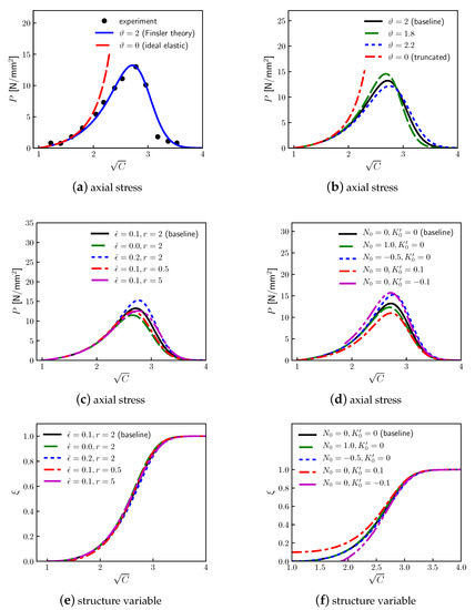
Figure 2. Extension and tearing of skin for the imposed axial stretch ratio $\sqrt{C}$, 1D model: (a) stress P comparison with data [74] (see text Section 4.5.1 for the definition of experimental stretch ratio) of Finsler model (baseline) and ideal nonlinear elasticity (null structure change) (b) effect on stress P of energy degradation exponent $\vartheta$ with $\widehat{ϵ}=0.1$, $r=2$, $N_0=0$, and $K_0^{\prime }=0$ (c) effect on stress P of Finsler metric scaling $\widehat{ϵ}=\frac{k}{r}$ and r with $\vartheta =2$, $N_0=0$, and $K_0^{\prime }=0$ (d) effect on stress P of nonlinear connection $N_0$ and linear connection $K_0^{\prime }$ with $\vartheta =2$, $\widehat{ϵ}=0.1$, and $r=2$ (e) effect on the internal structure $\xi =D/l$ of Finsler metric scaling $\widehat{ϵ}=\frac{k}{r}$ and r with $\vartheta =2$, $N_0=0$, and $K_0^{\prime }=0$ (f) effect on the internal structure $\xi =D/l$ of nonlinear connection $N_0$ and linear connection $K_0^{\prime }$ with $\vartheta =2$, $\widehat{ϵ}=0.1$, and $r=2$.

Table 1. Baseline model parameters for rabbit skin tissue: 1D and 2D theories.

Parameter	Units	Definition	Value (1D)	Value (2D)
l	mm	length scale	0.04	0.04
k	⋯	metric scaling factor	0.2	0.2
m	⋯	metric scaling factor	⋯	0.3
r	⋯	metric scaling exponent	2	2
${\mu }_0$	N/mm${}^2$	shear modulus (axial 1D)	0.2	0.2
${\kappa }_0$	N/mm${}^2$	bulk modulus (${\kappa }_0=k_0{\mu }_0$)	⋯	1.2
$a_1$	⋯	nonlinear elastic constant	2.8	2.8
$a_2$	⋯	nonlinear elastic constant	⋯	6
$b_1$	⋯	nonlinear elastic constant	0.055	0.055
$b_2$	⋯	nonlinear elastic constant	⋯	0.17
$\vartheta$	⋯	degradation exponent	2	2
$\varsigma$	⋯	degradation exponent	⋯	2
${{\rm Y}}_0$	mJ/mm${}^2$	isotropic surface energy	0.47	0.47
${\gamma }_{\xi }$	⋯	anisotropic energy factor	⋯	1
${\gamma }_{\eta }$	⋯	anisotropic energy factor	⋯	0.84

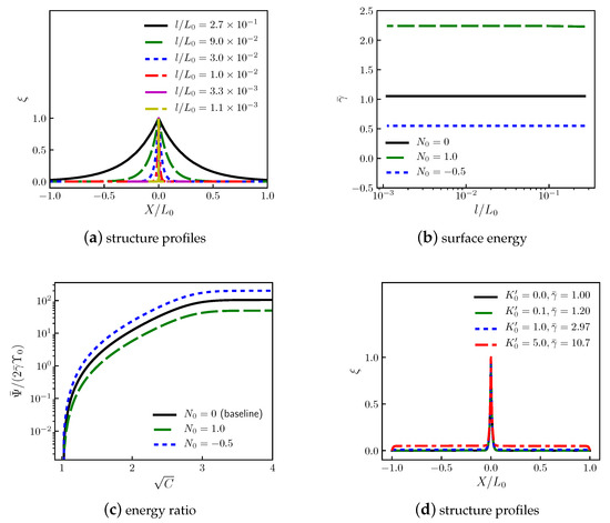
Figure 3. Extension and tearing of skin, 1D model: (a) Stress-free solution for the internal state profile (baseline parameters, $N_0=0$); (b) Normalized surface energy for rupture versus regularization length; (c) Ratio of homogeneous energy to energy for stress-free localized rupture; (d) Stress-free solution, $\widehat{ϵ}=0$, $l/L_0={10}^{-2}$, heterogeneous connection $\overline{K}\left(X\right)$.

Remark 39. 

The ideal elastic solution ($\xi =0$) is shown for comparison. Excluding structure evolution corresponding to collagen fiber rearrangements, sliding, and breakage, the model is too stiff relative to the data for which such microscopic mechanisms have been observed [74]. The ideal elastic model is unable to replicate the linearizing, softening, and failure mechanisms with increasing stretch $\sqrt{C}$ reported in experiments on the skin and other soft tissues [63,64,68,74,87].

In Figure 2b, the effects of $\vartheta$ on P are revealed for $\widehat{ϵ}=0.1$, $r=2$, $N_0=0$, and $K_0^{\prime }=0$, noting $\vartheta =0$ produces the ideal nonlinear elastic solution ${\xi }_{\mathrm{H}}=0$ in (142). Peak stress increases with decreasing $\vartheta$; the usual choice from phase-field theory $\vartheta =2$ provides close agreement with data in Figure 2a. In Figure 2c, the effects of Finsler metric scaling factors $\widehat{ϵ}=\frac{k}{r}$ and r on stress P are demonstrated, where, at fixed r, peak stress increases (decreases) with increasing (decreasing) $\widehat{ϵ}$ and k. Baseline choices $\widehat{ϵ}=0.1$ and $r=2$ furnish agreement with the experiment in Figure 2a. A remnant strain of 0.1 is of the same order of magnitude observed in cyclic loading experiments [72,78]. Complementary effects on the evolution of the structure versus stretch are shown in Figure 2e: modest changes in $\xi$ produce significant changes in P. In Figure 2d, the effects of connection coefficients $N_0$ and $K_0^{\prime }$ are revealed, holding material parameters at their baseline values in Table 1. For this homogeneous problem, maximum P decreases with increasing $N_0$ and $K_0^{\prime }$. The corresponding evolution of $\xi$ is shown in Figure 2f. When $K_0^{\prime }<0$, a viable solution ${\xi }_{\mathrm{H}}\in [0,1]$ exists only for $\sqrt{C}>1$.

The total energy per unit cross-sectional area of the specimen is $\overline{\Psi }$, found upon integration of $\psi (C_{\mathrm{H}},{\xi }_{\mathrm{H}})$ in (113) on $\mathcal{M}$ with the local element of volume $\mathrm{d}V=\sqrt{G\left({\xi }_{\mathrm{H}}\right)}\mathrm{d}X$:

$$\begin{array}{cc}\hfill \frac{\overline{\Psi }}{L_0}={\mu }_0& \left[{(1-{\xi }_{\mathrm{H}})}^{\vartheta }\{{(\sqrt{C_{\mathrm{H}}}-1)}^2+\frac{a_1}{2b_1}\left[\exp \left\{b_1{(C_{\mathrm{H}}-1)}^2\right\}-1\right]\}+\frac{{\xi }_{\mathrm{H}}^2}{A_0}\right]\hfill \\ & \times \exp \left(\frac{k}{r}{\xi }_{\mathrm{H}}^r\right).\hfill \end{array}$$

(143)

4.5.2. Stress-Free States

The stress-free solutions of Section 4.3.2 are applied to evaluate the remaining unknown parameters l and ${{\rm Y}}_0$, given ${\mu }_0$ and $A_0$ from Section 4.5.2. Assume the specimen tears completely at its midpoint at $X=0$, such that $\xi \left(0\right)=1$. No load is supported anywhere, and only rigid body motion is possible at other locations X where $\xi \left(X\right)>0$. Assume the specimen is clamped at its ends where it is gripped, such that $\xi (-L_0)=\xi \left(L_0\right)=0$. Symmetry conditions $\xi (-X)=\xi \left(X\right)$ are imposed, with ${\xi }^{\prime }\left(0\right)$ discontinuous, such that a solution needs to be calculated only for the half-space $X\in [0,L_0]$.

First, let $\overline{K}=l\widehat{K}=0$, so that (133) holds. Assume $c_1=0$ corresponding to ${\xi }^{\prime }=0$ where $\xi =0$ since the anti-derivative in (132) vanishes at $\xi =0$ when $\lambda ={\xi }^2,$$\chi =k{\xi }^{r-1},r>0$. It is verified a posteriori [55,59,62] that this closely approximates true boundary conditions $\xi (\pm L_0)=0$ as well as ${\xi }^{\prime }(\pm L_0)=0$ for $L_0\gg l$. Then the physically valid (negative) root for the half-domain giving $X\ge 0$ in (133) becomes, with (137) and (139),

$$\begin{array}{c}\hfill \frac{X\left(\xi \right)}{L_0}=-\frac{l}{L_0}\sqrt{1+N_0}{\int }_{z=1}^{z=\xi }\frac{\mathrm{d}z}{z\sqrt{1+2k{z}^r/\left[(1+N_0)(2+r)\right]}}.\end{array}$$

(144)

The lower limit follows from $X\left(1\right)=0$, obviating $c_2$ in (133). Analytical solution $\xi =argX\left(\xi \right)$ is exact, but it is most easily evaluated by quadrature when k is nonzero, decrementing z from 1 to 0 in small negative steps. The profile of $\xi \left(X\right)$ depends on $X/L_0$ and $l/L_0$, but not l or $L_0$ individually.

Remark 40. 

This new 1D solution, (144), agrees with more specific solutions derived in past work: $N_0=0$ and $r=1$ [55,56] with slight correction [59] and $N_0=0$ and $r=2$ [59].

Normalized surface energy per two-sided cross-sectional area, $\overline{\gamma }$, is obtained by integration of $\psi =\Lambda$ in (113) over $\mathcal{M}$:

$$\begin{array}{cc}\hfill \overline{\gamma }& =\frac{1}{2{{\rm Y}}_0}{\int }_{-L_0}^{L_0}\psi \sqrt{G}\mathrm{d}X\hfill \\ & =\frac{1}{2l}{\int }_{-L_0}^{L_0}\{{\xi }^2+(1+N_0)l{\xi }^{\prime }[2\widehat{K}+(1+N_0)l{\xi }^{\prime }]\}\exp \left[(k/r){\xi }^r\right]\mathrm{d}X.\hfill \end{array}$$

(145)

This energy likewise depends on $l/L_0$ but not l or $L_0$ individually. Baseline values of k and r are now taken from Table 1. The solution (144) is shown for $N_0=0$ and different $l/L_0$ in Figure 3a. The smaller (larger) the regularization length ratio $l/L_0$, the sharper (more diffuse) the zone centered at the midpoint of the domain over which prominent structure changes occur.

The normalized energy density (145) is shown in Figure 3b versus $l/L_0$ for several $N_0$. Increasing $N_0$ increases this energy, as might be anticipated from (113) with (114) when $\widehat{K}=0$. A stress-free ruptured state is energetically favorable to a stressed homogeneous state (§4.5.1) from applied deformation $C_{\mathrm{H}}$ when $\overline{\Psi }>2\overline{\gamma }{{\rm Y}}_0$, with $\overline{\Psi }$ given by (143). The ratio $\overline{\Psi }/\left(2\overline{\gamma }{{\rm Y}}_0\right)$ is shown in Figure 3c versus $\sqrt{C}=\sqrt{C_{\mathrm{H}}}$ with $l/L_0={10}^{-2}$ and several $N_0$, recalling $K_0^{\prime }=0$. Increasing $N_0$ increases $\overline{\gamma }$, reducing $\overline{\Psi }/\left(2\overline{\gamma }{{\rm Y}}_0\right)$. For cases in Figure 3a–c, $\xi (\pm L_0)<{10}^{-8}$ and $|l{\xi }^{\prime }(\pm L_0)|<{10}^{-8}$ are observed for $l/L_0\le 0.03$, verifying $c_1=0$ in (133) and (144) under this length constraint.

The remaining parameters l and ${{\rm Y}}_0$ are now quantified. To match the measured energy release rate ${\mathsf{J}}_{\mathrm{C}}$ (i.e., toughness) of skin, $2\overline{\gamma }{{\rm Y}}_0\approx {\mathsf{J}}_{\mathrm{C}}$. Let $L_0=4$ mm, the span of specimens [74] whose data are represented in Figure 2a. Then $l/L_0={10}^{-2}\Rightarrow l=40\mathsf{\mu }$m is more than sufficiently small to adhere to the aforementioned boundary constraints (i.e., $c_1=0$) while providing a damage profile of intermediate diffusivity in Figure 3a. This value of l then gives ${{\rm Y}}_0=\frac{{\mu }_{0}l}{2A_0}=0.47$ kJ/m${}^2$ (Table 1).

Remark 41. 

Along with the choice $N_0=0$, the Finsler model with the full set of baseline parameters in Table 1 produces $\overline{\gamma }\approx 1$ in Figure 3b and $2\overline{\gamma }{{\rm Y}}_0=1.0$ kJ/m${}^2$, in concurrence with experimental data: $0.5\lesssim {\mathsf{J}}_{\mathrm{C}}\lesssim 2.5$ kJ/m${}^2$ [73,99,113]. Value $l=40\mathsf{\mu }$m is between $4\times$ and $40\times$ the collagen fiber diameter [68,69,74]. Although not shown in Figure 3b, increasing $\widehat{ϵ}=\frac{k}{r}$ from 0.1 to 0.2 at $\vartheta =r=2$ with $N_0^{\prime }=K_0^{\prime }=0$ and $l/L_0={10}^{-2}$ increases effective toughness to $2\overline{\gamma }{{\rm Y}}_0=1.02$ kJ/m${}^2$. Under the same conditions, reducing $\widehat{ϵ}$ to 0 diminishes the predicted toughness to $2\overline{\gamma }{{\rm Y}}_0=0.94$ kJ/m${}^2$.

Finally, let $k=0$ but permit nonzero $\overline{K}\left(X\right)=l\widehat{K}\left(X\right)$, such that (135) applies. As an example, let $\overline{K}=-K_0^{\prime }l·(1-X/L_0)$ for $X\in [0,L_0]$ and $\overline{K}=K_0^{\prime }l·(1+X/L_0)$ for $X\in [-L_0,0)$. Boundary conditions $\xi \left(0\right)=1$ and $\xi (\pm L_0)=0$ still apply, as does symmetry relation $\xi \left(X\right)=\xi (-X)$. From (139), ${\omega }_1=1$ and ${\omega }_0=0$. For the whole domain $X\in [-L_0,L_0]$, ${\overline{K}}^{\prime }=K_0^{\prime }l/L_0=\mathrm{constant}$, and simply ${\xi }_{\mathrm{p}}=K_0^{\prime }l/L_0$. Then (135) gives

$$\begin{array}{cc}\hfill & \xi \left(X\right)=c_1\exp [X/\left\{l\sqrt{1+N_0}\right\}]+c_2\exp [-X/\left\{l\sqrt{1+N_0}\right\}]+K_0^{\prime }l/L_0,\hfill \\ \hfill & c_1=1-c_2-K_0^{\prime }l/L_0=\frac{-K_0^{\prime }l/L_0-[1-K_0^{\prime }l/L_0]\exp [-L_0/\left\{l\sqrt{1+N_0}\right\}]}{\exp [L_0/\left\{l\sqrt{1+N_0}\right\}]-\exp [-L_0/\left\{l\sqrt{1+N_0}\right\}]}.\hfill \end{array}$$

(146)

Profiles of $\xi \left(X\right)$ are shown in Figure 3d for $K_0^{\prime }\ge 0$ with baseline $l/L_0={10}^{-2}$. Normalized surface energy $\overline{\gamma }$ from (145) is reported in Figure 3d for each case, recalling $\widehat{ϵ}=k=0$ produces Riemannian (Euclidean) metric $G=1$. Setting $K_0^{\prime }>0$ increases $\overline{\gamma }$ for this problem. Setting $K_0^{\prime }<0$ reduces $\overline{\gamma }$ and produces a physically invalid solution (not shown in Figure 3d) in (146): $\xi <0$ on part of $\mathcal{M}$.

5. Two-Dimensional Base Manifold

The framework of Section 2 and Section 3 is applied for $n=2$: a 2D base manifold $\mathcal{M}$. In Section 5.1, geometry and kinematics are presented. Governing equations are derived in Section 5.2. Solutions are considered for general problem classes in Section 5.3. Constitutive functions for an orthotropic 2D patch of skin under planar deformations are assigned in Section 5.4. Solutions for stretching and tearing are presented in Section 5.5.

5.1. Geometry and Kinematics

Reference coordinates are Cartesian (i.e., orthogonal): $\{X^1,X^2\}$. A reference domain $\{\mathcal{M}:X^1\in [-L_0,L_0],X^2\in [-W_0,W_0]\}$ is considered, where the total area relative to a Euclidean metric is $4L_0{W}_0$, and boundary $\partial \mathcal{M}$ is the edges $(X^1,X^2)=(\pm L_0,\pm W_0)$. The referential internal state vector has coordinates $\{D^1,D^2\}$, both with physical units of length. Spatial coordinates are Cartesian $\{x^1,x^2\}$ and $\{d^1,d^2\}$. A normalization constant (i.e., regularization length) is l, with a physically meaningful domain assumed as $D^A\in [0,l]$ ($A=1,2$). With notation $f(X,D)=f(X^A,D^B)$, dimensionless order parameters are, with (68) and (70) invoked,

$$\xi \left(X\right)=\frac{D^1\left(X\right)}{l}=\frac{d^1\left(\phi \left(X\right)\right)}{l},\eta \left(X\right)=\frac{D^2\left(X\right)}{l}=\frac{d^2\left(\phi \left(X\right)\right)}{l},l>0.$$

(147)

Physically meaningful domains are $\xi \in [0,1]$ and $\eta \in [0,1]$. For 2D manifolds with Cartesian base coordinates, $\{X^1,X^2\}$ and $\{x^1,x^2\}$, the following metrics apply from (73) and (74):

$${\overline{G}}_{AB}={\delta }_{AB},{\overline{g}}_{ab}={\delta }_{ab};G_{AB}(X,D)={\widehat{G}}_{AB}\left(D\right),g_{ab}(x,d)={\widehat{g}}_{ab}\left(d\right).$$

(148)

Herein, the following constraint is imposed:

$${\widehat{g}}_{ab}\left(d\left(\phi \left(X\right)\right)\right)={\delta }_a^A{\delta }_b^B{\widehat{G}}_{AB}\left(D\left(X\right)\right)\leftrightarrow g_{ab}(\xi ,\eta )={\delta }_a^A{\delta }_b^B{G}_{AB}(\xi ,\eta ),$$

(149)

making $\mathfrak{m}$ and $\mathcal{M}$ isometric when ${\varphi }^a\left(X\right)={\delta }_A^a{X}^A+c_0^a\iff F_A^a={\delta }_A^a$ regardless of $\{\xi ,\eta \}$ at $x=\phi \left(X\right)$.

Remark 42. 

Equation (149) may be removed in other settings to directly model residual stress (e.g., Appendix B), but all residual stresses are not necessarily eliminated with (149) in place.

Although other non-trivial forms are admissible (e.g., Section 4.1), assume nonlinear $N_B^A$ and linear $K_{BC}^A$ connections vanish:

$$N_B^A=0\Rightarrow N_b^a={\delta }_A^a{N}_B^A{\left(F^{-1}\right)}_b^B=0,K_{BC}^A=0.$$

(150)

The $K_{bc}^a$ do not affect the governing equations to be solved later, so they are unspecified.

Applying (71) and (147)–(150),

$${\delta }_A{G}_{BC}={\partial }_A{G}_{BC}-N_A^D{\overline{\partial }}_D{G}_{BC}=0\Rightarrow {\Gamma }_{BC}^A=0,{\delta }_a{g}_{bc}=0\Rightarrow {\Gamma }_{bc}^a=0,$$

(151)

$${\chi }_A(\xi ,\eta )=l{C}_{AB}^B(\xi ,\eta )=l{\overline{\partial }}_A\{ln\sqrt{G(\xi ,\eta )}\};l{\overline{\partial }}_1(·)=\partial (·)/\partial \xi ,l{\overline{\partial }}_2(·)=\partial (·)/\partial \eta .$$

(152)

The deformation gradient, deformation tensor, Jacobian determinant, and director gradient are, respectively,

$$F_A^a=\frac{\partial {\phi }^a}{\partial X^A},C_B^A=G^{AC}{g}_{bc}{F}_B^b{F}_C^c=G^{AC}{F}_C^c{\delta }_c^F{G}_{FE}{\delta }_b^E{F}_B^b,J=det\left(F_A^a\right)=\sqrt{det\left(C_B^A\right)},$$

(153)

$$D_{|B}^A={\delta }_B{D}^A+K_{BC}^A{D}^C={\partial }_B{D}^A;D_{|A}^1=l{\partial }_A\xi ,D_{|A}^2=l{\partial }_A\eta .$$

(154)

Unless $F_A^a$ and $G_{AB}$ are diagonal, $\mathit{C}$ and $\overline{\mathit{C}}$ can differ. From (75) and (76),

$${\overline{C}}_B^A={\delta }^{AC}{\overline{C}}_{CB}={\delta }^{AC}{\delta }_{bc}{F}_B^b{F}_C^c,\overline{J}=\sqrt{det\left({\overline{C}}_B^A\right)}=J.$$

(155)

5.2. Governing Equations

A generic energy density is chosen and equilibrium equations are derived for the 2D case of Section 5.1.

5.2.1. Energy Density

For the present case, dependencies on $D^A$ and $D_{|B}^A$ are suitably represented by ($\xi ,\eta$) and $({\partial }_A\xi ,{\partial }_A\eta )$ of (147) and (154). The functional form of (94) is invoked without explicit X dependency, whereby

$$\psi =\overline{\psi }({\overline{C}}_{AB},\xi ,\eta ,{\partial }_A\xi ,{\partial }_A\eta ).$$

(156)

Henceforth, in Section 5, the over-bar is dropped from $\psi$ to lighten the notation. Let ${\mu }_0$ denote a constant that will later be associated with a shear modulus, with units of energy density.

Remark 43. 

For comparison with experiments in ambient 3-space, ${\mu }_0$ has units of energy per unit 3D volume, so $\Psi ={\int }_{\mathcal{M}}\psi d\Omega$ is the energy per unit thickness, normal to the $X^1$ and $X^2$.

Let ${{\rm Y}}_0$ denote a constant related to the surface energy with units of energy per unit (e.g., 2D fixed cross-sectional) area, and  ${\gamma }_{\xi }$ and ${\gamma }_{\eta }$ denote two dimensionless constants. Let W be the strain energy density and $\Lambda$ denote energy density associated with the microstructure. Let w denote a dimensionless strain energy function (embedding possible degradation), $\lambda$ and $\nu$ denote dimensionless phase energy functions, $\iota$ denote a dimensionless gradient energy function that is assigned a sum of quadratic forms, and ${\nabla }_0(·)=\frac{\partial }{\partial \mathit{X}}(·)$ denote the partial material gradient. Free energy (156) is prescribed in intermediate functional form, as

$$\begin{array}{cc}\hfill \psi (\overline{\mathit{C}},\xi ,\eta ,{\nabla }_0\xi ,{\nabla }_0\eta )& =W(\overline{\mathit{C}},\xi ,\eta )+\Lambda (\xi ,\eta ,{\nabla }_0\xi ,{\nabla }_0\eta )\hfill \\ & =\frac{{\mu }_0}{2}w(\overline{\mathit{C}},\xi ,\eta )+\frac{{{\rm Y}}_0}{l}[{\gamma }_{\xi }\lambda \left(\xi \right)+{\gamma }_{\eta }\nu \left(\eta \right)+\iota ({\nabla }_0\xi ,{\nabla }_0\eta )],\hfill \end{array}$$

(157)

$$\iota ={\gamma }_{\xi }|l{\nabla }_0{\xi |}^2+{\gamma }_{\eta }{l}^2{|l{\nabla }_0\eta |}^2=l^2{\delta }^{AB}({\gamma }_{\xi }{\partial }_A\xi {\partial }_B\xi +{\gamma }_{\eta }{\partial }_A\eta {\partial }_B\eta ).$$

(158)

Note that $\iota (0,0)=0$. Therefore, for null ground-state energy density, $\psi$, and stress, $P_a^A$,

$$w({\delta }_{AB},\xi ,\eta )=0,\frac{\partial w}{\partial {\overline{C}}_{AB}}({\delta }_{AB},\xi ,\eta )=0;\lambda \left(0\right)=\nu \left(0\right)=0.$$

(159)

Convexity and material symmetry are addressed in Section 5.4.2.

Applying (96), thermodynamic forces of (85) are

$$P_a^A=\frac{\partial \psi }{\partial F_A^a}=2{\delta }_{ab}{F}_B^b\frac{\partial \psi }{\partial {\overline{C}}_{AB}}={\mu }_0{\delta }_{ab}{F}_B^b\frac{\partial w}{\partial {\overline{C}}_{AB}},$$

(160)

$$\begin{array}{cc}\hfill Q_1& =\frac{1}{l}\frac{\partial \psi }{\partial \xi }=\frac{{{\rm Y}}_0}{l^2}\left(A_0\frac{\partial w}{\partial \xi }+{\gamma }_{\xi }\frac{\mathrm{d}\lambda }{\mathrm{d}\xi }\right),\hfill \\ \hfill Q_2& =\frac{1}{l}\frac{\partial \psi }{\partial \eta }=\frac{{{\rm Y}}_0}{l^2}\left(A_0\frac{\partial w}{\partial \eta }+{\gamma }_{\eta }\frac{\mathrm{d}\nu }{\mathrm{d}\eta }\right);A_0=\frac{{\mu }_{0}l}{2{{\rm Y}}_0},\hfill \end{array}$$

(161)

$$\begin{array}{cc}\hfill Z_1^A& =\frac{\partial \psi }{\partial D_{|A}^1}=\frac{{{\rm Y}}_0}{l^2}\frac{\partial \iota }{\partial \left({\partial }_A\xi \right)}=2{{\rm Y}}_0{\gamma }_{\xi }{\delta }^{AB}{\partial }_B\xi ,\hfill \\ \hfill Z_2^A& =\frac{\partial \psi }{\partial D_{|A}^2}=\frac{{{\rm Y}}_0}{l^2}\frac{\partial \iota }{\partial \left({\partial }_A\eta \right)}=2{{\rm Y}}_0{\gamma }_{\eta }{\delta }^{AB}{\partial }_B\eta .\hfill \end{array}$$

(162)

The source term in (78) manifests from changes in energy proportional to changes in the local referential volume form (e.g., local volume changes from damage, treated analogously to an energy source from tissue growth (Appendix B)):

$$R_A=\beta \psi {\overline{\partial }}_A(ln\sqrt{G})=\frac{\beta }{l}\psi {\chi }_A,(\beta =\mathrm{constant};A=1,2).$$

(163)

5.2.2. Linear Momentum

Linear momentum balance, (87) or (90), invokes relations in Section 5.1 and Section 5.2.1,

$$\begin{array}{cc}\hfill {\mu }_0{\delta }_{ab}& \left[\frac{{\partial }^2{\phi }^b}{\partial X^A\partial X^B}\frac{\partial w}{\partial {\overline{C}}_{AB}}+\frac{\partial {\phi }^b}{\partial X^B}\left(\frac{{\partial }^{2}w}{\partial {\overline{C}}_{AB}\partial X^A}+\frac{{\partial }^{2}w}{\partial {\overline{C}}_{AB}\partial \xi }\frac{\partial \xi }{\partial X^A}+\frac{{\partial }^{2}w}{\partial {\overline{C}}_{AB}\partial \eta }\frac{\partial \eta }{\partial X^A}\right)\right]\hfill \\ & =-{\mu }_0{\delta }_{ab}\frac{\partial {\phi }^b}{\partial X^B}\frac{\partial w}{\partial {\overline{C}}_{AB}}\left[\frac{\partial }{\partial \xi }\left(ln\sqrt{G}\right)\frac{\partial \xi }{\partial X^A}+\frac{\partial }{\partial \eta }\left(ln\sqrt{G}\right)\frac{\partial \eta }{\partial X^A}\right].\hfill \end{array}$$

(164)

Remark 44. 

For nonzero ${\mu }_0$, (164) is two coupled nonlinear PDEs ($a=1,2$) in four field variables: ${\phi }^1\left(X\right)$, ${\phi }^2\left(X\right)$, $\xi \left(X\right)$, and $\eta \left(X\right)$.

5.2.3. Micro-Momentum

The state-space equilibrium conditions (88) or (91), utilizing the relations from Section 5.1 and Section 5.2.1, and dividing by $2{{\rm Y}}_0$, yield the following two equations:

$$\begin{array}{cc}\hfill {\gamma }_{\xi }& {\delta }^{AB}\frac{{\partial }^2\xi }{\partial X^A\partial X^B}+\left(1-\frac{\alpha -\beta }{2}\right){\gamma }_{\xi }{\delta }^{AB}\frac{\partial }{\partial \xi }\left(ln\sqrt{G}\right)\frac{\partial \xi }{\partial X^A}\frac{\partial \xi }{\partial X^B}-\frac{{\gamma }_{\xi }}{2l^2}\frac{\mathrm{d}\lambda }{\mathrm{d}\xi }\hfill \\ & +{\gamma }_{\xi }{\delta }^{AB}\frac{\partial }{\partial \eta }\left(ln\sqrt{G}\right)\frac{\partial \xi }{\partial X^A}\frac{\partial \eta }{\partial X^B}-\left(\frac{\alpha -\beta }{2}\right){\gamma }_{\eta }{\delta }^{AB}\frac{\partial }{\partial \xi }\left(ln\sqrt{G}\right)\frac{\partial \eta }{\partial X^A}\frac{\partial \eta }{\partial X^B}\hfill \\ & -\left(\frac{\alpha -\beta }{2l^2}\right)\frac{\partial }{\partial \xi }\left(ln\sqrt{G}\right)[{\gamma }_{\xi }\lambda +{\gamma }_{\eta }\nu ]=\frac{A_0}{2l^2}\left[\frac{\partial w}{\partial \xi }+(\alpha -\beta )\frac{\partial }{\partial \xi }\left(ln\sqrt{G}\right)w\right],\hfill \end{array}$$

(165)

$$\begin{array}{cc}\hfill {\gamma }_{\eta }& {\delta }^{AB}\frac{{\partial }^2\eta }{\partial X^A\partial X^B}+\left(1-\frac{\alpha -\beta }{2}\right){\gamma }_{\eta }{\delta }^{AB}\frac{\partial }{\partial \eta }\left(ln\sqrt{G}\right)\frac{\partial \eta }{\partial X^A}\frac{\partial \eta }{\partial X^B}-\frac{{\gamma }_{\eta }}{2l^2}\frac{\mathrm{d}\nu }{\mathrm{d}\eta }\hfill \\ & +{\gamma }_{\eta }{\delta }^{AB}\frac{\partial }{\partial \xi }\left(ln\sqrt{G}\right)\frac{\partial \eta }{\partial X^A}\frac{\partial \xi }{\partial X^B}-\left(\frac{\alpha -\beta }{2}\right){\gamma }_{\xi }{\delta }^{AB}\frac{\partial }{\partial \eta }\left(ln\sqrt{G}\right)\frac{\partial \xi }{\partial X^A}\frac{\partial \xi }{\partial X^B}\hfill \\ & -\left(\frac{\alpha -\beta }{2l^2}\right)\frac{\partial }{\partial \eta }\left(ln\sqrt{G}\right)[{\gamma }_{\xi }\lambda +{\gamma }_{\eta }\nu ]=\frac{A_0}{2l^2}\left[\frac{\partial w}{\partial \eta }+(\alpha -\beta )\frac{\partial }{\partial \eta }\left(ln\sqrt{G}\right)w\right].\hfill \end{array}$$

(166)

Remark 45. 

For nonzero ${{\rm Y}}_0$, (165) and (166) are two coupled nonlinear PDEs in four field variables: ${\phi }^1\left(X\right)$, ${\phi }^2\left(X\right)$, $\xi \left(X\right)$, and $\eta \left(X\right)$, where derivatives of ${\phi }^1\left(X\right)$ and ${\phi }^2\left(X\right)$ enter w on the right sides via ${\overline{C}}_{AB}={\partial }_A{\phi }^a{\delta }_{ab}{\partial }_B{\phi }^b$. For the special case ${{\rm Y}}_0=0$, the left sides of (165) and (166) vanish, whereas for ${\mu }_0=0$, the right sides vanish.

5.3. General Solutions

5.3.1. Homogeneous Fields

Cases for which $\xi \left(X\right)\to {\xi }_{\mathrm{H}}=\mathrm{constant}$ and $\eta \left(X\right)\to {\eta }_{\mathrm{H}}=\mathrm{constant}$ at all points $X\in \mathcal{M}$ are examined. The former constants may differ: ${\xi }_{\mathrm{H}}\ne {\eta }_{\mathrm{H}}$ in general. The notation $f_{\mathrm{H}}\left(X\right)=f(X,{\xi }_{\mathrm{H}},{\eta }_{\mathrm{H}})$ is applied, and ${\mu }_0>0$ is imposed. Then (160) and (164) reduce to

$$\begin{array}{cc}\hfill \frac{\partial P_a^A}{\partial X^A}={\mu }_0{\delta }_{ab}& \left[\frac{{\partial }^2{\phi }^b}{\partial X^A\partial X^B}\frac{\partial w}{\partial {\overline{C}}_{AB}}+\frac{\partial {\phi }^b}{\partial X^B}\frac{{\partial }^{2}w}{\partial {\overline{C}}_{AB}\partial X^A}\right]=0\hfill \\ & \Rightarrow {\left(P_{\mathrm{H}}\right)}_a^A=\frac{{\mu }_0}{2}{\left(\frac{\partial w}{\partial F_A^a}\right)}_{\mathrm{H}}=\mathrm{constant}.\hfill \end{array}$$

(167)

This should be satisfied for any homogeneous $F_A^a={\left(F_{\mathrm{H}}\right)}_A^a$ for which ${\partial }^2{\phi }^a/\partial X^A\partial X^B=0$. The micro-momentum conservation laws (165) and (166) become

$$\begin{array}{c}\hfill -{\gamma }_{\xi }\frac{\mathrm{d}\lambda }{\mathrm{d}\xi }-\left(\alpha -\beta \right)\frac{\partial }{\partial \xi }\left(ln\sqrt{G}\right)[{\gamma }_{\xi }\lambda +{\gamma }_{\eta }\nu ]=A_0\left[\frac{\partial w}{\partial \xi }+(\alpha -\beta )\frac{\partial }{\partial \xi }\left(ln\sqrt{G}\right)w\right],\end{array}$$

(168)

$$\begin{array}{c}\hfill -{\gamma }_{\eta }\frac{\mathrm{d}\nu }{\mathrm{d}\eta }-\left(\alpha -\beta \right)\frac{\partial }{\partial \eta }\left(ln\sqrt{G}\right)[{\gamma }_{\xi }\lambda +{\gamma }_{\eta }\nu ]=A_0\left[\frac{\partial w}{\partial \eta }+(\alpha -\beta )\frac{\partial }{\partial \eta }\left(ln\sqrt{G}\right)w\right],\end{array}$$

(169)

wherein $\lambda ={\lambda }_{\mathrm{H}}$, $\nu ={\nu }_{\mathrm{H}}$, ${(\frac{\partial }{\partial \xi }ln\sqrt{G})}_{\mathrm{H}}$, and ${(\frac{\partial }{\partial \eta }ln\sqrt{G})}_{\mathrm{H}}$ are all algebraic functions of $({\xi }_{\mathrm{H}},{\eta }_{\mathrm{H}})$, while $w=w_{\mathrm{H}}$, ${\left(\frac{\partial }{\partial \xi }w\right)}_{\mathrm{H}}$, and ${\left(\frac{\partial }{\partial \eta }w\right)}_{\mathrm{H}}$ are algebraic functions of $({\xi }_{\mathrm{H}},{\eta }_{\mathrm{H}},{\left(F_{\mathrm{H}}\right)}_A^a)$.

Remark 46. 

The homogeneous equilibrium is satisfied by the six algebraic equations (167) ($a,A=1,2$), (168), and (169) in ten unknowns ${\left(P_{\mathrm{H}}\right)}_a^A$, ${\left(F_{\mathrm{H}}\right)}_A^a$, ${\xi }_{\mathrm{H}}$, ${\eta }_{\mathrm{H}}$. Given ${\left(P_{\mathrm{H}}\right)}_a^A$ or ${\left(F_{\mathrm{H}}\right)}_A^a$ as the mechanical loading, the remaining six unknowns can be obtained from a simultaneous solution. If ${\left(F_{\mathrm{H}}\right)}_A^a$ is imposed, (168) and (169) are two equations in ${\xi }_{\mathrm{H}}$, ${\eta }_{\mathrm{H}}$. Then (167) yields the remaining ${\left(P_{\mathrm{H}}\right)}_a^A$.

Remark 47. 

Essential boundary conditions for homogeneous states are $\xi ={\xi }_{\mathrm{H}}$ and $\eta ={\eta }_{\mathrm{H}}$, both $\forall X\in \partial \mathcal{M}$. Since $\xi$ and $\eta$ are constants, $Z_A^B=0$ by (162), so corresponding natural boundary conditions for forces conjugating to internal structure parameters in (89) are $z_A=Z_A^B{N}_B=0$.

5.3.2. Stress-Free States

Consider cases whereby $P_a^A=0\forall X\in \mathcal{M}$. Linear momentum conservation laws (87), (90), and (164), are trivially satisfied. Restrict ${\mu }_0>0$. Since $F_A^a$ is non-singular, (160) requires $\partial w/\partial {\overline{C}}_{AB}=0$. This is obeyed at ${\overline{C}}_{AB}={\delta }_{AB}$ via (159); thus, assume rigid body motion (i.e., ${\phi }^a=Q_A^a{X}^A+c_0^a$, with $Q_A^a$ constant and proper orthogonal and $c_0^a$ constant) whereby $w=0$ vanishes as well by (159).

Remark 48. 

General analytical solutions for stress-free states are not apparent without particular forms of functions $w({\overline{C}}_{AB},\xi ,\eta )$, $G(\xi ,\eta )$, $\lambda \left(\xi \right)$, $\nu \left(\eta \right)$, and values of ${\gamma }_{\xi }$, ${\gamma }_{\eta }$, $\alpha$, $\beta$, and l.

Remark 49. 

If $\partial w/\partial \xi =\partial w/\partial \eta =0$ for ${\overline{C}}_{AB}={\delta }_{AB}$, then the right sides of (165) and (166) vanish. Whether or not stress-free deformation states with ${\overline{C}}_{AB}\ne {\delta }_{AB}$ (e.g., locally) exist depends on w.

5.4. Constitutive Model

The framework is applied to a rectangular patch of skin loaded in the $X^1$-$X^2$ plane. A 2D theory (i.e., membrane theory) cannot distinguish between plane stress and plane strain conditions [115], nor can it account for out-of-plane anisotropy. Nonetheless, 2D nonlinear elastic models are widely used to represent soft tissues, including skin [68,89]. Thus, parameters entering the model (e.g., ${\mu }_0$, ${{\rm Y}}_0$) are particular to loading conditions and material orientations from experiments to which they are calibrated (e.g., here, plane stress).

Remark 50. 

In a purely 2D theory, incompressibility is often used for the 3D modeling of biological tissues [68,71,80,82] cannot be assumed since contraction under biaxial stretch is not quantified in a 2D theory. Incompressibility is also inappropriate if the material dilates due to damage.

The skin is treated as having orthotropic symmetry, with two constant orthogonal directions in the reference configuration denoted by unit vectors ${\mathit{n}}_1$ and ${\mathit{n}}_2$:

$${\mathit{n}}_1=n_1^A\frac{\delta }{\delta X^A},{\mathit{n}}_2=n_2^A\frac{\delta }{\delta X^A};n_i^A{\delta }_{AB}{n}_j^B={\delta }_{ij}(i,j=1,2).$$

(170)

Remark 51. 

The collagen fibers in the plane of the skin need not all align with ${\mathit{n}}_1$ or ${\mathit{n}}_2$, so long as orthotropic symmetry is respected. For example, each ${\mathit{n}}_i$ can bisect the alignments of two equivalent primary families of fibers in the skin whose directions are not necessarily orthogonal [71,92]. In such a case, ${\mathit{n}}_1$ is still a unit vector orthogonal to ${\mathit{n}}_2$; planar orthotropy is maintained with respect to reflections about both unit vectors ${\mathit{n}}_i$.

Remark 52. 

The internal structure variables $\xi =D^1/l$ and $\eta =D^2/l$ account for mechanisms that lead to softening and degradation under tensile load: fiber sliding, pull-out, and breakage of collagen fibers, and rupture of the elastin fibers and ground matrix. Each $D^A$ ($A=1,2$) is a representative microscopic sliding or separation distance in the ${\mathit{n}}_i{\delta }_A^i$ direction, with l the distance at which the material can no longer support tensile load along that direction.

Remark 53. 

In the cohesive zone interpretation, each $D^A$ is viewed as a crack-opening displacement for separation on a material surface (line in 2D) normal to ${\mathit{n}}_i{\delta }_A^i$.

Finslerian metrics $G_{AB}(\xi ,\eta )={\delta }_A^a{\delta }_B^b{g}_{ab}(\xi ,\eta )$ of §5.4.1 anisotropically rescale material and spatial manifolds $\mathcal{M}$ and $\mathfrak{m}$ due to microstructure changes in different directions. In the absence of damage, the nonlinear elastic potential of Section 5.4.2 refines a 3D model [71,82,83,92] to 2D.

5.4.1. Metrics

From (16), (48), (148), (149), and (153), the difference in squared lengths of line elements $\mathrm{d}\mathit{x}$ and $\mathrm{d}\mathit{X}$ is

$${(|\mathrm{d}\mathit{x}|}^2-{|\mathrm{d}\mathit{X}|}^2)(\mathit{F},\xi ,\eta )=[{\delta }_a^E{\delta }_b^F{G}_{EF}(\xi ,\eta )F_A^a{F}_B^b-G_{AB}(\xi ,\eta )]\mathrm{d}{X}^A\mathrm{d}{X}^B.$$

(171)

Remark 54. 

Local regions of $\mathcal{M}$ at X and $\mathfrak{m}$ at $x=\phi \left(X\right)$ are rescaled isometrically by components $G_{AB}(\xi \left(X\right),\eta \left(X\right))$. When $F_A^a={\delta }_A^a$, $|d\mathit{x}|=|d\mathit{X}|$ regardless of $G_{AB}$, $\xi$, or $\eta$. For degenerate Riemannian metrics $G_{AB}={\overline{G}}_{AB}={\delta }_{AB}$ and $g_{ab}={\overline{g}}_{ab}={\delta }_{ab}$, (171) becomes independent of ($\xi ,\eta$).

The Cartesian coordinate chart $\left\{X^A\right\}$ is prescribed such that $n_i^A={\delta }_i^A$ in (170); thus ${\mathit{n}}_1$ and ${\mathit{n}}_2$ are parallel to respective $X^1$ and $X^2$ directions on $\mathcal{M}$. Rescaling arises from changes in structure associated with degradation and damage in orthogonal directions, to which remnant strain contributions $\frac{1}{2}ln\left[G_{11}\left(\xi \right)\right]$ and $\frac{1}{2}ln\left[G_{22}\left(\eta \right)\right]$ can be linked. The metric tensor $G_{AB}$ is hereafter assigned specific exponential terms, generalizing the 1D form of Section 4.4.1 to an anisotropic 2D form appropriate for orthotropic symmetry:

$$\begin{array}{cc}\hfill \left[G_{AB}(\xi ,\eta )\right]=& \left[\begin{array}{cc}\exp \left(\frac{2k}{r}{\xi }^r\right)& 0\\ 0& \exp \left(\frac{2m}{r}{\eta }^r\right)\end{array}\right]\hfill \\ & \Rightarrow G(\xi ,\eta )=det\left[G_{AB}(\xi ,\eta )\right]=\exp \left(\frac{2}{r}[k{\xi }^r+m{\eta }^r]\right).\hfill \end{array}$$

(172)

For $\xi \in [0,1]$ and $\eta \in [0,1]$, two constants in (172) are k and m, and positive for expansion. A third constant $r>0$ modulates rates of change of $G_{11}\left(\xi \right)$ and $G_{22}\left(\eta \right)$ with respect to their arguments. Ratios are determined by remnant strain contributions at failure: ${\widehat{ϵ}}_{\xi }=\frac{k}{r}$ and ${\widehat{ϵ}}_{\eta }=\frac{m}{r}$. Values of k, m, and r are calibrated to data in Section 5.5.1. Isotropy arises in (172) when $\eta =\xi$ and $m=k$.

Remark 55. 

More general forms of $G_{AB}(\xi ,\eta )$, likely with more parameters, are possible; (172) is a simple form sufficient to address experimental observations for extension and tearing of skin.

From (172), non-vanishing components of Cartan’s tensor in (25) and (152) are

$$l{C}_{11}^1={\chi }_1=\frac{\partial }{\partial \xi }(ln\sqrt{G})=k{\xi }^{r-1},l{C}_{22}^2={\chi }_2=\frac{\partial }{\partial \eta }(ln\sqrt{G})=m{\eta }^{r-1}.$$

(173)

5.4.2. Nonlinear Elasticity

The nonlinear elasticity model generalizes that of Section 4.4.2 to a 2D base space $\mathcal{M}$ with the anisotropic Finsler metric depending on two structure variable components, $\xi$ and $\eta$ in normalized dimensionless form. For the 2D case, the material symmetry of Section 3.3.4 requires careful consideration. Here, the skin is treated as a planar orthotropic solid [68,75,89].

Viewing the $D^A$ as components of a material vector field, orthotropic symmetry suggests invariants ${\xi }^2$ and ${\eta }^2$. For physically admissible ranges $\xi \in [0,1]$ and $\eta \in [0,1]$, these can be replaced with $\xi$ and $\eta$. Viewing the $D_{|B}^A$, similarly, orthotropic symmetry permits a more general functional dependence than the sum of quadratic forms in $\iota$ of (157) and (158). However, the chosen form of $\iota$ in (158) allows for partial anisotropy, not inconsistent with orthotropy, when ${\gamma }_{\xi }$ and ${\gamma }_{\eta }$ differ. Thus, the structure-dependent contribution to $\psi$, $\Lambda l={{\rm Y}}_0({\gamma }_{\xi }\lambda +{\gamma }_{\eta }\nu +\iota )$, more specifically here

$$\lambda \left(\xi \right)={\xi }^2,\nu \left(\eta \right)={\eta }^2;\iota ({\nabla }_0\xi ,{\nabla }_0\eta )=l^2{\delta }^{AB}({\gamma }_{\xi }{\partial }_A\xi {\partial }_B\xi +{\gamma }_{\eta }{\partial }_A\eta {\partial }_B\eta ),$$

(174)

is consistent with material symmetry requirements. Strain energy density W in (157) is dictated by dimensionless function $w({\overline{C}}_{AB},\xi ,\eta )$. As per the above discussion, $\xi$ and $\eta$ are treated as scalar invariant arguments. A partial list of remaining invariants [82,91] of (99) for orthotropic symmetry of a 2D material entering w (and, thus, $\psi =\overline{\psi }$) is then deduced, applying $n_i^A={\delta }_i^A$ in (170),

$$\begin{array}{cc}\hfill {\overline{I}}_1& =\mathrm{tr}\overline{\mathit{C}}={\delta }^{AB}{\overline{C}}_{AB},{\overline{I}}_2=J^2=det\overline{\mathit{C}},\hfill \\ \hfill {\overline{I}}_3& ={\overline{C}}_{AB}{n}_1^A{n}_1^B={\overline{C}}_{11},{\overline{I}}_4={\overline{C}}_{AB}{n}_2^A{n}_2^B={\overline{C}}_{22}.\hfill \end{array}$$

(175)

Remark 56. 

As ${\mathit{n}}_1$ and ${\mathit{n}}_2$ are orthonormal, ${\overline{I}}_1={\overline{I}}_3+{\overline{I}}_4$, so one of ${\overline{I}}_1,{\overline{I}}_3,{\overline{I}}_4$ in (175) is redundant. Since $J\ge 1$, dependence on ${\overline{I}}_2={\overline{C}}_{11}{\overline{C}}_{22}-{\left({\overline{C}}_{12}\right)}^2$ can be replaced by J (or by ${\left({\overline{C}}_{12}\right)}^2$, given ${\overline{I}}_3,{\overline{I}}_4$).

The Euclidean metric ${\overline{G}}^{AB}={\delta }^{AB}$, rather than the Finsler metric $G^{AB}$, is used for scalar products in (174) and (175), consistent with (155). In 2-space, ${\overline{I}}_1$ and ${\overline{I}}_2$ are the complete set of isotropic invariants of $\overline{\mathit{C}}$. Two orthotropic invariants are ${\overline{I}}_3$ and ${\overline{I}}_4$; several higher-order invariants are admissible [82,91] but excluded here since (175) is sufficient for the present application. The dimensionless strain energy function entering (157) is prescribed specifically as

$$\begin{array}{cc}\hfill w({\overline{C}}_{AB},\xi ,\eta )& =\left[\frac{1}{J}({\overline{C}}_{11}+{\overline{C}}_{22})+k_0{(J-1)}^2-2\right]y_{\mu }(\xi ,\eta )\hfill \\ \hfill & +\left[\frac{a_1}{2b_1}\left(\exp \left\{b_1{({\overline{C}}_{11}-1)}^2\right\}-1\right)\right]\mathrm{H}({\overline{C}}_{11}-1)y_{\xi }\left(\xi \right)\hfill \\ \hfill & +\left[\frac{a_2}{2b_2}\left(\exp \left\{b_2{({\overline{C}}_{22}-1)}^2\right\}-1\right)\right]\mathrm{H}({\overline{C}}_{22}-1)y_{\eta }\left(\eta \right).\hfill \end{array}$$

(176)

Dimensionless constants are $k_0>0$, $a_1\ge 0$, $b_1>0$, $a_2\ge 0$, and $b_2>0$. Right-continuous Heaviside functions $\mathrm{H}\left(f\right)=1\forall f\ge 0,\mathrm{H}\left(f\right)=0\forall f<0$. Also, ${\mu }_0>0$ and ${{\rm Y}}_0>0$ are enforced in (157).

Remark 57. 

Potential w in (176) extends prior models for collagenous tissues [71,82,83,92] to include anisotropic structure changes. The first term on the right, linear in ${\overline{I}}_1/J$, and independent of volume change, accounts for isotropic shearing resistance of ground matrix and elastin. The resistance to volume (area) change is measured by the right-side second bracketed entry with $k_0$ being a dimensionless bulk (area) modulus finite for a 2D model; the dimensional bulk modulus ${\kappa }_0=k_0{\mu }_0$. Exponential terms account for stiffening from collagen fibers in orthogonal directions ${\mathit{n}}_i$. Heaviside functions prevent fibers from supporting compressive loads [82,116] since they would likely buckle.

Degradation functions are $y_{\mu }(\xi ,\eta )$, $y_{\xi }\left(\xi \right)$, and $y_{\eta }\left(\eta \right)$, where for the anisotropic theory,

$$y_{\mu }={(1-\xi )}^{\vartheta }{(1-\eta )}^{\varsigma }=y_{\xi }{y}_{\eta },y_{\xi }={(1-\xi )}^{\vartheta },y_{\eta }={(1-\eta )}^{\varsigma }.$$

(177)

Corresponding material constants are $\vartheta \in [0,\infty )$ and $\varsigma \in [0,\infty )$. Notice that matrix strain energy degrades equivalently with the increasing $\xi$ and $\eta$ via $y_{\mu }$, maintaining isotropy of the first term in (176). As collagen fibers debond, the ground matrix and elastic simultaneously weaken.

Remark 58. 

Choices $\vartheta =\varsigma =2$ are typical for phase-field fracture [98], although other values are possible for soft biologic tissues [95]. Setting $\vartheta =\varsigma =0$ implies null degradation (i.e., ideal elastic stress–stretch response).

Remark 59. 

When $\xi =\eta =0$, w of (176) is polyconvex [81,90], facilitating existence and uniqueness of solutions. Also, $\psi$ with (174), (176), and (177) obeys (159).

Stress components $P_a^A$ conjugating to $F_A^a={\partial }_A{\phi }^a$ are found from (100), (160), (176), and (177), while forces $Q_{1,2}$ conjugating to $\xi ,\eta$ are found from (161), (174), (176), and (177):

$$\begin{array}{cc}\hfill P_a^A/{\mu }_0=J^{-1}& [{\delta }_{ab}{\delta }^{AB}{F}_B^b-\frac{1}{2}{\overline{C}}_{BC}{\delta }^{BC}{\left(F^{-1}\right)}_a^A+k_0{J}^2(J-1){\left(F^{-1}\right)}_a^A]{(1-\xi )}^{\vartheta }{(1-\eta )}^{\varsigma }\hfill \\ \hfill & +\left[a_1({\overline{C}}_{11}-1)\exp \left\{b_1{({\overline{C}}_{11}-1)}^2\right\}{\delta }_{ab}{\delta }_1^A{F}_1^b\right]{(1-\xi )}^{\vartheta }\mathrm{H}({\overline{C}}_{11}-1)\hfill \\ \hfill & +\left[a_2({\overline{C}}_{22}-1)\exp \left\{b_2{({\overline{C}}_{22}-1)}^2\right\}{\delta }_{ab}{\delta }_2^A{F}_2^b\right]{(1-\eta )}^{\varsigma }\mathrm{H}({\overline{C}}_{22}-1),\hfill \end{array}$$

(178)

$$\begin{array}{cc}\hfill Q_1{l}^2/\left(2{{\rm Y}}_0\right)& ={\gamma }_{\xi }\xi -A_0\vartheta \left[{(1-\xi )}^{\vartheta -1}{(1-\eta )}^{\varsigma }\{J^{-1}({\overline{C}}_{11}+{\overline{C}}_{22})+k_0{(J-1)}^2-2\}\right]\hfill \\ & -A_0\vartheta {(1-\xi )}^{\vartheta -1}\left[\frac{1}{2}(a_1/b_1)\left(\exp \left\{b_1{({\overline{C}}_{11}-1)}^2\right\}-1\right)\right]\mathrm{H}({\overline{C}}_{11}-1),\hfill \end{array}$$

(179)

$$\begin{array}{cc}\hfill Q_2{l}^2/\left(2{{\rm Y}}_0\right)& ={\gamma }_{\eta }\eta -A_0\varsigma \left[{(1-\eta )}^{\varsigma -1}{(1-\xi )}^{\vartheta }\{J^{-1}({\overline{C}}_{11}+{\overline{C}}_{22})+k_0{(J-1)}^2-2\}\right]\hfill \\ & -A_0\varsigma {(1-\eta )}^{\varsigma -1}\left[\frac{1}{2}(a_2/b_2)\left(\exp \left\{b_2{({\overline{C}}_{22}-1)}^2\right\}-1\right)\right]\mathrm{H}({\overline{C}}_{22}-1).\hfill \end{array}$$

(180)

Remark 60. 

An ideal elastic response is obtained when $k=m=0\Rightarrow G_{AB}={\delta }_{AB}\Rightarrow {\chi }_A=0$, and $\vartheta =\varsigma =0\Rightarrow \frac{\partial w}{\partial \xi }=\frac{\partial w}{\partial \eta }=0$. Then since $\frac{d\lambda }{d\xi }\left(0\right)=0$ and $\frac{d\nu }{d\eta }\left(0\right)=0$ by (174), the right side of (164) vanishes identically, and the (trivial) solutions to (165) and (166) are $\xi \left(X\right)=\eta \left(X\right)=0\forall X\in \mathcal{M}$.

Remark 61. 

An isotropic version of the theory can be obtained, if along with $m=k$ in (172), the following choices are made instead of (177):

$$y_{\mu }=\frac{1}{2}[{(1-\xi )}^{\vartheta }+{(1-\eta )}^{\vartheta }],\varsigma =\vartheta ,y_{\xi }=y_{\eta }=0;{\gamma }_{\xi }={\gamma }_{\eta }=\frac{1}{2}{\gamma }_{\mu }\ge 0.$$

(181)

Collagen fiber contributions to strain energy are removed such that w now only depends on isotropic invariants of $\overline{\mathit{C}}$. Equilibrium equations (164)–(166) are identical under the change of variables $\xi \leftrightarrow \eta$, implying $\eta \left(X\right)=\xi \left(X\right)$ if identical boundary conditions on $D^A$ or $z_A$ are applied for each field on $\partial \mathcal{M}$. In this case, one of (165), and (166) is redundant and replaced with $\eta =\xi$.

5.5. Specific Solutions

Possible inputs to the 2D model are seventeen constants $l>0$, k, m, $r>0$, ${\mu }_0>0$, $k_0>0$, $a_1\ge 0$, $b_1>0$, $a_2\ge 0$, $b_2>0$, $\vartheta \ge 0$, $\varsigma \ge 0$, ${{\rm Y}}_0>0$, ${\gamma }_{\xi }$, ${\gamma }_{\eta }$, $\alpha$, and $\beta$. Values of l and ${{\rm Y}}_0$ are taken from the analysis in Section 4.5.2 of the complete tearing of a 1D specimen of skin to a stress-free state. This is appropriate given that 1D and 2D theories are applied to describe surface energy and material length scale pertinent to the same experiments [73,74,99,113], and since stress-free solutions in Section 5.5.3 are perfectly parallel to those of Section 4.5.2. The remaining parameters are evaluated in Section 5.5.1, by applying the constitutive model of Section 5.4 to the general solutions for homogeneous fields derived in Section 5.3.1 to the uniaxial stress extension of 2D skin specimens along the material’s $X^1$ and $X^2$ directions, respectively, aligned perpendicular and parallel to Langer’s lines.

Remark 62. 

Collagen fibers of the microstructure in the dermis are aligned predominantly along Langer’s lines and are more often pre-stretched in vivo along these directions [75]. In vivo or in vitro, elastic stiffness at finite stretch tends to be larger in directions along Langer’s lines (i.e., parallel to $X^2$ and ${\mathit{n}}_2$) than in orthogonal directions (e.g., parallel to ${\mathit{n}}_1$). Degradation and failure behaviors are also anisotropic: rupture stress tends to be larger, and failure elongation is lower when stretching in the stiffer ${\mathit{n}}_2$ direction [74,75,87].

In Section 5.5.2, model outcomes are reported for planar biaxial extension [68,70,115] of 2D specimens, highlighting simultaneous microstructure degradation perpendicular and parallel to Langer’s lines. Lastly, in Section 5.5.3, stress-free states analogous to those modeled in a 1D context in Section 4.5.2 are evaluated for the 2D theory.

In Section 5.5.1 and Section 5.5.2, equilibrium solutions of Section 5.3.1 hold. Invoking (173), (174), (176)–(178), and dropping ${(·)}_{\mathrm{H}}$ notation for brevity, (167)–(169) comprise the algebraic system

$$\begin{array}{cc}\hfill P_a^A& ={\mu }_0{J}^{-1}[{\delta }_{ab}{\delta }^{AB}{F}_B^b-\frac{1}{2}{\overline{C}}_{BC}{\delta }^{BC}{\left(F^{-1}\right)}_a^A+k_0{J}^2(J-1){\left(F^{-1}\right)}_a^A]{(1-\xi )}^{\vartheta }{(1-\eta )}^{\varsigma }\hfill \\ \hfill & +\left[a_1({\overline{C}}_{11}-1)\exp \left\{b_1{({\overline{C}}_{11}-1)}^2\right\}{\delta }_{ab}{\delta }_1^A{F}_1^b\right]{(1-\xi )}^{\vartheta }\mathrm{H}({\overline{C}}_{11}-1)\hfill \\ \hfill & +\left[a_2({\overline{C}}_{22}-1)\exp \left\{b_2{({\overline{C}}_{22}-1)}^2\right\}{\delta }_{ab}{\delta }_2^A{F}_2^b\right]{(1-\eta )}^{\varsigma }\mathrm{H}({\overline{C}}_{22}-1)\hfill \\ \hfill & =\mathrm{constant},\hfill \end{array}$$

(182)

$$\begin{array}{c}\hfill {\gamma }_{\xi }\xi +k{\xi }^{r-1}[{\gamma }_{\xi }{\xi }^2+{\gamma }_{\eta }{\eta }^2]=-\frac{A_0}{2}\left[\frac{\partial w({\overline{C}}_{AB},\xi ,\eta )}{\partial \xi }+2k{\xi }^{r-1}w({\overline{C}}_{AB},\xi ,\eta )\right],\end{array}$$

(183)

$$\begin{array}{c}\hfill {\gamma }_{\eta }\eta +m{\eta }^{r-1}[{\gamma }_{\xi }{\xi }^2+{\gamma }_{\eta }{\eta }^2]=-\frac{A_0}{2}\left[\frac{\partial w({\overline{C}}_{AB},\xi ,\eta )}{\partial \eta }+2m{\eta }^{r-1}w({\overline{C}}_{AB},\xi ,\eta )\right].\end{array}$$

(184)

Consistent with (124) for $N_0=0$ [55,56,62], $\beta =\alpha -2$ is assumed in (183) and (184), reducing the number of requisite parameters to fifteen; $\alpha$ and $\beta$ enter the governing equations only through their difference. Boundary conditions on the internal state, are, for homogeneous conditions,

$$\xi (X^1=\pm L_0,X^2=\pm W_0)={\xi }_{\mathrm{H}},\eta (X^1=\pm L_0,X^2=\pm W_0)={\eta }_{\mathrm{H}}.$$

(185)

Alternative conditions to (182)–(185) are considered for heterogeneous stress-free states in Section 5.5.3.

5.5.1. Uniaxial Extension

First, consider homogeneous uniaxial-stress extension in either the $X^1$ or $X^2$ direction. From the symmetry of the loading mode and material model, shear stresses vanish identically: $P_2^1=0$, $P_1^2=0$. Similarly, $F_2^1=0$, $F_1^2=0$, and ${\overline{C}}_{12}={\overline{C}}_{21}=0$. The homogeneous deformation fields are

$$\begin{array}{cc}\hfill {\phi }^1& ={\lambda }_1{X}^1,{\phi }^2={\lambda }_2{X}^2;F_1^1={\lambda }_1,F_2^2={\lambda }_2;\hfill \\ \hfill {\overline{C}}_{11}& ={\left({\lambda }_1\right)}^2,{\overline{C}}_{22}={\left({\lambda }_2\right)}^2;J={\lambda }_1{\lambda }_2.\hfill \end{array}$$

(186)

At any single given load increment, stretch ratios are the constants ${\lambda }_1>0$, and ${\lambda }_2>0$.

Mechanical boundary conditions, for extension along $X^1$ with ${\lambda }_1\ge 1$, are

$${\phi }^1(X^1=\pm L_0)=\pm {\lambda }_1{L}_0,p_2(X^2=\pm W_0)=P_2^2(X^2=\pm W_0)=0.$$

(187)

In this case, $P_2^2=0\forall X\in \mathcal{M}$, and the sole non-vanishing stress component in (182) is $P_1^1$. Note that ${\lambda }_2$ is unknown a priori. Given ${\lambda }_1$ from the first of (187), values consistent with (185) are obtained by solving (182) for $a=A=2$ with $P_2^2=0$, (183), and (184) simultaneously for ${\lambda }_2$, $\xi$, and $\eta$ as functions of ${\lambda }_1$. Axial stress $P_1^1$ is then found afterwards using (182) with $a=A=1$.

For axial loading along $X^2$ with ${\lambda }_2\ge 1$,

$${\phi }^2(X^2=\pm W_0)=\pm {\lambda }_2{W}_0,p_1(X^1=\pm L_0)=P_1^1(X^1=\pm L_0)=0.$$

(188)

Now $P_1^1=0\forall X\in \mathcal{M}$, and the sole non-vanishing stress component in (182) is $P_2^2$. Given ${\lambda }_2$ from the first of (188), values consistent with (185) are obtained by solving (182) for $a=A=1$ with $P_1^1=0$, (183), and (184) simultaneously for ${\lambda }_1$, $\xi$, and $\eta$ as functions of ${\lambda }_2$. Axial stress $P_2^2$ is found afterwards using (182) with $a=A=2$.

Values of all baseline parameters are listed in Table 1. Identical values of those constants shared among 1D and 2D theories are found to aptly describe the experimental data for stretching along ${\mathit{n}}_1$, in conjunction with natural choice ${\gamma }_{\xi }=1$. The 2D theory features additional parameters to account for orthotropic anisotropy (e.g., stiffer response along ${\mathit{n}}_2$, with peak stress occurring at a lower stretch) as well as an areal bulk modulus ${\kappa }_0$ absent in the 1D theory.

Remark 63. 

Adherence to physical observations dictates $a_2>a_1$, $b_2>b_1$, and ${\kappa }_0>{\mu }_0$. Since degradation is more severe, and toughness lower for stretching along ${\mathit{n}}_2$, $m>k$ and ${\gamma }_{\eta }<{\gamma }_{\xi }$. The standard choice [95,98] $\varsigma =\vartheta =2$ in (177) was found sufficient to describe test data.

Model outcomes for non-vanishing stress components and internal state vector components are presented in Figure 4a,b. Experimental $P_1^1$ versus ${\lambda }_1$ data for loading along ${\mathit{n}}_1$, with  ${\lambda }_1\ge 0$ prescribed in the corresponding model calculations, are identical to P versus $\sqrt{C}$ data depicted using the 1D theory in Section 4.5.1. These data [74] are for relatively high-rate extensions of rabbit skin along a longitudinal direction, parallel to the backbone of the torso and perpendicular to Langer’s lines. Nonlinear elastic parameters should be viewed as instantaneous dynamic moduli in a pseudo-elastic representation [68,84,85] since loading times are brief relative to stress relaxation times [74]. Single-experiment data of similar fidelities for transverse extensions—parallel to Langer’s lines to complete load drops—were not reported, but a maximum stress and strain range was given for the extension along ${\mathit{n}}_2$ [74]. The representative peak stress $P_2^2$ and corresponding stretch ${\lambda }_2$ based on such data [74] are included in Figure 4a. According to such data [74], the material is stiffer, and ruptures at a higher stress (≈$\frac{4}{3}\times$) but lower strain (≈$\frac{2}{3}\times$) in the transverse ${\mathit{n}}_2$ direction.

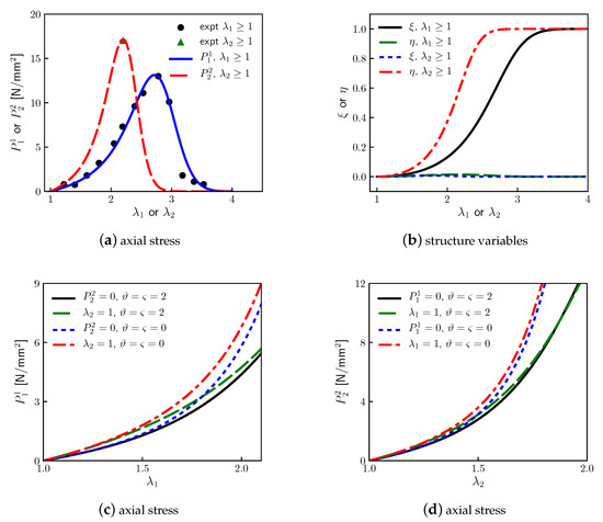
Figure 4. Uniaxial extension and tearing of skin for the imposed axial stretch ${\lambda }_1\ge 1$ or ${\lambda }_2\ge 1$, 2D model: (a) Stress $P_1^1$ or $P_2^2$ (baseline parameters, Table 1) with representative experimental data [74] (see text Section 4.5.1 for the consistent definition of experimental stretch, accounting for pre-stress) for straining perpendicular or parallel to Langer’s lines; (b) normalized internal structure components $\xi$ and $\eta$ (baseline parameters); (c) stress $P_1^1$ for moderate extension ${\lambda }_1\le 2.1$ under uniaxial stress ($P_2^2=0$) or uniaxial strain (${\lambda }_2=1$) conditions for the Finsler model (baseline parameters) and the ideal elastic model ($\vartheta =\varsigma =0$); (d) stress $P_2^2$ for moderate extension ${\lambda }_2\le 2.0$ under uniaxial stress ($P_1^1=0$) or uniaxial strain (${\lambda }_1=1$) conditions for the Finsler model (baseline) and the ideal elastic model ($\vartheta =\varsigma =0$).

Remark 64. 

For loading along ${\mathit{n}}_1$, $\xi \to 1$ and $\eta \to 0$ for ${\lambda }_1\gtrsim 3.5$, meaning most internal structure evolution correlates with degradation in this direction, with small transverse effects of $\eta$. Analogously, loading along ${\mathit{n}}_2$ gives $\eta \to 1$ and $\xi \to 0$ for ${\lambda }_2\gtrsim 3$. The rate of increase of $\eta$ with ${\lambda }_2>1$ is more rapid than the rate of increase of $\xi$ with ${\lambda }_1>1$, since the skin degrades sooner and fails at a lower strain for stretching parallel to Langer’s lines. The present diffuse model is an idealization characteristic of experiments when there is no sharp pre-crack [63,68,72,74,87].

Figure 4c,d shows predictions at modest stretch along ${\mathit{n}}_1$ or ${\mathit{n}}_2$ under uniaxial stress conditions identical to those of Figure 4a, as well as uniaxial strain, whereby ${\lambda }_2=1$ or ${\lambda }_1=1$ is enforced using the scheme in Section 5.5.2, rather than respective of $P_2^2=0$ or $P_1^1=0$. Predictions for the ideal elastic case ($\vartheta =\varsigma =0\Rightarrow \xi =\eta =0$) are shown for comparison. The results are stiffer for the ideal elastic case since degradation commensurate with structure change is omitted. In agreement with other data [70], skin is elastically stiffer in uniaxial strain relative to uniaxial stress. Choosing a higher value of $k_0={\kappa }_0/{\mu }_0>1$ in (176) would further increase this difference if merited.

5.5.2. Biaxial Extension

Now, consider the homogeneous biaxial stress extension in the $X^1$ and $X^2$ directions. From symmetry, $P_2^1=0$, $P_1^2=0$, $F_2^1=0$, $F_1^2=0$, and ${\overline{C}}_{12}={\overline{C}}_{21}=0$. The homogeneous deformation fields are

$$\begin{array}{cc}\hfill {\phi }^1& ={\lambda }_1{X}^1,{\phi }^2={\lambda }_2{X}^2;F_1^1={\lambda }_1,F_2^2={\lambda }_2;\hfill \\ \hfill {\overline{C}}_{11}& ={\left({\lambda }_1\right)}^2,{\overline{C}}_{22}={\left({\lambda }_2\right)}^2;J={\lambda }_1{\lambda }_2.\hfill \end{array}$$

(189)

Stretch ratios are ${\lambda }_1>0$ and ${\lambda }_2>0$; both are constants over $\mathcal{M}$. The mechanical boundary conditions are

$${\phi }^1(X^1=\pm L_0)=\pm {\lambda }_1{L}_0,{\phi }^2(X^2=\pm W_0)=\pm {\lambda }_2{W}_0.$$

(190)

With ${\lambda }_1$ and ${\lambda }_2$ prescribed by (190), equilibrium equations (183) and (184) are solved simultaneously for $\xi$ and $\eta$ as functions of ${\lambda }_1,{\lambda }_2$, giving homogeneous values of fields consistent with (185). Then $P_1^1$ and $P_2^2$ are obtained with (182) for $a=A=1$ and $a=A=2$.

Model predictions for equi-biaxial stretching, ${\lambda }_1={\lambda }_2$, are produced using the baseline material parameters of Table 1, obtained for the 2D theory in Section 5.5.1. In Figure 5a, stresses also include those for the ideal elastic case ($\vartheta =\varsigma =0\Rightarrow \xi =\eta =0$) that are noticeably higher for ${\lambda }_1>1.5$ and increase monotonically with stretch. For the Finsler theory, under this loading protocol (${\lambda }_1={\lambda }_2$), $P_2^2$ increases more rapidly than $P_1^1$, with increasing ${\lambda }_1$, reaching a slightly lower peak value at a significantly lower stretch. Elastic stiffness during the lower-stretch loading is higher in the ${\mathit{n}}_2$ direction due to the preponderance of aligned collagen fibers, but degradation linked to the internal structure evolution is more rapid due to the lower toughness of skin when torn in this direction. The latter phenomena are evident in Figure 5b: $\eta \left({\lambda }_1\right)>\xi \left({\lambda }_1\right)$ for ${\lambda }_1\in [1.1,3.9]$.

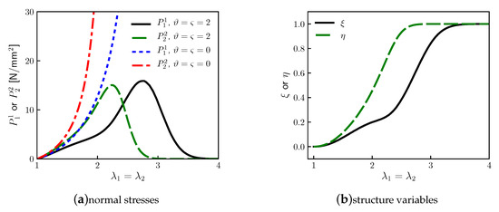
Figure 5. Equi-biaxial extension and tearing of skin, 2D model: (a) stress components from the Finsler model (baseline parameters, $\vartheta =\varsigma =2$) and the ideal elastic model ($\vartheta =\varsigma =0$); (b) normalized internal structure components $\xi$ and $\eta$.

Remark 65. 

Data on failure of skin focus on its uniaxial extension [74,75]. Biaxial data (e.g., [68,70]) do not report stretch magnitudes that are capable of causing tearing, so direct validation does not appear possible. If the skin proves to be stiffer and more damage-tolerant under equi-biaxial stretch, the w of (176) can be modified, so the tangent bulk modulus proportional to $k_0$ increases more strongly with J, and does not degrade so severely with structure evolution.

5.5.3. Stress-Free States

Protocols of Section 5.3.2 now apply. Two boundary value problems are addressed that parallel the 1D analysis of Section 4.5.2. External boundary conditions are set as $\xi =0$ and $\eta =0$, everywhere along $\partial \mathcal{M}$. Stress $P_a^A=0$ prevails everywhere in $\mathcal{M}$, ensuring that the mechanical traction $p_a=P_a^A{N}_A=0$ over $\partial \mathcal{M}$. For the generalized Finsler metric in (172), it is essential to restrict $r>1\Rightarrow {\chi }_1(\xi =0)={\chi }_2(\eta =0)=0$ in (173).

In the first problem, assume that the specimen undergoes a uniaxial stretch along the ${\mathit{n}}_1$ direction (i.e., along $X^1$, perpendicular to Langer’s lines) until localized failure occurs. The skin ruptures completely across the midspan at $X^1=0$, such that $\xi (0,X^2)=1$. In this ruptured state, ${\overline{C}}_{AB}={\delta }_{AB}$ is everywhere on $\mathcal{M}$ for all components, except ${\overline{C}}_{11}$, which can differ from ${\delta }_{AB}$ along the line $X^1=0$. The solution for $\eta (X^1,X^2)$ is $\eta (X^1,X^2)=0$, for which (166) is trivially satisfied. From symmetry, the remaining unknown field $\xi$ depends only on $X=X^1$, and $\xi (-X)=\xi \left(X\right)$. With this partial solution, Equation (165) has a vanishing right side, reducing it to a generally nonlinear, autonomous second-order ODE

$$\begin{array}{c}\hfill {\gamma }_{\xi }\frac{{\mathrm{d}}^2\xi }{\mathrm{d}{X}^2}=\frac{{\gamma }_{\xi }\xi }{l^2}\left(1+k{\xi }^r\right).\end{array}$$

(191)

Dividing by ${\gamma }_{\xi }>0$, (191) is identical to (131) with $N_0=0$, $\lambda ={\xi }^2$, and $\chi ={\chi }_1=k{\xi }^{r-1}$. Solutions (133) and (144) hold verbatim.

The normalized energy per unit area normal to the $X^1$ direction is

$${\overline{\gamma }}_1=\frac{1}{2{{\rm Y}}_0}{\int }_{-L_0}^{L_0}\psi \sqrt{G}\mathrm{d}X=\frac{{\gamma }_{\xi }}{2l}{\int }_{-L_0}^{L_0}\{{\xi }^2+l^2{(\mathrm{d}\xi /\mathrm{d}X)}^2\}\exp \left[(k/r){\xi }^r\right]\mathrm{d}X,$$

(192)

which is identical to (145) when ${\gamma }_{\xi }=1$ and $N_0=0$. Given ${\gamma }_{\xi }=1$, $k=0.2$, $r=2$, and ${{\rm Y}}_0=0.47$ kJ/m${}^2$ (Table 1), the outcomes of the 2D theory here match those of the 1D theory in Figure 3a,b with $N_0=0$ and ${\overline{\gamma }}_1=\overline{\gamma }$. Toughness $2{\overline{\gamma }}_1{{\rm Y}}_0=1.0$ kJ/m${}^2$ is consistent with the experiment [73,99,113].

In the second problem, assume that the specimen is stretched along ${\mathit{n}}_2$ (i.e., along $X^2$, parallel to Langer’s lines). The skin ruptures completely across the midspan at $X^2=0$, with $\eta (X^1,0)=1$. Now, ${\overline{C}}_{AB}={\delta }_{AB}$ is everywhere for all components, except ${\overline{C}}_{22}$, which can differ from ${\delta }_{AB}$ only along $X^2=0$. The solution for $\xi (X^1,X^2)$ is $\xi =0$, for which (165) is trivially obeyed. From symmetry, $\eta$ depends only on $X=X^2$, and $\eta (-X)=\eta \left(X\right)$. The balance law (166) reduces to

$$\begin{array}{c}\hfill {\gamma }_{\eta }\frac{{\mathrm{d}}^2\eta }{\mathrm{d}{X}^2}=\frac{{\gamma }_{\eta }\eta }{l^2}\left(1+m{\eta }^r\right).\end{array}$$

(193)

Dividing by ${\gamma }_{\eta }>0$, (193) matches (131) with $N_0=0$, $\nu ={\eta }^2$, $\chi ={\chi }_2=m{\eta }^{r-1}$, and changes in variables. Solutions (133) and (144) hold. The normalized energy per unit area is

$${\overline{\gamma }}_2=\frac{1}{2{{\rm Y}}_0}{\int }_{-L_0}^{L_0}\psi \sqrt{G}\mathrm{d}X=\frac{{\gamma }_{\eta }}{2l}{\int }_{-L_0}^{L_0}\{{\eta }^2+l^2{(\mathrm{d}\eta /\mathrm{d}X)}^2\}\exp \left[(m/r){\eta }^r\right]\mathrm{d}X$$

(194)

for free surfaces normal to the $X^2$ direction, matching (145) if ${\gamma }_{\eta }=1$ and $N_0=0$. Given ${\gamma }_{\eta }=0.84$, $m=0.3$, $r=2$, and ${{\rm Y}}_0=0.47$ kJ/m${}^2$ (Table 1), profiles of $\eta \left(X\right)$ for this problem are very similar to those of $\xi \left(X\right)$ from the 1D theory in Figure 3a. Energy for $N_0=0$ in Figure 3b transforms as ${\overline{\gamma }}_2\approx {\gamma }_{\eta }\overline{\gamma }$, and $2{\overline{\gamma }}_2{{\rm Y}}_0=0.85$ kJ/m${}^2$ is within experimental ranges of 0.5 to 2.5 kJ/m${}^2$ [73,99,113].

Remark 66. 

Since $2{\overline{\gamma }}_2{{\rm Y}}_0<2{\overline{\gamma }}_1{{\rm Y}}_0$, the model predicts that skin is more brittle in directions parallel to Langer’s lines than in directions perpendicular to Langer’s lines, in concurrence with experiment [74,87]. Collagen fibers are less coiled initially in directions parallel to Langer’s lines [75], giving the skin’s lower compliance and less potential strain accommodation at rupture in those directions.

Remark 67. 

All parameters in Table 1 have clear physical or geometric origins; none are ad hoc. Constant l is the critical fiber-sliding distance or crack-opening displacement for rupture. Ratios $\frac{k}{r}$ and $\frac{m}{r}$ are associated with the remnant strain contributions in orthogonal ${\mathit{n}}_1$ and ${\mathit{n}}_2$ directions along the primary initial fiber directions (e.g., perpendicular and parallel to Langer’s lines). The isotropic shear modulus and bulk modulus for the matrix, consisting of ground substance and elastin, are ${\mu }_0$ and ${\kappa }_0$. Nonlinear elastic constants $a_1$ and $b_1$ control stiffening due to collagen fiber elongation in the ${\mathit{n}}_1$ direction, while $a_2$ and $b_2$ control stiffening due to fiber elongation in the ${\mathit{n}}_2$ direction. The loss of elastic stiffness due to fiber rearrangements and damage processes in matrix, fibers, and their interfaces, in the respective ${\mathit{n}}_1$ and ${\mathit{n}}_2$ directions, is modulated by $\vartheta$ and $\varsigma$. Isotropic surface energy is ${{\rm Y}}_0$, with factors ${\gamma }_{\xi }$ and ${\gamma }_{\eta }$ scaling the fracture toughness in the respective ${\mathit{n}}_1$ and ${\mathit{n}}_2$ directions.

6. Conclusions

A theory of finite-deformation continuum mechanics, rooted in the generalized geometry of Finsler, has been developed and refined. Elements of an internal state vector represent evolving microstructure features and can be interpreted as order parameters. The dependence of the material metric on this internal state affects how distances are measured in the material manifold and how gradients (i.e., covariant derivatives) are resolved. A new application of the theory to anisotropic soft-tissue mechanics has been presented, whereby the internal state is primarily associated with collagen fiber rearrangements and breakages. The material metric contains explicit contributions from sliding or opening modes in different material directions. Solutions to boundary value problems for tensile extension with tearing in different directions agree with experimental data and microscopic observations on skin tissue, providing physical and geometric insight into the effects of the microstructure.

Appendix A.1. Deformation Gradient and Director Gradient

The first of (80) follows from (57), (61), and commutation of $\delta (·)$ and ${\partial }_A(·)$ operators since the variation is performed at fixed $X^A$:

$$\delta F_A^a(\phi \left(X\right),X)=\delta \left({\partial }_A{\phi }^a\left(X\right)\right)={\partial }_A\left(\delta {\phi }^a\left(X\right)\right)={\delta }_A\left(\delta {\phi }^a\left(X\right)\right)={\left(\delta {\phi }^a\left(X\right)\right)}_{|A},$$

(A1)

with $\mathit{F}$ treated as a two-point tensor.

Remark A1. 

The third equality in (A1) follows from $N_A^B(X,D){\overline{\partial }}_B{\phi }^a\left(X\right)=0$. The leftmost and rightmost equalities interpret ${\phi }^a\left(X\right)$ and $\delta {\phi }^a\left(X\right)$, respectively, as point functions rather than vector fields [20,22].

Let $f(X,D)$ denote a generic differentiable function of arguments $\{X^A,D^A\}$ in a coordinate chart on $\mathcal{Z}$. The variation of $f(X,D)$ is defined by the first of the following:

$${\delta f(X,D)=f(X,D)|}_A\delta \left(D^A\right)={\overline{\partial }}_{A}f(X,D)\delta \left(D^A\right),$$

(A2)

where ${(·)|}_A$ is the vertical covariant derivative (e.g., as in (21)). For the choices $V_{BC}^A=0$ and $Y_{BC}^A=0$ of (71), ${f(X,D)|}_A={\overline{\partial }}_{A}f(X,D)$ and the rightmost form is obtained, consistent with prior definitions [54,55]. This is used with (84) to obtain the second of (80):

$$\begin{array}{cc}\hfill \delta D_{|B}^A& =\delta \left({\partial }_B{D}^A\right)-\delta N_B^A+\delta \left(K_{BC}^A\right)D^C+K_{BC}^A\delta \left(D^C\right)\hfill \\ & =[{\partial }_B\delta \left(D^A\right)-N_B^C{\overline{\partial }}_C\delta \left(D^A\right)+K_{BC}^A\delta \left(D^C\right)]-{\overline{\partial }}_C{N}_B^A\delta \left(D^C\right)+{\overline{\partial }}_D{K}_{BC}^A{D}^C\delta \left(D^D\right)\hfill \\ \hfill & ={\left[\delta \left(D^A\right)\right]}_{|B}-({\overline{\partial }}_C{N}_B^A-{\overline{\partial }}_C{K}_{BD}^A{D}^D)\delta \left(D^C\right),\hfill \end{array}$$

(A3)

where it is assumed per (68) that ${\overline{\partial }}_C\delta \left[D^A\left(X\right)\right]={\overline{\partial }}_C\left[\delta \left(D^A\right)\left(X\right)\right]=0$ on $\mathcal{M}$ and $\mathcal{Z}$.

Appendix A.2. Volume Form

Two definitions have been set forth in prior work for the variation of the volume form $d\Omega (X,D)$. The first quoted here sets [54]

$$\begin{array}{cc}\hfill \delta (d\Omega )& =[\delta \sqrt{G}/\sqrt{G}]d\Omega =(ln\sqrt{G}){{|}_A\delta \left(D^A\right)d\Omega =\frac{1}{2}{G}^{BC}{G}_{CB}|}_A\delta \left(D^A\right)d\Omega \hfill \\ & =(C_{AB}^B-Y_{AB}^B)\delta \left(D^A\right)d\Omega =C_{AB}^B\delta \left(D^A\right)d\Omega ,\hfill \end{array}$$

(A4)

where the first equality is a definition and (27) and (A2) is used subsequently.

Remark A2. 

According to (A4), the magnitude of the volume form is varied locally over the n-dimensional base space in (81) with the $\alpha =1$ prior application of the divergence theorem (31) used to procure (87) and (88) from (86) of Section 3.3.3. The choice (A4) was used in the most recent theory [54] and implied in a prior numerical implementation [59].

The second definition quoted here was used in the original theoretical works [55,56]:

$$\begin{array}{cc}\hfill \delta (d\Omega )& =[\delta \sqrt{\mathcal{G}}/\sqrt{\mathcal{G}}]d\Omega =(ln\sqrt{\mathcal{G}}){|}_A\delta \left(D^A\right)d\Omega =(ln\sqrt{G^2}){|}_A\delta \left(D^A\right)d\Omega \hfill \\ & \hfill =G^{BC}{G}_{CB}{|}_A\delta \left(D^A\right)d\Omega =2(C_{AB}^B-Y_{AB}^B)\delta \left(D^A\right)d\Omega =2C_{AB}^B\delta \left(D^A\right)d\Omega .\end{array}$$

(A5)

In the derivation of (A5), the determinant of the Sasaki metric, as defined in (15), has been used along with (27) and (A2).

Remark A3. 

The definition given by the first equality in (A5) is notionally consistent with another earlier theory [49,50,52]. In the present viewpoint with (A5), the magnitude of the volume form is varied locally in a 2n-dimensional total space $\mathcal{Z}$ via (81) with $\alpha =2$ before integrating over the base n-dimensional space $\mathcal{M}$ in (86) of Section 3.3.3.

Remark A4. 

Definition (A4) corresponds to $\alpha =1$ and definition (A5) to $\alpha =2$ in (81). The only ramification in the governing Euler–Lagrange equations involves the scaling of local free energy density by a factor of one or two through $\alpha \psi C_{CA}^A$ in the micro-momentum balance, in either form (88) or (91). Macroscopic momentum is unaffected by the definition of $\delta (d\Omega )$.

Appendix B.1. Macroscopic Momentum

Consideration of residual stress begins with the examination of the balance of linear momentum in the form (90), repeated and reorganized for convenience:

$${\partial }_A{P}_a^A+P_a^B{\gamma }_{AB}^A-P_c^A{\gamma }_{ba}^c{F}_A^b=-\{[{\overline{\partial }}_B{P}_a^A+P_a^A{\overline{\partial }}_B(ln\sqrt{G})]{\partial }_A{D}^B+P_c^A({\gamma }_{ba}^c-{\Gamma }_{ba}^c)F_A^b\}.$$

(A6)

Remark A5. 

Terms on the left side of (A6) are standard for nonlinear elasticity theory [22]. If the free energy $\psi$ does not depend on $D^A$ or $D_{|B}^A$, then the stress $P_a^A=\partial \psi /\partial F_A^a$ is also conventional, presuming $\psi$ is in the undeformed state $C_{AB}=G_{AB}\Rightarrow P_a^A=0$. In that case, when the right side of (A6) vanishes, the body manifold $\mathcal{M}$ should not contain residual stresses when $F_A^a={\partial }_A{\phi }^a$ for regular motions ${\phi }^a\left(X\right)$ (e.g., in the absence of topological changes).

Remark A6. 

Departures from classical nonlinear elasticity arise when (i) $\psi$ has dependencies on $D^A$ or $D_{|B}^A$, (ii) when $P_a^A$ or G depends on $D^A$ along with the heterogeneous state field ${\partial }_A{D}^B\ne 0$, or (iii) when a different connection than the Levi–Civita connection is used for ${\Gamma }_{ba}^c$ (i.e., ${\Gamma }_{ba}^c\ne {\gamma }_{ba}^c$ due to the d dependence of the spatial metric $g_{ab}$). Each of these departures could potentially induce stresses $P_a^A\ne 0$ in a simply connected body externally unloaded via $p_a=P_a^A{N}_A=0$ all along its oriented boundary $\partial \mathcal{M}$ (i.e., residual stresses).

Analysis of a particular version of the general theory offers more insight. First, assume in (74) that ${\widehat{g}}_b^a\to {\delta }_b^a$, such that $g_{ab}(x,d)\to g_{ab}\left(x\right)={\overline{g}}_{ab}\left(x\right)$; the spatial metric tensor $\mathit{g}$ is Riemannian rather than Finslerian. Then, ${\gamma }_{bc}^a={\Gamma }_{bc}^a$. Now, use the osculating Riemannian interpretation of the Finslerian material metric $\mathit{G}$ offered by Corollary 1 via (68):

$${\tilde{G}}_{AB}\left(X\right)=G_{AB}(X,D\left(X\right)),\tilde{G}\left(X\right)=det\left({\tilde{G}}_{AB}\left(X\right)\right),$$

(A7)

$${\tilde{\gamma }}_{BA}^A={\partial }_B(ln\sqrt{\tilde{G}})={\partial }_B(ln\sqrt{G})+{\overline{\partial }}_A(ln\sqrt{G}){\partial }_B{D}^A={\gamma }_{BA}^A+{\overline{\partial }}_A(ln\sqrt{G}){\partial }_B{D}^A,$$

(A8)

$${\tilde{P}}_a^A\left(X\right)=P_a^A(X,D\left(X\right)),{\partial }_B{\tilde{P}}_a^A={\partial }_B{P}_a^A+{\overline{\partial }}_C{P}_a^A{\partial }_B{D}^C.$$

(A9)

Substituting (A8) and (A9) into (A6) gives, with ${\gamma }_{ba}^c={\Gamma }_{ba}^c$,

$${\partial }_A{\tilde{P}}_a^A+{\tilde{P}}_a^B{\tilde{\gamma }}_{AB}^A-{\tilde{P}}_c^A{\gamma }_{ba}^c{F}_A^b=0.$$

(A10)

Remark A7. 

Expression (A10) conforms to the standard form for static equilibrium in classical continuum mechanics, but stress, denoted as ${\tilde{P}}_a^A$, and the connection, represented by ${\tilde{\gamma }}_{BC}^A$, both implicitly depend on the internal state $D^A$, and the former might also depend on its gradient $D_{|B}^A$, especially if it appears in appearing in $\psi$. Coefficients ${\tilde{\gamma }}_{BC}^A$ are those of the Levi–Civita connection of ${\tilde{G}}_{AB}$ via (36).

Now neglecting the dependence on the internal state gradient in the energy density, requiring D dependence to arise only through $G_{AB}$, and assuming the body is homogeneous (with a mild abuse of notation):

$$\begin{array}{cc}\hfill \psi & =\psi (F_A^a,D^A)=\psi (F_A^a,G_{AB}(X,D))\hfill \\ & =\tilde{\psi }(F_A^a,{\tilde{G}}_{AB}\left(X\right))=\tilde{\psi }(C_{AB}(F_A^a,g_{ab}),{\tilde{G}}_{AB}\left(X\right)).\hfill \end{array}$$

(A11)

Recall from (66) that $C_{AB}=F_A^a{g}_{ab}{F}_B^b$. As a simple example, consider the case where $n=dim\mathcal{M}$,

$$\begin{array}{cc}\hfill \tilde{\psi }& =\frac{{\mu }_0}{2}(C_{AB}{\tilde{G}}^{AB}-n)\hfill \\ & \Rightarrow {\tilde{P}}_a^A=\frac{\partial \tilde{\psi }}{\partial F_a^A}={\mu }_0{g}_{ab}{\tilde{G}}^{AB}{F}_A^b,\frac{\partial \tilde{\psi }}{\partial {\tilde{G}}^{AB}}=-\frac{{\mu }_0}{2}{\tilde{G}}^{AC}{\tilde{G}}^{BD}{C}_{CD},\hfill \end{array}$$

(A12)

and where ${\mu }_0>0$ is a constant (e.g., an elastic shear modulus). Now, assume that the spatial manifold $\mathfrak{m}$ is Euclidean [27,30], such that the Riemann–Christoffel curvature tensor from ${\gamma }_{bc}^a$ (and, thus, derived from $g_{ab}$) vanishes identically.

Remark A8. 

In this case, (A10), the last of (A11), and the example (A12) are consistent with the geometric theory of the growth mechanics of Yavari [30] in the quasi-static setting. Incompressibility can be addressed by appending linear momentum to include contributions from an indeterminant pressure to be determined by boundary conditions under the isochoric constraint $J=1$ [22]. Otherwise, $\tilde{\psi }$ can be augmented with term(s) to ensure $C_B^A\to {\delta }_B^A\Rightarrow {\tilde{P}}_a^A=0$ (e.g., (138) for $n=1$).

The Riemann–Christoffel curvature tensor from ${\tilde{\gamma }}_{BC}^A$ (and, thus, ${\tilde{G}}_{AB}$) need not vanish in general:

$${\tilde{\mathcal{R}}}_{BCD}^A={\partial }_B{\tilde{\gamma }}_{CD}^A-{\partial }_C{\tilde{\gamma }}_{BD}^A+{\tilde{\gamma }}_{BE}^A{\tilde{\gamma }}_{CD}^E-{\tilde{\gamma }}_{CE}^A{\tilde{\gamma }}_{BD}^E.$$

(A13)

Remark A9. 

In Riemannian geometry, ${\tilde{\gamma }}_{BC}^A$ are symmetric, differentiable, and obey (36); (A13) has $\frac{1}{12}{n}^2(n^2-1)$ independent components [31]. For $n=3$, ${\tilde{\mathcal{R}}}_{BCD}^A$ contains six independent components, determined completely by the metric and the Ricci curvature ${\tilde{\mathcal{R}}}_{ABC}^A$ [30,98]. For $n=2$, ${\tilde{\mathcal{R}}}_{BCD}^A$ contains only one independent component, determined completely by the scalar curvature $\tilde{\kappa }=\frac{1}{2}{\mathcal{R}}_{AB}{\tilde{G}}^{AB}$. For $n=1$, ${\tilde{\mathcal{R}}}_{BCD}^A$ always vanishes (i.e., a 1D manifold is always flat in this sense).

When ${\tilde{\mathcal{R}}}_{BCD}^A$ is nonzero over a region of $\mathcal{M}$, then no compatible deformation ${\tilde{F}}_a^A\left(X\right)$ exists that can push forward ${\tilde{G}}_{AB}$ to match the Euclidean metric $g_{ab}\left(\varphi \left(X\right)\right)$, which would render the corresponding regions of $\mathcal{M}$ and $\mathfrak{m}$ isometric. In other words, the push-forward $g_{ab}={\tilde{F}}_a^A{\tilde{G}}_{AB}{\tilde{F}}_b^B$ where ${\tilde{F}}_a^A={\partial }_a{\zeta }^A$ does not exist, ${\zeta }^A$ being (nonexistent) Euclidean coordinates on $\mathcal{M}$. In such cases, $\mathcal{M}$ would always have to be deformed (e.g., strained) to achieve its spatial representation $\mathfrak{m}$ since no isometry exists between the two configurations.

Remark A10. 

If an intrinsically curved body manifold in the reference state $\mathcal{M}$ is stress-free, per the constitutive prescription (e.g., (A12) or any other standard elasticity model), then the intrinsically flat body in the current state $\mathfrak{m}$ would be necessarily strained and stressed, even if external traction $p_a$ vanishes along its boundary. Thus, this particular rendition of the generalized Finsler theory supplies residual stress from a non-Euclidean material metric tensor ${\tilde{G}}_{AB}$ in a manner matching other works that use Riemannian geometry [27,30].

In the full version of the generalized Finsler theory [54,55], as discussed following (A6), residual stresses could emerge from additional sources to those discussed under the foregoing assumptions of a Euclidean spatial metric, a conventional hyperelastic energy potential, and an osculating Riemannian material metric with non-vanishing curvature. Several different curvature forms can be constructed from the various connections and derivatives of Finsler geometry and its generalizations [3,5]. Further analysis, beyond the present scope, is needed to relate these geometric objects to physics in the continuum mechanical setting, including residual stresses.

Remark A11. 

The deformation gradient $F_A^a$ could be decomposed into a product of two mappings [62]: $F_A^a\left(X\right)={\partial }_A{\phi }^a\left(X\right)={\left(F^E\right)}_{\alpha }^a\left(X\right){\left(F^D\right)}_A^{\alpha }\left(D\left(X\right)\right)$. In this case, the strain energy potential is written to emphasize the elastic deformation ${\mathit{F}}^E$, with the state-dependent deformation ${\mathit{F}}^D$ explicitly accounting for inelastic deformation mechanisms, including growth [29,107]. In this setting, residual stresses can arise if ${\left({\mathit{F}}^E\right)}^{-1}$ and, thus, ${\mathit{F}}^D$ do not fulfill certain integrability conditions; neither the two-point tensor ${\left({\mathit{F}}^E\right)}^{-1}$ nor ${\mathit{F}}^D$ is always integrable to a vector field [98].

Appendix B.2. Micro-Momentum and Growth

Now, consider the internal state-space equilibrium equation, (91) first, under the aforementioned assumptions used to derive (A10). Furthermore, let $N_B^A=N_B^A\left(X\right)$$K_{BC}^A={\gamma }_{BC}^A\left(X\right)$, and $\alpha =1$. Then, with these assumptions, in the osculating Riemannian interpretation of Corollary 1, (91) is

$$\begin{array}{c}\hfill {\partial }_A{\tilde{Z}}_C^A+{\tilde{Z}}_C^B{\tilde{\gamma }}_{AB}^A-{\tilde{Z}}_B^A{\gamma }_{AC}^B-Q_C=\psi {\overline{\partial }}_C(ln\sqrt{G})-R_C,\end{array}$$

(A14)

$${\tilde{Z}}_B^A\left(X\right)=Z_B^A(X,D\left(X\right))=\frac{\partial \psi }{\partial D_{|A}^B}(X,D\left(X\right)),Q_A(X,D\left(X\right))=\frac{\partial \psi }{\partial D^A}(X,D\left(X\right)),$$

(A15)

where (A15) follows from (85). Use the energy density $\psi$ of (A11), so ${\tilde{Z}}_B^A=0$ identically. Choose the volumetric source term $R_C=\psi {\overline{\partial }}_C(ln\sqrt{G})$, which here represents the local change in referential volumetric energy density due to growth effects on the local volume form $d\Omega (X,D)$, since now, per (A4) of Appendix A, $\psi \delta (d\Omega )=\psi \left[{\overline{\partial }}_C(ln\sqrt{G})\delta \left(D^C\right)\right]d\Omega =R_C\delta \left(D^C\right)d\Omega$.

Remark A12. 

Physical justification exists in the context of growth mechanics for biological systems: $R_C$ can account for the effect on energy density from changes in mass due to tissue growth [30,107]. Thus, (A14) further reduces to, with (A11), to a form very similar to the equilibrium case of Yavari [30] (e.g., matching Equation (2.73) of ref. [30] with the vanishing time derivative, if, here, ${\overline{\partial }}_A{G}_{BC}$ is arbitrary):

$$Q_A=\frac{\partial \psi }{\partial D^A}=\frac{\partial \psi }{\partial G_{BC}}\frac{\partial G_{BC}}{\partial D^A}=\frac{\partial \tilde{\psi }}{\partial {\tilde{G}}_{BC}}\frac{\partial G_{BC}}{\partial D^A}=0.$$

(A16)

To see how internal state components $\left\{D^A\right\}$ can represent growth, consider $n=2$ (i.e., 2D $\mathcal{M}$, such as a biological membrane), by which, $\left\{D^A\right\}\to (D^1,D^2)=(l_1{\xi }^1,l_2{\xi }^2)$, where $l_{1,2}>0$ are normalization constants that render the ${\xi }^A$ dimensionless. Choose a polar (i.e., cylindrical $\left\{X^A\right\}\to (R,\Theta$)) coordinate system on a region of $\mathcal{M}$ with (73) applying, such that $\overline{\mathit{G}}=\mathrm{diag}(1,R^2)$. Assume a generalized Finslerian contribution $\widehat{\mathit{G}}=\mathrm{diag}(\exp \left(h_1\left({\xi }^1\right)\right),\exp \left(h_2\left({\xi }^2\right)\right)$, where $h_1\left(D\left(X\right)\right)=h_1(D^1(R,\Theta )/l_1)$ and $h_2\left(D\left(X\right)\right)=h_2(D^2(R,\Theta )/l_2)$ are differentiable functions of their arguments. In matrix form, in this example of anisotropic growth, the second of (73) becomes

$$\left[G_{AB}\right]=\left[\begin{array}{cc}{G}_{RR}& 0\\ 0& G_{\Theta \Theta }\end{array}\right]=\left[{\widehat{G}}_A^C\right]\left[{\overline{G}}_{CB}\right]=\left[\begin{array}{cc}\exp \left(h_1\left({\xi }^1\right)\right)& 0\\ 0& R^2\exp \left(h_2\left({\xi }^2\right)\right)\end{array}\right].$$

(A17)

A more specific case is now studied. Let $\chi \left(R\right)$ denote a scalar radial growth function. Then set

$$\xi ={\xi }^1=\frac{D^1}{l_1}=\frac{D^2}{l_2}={\xi }^2,\xi =\xi \left(R\right);h=h_1=-h_2=2\chi ,h=h\left(\xi \left(R\right)\right)=2\chi \left(R\right).$$

(A18)

This yields the metric ${\tilde{G}}_{AB}\left(X\right)$ as per Yavari (ref. [30], Equation (2.101)), which corresponds to anisotropic annular growth:

$$\begin{array}{cc}\hfill \left[G_{AB}(R,\xi )\right]& =\left[\begin{array}{cc}\exp \left(h\right(\xi \left(R\right)\left)\right)& 0\\ 0& R^2\exp (-h\left(\xi \left(R\right)\right))\end{array}\right]\hfill \\ \hfill \Rightarrow \left[{\tilde{G}}_{AB}\left(R\right)\right]& =\left[\begin{array}{cc}\exp \left(2\chi \right(R\left)\right)& 0\\ 0& R^2\exp (-2\chi \left(R\right))\end{array}\right].\hfill \end{array}$$

(A19)

Remark A13. 

In the special case given by (A19), internal state changes preserve volume via $det\left(G_{AB}(X,D)\right)=R^2$ being independent of $\chi$, $\xi$, and D, so $C_{AB}^B=0$.

Now, the energy potential (A12) is applied, so that, for equilibrium of the internal state, (A16) transitions to the following, defining $\dot{h}\left(\xi \right)=\mathrm{d}h\left(\xi \right)/\mathrm{d}\xi$,

$$\begin{array}{cc}\hfill Q_A& =-\frac{{\mu }_0}{2}{\tilde{G}}^{BD}{\tilde{G}}^{CE}{C}_{DE}{\overline{\partial }}_A{G}_{BC}=0\hfill \\ & \Rightarrow \left\{\begin{array}{c}2l_1{Q}_1(\xi ,R)=-{\mu }_0\exp (-h\left(\xi \right))C_{RR}\dot{h}\left(\xi \right)=0,\hfill \\ 2l_2{Q}_2(\xi ,R)={\mu }_0{R}^{-2}\exp \left(h\left(\xi \right)\right)C_{\Theta \Theta }\dot{h}\left(\xi \right)=0.\hfill \end{array}\right.\hfill \end{array}$$

(A20)

Thus, the equilibrium of the internal state is only ensured for this particular strain energy function and material metric when $\dot{h}=0$. A sample function with three equilibrium states at $\xi =0,\frac{1}{2},1$ is the double-well:

$$h={\xi }^2{(1-\xi )}^2,\dot{h}=2\xi (1-\xi )(1-2\xi ).$$

(A21)

Now, the Levi–Civita connection and curvature for the metric $\tilde{\mathit{G}}$ in (A19) are revisited. Denote $h^{\prime }\left(\xi \left(R\right)\right)=[\mathrm{d}h\left(\xi \left(R\right)\right)/\mathrm{d}\xi ][\mathrm{d}\xi \left(R\right)/\mathrm{d}R]=\dot{h}\left(\xi \right){\xi }^{\prime }\left(R\right)$. From (36), ${\tilde{\gamma }}_{BC}^A$ has non-vanishing components

$${\tilde{\gamma }}_{RR}^R=\frac{h^{\prime }}{2},{\tilde{\gamma }}_{\Theta \Theta }^R=\exp (-2h)\left(\frac{R^2{h}^{\prime }}{2}-R\right),{\tilde{\gamma }}_{R\Theta }^{\Theta }={\tilde{\gamma }}_{\Theta R}^{\Theta }=\frac{1}{R}-\frac{h^{\prime }}{2}.$$

(A22)

Recalling that $\tilde{\kappa }$ is the scalar curvature, the non-vanishing covariant components of ${\tilde{\mathcal{R}}}_{BCDE}={\tilde{\mathcal{R}}}_{BCD}^A{\tilde{G}}_{AE}$ are from (A13),

$$\begin{array}{cc}\hfill & {\tilde{\mathcal{R}}}_{R\Theta R\Theta }={\tilde{\mathcal{R}}}_{\Theta R\Theta R}=-{\tilde{\mathcal{R}}}_{R\Theta \Theta R}=-{\tilde{\mathcal{R}}}_{\Theta RR\Theta }=-R^2\tilde{\kappa }\hfill \\ & =-[{\partial }_R{\tilde{\gamma }}_{\Theta \Theta }^R+{\tilde{\gamma }}_{\Theta \Theta }^R({\tilde{\gamma }}_{RR}^R-{\tilde{\gamma }}_{R\Theta }^{\Theta })]{\tilde{G}}_{RR}\hfill \\ & =-\frac{\mathrm{d}}{\mathrm{d}R}\left[\exp (-2h)\left(\frac{R^2{h}^{\prime }}{2}-R\right)\right]\exp \left(h\right)+\left(\frac{R^2{h}^{\prime }}{2}-R\right)\left(\frac{1}{R}-h^{\prime }\right)\exp (-h)\hfill \\ & =-\frac{R}{2}\exp (-h)\left[R\{h^{″}-{\left(h^{\prime }\right)}^2\}+4h^{\prime }\right]\hfill \\ & =-\frac{R}{2}\exp (-h)\left[R\left(\frac{{\mathrm{d}}^2\xi }{\mathrm{d}{R}^2}+\frac{\mathrm{d}\xi }{\mathrm{d}R}\frac{\mathrm{d}}{\mathrm{d}R}\right)\frac{\mathrm{d}h}{\mathrm{d}\xi }-R{\left(\frac{\mathrm{d}h}{\mathrm{d}\xi }\frac{\mathrm{d}\xi }{\mathrm{d}R}\right)}^2+4\frac{\mathrm{d}h}{\mathrm{d}\xi }\frac{\mathrm{d}\xi }{\mathrm{d}R}\right].\hfill \end{array}$$

(A23)

The annular material manifold $\{\mathcal{M}:R\in [R_0,R_1],\Theta \in [0,{\Theta }_1]\}$, $R_1>R_0>0$, ${\Theta }_1<2\pi$ is considered. Since $R>0$ and for bounded h, the local flatness condition from (A23) is

$$R\{h^{″}-{\left(h^{\prime }\right)}^2\}+4h^{\prime }=0\leftrightarrow R\left(\frac{{\mathrm{d}}^2\xi }{\mathrm{d}{R}^2}+\frac{\mathrm{d}\xi }{\mathrm{d}R}\frac{\mathrm{d}}{\mathrm{d}R}\right)\frac{\mathrm{d}h}{\mathrm{d}\xi }-R{\left(\frac{\mathrm{d}h}{\mathrm{d}\xi }\frac{\mathrm{d}\xi }{\mathrm{d}R}\right)}^2+4\frac{\mathrm{d}h}{\mathrm{d}\xi }\frac{\mathrm{d}\xi }{\mathrm{d}R}=0.$$

(A24)

Remark A14. 

The first of (A24) is a second-order nonlinear ODE detailing the radial distribution of the generic function $h=h\left(R\right)$. The second is a second-order nonlinear ODE for $\xi =\xi \left(R\right)$, which could be solved if the intermediate functional form $h\left(\xi \right)$ is known a priori (e.g., (A21)). Trivial solutions are $h\left(R\right)=\mathit{constant}$ and $\xi \left(R\right)=\mathit{constant}$. General non-trivial analytical solutions are not obvious. Given the boundary conditions, determining the particular non-trivial solutions for flatness, should they exist, appears to require numerical methods.

References

- Finsler, P. Uber Kurven und Flachen in Allgemeiner Raumen. Ph.D. Thesis, University of Göttingen, Gottingen, Germany, 1918. [Google Scholar]
- Rund, H. The Differential Geometry of Finsler Spaces; Springer: Berlin, Germany, 1959. [Google Scholar]
- Bao, D.; Chern, S.S.; Shen, Z. An Introduction to Riemann-Finsler Geometry; Springer: New York, NY, USA, 2000. [Google Scholar]
- Eringen, A. Tensor Analysis. In Continuum Physics; Eringen, A., Ed.; Academic Press: New York, NY, USA, 1971; Volume I, pp. 1–155. [Google Scholar]
- Bejancu, A. Finsler Geometry and Applications; Ellis Horwood: New York, NY, USA, 1990. [Google Scholar]
- Miron, R. Metrical Finsler structures and metrical Finsler connections. J. Math. Kyoto Univ. 1983, 23, 219–224. [Google Scholar] [CrossRef]
- Watanabe, S.; Ikeda, S.; Ikeda, F. On a metrical Finsler connection of a generalized Finsler metric gij=e2σ(x,y)γij(x). Tensor New Ser. 1983, 39, 97–102. [Google Scholar]
- Matsumoto, M. Foundations of Finsler Geometry and Special Finsler Spaces; Kaiseisha Press: Shigaken, Japan, 1986. [Google Scholar]
- Bejancu, A.; Farran, H. Geometry of Pseudo-Finsler Submanifolds; Kluwer: Dordrecht, The Netherlands, 2000. [Google Scholar]
- Minguzzi, E. The connections of pseudo-Finsler spaces. Int. J. Geom. Methods Mod. Phys. 2014, 11, 1460025. [Google Scholar] [CrossRef]
- Antonelli, P.; Ingarden, R.; Matsumoto, M. The Theory of Sprays and Finsler Spaces with Applications in Physics and Biology; Kluwer: Dordrecht, The Netherlands, 1993. [Google Scholar]
- Vacaru, S.; Stavrinos, P.; Gaburov, E.; Gonţa, D. Clifford and Riemann-Finsler Structures in Geometric Mechanics and Gravity; Geometry Balkan Press: Bucharest, Romania, 2005. [Google Scholar]
- Brandt, H. Differential geometry of spacetime tangent bundle. Int. J. Theor. Phys. 1992, 31, 575–580. [Google Scholar] [CrossRef]
- Voicu, N. New Considerations on Einstein Equations in Pseudo-Finsler Spaces. In Mathematics and Astronomy A Joint Long Journey: Proceedings of the International Conference, Madrid, Spain, 23–27 November 2009; AIP Publishing: Long Island, NY, USA, 2009; Volume 1283, pp. 249–257. [Google Scholar]
- Balan, V.; Bogoslovsky, G.; Kokarev, S.; Pavlov, D.; Siparov, S.; Voicu, N. Geometrical models of the locally anisotropic space-time. arXiv 2011, arXiv:1111.4346. [Google Scholar] [CrossRef]
- Ma, T.; Matveev, V.; Pavlyukevich, I. Geodesic random walks, diffusion processes and Brownian motion on Finsler manifolds. J. Geom. Anal. 2021, 31, 12446–12484. [Google Scholar] [CrossRef]
- Hohmann, M.; Pfeifer, C.; Voicu, N. Mathematical foundations for field theories on Finsler spacetimes. J. Math. Phys. 2022, 63, 032503. [Google Scholar] [CrossRef]
- Popov, N.; Matveev, I. Six-Dimensional Manifold with Symmetric Signature in a Unified Theory of Gravity and Electromagnetism. Symmetry 2022, 14, 1163. [Google Scholar] [CrossRef]
- Abbondandolo, A.; Benedetti, G.; Polterovich, L. Lorentz-Finsler metrics on symplectic and contact transformation groups. arXiv 2022, arXiv:2210.02387. [Google Scholar]
- Truesdell, C.; Toupin, R. The Classical Field Theories. In Handbuch der Physik; Flugge, S., Ed.; Springer: Berlin, Germany, 1960; Volume III/1, pp. 226–793. [Google Scholar]
- Kro¨ner, E. Allgemeine kontinuumstheorie der versetzungen und eigenspannungen. Arch. Ration. Mech. Anal. 1960, 4, 273–334. [Google Scholar] [CrossRef]
- Marsden, J.; Hughes, T. Mathematical Foundations of Elasticity; Prentice-Hall: Englewood Cliffs, NJ, USA, 1983. [Google Scholar]
- Toupin, R.; Rivlin, R. Dimensional changes in crystals caused by dislocations. J. Math. Phys. 1960, 1, 8–15. [Google Scholar] [CrossRef]
- Yavari, A.; Goriely, A. Riemann-Cartan geometry of nonlinear dislocation mechanics. Arch. Ration. Mech. Anal. 2012, 205, 59–118. [Google Scholar] [CrossRef]
- Clayton, J. Defects in nonlinear elastic crystals: Differential geometry, finite kinematics, and second-order analytical solutions. Zeitschrift für Angewandte Mathematik und Mechanik (ZAMM) 2015, 95, 476–510. [Google Scholar] [CrossRef]
- Stojanovitch, R. On the stress relation in non-linear thermoelasticity. Int. J. Non-Linear Mech. 1969, 4, 217–233. [Google Scholar] [CrossRef]
- Ozakin, A.; Yavari, A. A geometric theory of thermal stresses. J. Math. Phys. 2010, 51. [Google Scholar] [CrossRef]
- Takamizawa, K. Stress-Free Configuration of a Thick-Walled Cylindrical Model of the Artery: An Application of Riemann Geometry to the Biomechanics of Soft Tissues. J. Appl. Mech. 1991, 58, 840–842. [Google Scholar] [CrossRef]
- Rodriguez, E.; Hoger, A.; McCulloch, A. Stress-dependent finite growth in soft elastic tissues. J. Biomech. 1994, 27, 455–467. [Google Scholar] [CrossRef]
- Yavari, A. A geometric theory of growth mechanics. J. Nonlinear Sci. 2010, 20, 781–830. [Google Scholar] [CrossRef]
- Schouten, J. Ricci Calculus; Springer: Berlin, Germany, 1954. [Google Scholar]
- Clayton, J. On anholonomic deformation, geometry, and differentiation. Math. Mech. Solids 2012, 17, 702–735. [Google Scholar] [CrossRef]
- Clayton, J. Nonlinear Mechanics of Crystals; Springer: Dordrecht, The Netherlands, 2011. [Google Scholar]
- Steinmann, P. Geometrical Foundations of Continuum Mechanics; Springer: Berlin, Germany, 2015. [Google Scholar]
- Hushmandi, A.; Rezaii, M. On the curvature of warped product Finsler spaces and the Laplacian of the Sasaki-Finsler metrics. J. Geom. Phys. 2012, 62, 2077–2098. [Google Scholar] [CrossRef]
- Watanabe, S.; Ikeda, F. On metrical Finsler connections of a metrical Finsler structure. Tensor New Ser. 1982, 39, 37–41. [Google Scholar]
- Rund, H. A divergence theorem for Finsler metrics. Monatshefte Math. 1975, 79, 233–252. [Google Scholar] [CrossRef]
- Toupin, R. Theories of elasticity with couple stress. Arch. Ration. Mech. Anal. 1964, 17, 85–112. [Google Scholar] [CrossRef]
- Mindlin, R. Microstructure in linear elasticity. Arch. Ration. Mech. Anal. 1964, 16, 51–78. [Google Scholar] [CrossRef]
- Eringen, A. Mechanics of micromorphic continua. In Mechanics of Generalized Continua; Kro¨ner, E., Ed.; Springer: Berlin, Germany, 1968; pp. 18–35. [Google Scholar]
- Regueiro, R. On finite strain micromorphic elastoplasticity. Int. J. Solids Struct. 2010, 47, 786–800. [Google Scholar] [CrossRef][Green Version]
- Eremeyev, V.; Lebedev, L.; Altenbach, H. Foundations of Micropolar Mechanics; Springer: Heidelberg, Germany, 2013. [Google Scholar]
- Eremeyev, V.; Konopińska-Zmyslowska, V. On dynamic extension of a local material symmetry group for micropolar media. Symmetry 2020, 12, 1632. [Google Scholar] [CrossRef]
- Amari, S. A theory of deformations and stresses of ferromagnetic substances by Finsler geometry. In RAAG Memoirs; Kondo, K., Ed.; Gakujutsu Bunken Fukyu-Kai: Tokyo, Japan, 1962; Volume 3, pp. 257–278. [Google Scholar]
- Ikeda, S. A physico-geometrical consideration on the theory of directors in the continuum mechanics of oriented media. Tensor New Ser. 1973, 27, 361–368. [Google Scholar]
- Ikeda, S. On the conservation laws in the theory of fields in Finsler spaces. J. Math. Phys. 1981, 22, 1211–1214. [Google Scholar] [CrossRef]
- Ikeda, S. On the theory of fields in Finsler spaces. J. Math. Phys. 1981, 22, 1215–1218. [Google Scholar] [CrossRef]
- Ikeda, S. On the covariant differential of spin direction in the Finslerian deformation theory of ferromagnetic substances. J. Math. Phys. 1981, 22, 2831–2834. [Google Scholar] [CrossRef]
- Saczuk, J. On the role of the Finsler geometry in the theory of elasto-plasticity. Rep. Math. Phys. 1997, 39, 1–17. [Google Scholar] [CrossRef]
- Stumpf, H.; Saczuk, J. A generalized model of oriented continuum with defects. Zeitschrift für Angewandte Mathematik und Mechanik (ZAMM) 2000, 80, 147–169. [Google Scholar] [CrossRef]
- Stumpf, H.; Saczuk, J. On nonlocal gradient model of inelastic heterogeneous media. J. Theor. Appl. Mech. 2002, 40, 205–234. [Google Scholar]
- Saczuk, J. Finslerian Foundations of Solid Mechanics; Polskiej Akademii Nauk: Gdansk, Poland, 1996. [Google Scholar]
- Yajima, T.; Nagahama, H. Connection structures of topological singularity in micromechanics from a viewpoint of generalized Finsler space. Ann. Phys. 2020, 532, 2000306. [Google Scholar] [CrossRef]
- Clayton, J. Finsler differential geometry in continuum mechanics: Fundamental concepts, history, and renewed application to ferromagnetic solids. Math. Mech. Solids 2022, 27, 910–949. [Google Scholar] [CrossRef]
- Clayton, J. Finsler geometry of nonlinear elastic solids with internal structure. J. Geom. Phys. 2017, 112, 118–146. [Google Scholar] [CrossRef]
- Clayton, J. Finsler-Geometric Continuum Mechanics; Technical Report ARL-TR-7694; DEVCOM Army Research Laboratory: Aberdeen Proving Ground, Aberdeen, MD, USA, 2016. [Google Scholar]
- Clayton, J. Generalized pseudo-Finsler geometry applied to the nonlinear mechanics of torsion of crystalline solids. Int. J. Geom. Methods Mod. Phys. 2018, 15, 1850113. [Google Scholar] [CrossRef]
- Clayton, J. Finsler-geometric continuum dynamics and shock compression. Int. J. Fract. 2017, 208, 53–78. [Google Scholar] [CrossRef]
- Clayton, J.; Knap, J. Continuum modeling of twinning, amorphization, and fracture: Theory and numerical simulations. Contin. Mech. Thermodyn. 2018, 30, 421–455. [Google Scholar] [CrossRef]
- Maugin, G.; Eringen, A. Deformable magnetically saturated media. I. Field equations. J. Math. Phys. 1972, 13, 143–155. [Google Scholar] [CrossRef]
- Maugin, G.; Eringen, A. Deformable magnetically saturated media. II. Constitutive theory. J. Math. Phys. 1972, 13, 1334–1347. [Google Scholar] [CrossRef]
- Clayton, J. Generalized Finsler geometric continuum physics with applications in fracture and phase transformations. Zeitschrift fur Angewandte Mathematik und Physik (ZAMP) 2017, 68, 9. [Google Scholar] [CrossRef]
- Mitsuhashi, K.; Ghosh, S.; Koibuchi, H. Mathematical modeling and simulations for large-strain J-shaped diagrams of soft biological materials. Polymers 2018, 10, 715. [Google Scholar] [CrossRef] [PubMed]
- Takano, Y.; Koibuchi, H. J-shaped stress-strain diagram of collagen fibers: Frame tension of triangulated surfaces with fixed boundaries. Phys. Rev. E 2017, 95, 042411. [Google Scholar] [CrossRef] [PubMed]
- Koibuchi, H.; Sekino, H. Monte Carlo studies of a Finsler geometric surface model. Phys. A 2014, 393, 37–50. [Google Scholar] [CrossRef]
- Koibuchi, H.; Shobukhov, A. Internal phase transition induced by external forces in Finsler geometric model for membranes. Int. J. Mod. Phys. C 2016, 27, 1650042. [Google Scholar] [CrossRef]
- Koibuchi, H.; Bernard, C.; Chenal, J.M.; Diguet, G.; Sebald, G.; Cavaille, J.Y.; Takagi, T.; Chazeau, L. Monte Carlo study of rubber elasticity on the basis of Finsler geometry modeling. Symmetry 2019, 11, 1124. [Google Scholar] [CrossRef]
- Fung, Y.C. Biomechanics: Mechanical Properties of Living Tissues, 2nd ed.; Springer: New York, NY, USA, 1993. [Google Scholar]
- Cowin, S.; Doty, S. Tissue Mechanics; Springer: New York, NY, USA, 2007. [Google Scholar]
- Lanir, Y.; Fung, Y. Two-dimensional mechanical properties of rabbit skin—II. Experimental results. J. Biomech. 1974, 7, 171–182. [Google Scholar] [CrossRef]
- Annaidh, A.; Bruyère, K.; Destrade, M.; Gilchrist, M.; Maurini, C.; Otténio, M.; Saccomandi, G. Automated estimation of collagen fibre dispersion in the dermis and its contribution to the anisotropic behaviour of skin. Ann. Biomed. Eng. 2012, 40, 1666–1678. [Google Scholar] [CrossRef]
- Munoz, M.; Bea, J.; Rodríguez, J.; Ochoa, I.; Grasa, J.; del Palomar, A.; Zaragoza, P.; Osta, R.; Doblaré, M. An experimental study of the mouse skin behaviour: Damage and inelastic aspects. J. Biomech. 2008, 41, 93–99. [Google Scholar] [CrossRef]
- Tubon, J.D.T.; Moreno-Flores, O.; Sree, V.; Tepole, A. Anisotropic damage model for collagenous tissues and its application to model fracture and needle insertion mechanics. Biomech. Model. Mechanobiol. 2022, 21, 1857–1872. [Google Scholar]
- Yang, W.; Sherman, V.; Gludovatz, B.; Schaible, E.; Stewart, P.; Ritchie, R.; Meyers, M. On the tear resistance of skin. Nat. Commun. 2015, 6, 6649. [Google Scholar] [CrossRef] [PubMed]
- Joodaki, H.; Panzer, M. Skin mechanical properties and modeling: A review. Proc. Inst. Mech. Eng. Part H J. Eng. Med. 2018, 232, 323–343. [Google Scholar] [CrossRef] [PubMed]
- Oftadeh, R.; Connizzo, B.; Nia, H.; Ortiz, C.; Grodzinsky, A. Biological connective tissues exhibit viscoelastic and poroelastic behavior at different frequency regimes: Application to tendon and skin biophysics. Acta Biomater. 2018, 70, 249–259. [Google Scholar] [CrossRef] [PubMed]
- Gasser, T. An irreversible constitutive model for fibrous soft biological tissue: A 3-D microfiber approach with demonstrative application to abdominal aortic aneurysms. Acta Biomater. 2011, 7, 2457–2466. [Google Scholar] [CrossRef] [PubMed]
- Rubin, M.; Bodner, S. A three-dimensional nonlinear model for dissipative response of soft tissue. Int. J. Solids Struct. 2002, 39, 5081–5099. [Google Scholar] [CrossRef]
- Lanir, Y. The rheological behavior of the skin: Experimental results and a structural model. Biorheology 1979, 16, 191–202. [Google Scholar] [CrossRef]
- Holzapfel, G.; Gasser, T.; Ogden, R. A new constitutive framework for arterial wall mechanics and a comparative study of material models. J. Elast. 2000, 61, 1–48. [Google Scholar] [CrossRef]
- Balzani, D.; Neff, P.; Schröder, J.; Holzapfel, G. A polyconvex framework for soft biological tissues. Adjustment to experimental data. Int. J. Solids Struct. 2006, 43, 6052–6070. [Google Scholar] [CrossRef]
- Holzapfel, G.; Ogden, R. Constitutive modelling of passive myocardium: A structurally based framework for material characterization. Philos. Trans. R. Soc. A 2009, 367, 3445–3475. [Google Scholar] [CrossRef]
- Nolan, D.; Gower, A.; Destrade, M.; Ogden, R.; McGarry, J. A robust anisotropic hyperelastic formulation for the modelling of soft tissue. J. Mech. Behav. Biomed. Mater. 2014, 39, 48–60. [Google Scholar] [CrossRef] [PubMed]
- Lim, J.; Hong, J.; Chen, W.; Weerasooriya, T. Mechanical response of pig skin under dynamic tensile loading. Int. J. Impact Eng. 2011, 38, 130–135. [Google Scholar] [CrossRef]
- Clayton, J.; Freed, A. A constitutive model for lung mechanics and injury applicable to static, dynamic, and shock loading. Mech. Soft Mater. 2020, 2, 3. [Google Scholar] [CrossRef][Green Version]
- Holzapfel, G.; Simo, J. A new viscoelastic constitutive model for continuous media at finite thermomechanical changes. Int. J. Solids Struct. 1996, 33, 3019–3034. [Google Scholar] [CrossRef]
- Annaidh, A.; Bruyère, K.; Destrade, M.; Gilchrist, M.; Otténio, M. Characterization of the anisotropic mechanical properties of excised human skin. J. Mech. Behav. Biomed. Mater. 2012, 5, 139–148. [Google Scholar] [CrossRef]
- Skalak, R.; Zargaryan, S.; Jain, R.; Netti, P.; Hoger, A. Compatibility and the genesis of residual stress by volumetric growth. J. Math. Biol. 1996, 34, 889–914. [Google Scholar] [CrossRef]
- Tong, P.; Fung, Y. The stress-strain relationship for the skin. J. Biomech. 1976, 9, 649–657. [Google Scholar] [CrossRef]
- Balzani, D.; Brinkhues, S.; Holzapfel, G. Constitutive framework for the modeling of damage in collagenous soft tissues with application to arterial walls. Comput. Methods Appl. Mech. Eng. 2012, 213, 139–151. [Google Scholar] [CrossRef]
- Gültekin, O.; Sommer, G.; Holzapfel, G. An orthotropic viscoelastic model for the passive myocardium: Continuum basis and numerical treatment. Comput. Methods Biomech. Biomed. Eng. 2016, 19, 1647–1664. [Google Scholar] [CrossRef]
- Gasser, T.; Ogden, R.; Holzapfel, G. Hyperelastic modelling of arterial layers with distributed collagen fibre orientations. J. R. Soc. Interface 2006, 3, 15–35. [Google Scholar] [CrossRef]
- Rodríguez, J.; Cacho, F.; Bea, J.; Doblaré, M. A stochastic-structurally based three dimensional finite-strain damage model for fibrous soft tissue. J. Mech. Phys. Solids 2006, 54, 864–886. [Google Scholar] [CrossRef]
- Simo, J. On a fully three-dimensional finite-strain viscoelastic damage model: Formulation and computational aspects. Comput. Methods Appl. Mech. Eng. 1987, 60, 153–173. [Google Scholar] [CrossRef]
- Gültekin, O.; Hager, S.; Dal, H.; Holzapfel, G. Computational modeling of progressive damage and rupture in fibrous biological tissues: Application to aortic dissection. Biomech. Model. Mechanobiol. 2019, 18, 1607–1628. [Google Scholar] [CrossRef] [PubMed]
- Chittajallu, S.; Richhariya, A.; Tse, K.; Chinthapenta, V. A review on damage and rupture modelling for soft tissues. Bioengineering 2022, 9, 26. [Google Scholar] [CrossRef]
- Gurtin, M. Generalized Ginzburg-Landau and Cahn-Hilliard equations based on a microforce balance. Phys. D 1996, 92, 178–192. [Google Scholar] [CrossRef]
- Clayton, J. Differential Geometry and Kinematics of Continua; World Scientific: Singapore, 2014. [Google Scholar]
- Pereira, B.; Lucas, P.; Swee-Hin, T. Ranking the fracture toughness of thin mammalian soft tissues using the scissors cutting test. J. Biomech. 1997, 30, 91–94. [Google Scholar] [CrossRef]
- Li, W. Damage models for soft tissues: A survey. J. Med. Biol. Eng. 2016, 36, 285–307. [Google Scholar] [CrossRef]
- Clayton, J. Modeling lung tissue dynamics and injury under pressure and impact loading. Biomech. Model. Mechanobiol. 2020, 19, 2603–2626. [Google Scholar] [CrossRef]
- Deicke, A. Finsler spaces as non-holonomic subspaces of Riemannian spaces. J. Lond. Math. Soc. 1955, 30, 53–58. [Google Scholar] [CrossRef]
- Yano, K.; Davies, E. On the connection in Finsler space as an induced connection. Rend. Del Circ. Mat. Palermo 1954, 3, 409–417. [Google Scholar] [CrossRef]
- Yano, K.; Ishihara, S. Tangent and Cotangent Bundles: Differential Geometry; Marcel Dekker: New York, NY, USA, 1973. [Google Scholar]
- Ericksen, J. Tensor Fields. In Handbuch der Physik; Flugge, S., Ed.; Springer: Berlin, Germany, 1960; Volume III/1, pp. 794–858. [Google Scholar]
- Chern, S.S. Local equivalence and Euclidean connections in Finsler spaces. Sci. Rep. Natl. Tsing Hua Univ. Ser. A 1948, 5, 95–121. [Google Scholar]
- Lubarda, V.; Hoger, A. On the mechanics of solids with a growing mass. Int. J. Solids Struct. 2002, 39, 4627–4664. [Google Scholar] [CrossRef]
- Capriz, G. Continua with the Microstructure; Springer: New York, NY, USA, 1989. [Google Scholar]
- Clayton, J.; Knap, J. A phase field model of deformation twinning: Nonlinear theory and numerical simulations. Phys. D Nonlinear Phenom. 2011, 240, 841–858. [Google Scholar] [CrossRef]
- Spencer, A. Theory of invariants. In Continuum Physics; Eringen, A., Ed.; Academic Press: New York, NY, USA, 1971; Volume I, pp. 239–353. [Google Scholar]
- de León, M.; Epstein, M.; Jiménez, V. Material Geometry: Groupoids in Continuum Mechanics; World Scientific: Singapore, 2021. [Google Scholar]
- Clayton, J. Dynamic plasticity and fracture in high density polycrystals: Constitutive modeling and numerical simulation. J. Mech. Phys. Solids 2005, 53, 261–301. [Google Scholar] [CrossRef]
- Sree, V.; Ardekani, A.; Vlachos, P.; Tepole, A. The biomechanics of autoinjector-skin interactions during dynamic needle insertion. J. Biomech. 2022, 134, 110995. [Google Scholar] [CrossRef] [PubMed]
- Clayton, J.; Knap, J. A geometrically nonlinear phase field theory of brittle fracture. Int. J. Fract. 2014, 189, 139–148. [Google Scholar] [CrossRef]
- Holzapfel, G.; Ogden, R. On planar biaxial tests for anisotropic nonlinearly elastic solids. A continuum mechanical framework. Math. Mech. Solids 2009, 14, 474–489. [Google Scholar] [CrossRef]
- Latorre, M.; Montáns, F. On the tension-compression switch of the Gasser-Ogden-Holzapfel model: Analysis and a new pre-integrated proposal. J. Mech. Behav. Biomed. Mater. 2016, 57, 175–189. [Google Scholar] [CrossRef]
Disclaimer/Publisher’s Note: The statements, opinions and data contained in all publications are solely those of the individual author(s) and contributor(s) and not of MDPI and/or the editor(s). MDPI and/or the editor(s) disclaim responsibility for any injury to people or property resulting from any ideas, methods, instructions or products referred to in the content. |
© 2023 by the author. Licensee MDPI, Basel, Switzerland. This article is an open access article distributed under the terms and conditions of the Creative Commons Attribution (CC BY) license (https://creativecommons.org/licenses/by/4.0/).