Solving Inverse Scattering Problem with a Crack in Inhomogeneous Medium Based on a Convolutional Neural Network

Abstract

The direct and inverse scattering problems are a type of classical problem with symmetry. Numerical methods combined with machine learning are continuously being developed, and obtain good results in obstacle inversion problems. In this paper, we consider a crack shape with asymmetry; such problems are often ill-posed and nonlinear. Focusing on the inhomogeneous medium and limited-aperture far-field data, we propose a new sequence-to-sequence asymmetric convolutional neural network for recovering a crack via correlative far-field measurements. Taking the far-field data as the input and the shape parameters of a crack as the output, the features are quickly extracted using the convolutional and pooling layers. The Adam optimization algorithm is employed to update the weights and offsets of the neural network. Numerical experiments show that the proposed method can quickly and effectively reconstruct the shape of the crack.

1. Introduction

Inverse scattering problems of cracks are widely used in various fields of science and engineering. Researchers have studied numerical methods for the inverse scattering problem of cracks from different perspectives and obtained some results. Kress put forward the fast-convergence Newton iteration method that finished the shape reconstruction of a sound-soft crack [1,2]. Based on the quasi-Newton method and the regularized Newton method, Lars proposed a method that can recover the crack with the Neumann boundary condition [3]. Gao et al. constructed a low-complexity iterative method to tackle the inverse scattering problem of a sound-soft crack with phaseless data [4]. However, the inversion effect of the crack in the iterative method will be affected by the initial guess, and the scattering problem requires calculation at each step, which is time-consuming. The factorization method is a non-iterative method that does not need to know the boundary conditions and the number of cracks in advance, and it can still obtain a passable inversion effect [5,6]. The sampling method is a direct method that can qualitatively invert the geometric information of the crack, as long as the observations in all directions are known [7,8,9,10]. Kress proposed a step-by-step inversion method that can correctly reconstruct the crack, even for noisy data, while reducing computation [11]. These studies mainly concern the algorithm design and the corresponding theoretical analysis of the inverse scattering problem with a crack in a homogeneous medium. For the theoretical study of the inverse problem with the crack, the reader can refer to [12,13,14]. For more works related to the inverse scattering problem, please refer to the treatises in [15,16,17,18,19,20] and the references therein.

For the inverse scattering problem of the crack in an inhomogeneous medium, the far-field data are generated by coupling the inhomogeneous medium and the crack, which clearly makes the settlement of the inverse problem more challenging. Jin et al. determined the uniqueness result of the inverse scattering problem with a crack, and also theoretically proved that the linear sampling method can reconstruct the crack [21].

In this paper, assuming that there exists a sound-soft crack in the inhomogeneous medium, the incident plane wave propagation into the inhomogeneous medium will produce scattering phenomena. The geometric information of the crack is reconstructed by the far-field data measured at the observation location. 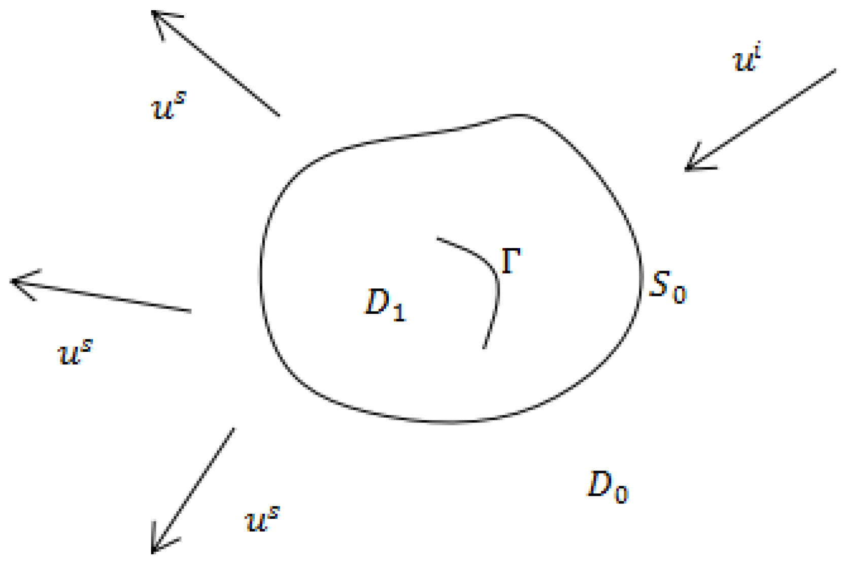This kind of inverse scattering problem with a crack has a wide range of applications in practical problems, such as non-destructive detection and medical imaging [22]. The schematic diagram of the inverse scattering problem of a crack is shown in Figure 1.

Figure 1. Schematic diagram of the inverse scattering problem.

Let $D_1$ be a bounded and simply connected domain of $R^2$ with a $C^2$ boundary $S_0$. We use $D_0$ to indicate the exterior domain of $D_1$, namely, $D_0=R^2\backslash {\overline{D}}_1$. The crack $\mathsf{\Gamma }$ is a open arc in $R^2$.

In the figure, $u^i$ denotes a time-harmonic incident plane wave and $u^s$ denotes the scattered wave field. In order to solve the inverse scattering problem of the crack, the mathematical model of the crack direct scattering problem is given below:

$$\begin{array}{c}\hfill \left\{\begin{array}{ccc}\hfill \Delta u\left(x\right)+{k_0}^2{n}_{0}u\left(x\right)& =& 0,\mathrm{in}{D}_0,\hfill \\ \hfill \Delta u\left(x\right)+{k_0}^2{n}_{1}u\left(x\right)& =& 0,\mathrm{in}{D}_1\backslash \mathsf{\Gamma },\hfill \\ \hfill u_{+}\left(x\right)-u_{-}\left(x\right)& =& 0,\mathrm{on}{S}_0,\hfill \\ \hfill \frac{\partial u_{+}\left(x\right)}{\partial v}-\frac{\partial u_{-}\left(x\right)}{\partial v}& =& 0,\mathrm{on}{S}_0,\hfill \\ \hfill u_{\pm }\left(x\right)& =& 0,\mathrm{on}\mathsf{\Gamma },\hfill \end{array}\right.\end{array}$$

(1)

where the total field $u\left(x\right)=u^i\left(x\right)+u^s\left(x\right)$, $u^s\left(x\right)$ is the scattering field, $u^i\left(x\right)=e^{i{k}_{0}x·d}$ is the incident field, and $k_0$ is the wave number. Here, $i=\sqrt{-1}$ is an imaginary unit, $d=\left(cos\right(\theta ),sin(\theta \left)\right)$ represents the incident direction, and $\theta$ is incident angle. Supposing the refractive index $n_1$ in $D_1$ is a constant and $n_1\ne 1$, the refractive index in $D_0$ is $n_0=1$, and v signifies the unit outward normal vector of the interface $S_0$. $u_{\pm }\left(x\right),\frac{\partial u_{\pm }\left(x\right)}{\partial v},$ have the following expressions:

$$u_{+}\left(x\right):=\underset{x\to x_0}{lim}u\left(x\right),\frac{\partial u_{+}\left(x\right)}{\partial v}:=\underset{x\to x_0}{lim}\frac{\partial u\left(x\right)}{\partial v},x\in D_0,x_0\in S_0,$$

$$u_{-}\left(x\right):=\underset{x\to x_0}{lim}u\left(x\right),\frac{\partial u_{-}\left(x\right)}{\partial v}:=\underset{x\to x_0}{lim}\frac{\partial u\left(x\right)}{\partial v},x\in D_1,x_0\in S_0.$$

In particular, $u^s\left(x\right)$ is required to satisfy the following Sommerfeld radiation condition at infinity:

$$\underset{r\to \infty }{lim}{r}^{\frac{1}{2}}(\frac{\partial u^s\left(x\right)}{\partial r}-ik{u}^s\left(x\right))=0,r:=\left|x\right|,$$

(2)

which holds uniformly in any observation direction $\widehat{x}=x/\left|x\right|$. Moreover, we know that the scattering field $u^s$ has the following asymptotic representation:

$$u^s\left(x\right)=\frac{e^{\mathrm{i}{k}_{0}r}}{r^{1/2}}\{u_{\infty }(\widehat{x};d)+\mathcal{O}\left(r^{-3/2}\right)\},r:=\left|x\right|\to +\infty .$$

(3)

$u^{\infty }(\widehat{x};d)$ is the far-field pattern with $\widehat{x}=x/\left|x\right|$. $u^{\infty }$ is actually a vector whose components are obtained under different observation directions. It can be seen that both $u^{\infty }(\widehat{x};d)$ and $u^s\left(x\right)$ are related to $\widehat{x}$ d. The crack scattering problem is to obtain the far-field data through the incident field and the crack $\mathsf{\Gamma }$. The inverse scattering problem of the crack is to reconstruct the geometric information of the crack by the incident field and far-field data.

Some scholars have carried out associated studies. Guo et al. extended the factorization method to the reconstruction problem of the crack shape in an inhomogeneous medium and theoretically demonstrated its feasibility [23]. To the best of our knowledge, the study of the inverse scattering problem with a crack is mainly at the theoretical stage, and there are few corresponding numerical algorithms.

Neural networks with a strong self-learning ability are suitable for dealing with nonlinear problems; therefore, they have good performance in the field of inverse problems. Gao et al. constructed a fully connected neural network that can recover obstacles or media using limited-aperture data, and that is more stable compared to traditional numerical methods [24]. Ji et al. used a generalized neural network to invert the resistivity and roughness of a rough medium, and the method could achieve a higher accuracy in a multilayer model [25]. Ossandón et al. designed a radial basis neural network with a lower computational cost than the finite element method to solve the inverse eigenvalue problem of the Laplacian operator [26]. Chuah built an inverse scattering model based on neural network, which can estimate multiple parameters of vegetation simultaneously within a 10% accuracy range [27]. Zhou et al. proposed a new neural network based on a linear model, which has realized a better reconstruction effect than the Born approximation algorithm and the sub-space optimization method [28]. Martin et al. proposed a neural network to solve the inverse problem of electrical impedance tomography; it provides high-quality lung imaging results and high robustness to noise [29]. Meng et al. constructed a shape parameters inversion model of the obstacle based on a neural network and accurately reconstructed the boundary shapes of obstacles [30]. Yin et al. presented a two-layer sequence-to-sequence neural network that can reconstruct the shapes of obstacles using phaseless data [31]. For more articles about neural networks solving inverse problems, please refer to [32,33,34,35,36]. Jin et al. put forward a new algorithm based on deep convolutional neural network to solve the ill-posed inverse problem, and the experiments proved that the method works well [37]. In recent years, the convolutional neural network, as one of the important representatives of deep learning, has received considerable attention. In this paper, we use CNN to solve the crack inversion problem in an inhomogeneous medium.

The rest of the paper is arranged as follows. Section 2 introduces the architecture of the neural network, as well as its inversion process, in detail. In Section 3, we demonstrate the effectiveness of the neural network through numerical experiments. In Section 4, we summarize the work of this paper and present a related discussion.

2. Construction of the Crack Inversion

Before describing the specific network architecture of the crack shape inversion, we first explain the expression of the crack.

In what follows, for the observation directions $d=\left(cos\right(\alpha ),sin(\alpha \left)\right)$, the observation angle $\alpha$ is uniformly distributed over $[\beta ,{\beta }^{{}^{\prime }}]$:

$$\alpha =({\alpha }_0,{\alpha }_1,\dots ,{\alpha }_n).$$

Here, ${\alpha }_l={\alpha }_0+\tau \lambda$, $\tau =1,\dots ,n$, $\lambda =[\beta ,{\beta }^{{}^{\prime }}]/n$, ${\alpha }_0=\beta$, and $n+1$ is the number of observation directions.

We use the observation angle $\alpha ={\alpha }_j$, and the corresponding far-field data are represented by $x_j,j=0,1,\dots ,n$. Hence, given $n+1$ observation directions, the far-field data can be expressed as

$$u_{\infty }=(x_1,x_2,\dots ,x_n)\in C^{1\times (n+1)}.$$

Here, $u_{\infty }$ is a complex vector, where each component $x_j=a_j+i{b}_j,j=0,1,\dots ,n$, and i is an imaginary unit.

Considering the scattering problem of acoustic waves from a crack in an inhomogeneous medium, we suppose that the boundary curve of the crack has the following parametric representation:

$$z=z\left(s\right),s=[-1,1].$$

Here, $z:=[-1,1]$→${\mathbb{R}}^2$ is a continuously differentiable injective function. Let $h,h^{\prime }$ denote the two tip points of the crack, assuming that the direction of $\mathsf{\Gamma }$ is from h to $h^{\prime }$. Consequently, in terms of the direction of $\mathsf{\Gamma }$, we denote by ${\mathsf{\Gamma }}_{-1},{\mathsf{\Gamma }}_1$ the convergence to the crack from the left and right, respectively. $z\left(s\right)$ is represented by the following truncated Fourier series:

$$z\left(s\right)=\frac{y_0}{2}+\underset{q=1}{\overset{Q}{\Sigma }}{y}_{2q-1}cos\left(qs\right)+\underset{q=1}{\overset{Q}{\Sigma }}{y}_{2q}sin\left(qs\right).$$

(4)

Here, $Q\in \mathbb{N}$, namely, the vector $y=(y_0,y_1,\dots ,y_{2Q})$$\in R^{2Q+1}$ is the shape parameter of the crack. In fact, the shape parameter is in the form of the sequence. The forward problem is solved using the finite element method to obtain the far-field pattern data. The aim of this paper is to construct a sequence-to-sequence neural network, and to play on the far-field data $u_{\infty }$ to invert the shape parameter y, so as to determine the shape of the crack. The CNN structure of the inverse scattering problem with a crack is given below. In order to conveniently introduce the network structure, the following three definitions are first presented.

Definition 1. 

Let $A=\left(\begin{array}{cccc}{a}_{11}& a_{12}& \cdots & a_{1m}\\ ⋮& ⋮& & ⋮& \\ a_{n1}& a_{n2}& \cdots & a_{nm}\end{array}\right)\in R^{n\times m},B=\left(\begin{array}{cccc}{b}_{11}& b_{12}& \cdots & b_{1m}\\ ⋮& ⋮& & ⋮& \\ b_{p1}& b_{p2}& \cdots & b_{pm}\end{array}\right)\in R^{p\times m},$ then define the operation as follows:

$$\begin{array}{c}=\left(\begin{array}{cccc}{a}_{11}& a_{12}& \cdots & a_{1m}\\ ⋮& ⋮& & ⋮& \\ a_{n1}& a_{n2}& \cdots & a_{nm}\\ b_{11}& b_{12}& \cdots & b_{1m}\\ ⋮& ⋮& & ⋮& \\ b_{p1}& b_{p2}& \cdots & b_{pm}\end{array}\right)\in R^{(n+p)\times m}.\end{array}$$

Definition 2. 

Assuming that the data obtained in the observation direction d = $(cos({\alpha }_j)$, $sin\left({\alpha }_j\right))$ are $x_j=a_j+i{b}_j,j=0,1,\dots ,n$, the following operation is defined:

$$[a_j,b_j]=(a_j,b_j),[x_j,x_{j+1}]=(x_j,x_{j+1}).$$

Definition 3. 

Assuming that $A=(a_1,a_2,\dots ,a_m)\in R^m$, $F\left(A\right)$ is

$$F\left(A\right)=(F\left(a_1\right),F\left(a_2\right),\dots ,F\left(a_m\right)).$$

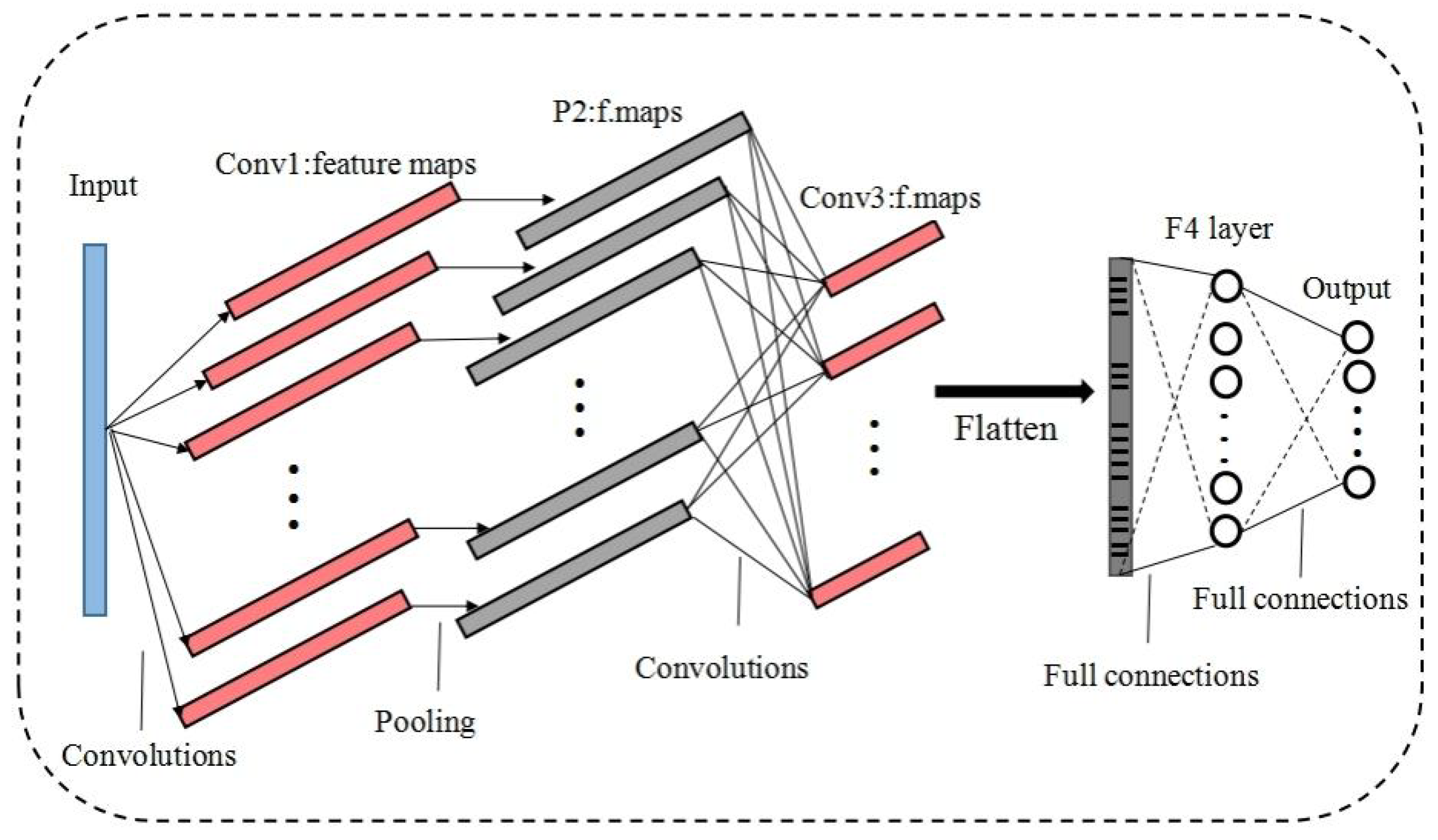
Next, we construct a CNN for the inversion of the shape parameter y; its structure is shown in Figure 2. The network consists of two convolutional layers, one pooling layer and two fully connected layers.

Figure 2. CNN structure of cracks inversion.

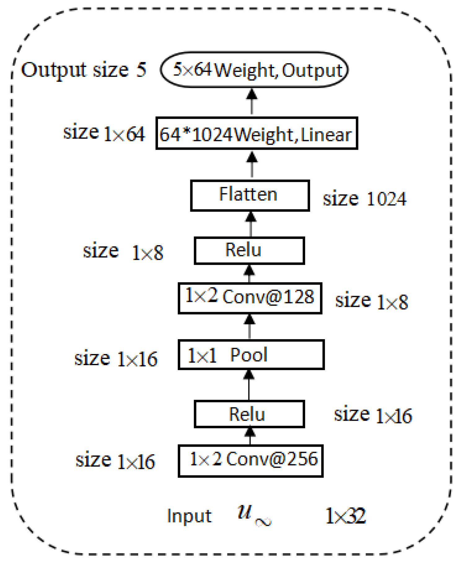
It can be known that the far-field data of $n+1$ observation directions can be written as $u_{\infty }=(a_0,b_0,\dots ,a_n,b_n)=(c_1,c_2,\dots ,c_{2n+2})\in R^{1\times 2(n+1)}$. Next, we take $n=15,Q=2$ as an example to illustrate the inversion process of the shape parameters y, and the specific structure is shown in Figure 3.

Figure 3. Flow chart of cracks inversion.

Here, the left side of @ represents the size of the convolution kernel or pooling kernel and the right side of @ represents the number of convolution kernels or pooling kernels in the layer.

The far-field data $u_{\infty }=(c_1,c_2,\dots ,c_{32})$ are regarded as the input of the network, the convolution kernel $W_1=(w^1,w^2)\in R^{1\times 2}$ is randomly initialized without a loss of generality, and all biases are set to 0. The convolution operation ∗ for the input sequence $u_{\infty }$ and the convolution kernel $W_1$ is as follows:

$$z_m=W_1\ast u_{\infty }=(w^1,w^2){(c_{2m-1},c_{2m})}^T=w^1{c}_{2m-1}+w^2{c}_{2m},m=1,2,\dots ,16.$$

(5)

It can be seen from the above formula that $W_1$ slides to the right on the input sequence $u_{\infty }$ with a sliding step size of 2. Each slide performs a convolution calculation as in formula (5), and finally, the vector $z=(z_1,z_2,\dots ,z_{16})$∈$R^{1\times 16}$ is outputted. The convolution process is as depicted in Figure 4.

Figure 4. Diagram of convolution.

If the layer has k convolution kernels, $k\in R^{+}$, namely, $u_{\infty }$ has k output channels after the first convolution layer and the k output vectors are written as $(z^1,z^2,\dots ,z^k)$, the output of the first layer is passed to the nonlinear activation function F, which selects $ReLU$.

$$F=ReLU=max(x,0),x\in R,$$

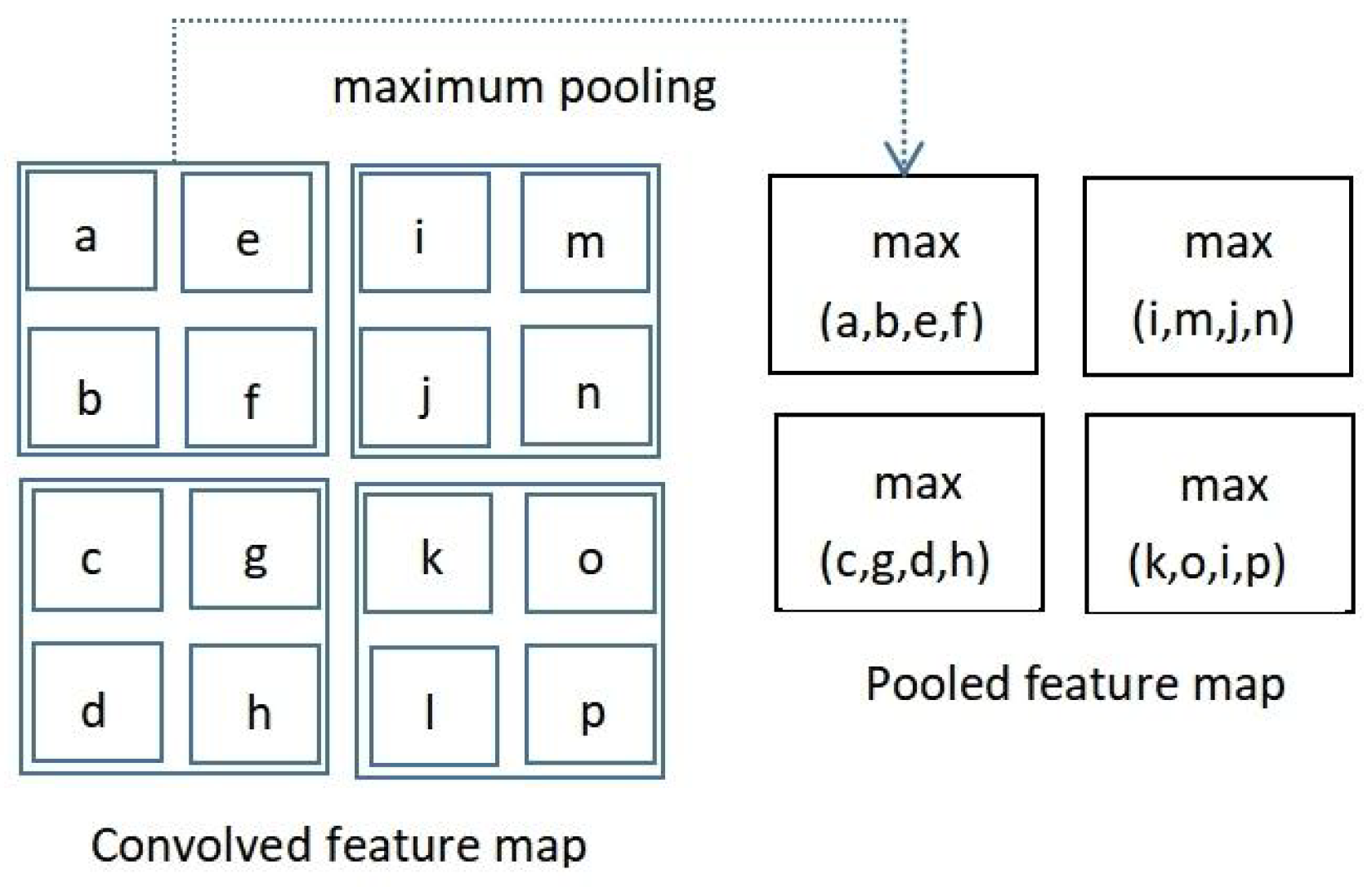
where $x=(z^1,z^2,\dots ,z^k)$ is the input of the activation function. It can be seen from Definition 3 that the dimension of the output vector remains changeless after activation. The result of the activation is passed to the pooling layer, where the $1\times 1$ pooling kernel divides the input data into 16 feature areas. The max value of each area is selected as an output vector $p\in R^{1\times 16}$. As shown in Figure 5, the pooling layer is divided into four feature areas. The same pooling method is used for k inputs to gain k outputs of the same dimension.

Figure 5. Diagram of max-pooling.

The output of the pooling layer is indicated as $p_1,p_2,\dots ,p_k$$\in R^{1\times 16}$, and it is handed to the second convolutional layer. For sequences with multiple input channels, a convolution kernel $W_2=(t^1,t^2,\dots ,t^k)$ with k channels is randomly initialized, and each channel in the convolution kernel is $t^1,t^2,\dots ,t^k\in R^{1\times 2}$. The operation of this convolutional layer is as follows:

$$Z_m=t^1\ast p_1+t^2\ast p_2+\cdots +t^k\ast p_k,m=1,2,\dots ,8.$$

(6)

Here, the convolution ∗ operation is as in (5); each sliding performs a convolution calculation as in formula (6), finally obtaining the output $Z=(Z_1,Z_2,\dots ,Z_8)$$\in R^{1\times 8}$. If there are q convolution kernels in the current layer, and each convolution kernel operates with the input sequence as in (6), the layer obtains q outputs, which are recorded as $Z^1,Z^2,\dots ,Z^q$$\in R^{1\times 8}$. Similarly, the input data remain unchanged though the $ReLU$ activation function. After the process of convolution–pooling–convolution, q feature vectors are extracted. The result of feature extraction can be spliced into $X=(Z^1,Z^2,\dots ,Z^q)$$\in R^{1\times 8q}$ via Definition Section 2. The fully connected layer randomly initializes the convolution kernel $W_3\in R^{64\times 8q}$, and the operation is as follows:

$$f=X{W_3}^T.$$

(7)

By means of the second fully connected layer, the input data X obtain the output $f\in R^{1\times 64}$. The output layer randomly initializes the convolution kernel $W_4=R^{5\times 64}$ for the input sequence f, and performs the same operation as (7) to acquire the result. The result of the output layer is recorded as $y^{\prime }\in R^5$, where the dimension of $y^{\prime }$ stands for the number of shape parameters of the crack. There is an error between the network output $y^{\prime }$ and the y corresponding to the far-field data $u_{\infty }$, and the following mean square error is regarded as the loss function $L:$

$$L(Y,Y^{\prime })=\frac{1}{n}\underset{j=1}{\overset{n}{\Sigma }}{\left|\right|Y_j-{Y_j}^{\prime }\left|\right|}^2.$$

(8)

Here, n is the total number of samples to be calculated, $Y_j$ represents the real shape parameter of the j-th sample, and ${Y_j}^{\prime }$ is the shape parameter of the corresponding sample inversed by the CNN, $j=1,2,\dots ,n$.

Let $W=(W_1,W_2)$ be the weight of the CNN, with $W_1$ and $W_2$ on behalf of the convolution kernel of the first and second convolutional layers, respectively. W is initialized to $W_0$; then, it is gradually updated to $W_l$ using the Adam optimization algorithm, where $l=1,2,\dots$. The main steps of the algorithm are as follows:

$$g_l={\nabla }_{W}L(Y,Y^{\prime }\left(W^l\right)),$$

$$m_l={\alpha }_1{m}_{l-1}+(1-{\alpha }_1)g_l,$$

$$v_l={\alpha }_2\ast v_{l-1}+(1-{\alpha }_2)g_l\otimes g_l,$$

$${\widehat{m}}_l=m_l/(1-{{\alpha }_1}^l),$$

$${\widehat{v}}_l=v_l/(1-{{\alpha }_1}^l),$$

$$\Delta W_l=-\zeta \frac{{\widehat{m}}_l}{\sqrt{{\widehat{v}}_l+\epsilon }},$$

$$W_l=W_{l-1}+\Delta W_l,$$

where $g_l$ is the gradient matrix obtained by deriving the objective function L with respect to the parameter W. $m_l$ and $v_l$ are the first- and second-order moment estimates of the gradient $g_l$, respectively, and their initial values are both zero vectors. ${\alpha }_1,{\alpha }_2\in [0,1)$ are the exponential attenuation rates of the first- and second-order moment estimates, respectively. ${\widehat{m}}_l$ and ${\widehat{v}}_l$ are the modified first- and second-order biased moment estimates, respectively. $\zeta$ is the learning rate selected to regulate the update step of the parameter, and $\epsilon$ is a very small constant. The kernel parameters are updated through backpropagation, and y’ is trained repeatedly to approximate the real shape parameters of the crack.

3. Results of the Numerical Experiment

In this section, we will demonstrate the effectiveness of the proposed neural network for the inverse scattering problem of the crack through several numerical experiments. We obtain the far-field data via the finite element method through the incident field and the crack $\mathsf{\Gamma }$. From Equation (4), the crack can be expanded into a Fourier series, and the parameter expression of the crack to be inversed in this section is shown below:

$$z_1\left(s\right)=a_0+a_{1}cos\left(s\right)+a_{2}sin\left(s\right)+a_{3}cos\left(2s\right)+a_{4}sin\left(2s\right),s\in [0,\pi /2].$$

The above equation shows that the shape parameter of the crack is $Y=(a_0,a_1,a_2,a_3,a_4)\in R^5$. In the numerical experiment, we consider an M set of cracks with different shapes, and the shape parameters are denoted as $Y^{\mathsf{\Gamma }}=(a_0^{\mathsf{\Gamma }}$,$a_1^{\mathsf{\Gamma }}$,$a_2^{\mathsf{\Gamma }}$,$a_3^{\mathsf{\Gamma }}$,$a_4^{\mathsf{\Gamma }})$, $\mathsf{\Gamma }=1,2,\dots ,M$. If there are N observation directions, the corresponding far-field data can be written as $u_{\infty }^{\mathsf{\Gamma }}=(c_1^{\mathsf{\Gamma }}$,$c_2^{\mathsf{\Gamma }},\cdots$,$c_{2N}^{\mathsf{\Gamma }}$). Then, M samples are taken as the dataset for our experiments, and the training dataset of the model can be defined as

$$\mathrm{T}=\left\{(u_{\infty }^{\mathsf{\Gamma }},Y^{\mathsf{\Gamma }})\right|u_{\infty }^{\mathsf{\Gamma }}\in R^{1\times 2N},Y^{\mathsf{\Gamma }}\in R^5,\mathsf{\Gamma }=1,2,\dots ,M\}.$$

Here, $u_{\infty }^{\mathsf{\Gamma }},Y^{\mathsf{\Gamma }}$ represent the far-field data and the shape parameters related to the crack, respectively.

For ease of calculation, we have the following setups in all of the numerical examples below. Due to the range of solutions set using the PML technique, we set the range of crack shape parameters to $a_0\in (-1,1),a_1,a_2,a_3,a_4\in (-2,2)$. Only a single incident wave is used in the experiment, and the wave number is $k=2$. The number of neurons in the CNN is generally set to $2^l,l\in Z^{+}$; our experiment takes $l=7$ and 8. For the choice of other network parameters, we refer to [31]. The parameter settings of the network are shown in Table 1.

Table 1. Hyperparameter settings.

Parameter	Parameter Value
Number of neurons CNN in the first convolution	256
Number of neurons CNN in the second convolution	128
Batch	256
Epoch	300
Learning rate	0.001

Example 1. 

Reconstruction of cracks under different data volumes.

In this experiment, we set the incident direction of the plane acoustic wave $u^i$ as $d=(1,0)$ and consider the inversion of crack

$$z\left(s\right)=-0.42-1.06cos\left(s\right)+1.28sin\left(s\right)-0.44cos\left(2s\right)+0.75sin\left(2s\right),s\in [0,\pi /2].$$

The number of observation directions is 16, and these are evenly distributed on the circle; the data volumes of the training set in the following figures are 2000, 5000, 10,000, and 20,000, respectively.

As can be seen from Figure 6, with an increase in the data volumes, the effects of reconstruction are obviously gradually improved while also bringing a higher calculation cost. We found that when the data volumes are 10,000, the inversion effect is acceptable and there are no special instructions; the subsequent experiments use 10,000 data volumes. Taking the mean square error between the real and the predicted curve in the crack reconstruction results, the following Table 2 is obtained.

Figure 6. Reconstruction of a crack under different data volumes: (a) 2000 data volumes; (b) 5000 data volumes; (c) 10,000 data volumes; (d) 20,000 data volumes.

Table 2. Errors corresponding to different training data volumes.

Training Data Volumes	2000	5000	10,000	20,000
MSE	0.01	8.31 × ${10}^{-5}$	6.93 × ${10}^{-5}$	2.21 × ${10}^{-5}$

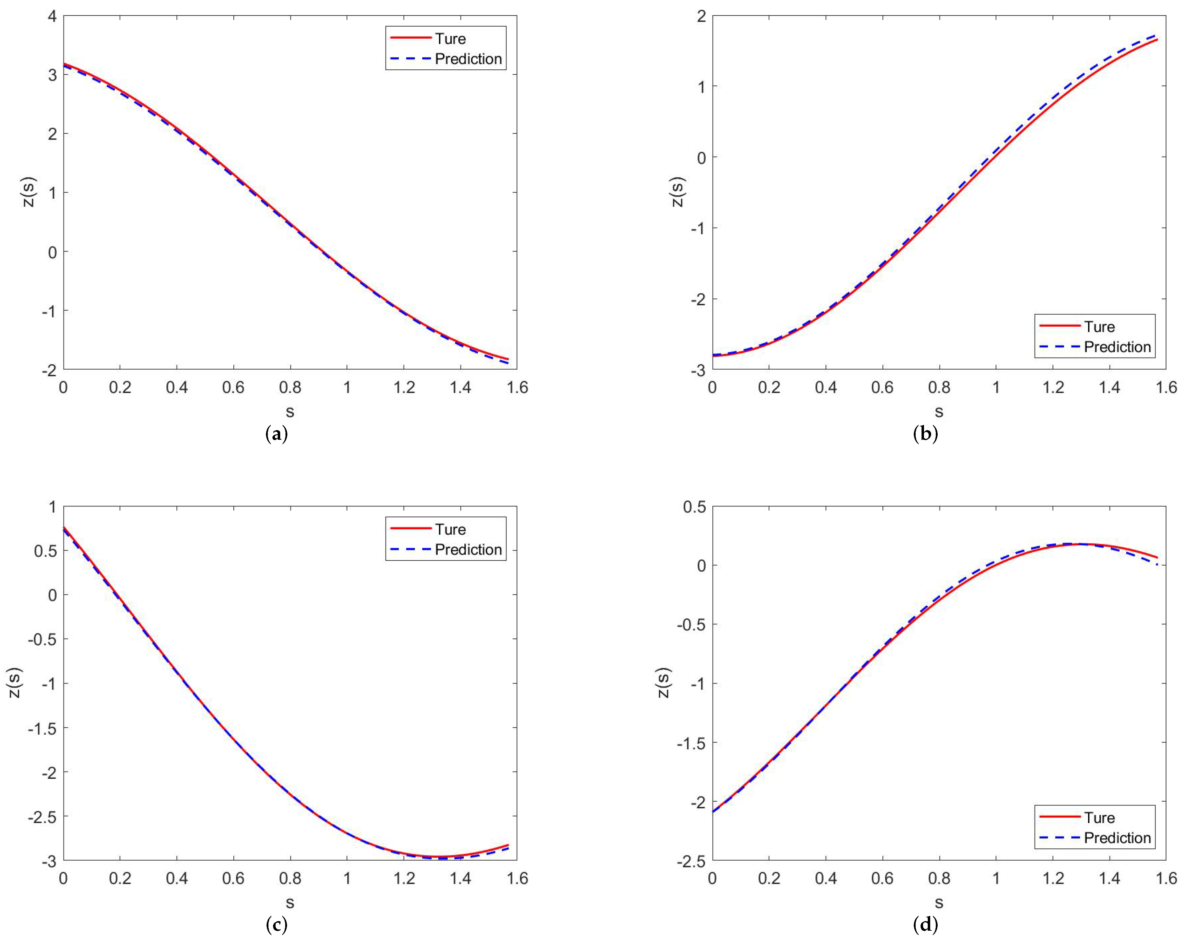
Example 2. 

Reconstruction of cracks with different shapes under full aperture.

In this experiment, we set the incident direction $d=(1,0)$ of the plane acoustic wave $u^i$, and we consider the inversion of the following four shapes of cracks. The number of observation directions is 16, and these are evenly distributed on the circle; the expressions of cracks are as follows:

$$z_1\left(s\right)=0.37+1.32cos\left(s\right)-1.65sin\left(s\right)+1.56cos\left(2s\right)+0.04sin\left(2s\right),s\in [0,\pi /2],$$

$$z_2\left(s\right)=0.46-1.87cos\left(s\right)-0.20sin\left(s\right)-1.40cos\left(2s\right)+0.17sin\left(2s\right),s\in [0,\pi /2],$$

$$z_3\left(s\right)=-0.57+0.96cos\left(s\right)-1.89sin\left(s\right)+0.37cos\left(2s\right)+0.99sin\left(2s\right),s\in [0,\pi /2],$$

$$z_4\left(s\right)=-0.76-0.77cos\left(s\right)+0.25sin\left(s\right)-0.56cos\left(2s\right)+0.80sin\left(2s\right),s\in [0,\pi /2].$$

It can be seen from Figure 7—for 10,000 data volumes, 16 observation points, and other identical experimental settings—that just by changing the shapes of the cracks, we found our method works equally well for different shapes of cracks.

Figure 7. Reconstruction of a crack under different data volumes. (a) Reconstruction effect of $z_1\left(s\right)$. (b) Reconstruction effect of $z_2\left(s\right)$. (c) Reconstruction effect of $z_3\left(s\right)$. (d) Reconstruction effect of $z_4\left(s\right)$.

Example 3. 

Reconstruction of the crack under different observation directions.

In this experiment, we set the incident direction $d=(1,0)$ of the plane acoustic wave $u^i$, and consider the inversion of crack

$$z\left(s\right)=0.02+0.62cos\left(s\right)-0.52sin\left(s\right)+0.34cos\left(2s\right)-0.06sin\left(2s\right),s\in [0,\pi /2].$$

Take $[\beta ,{\beta }^{{}^{\prime }}]=[0,2\pi ]$, and take $n=31,15,7$ under this aperture, respectively, according to the inversion effect of cracks with different shapes to analyze. Figure 8 shows the relationship between the loss function and the number of iterations at different observation points.

Figure 8. Reconstruction of the crack under different observation points: (a) 32 observation points; (b) 16 observation points; (c) 8 observation points; (d) loss function at different observation points.

The experiments show that with an increase in the number of observation points, more far-field information is obtained, and the reconstruction effect of the crack shape gradually becomes better.

Example 4. 

Reconstruction of the crack under different noise data.

In this experiment, we prove the robustness of our network. For this reason, the number of observation directions is taken to be 16 and is uniformly distributed on the circle. We consider a network with 30,000 training shapes to reconstruct the crack shape under different noises; the shape of the crack in Figure 9 is

$$z\left(s\right)=0.97-0.28cos\left(s\right)-0.28sin\left(s\right)+0.56cos\left(2s\right)+0.07sin\left(2s\right),s\in [0,\pi /2].$$

Figure 9. Reconstruction of the crack under different observation points. (a) Reconstruction effect under 0% noise. (b) Reconstruction effect under 5% noise. (c) Reconstruction effect under 10% noise. (d) Reconstruction effect under 20% noise.

We take $[\beta ,{\beta }^{{}^{\prime }}]=[0,2\pi ]$, and on this condition, we take n = 15. The shape and location of the crack were reconstructed, and 5%, 10%, and 20% Gaussian noise was added to the testing data, respectively. It can be seen from the above figure that noise has an impact on crack inversion, and that the experimental effect shows that the network has a certain degree of stability as the noise increases.

Example 5. 

Reconstruction of the crack under limited-aperture data.

In this experiment, the direction of the plane incident wave is set as $d=(-1,0)$. The number of observation directions is taken to be 16 and is uniformly distributed on the circle. We consider the inversion of crack in Figure 10 as

$$z=0.92+1.94cos\left(s\right)-1.71sin\left(s\right)-0.52cos\left(2s\right)+0.06sin\left(2s\right)).$$

Figure 10. Reconstruction of the crack under different apertures. (a) Reconstruction effect under aperture [0, 2$\pi$]. (b) Reconstruction effect under aperture [$-\pi$/2, $\pi$/2]. (c) Reconstruction effect under aperture [$-\pi$/4, $\pi$/4]. (d) Reconstruction effect under aperture [$-\pi$/8, $\pi$/8].

Taking different apertures, $[{\beta }_1,{{\beta }_1}^{{}^{\prime }}]=[0,2\pi ]$, $[{\beta }_2,{{\beta }_2}^{{}^{\prime }}]=[-\pi /2,\pi /2]$, $[{\beta }_3,{{\beta }_3}^{{}^{\prime }}]=[-\pi /4,\pi /4]$, $[{\beta }_4,{{\beta }_4}^{{}^{\prime }}]=[-\pi /8,\pi /8]$. Taking n = 15 under the four apertures to reconstruct the shape and location of the crack, the experiments are made known as the observation aperture gradually becomes smaller, namely, a lack of far-field information that will lead to gradual worsening of the inversion effect in the limited aperture.

Example 6. 

Reconstruction of two cracks.

In this experiment, the reconstruction of a single crack is extended to the case of two cracks, and the direction of the plane incident wave is set as $d=(1,0)$. The number of observation directions is taken to be 32, which are uniformly distributed on the circle, and we consider the inversion of the crack as

$$z1=-0.52-0.66cos\left(s\right)-1.44sin\left(s\right)+1.46cos\left(2s\right)+0.85sin\left(2s\right)),$$

$$z2=-0.7-1.04cos\left(s\right)-0.92sin\left(s\right)-0.85cos\left(2s\right)-1.41sin\left(2s\right)),$$

$$z3=-0.14-0.74cos\left(s\right)-1.66sin\left(s\right)-0.84cos\left(2s\right)+1.31sin\left(2s\right)),$$

$$z4=-0.76-0.09cos\left(s\right)-0.91sin\left(s\right)+1.04cos\left(2s\right)-0.78sin\left(2s\right)).$$

In Figure 11, we can see that when the number of cracks is two, parameters of the network inversion increase, resulting in an unsatisfactory inversion effect.

Figure 11. Reconstruction of two cracks. (a) Reconstruction effect of cracks $z1$ and $z2$. (b) Reconstruction effect of cracks $z3$ and $z4$.

4. Conclusions

In this paper, we considered the inverse acoustic scattering problem of a crack in a highly challenging environment with limited-aperture far-field data and inhomogeneous medium. In addition, the collected far-field data only correspond to an incident wave. Taking the inverse acoustic scattering problem of the crack as a working model, we set up a neural network scheme to efficiently solve the reconstruction problem in these challenging situations. Our numerical experiments show some very attractive features of the proposed method, such as its simplicity and direct nature. Moreover, the convergence of the proposed network is verified in numerical experiments. Our study paves the way for any interesting extensions, including the more realistic inverse electromagnetic scattering problem dominated by Maxwell’s system. We will consider these extensions in future studies.