Analysis of a Squeezing Flow of a Casson Nanofluid between Two Parallel Disks in the Presence of a Variable Magnetic Field

Abstract

The present article deals with the MHD flow of a Casson nanofluid between two disks. The lower disk was fixed as well as permeable. The upper disk was not permeable, but it could move perpendicularly up and down toward the lower disk. Titanium dioxide was selected as nanoparticles and water as a base fluid. The governing higher-order nonlinear partial differential equations were transformed into a set of nonlinear ordinary differential equations by using similarity transformation. The differential transform method (DTM) was applied to solve the nonlinear ODEs. The nature of the velocity profiles for the different values of the suction injection parameter, the squeeze number, the Casson fluid parameter, and the volume fraction parameter of the nanofluid are pictorially discussed in this paper. The coefficient of skin friction was tabulated for the novelty of the research. The comparison of the results was determined by the DTM and the numerical methods. The profile values were also compared with the literature work and found to agree. This comparative study proves the accuracy and efficiency of the method. It is concluded from this research that the flow properties behave oppositely for all parameters during suction and injection.

1. Introduction

Continuous research is being carried out on the squeezing flow between parallel disks. Considering its biological and industrial applications, numerous academics are interested in studying this topic. Numerous initiatives have been made to completely understand these types of flow. Piston movement is essential for the operation of machinery and engines. Nasogastric tubes and syringes both use a moving disk to squeeze the flow of the fluid. Stefan [1] identified the first model for squeezing flow. After his discovery, many scientists studied and investigated new findings of squeezing flow. Leider and Bird [2] investigated the same flow for the parallel disks. Many mathematical flow problems involve non-Newtonian fluids. Casson fluid is one of them. Casson fluid exhibits yield stress. It is a shear-thinning liquid. It is assumed to have infinite viscosity at zero rate shear. If yield stress is more than the shear stress, it behaves like a solid, and if it is less than the shear stress, it starts to move. Some examples of such fluids are jelly, tomato ketchup, soup, honey, etc. In the past decade, many scientists discussed the squeezing flow model for different fluids such as Jeffery fluid, Casson fluid, second-order fluid, micropolar fluid, etc. Qayyum et al. [3] investigated the flow of Jeffery fluid, squeezed between parallel disks. They applied the series solution method to find the solution. Mohyud-Din and Khan [4] presented the radiation effects of Casson fluid, flowing between parallel disks. They considered one porous disk and adopted HAM to obtain the solution of profile expression. Song et al. [5] investigated nanofluid flow over a vertical thin needle. They presented thermophoresis and the Brownian motion effect in their study. Naveed et al. [6] considered the flow of Casson fluid squeezing between two parallel disks. They presented a comparison of two method results for validation. Hussain and Xu [7] performed the analysis of a micropolar fluid. They considered one moving and one fixed disk. They discussed the effect of the various physical parameters on profiles. Khan et al. [8] addressed Carreau–Yasuda fluid on porous media. They also considered mixed convection. They solved obtained equations by the shooting method.

A particle having a diameter less than 100 nm is said to be a nanoparticle, and a fluid formed by such nanoparticles is known as a nanofluid. Choi [9] first showed that incorporating these nanoparticles into the base fluid improved thermal conductivity. Eastman et al. [10] studied the characteristics of the heat transfer of nanocrystalline particles in water or oil as a base fluid. Xu et al. [11] considered the effect of the Prandtl number in nanofluid and solved it numerically. Hashmi et al. [12] investigated the MHD flow of nanofluid compressed between parallel disks. They used HAM to determine the solution. Dinarvand et al. [13] studied the MHD flow of a hybrid nanofluid with thermal radiation. They discussed the different directions of the needle. Further research has been conducted by Hayat et al. [14], Berrehal et al. [15], and Agarwal [16,17,18,19]. Many authors applied HPM, HAM, etc., in their research. We opted here to apply DTM because DTM does not depend on small parameters such as $p$ in HPM. Therefore, DTM can be applied regardless of whether the governing equations and BVPs and IVPs contain small or large amounts. Like HAM, DTM does not need to find auxiliary functions and parameters or adequate initial guesses. This method was first developed by Zhou [20] in the electric circuit. DTM is based on Taylor’s series and produces a polynomial as a result. DTM differs from the traditional higher-order Taylor series method, which requires the symbolic computation of the required derivatives of the data function. Additionally, the skills of this method have led many authors to use this method to solve nonlinear equations. Usman et al. [21], Hatami et al. [22], and Sheikholeslami and Ganji [23] applied DTM in their research.

The present research is devoted to finding the MHD flow characteristics of Casson nanofluid, which is moving up and down vertically between two parallel disks. The lower disk is considered fixed but permeable while the upper disk is moving perpendicularly and nonpermeable. The obtained equations of mathematical problems are solved by using DTM. The effect of different parameters is discussed and presented graphically. The skin friction coefficient is also tabulated in the study.

2. Mathematical Analysis

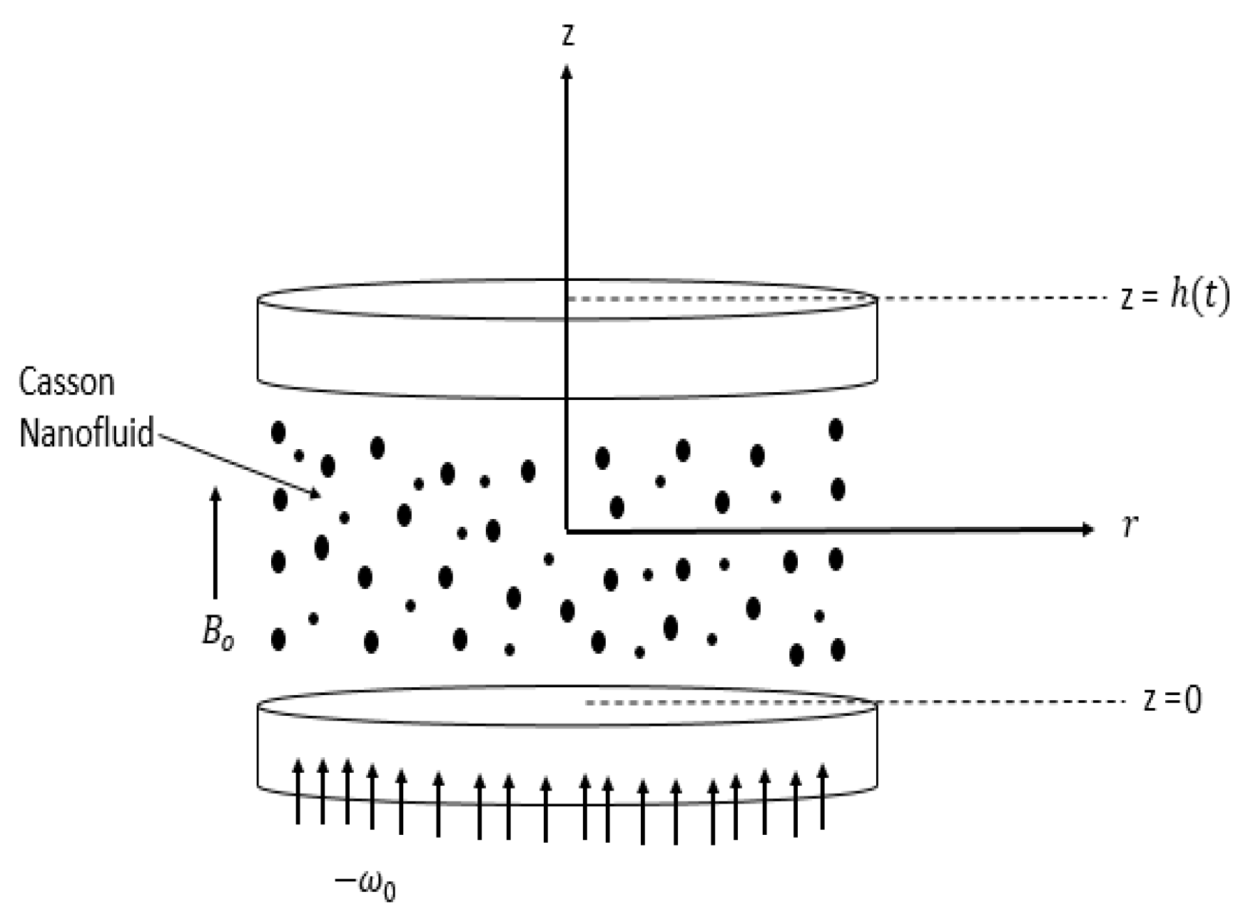
An axisymmetric 2D flow of a noncompressible Casson nanofluid between two parallel disks $h\left(t\right)\left[=H\sqrt{\left(1-at\right)}\right]$ distance apart is considered. The magnetic field with intensity $B\left(t\right)\left[\propto B_o\sqrt{1-at}\right]$ is vertically applied on disks as shown in Figure 1. The upper disk lies on $z=h\left(t\right)$ plane and is considered a moving disk. This disk is moving with velocity $\frac{a}{2}h\left(t\right)$ in the perpendicular direction.

The Casson fluid equation [4] is defined as

$${\tau }_{ij}=\left\{\begin{array}{c}2\left[{\mu }_B+\left(\frac{P_y}{2{\pi }_c}\right)e_{ij}\right],\pi >{\pi }_c\\ 2\left[{\mu }_B+\left(\frac{P_y}{2{\pi }_c}\right)e_{ij}\right],{\pi }_c>\pi \end{array}\right.$$

where $P_y$ is the stress of fluid, ${\mu }_B$ is the plastic dynamic viscosity of fluid, and ${\pi }_c$ is the critical value of the said self product $\pi$. A cylindrical coordinate system $(r,\theta ,z)$ is taken. Due to the symmetrical rotation, the velocity component along the $\theta$ direction is ignored. The basic equations for the 2D unsteady flow of the Casson nanofluid [6] are given by:

$$\frac{\partial \dot{u}}{\partial r}+\frac{\dot{u}}{r}+\frac{\partial \dot{w}}{\partial z}=0$$

(1)

$${\rho }_{nf}\left(\frac{\partial \dot{u}}{\partial t}+\dot{u}\frac{\partial \dot{u}}{\partial r}+\dot{w}\frac{\partial \dot{u}}{\partial z}\right)=-\frac{\partial p}{\partial r}+{\mu }_{nf}\left(1+\frac{1}{{\beta }_e}\right)\left(\frac{{\partial }^2\dot{u}}{\partial r^2}+\frac{1}{r}\frac{\partial \dot{u}}{\partial r}-\frac{\dot{u}}{r^2}+\frac{{\partial }^2\dot{u}}{\partial z^2}\right)-\frac{{\sigma }_{nf}}{{\rho }_{nf}}{B}^2\left(t\right)\dot{u}$$

(2)

$${\rho }_{nf}\left(\frac{\partial \dot{w}}{\partial t}+\dot{u}\frac{\partial \dot{w}}{\partial r}+\dot{w}\frac{\partial \dot{w}}{\partial z}\right)=-\frac{\partial p}{\partial z}+{\mu }_{nf}\left(1+\frac{1}{{\beta }_e}\right)\left(\frac{{\partial }^2\dot{w}}{\partial r^2}+\frac{1}{r}\frac{\partial \dot{w}}{\partial r}+\frac{{\partial }^2\dot{w}}{\partial z^2}\right)$$

(3)

The boundary conditions [6] are:

$$\dot{u}=0,\dot{w}=\frac{d}{dt}h\mathrm{at}z=0;\dot{u}=0,\dot{w}=-{\dot{\omega }}_0\mathrm{at}z=h\left(t\right)$$

(4)

Throughout the study, $\dot{u}$ and $\dot{w}$ represent components of velocity in the direction of $r$ and $z$, respectively. ${\rho }_{nf}\left[=\left(1-\varphi \right){\rho }_f+\varphi {\rho }_s\right],{\mu }_{nf}\left[=\frac{{\mu }_f}{{(1-\varphi )}^{2.5}}\right]$ and ${\sigma }_{nf}\left[={\sigma }_f\left\{1+\frac{3\left(\frac{{\sigma }_s}{{\sigma }_f}-1\right)\varphi }{\left(\frac{{\sigma }_s}{{\sigma }_f}+2\right)\varphi -\left(\frac{{\sigma }_s}{{\sigma }_f}-1\right)\varphi }\right\}\right]$ represent the effective density, viscosity, and electrical conductivity of the nanofluid. $p$ denotes the pressure term and ${\beta }_e$ denotes the Casson fluid parameter.

The similarity transformations [6] are:

$$\dot{u}=\frac{ar}{2\left(1-at\right)}{f}^{\prime }(\eta ),\dot{w}=-\frac{aH}{2{\left(1-at\right)}^{\frac{1}{2}}}f\left(\eta \right),B\left(t\right)=\frac{B_0}{{\left(1-at\right)}^{\frac{1}{2}}},\eta =\frac{Z}{h{\left(1-at\right)}^{\frac{1}{2}}}$$

(5)

Substitute Equation (5) in Equations (2) and (3). We eliminate $p$ from both equations, and finally, we obtain

$$\left(1+\frac{1}{{\beta }_e}\right)f^{iv}-S_x\left(1-\varphi +\varphi \frac{{\rho }_s}{{\rho }_f}\right){\left(1-\varphi \right)}^{2.5}\left(\eta f^{‴}+3f^{″}-2f{f}^{‴}\right)-{H_a}^2\left(1+\frac{3\left(\frac{{\sigma }_s}{{\sigma }_f}-1\right)\varphi }{\left(\frac{{\sigma }_s}{{\sigma }_f}+2\right)-\left(\frac{{\sigma }_s}{{\sigma }_f}-1\right)\varphi }\right){\left(1-\varphi \right)}^{2.5}{f}^{″}=0$$

(6)

With supported conditions:

$$f\left(0\right)=\alpha ,f^{\prime }\left(0\right)=0,f\left(1\right)=0.5,f^{\prime }\left(1\right)=0,$$

(7)

where $S_x\left[=\frac{{\rho }_{f}a{H}^2}{2{\mu }_f}\right]$ represents the squeeze number, $\alpha$ denotes the suction and injection parameter, and ${H_a}^2\left[=\frac{{\sigma }_f{B_0}^2{H}^2}{{\mu }_f}\right]$ denotes the Hartmann number.

The coefficient of the skin friction [4] is given by:

$$C_{sf}=\frac{{\left[{\tau }_{rz}\right]}_{z=h\left(t\right)}}{{\rho }_{nf}{\left(-\frac{aH}{2\sqrt{(1-at)}}\right)}^2}$$

where ${\tau }_{rz}={\mu }_{nf}{\left(\frac{\partial \dot{u}}{\partial z}+\frac{\partial \dot{w}}{\partial r}\right)}_{z=h\left(t\right)}$,

$$\therefore C_{sf}=\left(1+\frac{1}{{\beta }_c}\right)\frac{f^{″}\left(1\right)r^2}{H^2{R}_{er}},\mathrm{where}{R}_{er}=\frac{raH\sqrt{1-at}{\rho }_{nf}}{2{\mu }_{nf}}$$

(8)

3. Procedure of the Differential Transform Method

$k$ times differentiation of $f\left(x\right)$ in this method [20] is given by

$$\widehat{F}\left(k\right)=\frac{1}{k!}{\left(\frac{d^{k}f\left(x\right)}{d{x}^k}\right)}_{x=x_0}$$

(9)

The inverse transformation of $\widehat{F}(k)$ is defined by

$$f\left(x\right)={\displaystyle \sum }_{k=0}^{\infty }\widehat{F}\left(k\right){(x-x_0)}^k$$

(10)

$f\left(x\right)$ can be shown in the form of finite series and hence, Equation (10) can be stated as

$$f\left(x\right)={\displaystyle \sum }_{k=0}^n\widehat{F}\left(k\right){(x-x_0)}^k$$

(11)

From Equations (10) and (11), we obtain

$$f\left(x\right)={\displaystyle \sum }_{k=0}^{\infty }{(x-x_0)}^k\frac{1}{k!}{\left(\frac{d^{k}f\left(x\right)}{d{x}^k}\right)}_{x=x_0}$$

Which represents the Taylor series form of $f\left(x\right)$ at $x=x_0$.

The following theorems $T_i (i\le 10)$ can be concluded from Equations (10) and (11):

$T_1$: If $f\left(x\right)=g\left(x\right)\pm h\left(x\right)$, then $\widehat{F}\left(k\right)=\widehat{G}(k)\pm \widehat{H}(k)$.

$T_2$: If $f\left(x\right)=cg\left(x\right)$, then $\widehat{F}\left(k\right)=c\widehat{G}(k)$, where $c$ is a constant.

$T_3$: If $f\left(x\right)=\frac{d^{m}g\left(x\right)}{d{x}^m}$, then $\widehat{F}\left(k\right)=\frac{\left(k+m\right)!}{k!}\widehat{G}(k+m)$.

$T_4$: If $f\left(x\right)=g\left(x\right)h\left(x\right)$, then $\widehat{F}\left(k\right)={{\displaystyle \sum }}_{k_1=0}^k\widehat{G}\left(k_1\right)\widehat{H}(k-k_1)$.

$T_5$: If $f\left(x\right)=e^{ix}$, then $\widehat{F}\left(k\right)=\frac{x^k}{k!}$.

$T_6$: If $f\left(x\right)=x^n$, then $\widehat{F}\left(k\right)=\delta (k-n)$, where $\delta \left(k-n\right)=\left\{\begin{array}{c}1,k=n\\ 0,k\ne n\end{array}\right.$.

$T_7$: If $f\left(x\right)=g_1\left(x\right)g_2\left(x\right)\dots \dots \dots .g_n\left(x\right)$, then

$\widehat{F}\left(k\right)={{\displaystyle \sum }}_{k_{n-1}=0}^k{{\displaystyle \sum }}_{k_{n-2}=0}^{k_{n-1}}{{\displaystyle \sum }}_{k_1=0}^{k_2}{\widehat{G}}_1\left(k_1\right){\widehat{G}}_2\left(k_2-k_1\right)\dots \dots \dots \dots .{\widehat{G}}_n(k-k_{n-1})$.

$T_8$: If $f\left(z\right)={(1+z)}^q$, then $\widehat{F}\left(k\right)=\frac{q\left(q-1\right)\dots \dots \dots (q-k+1)}{k!}$.

$T_9$: If $f\left(z\right)=\sin (\omega z+\alpha )$, then $\widehat{F}\left(k\right)=\frac{{\omega }^k}{k!}\sin \left(\frac{\pi k}{2}+\alpha \right)$.

$T_{10}$: If $f\left(z\right)=\cos (\omega z+\alpha )$, then $\widehat{F}\left(k\right)=\frac{{\omega }^k}{k!}\cos \left(\frac{\pi k}{2}+\alpha \right)$.

4. Application of Differential Transform Method

Initially, we transform Equation (6) with the help of methodology. We obtain

$$\begin{gathered} \left(1+\frac{1}{{\beta }_e}\right)\left(k+4\right)\left(k+3\right)\left(k+2\right)\left(k+1\right)F\left(k+4\right)-S_x\left(1-\varphi +\varphi \frac{{\rho }_s}{{\rho }_f}\right){\left(1-\varphi \right)}^{2.5} \\ \left(\begin{array}{c}\left(k+2\right)\left(k+1\right)kF\left(k+2\right)+3\left(k+2\right)\left(k+1\right)F\left(k+2\right)\\ -2{\displaystyle {\displaystyle \sum }_{l=0}^k}\left(l+3\right)\left(l+2\right)\left(l+1\right)F\left(l+3\right)F\left(k-l\right)\end{array}\right)- \\ {H_a}^2\left(1+\frac{3\left(\frac{{\sigma }_s}{{\sigma }_f}-1\right)\varphi }{\left(\frac{{\sigma }_s}{{\sigma }_f}+2\right)-\left(\frac{{\sigma }_s}{{\sigma }_f}-1\right)\varphi }\right){\left(1-\varphi \right)}^{2.5}\left(k+2\right)\left(k+1\right)F\left(k+2\right)=0 \end{gathered}$$

(12)

Then, we solve it with following boundary conditions:

$\widehat{F}\left(0\right)=\alpha , \widehat{F}\left(1\right)=0, \widehat{F}\left(2\right)=a, \widehat{F}\left(3\right)=b$.

When $\alpha =2, H_a=1, S_x=0.03, \varphi =0.05$, and ${\beta }_e=0$, $a=-4.546070$ and $b=3.142473$. The other values of $a$ and $b$ can be evaluated by Equation (12), and then we obtain the approximate solution of the profile.

5. Results and Discussion

The respective results of the velocity profile are graphically displayed and discussed. We divided this section into two parts for the ease of the researcher. The effect of the different physical parameters for the suction case $(\alpha >0)$ is discussed in the first part and the injection case $(\alpha <0)$ in the second part. Titanium dioxide was taken as the nanoparticles and water as a base fluid. The numerical calculation was performed under ${\rho }_s=4250 \mathrm{kg}/{\mathrm{m}}^3$ and ${\rho }_f=997.1 \mathrm{kg}/{\mathrm{m}}^3$. The range of the variables was considered as $0\le \varphi \le 0.5, 0\le H_a\le 20, -10\le S_x\le 10, 0<{\beta }_e<\infty$. A comparison between numerical and DTM results of profile values and the coefficient of the skin friction is tabulated in

Table 1. Comparison of profiles when $\alpha =1, S_x=5, H_a=1, \varphi =0.05, \mathrm{and} {\beta }_e=0.5$.

	${\mathit{f}}^{\prime } \left(\mathit{\eta }\right)$		$\mathit{f} \left(\mathit{\eta }\right)$
$\mathit{\eta }$	DTM	NM	DTM	NM
0.1	−0.358101	−0.357009	0.979520	0.980660
0.3	−0.682512	−0.681323	0.870125	0.870280
0.5	−0.716251	−0.715338	0.726159	0.727051
0.7	−0.566025	−0.564861	0.595923	0.596254

and

Table 2. Match of coefficient of skin friction.

$\mathit{\alpha }$	${\mathit{S}}_{\mathit{x}}$	${\mathit{H}}_{\mathit{a}}$	${\mathit{\beta }}_{\mathit{e}}$	$\mathit{\varphi }$	DTM	NM
1	1	1	0.5	0.05	2.936213	2.938374
2	1	1	0.5	0.05	8.463271	8.464392
1	2	1	0.5	0.05	2.870162	2.871963
1	3	1	0.5	0.05	2.813976	2.814089
1	1	3	0.5	0.05	3.049125	3.050298
1	1	4	0.5	0.05	3.143031	3.145145
1	1	1	1.0	0.05	2.909214	2.911350
1	1	1	1.5	0.05	2.891511	2.896307
1	1	1	0.5	0.01	2.939952	2.942027
1	1	1	0.5	0.04	2.937341	2.939139

. The values of the velocity profile compared with the literature [6] are given in

Table 3. Comparison with literature [6] when $\alpha =1, S_x=2, H_a=0.5, \varphi =0, \mathrm{and} {\beta }_e=0.5$.

	${\mathit{f}}^{\prime } \left(\mathit{\eta }\right)$		$\mathit{f} \left(\mathit{\eta }\right)$
$\mathit{\eta }$	[6]	Present	[6]	Present
0	0	0	1	1
0.3	−0.654099	−0.653847	0.883192	0.883159
0.5	−0.737995	−0.737516	0.740051	0.740104
0.7	−0.601667	−0.601140	0.602598	0.602702
1	0	0	0.5	0.5

.

5.1. Case of Suction When $\alpha$ Is Positive

The effect of key parameters when fluid is moving out from the lower disk is displayed in Figure 2, Figure 3, Figure 4, Figure 5, Figure 6, Figure 7, Figure 8, Figure 9, Figure 10 and Figure 11. The variation in the radial and the axial velocities for the different values of the suction parameters $\left(\alpha \right)$ are represented in Figure 2 and Figure 3. The other variable values are kept fixed at $H_a=1, S_x=0.03, \varphi =0.05$, and ${\beta }_e=0.5$. Figure 2 presents symmetrical behavior of the radial velocity of about $\eta =0.5$. When there is no suction, the radial velocity has a positive nature. It has a negative nature in the case of suction. Figure 2 also shows that the velocity turns more negative for increased values of $\alpha$. 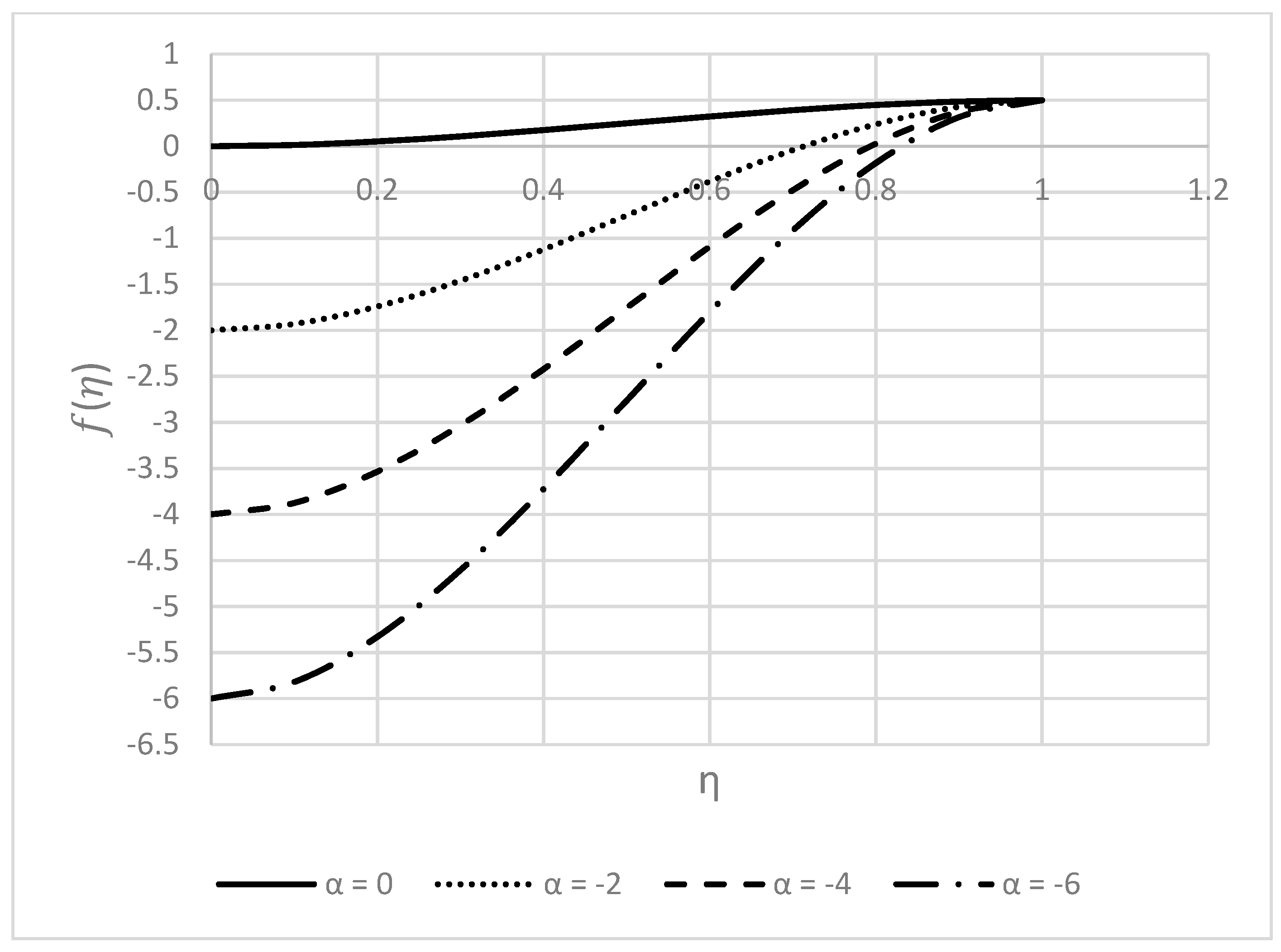Figure 3 represents the variation in the axial velocity for the above-mentioned fixed parameters. The axial velocity has increased behavior from the lower to the upper disk in the case of no suction. When the fluid starts moving out from the lower disk, the axial velocity has decreased behavior. Figure 3 also shows that the axial velocity increases upon increasing suction parameters.

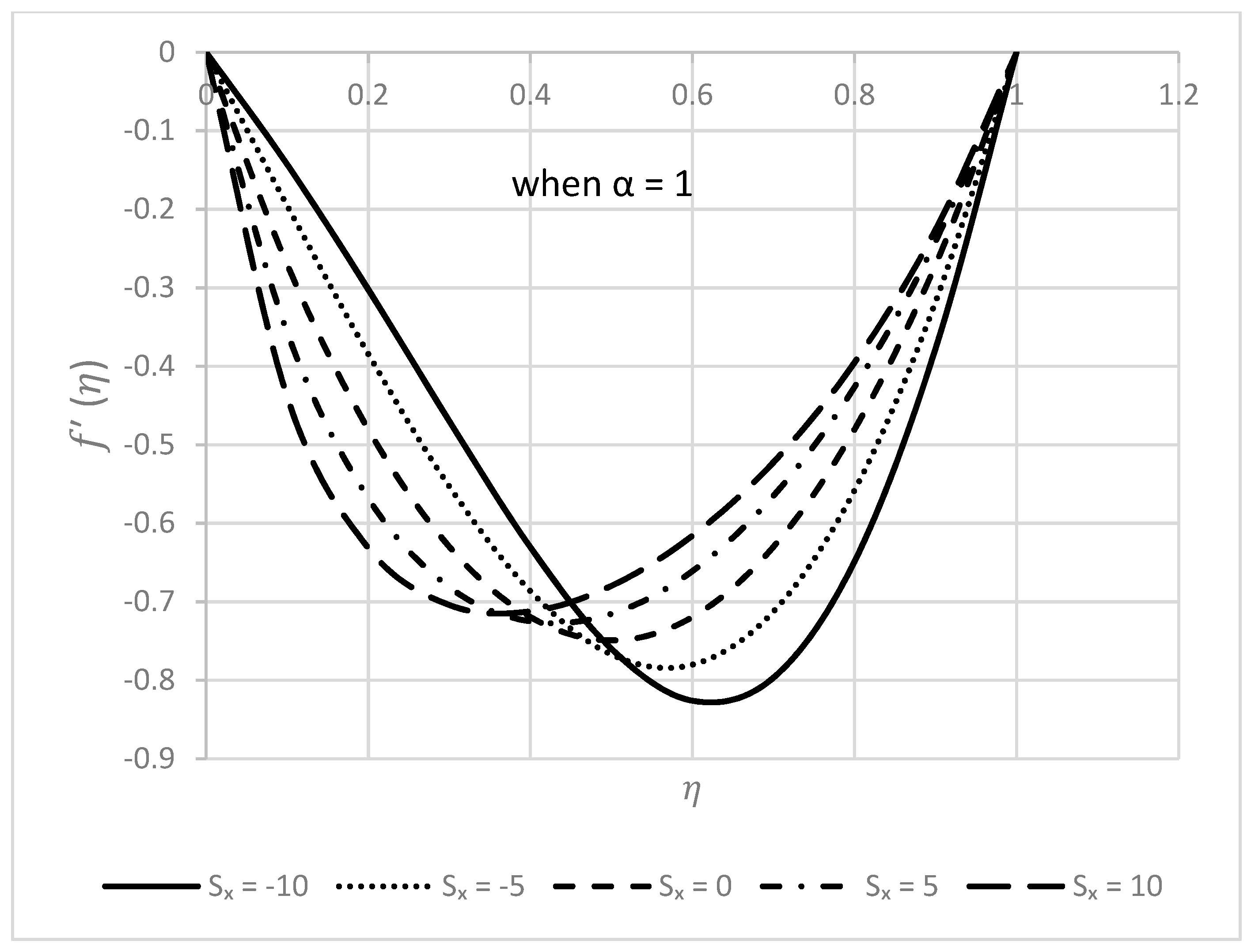
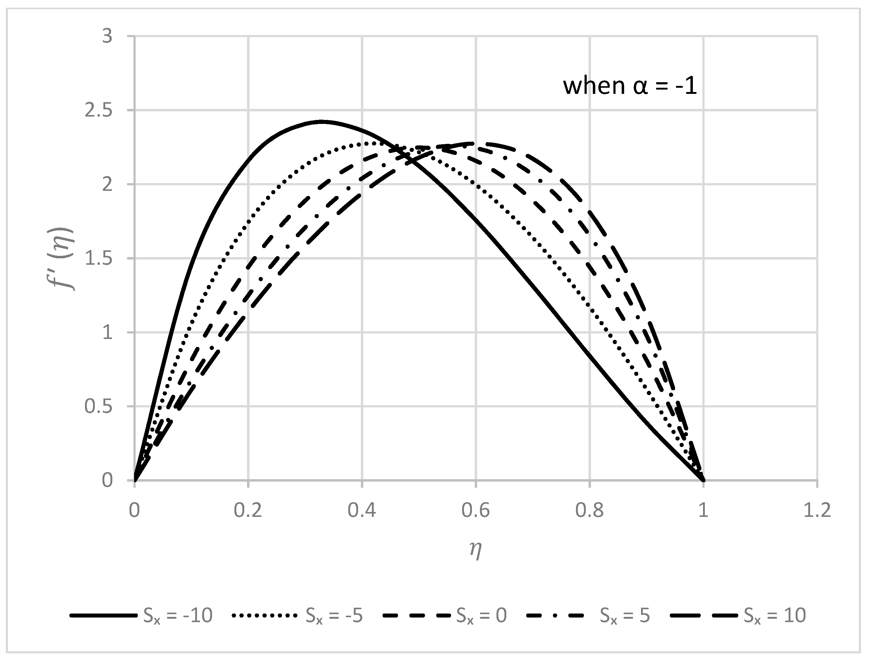
The effect of the squeezing parameter $\left(S_x\right)$ on both velocities is displayed in Figure 4 and Figure 5, when $H_a=1, \alpha =1, \varphi =0.05$, and ${\beta }_e=0.5$. $S_x$ is taken as negative when the upper disk is moving down, i.e., towards the lower disk, and positive values of $S_x$ describe the away motion of the upper disk. Figure 4 elucidates that the radial velocity falls from the lower disk and rises near the upper disk when the upper disk moves towards the fixed lower disk. Its behavior is symmetric when there is no movement, and when $S_x>0$, the velocity falls near the lower disk and increases thereafter. It can also be observed that minimum values of the radial velocity shift towards the lower disks as we increased the suction parameter. 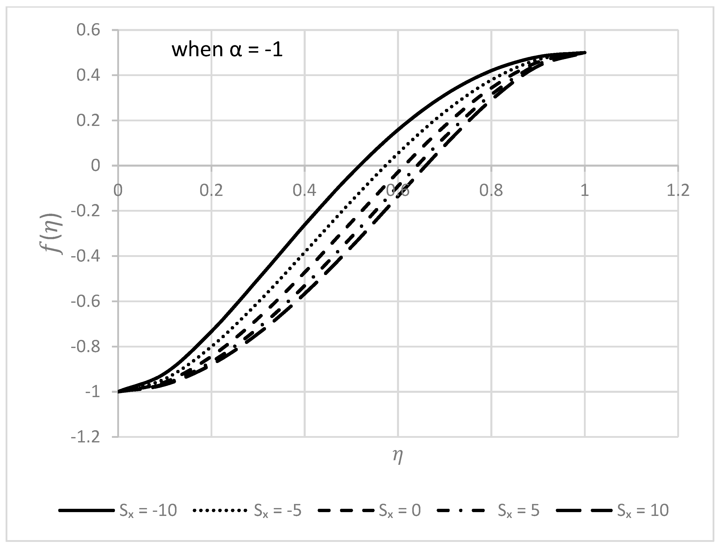The behavior of the axial velocity is shown in Figure 5. The axial velocity has decreased in nature in the entire gap length from the lower disk to the upper disk. It also decreases by increasing the suction parameter.

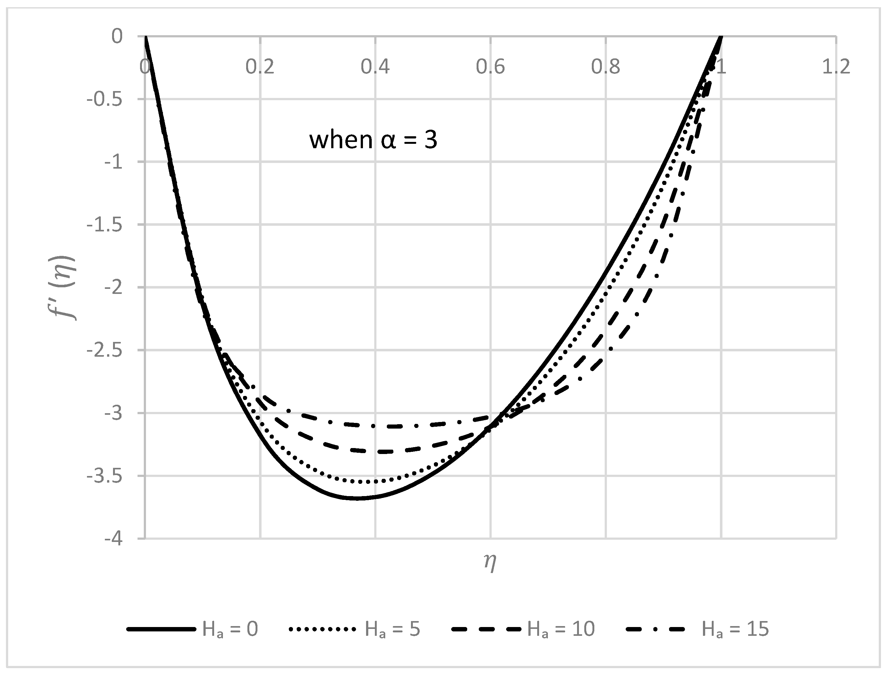
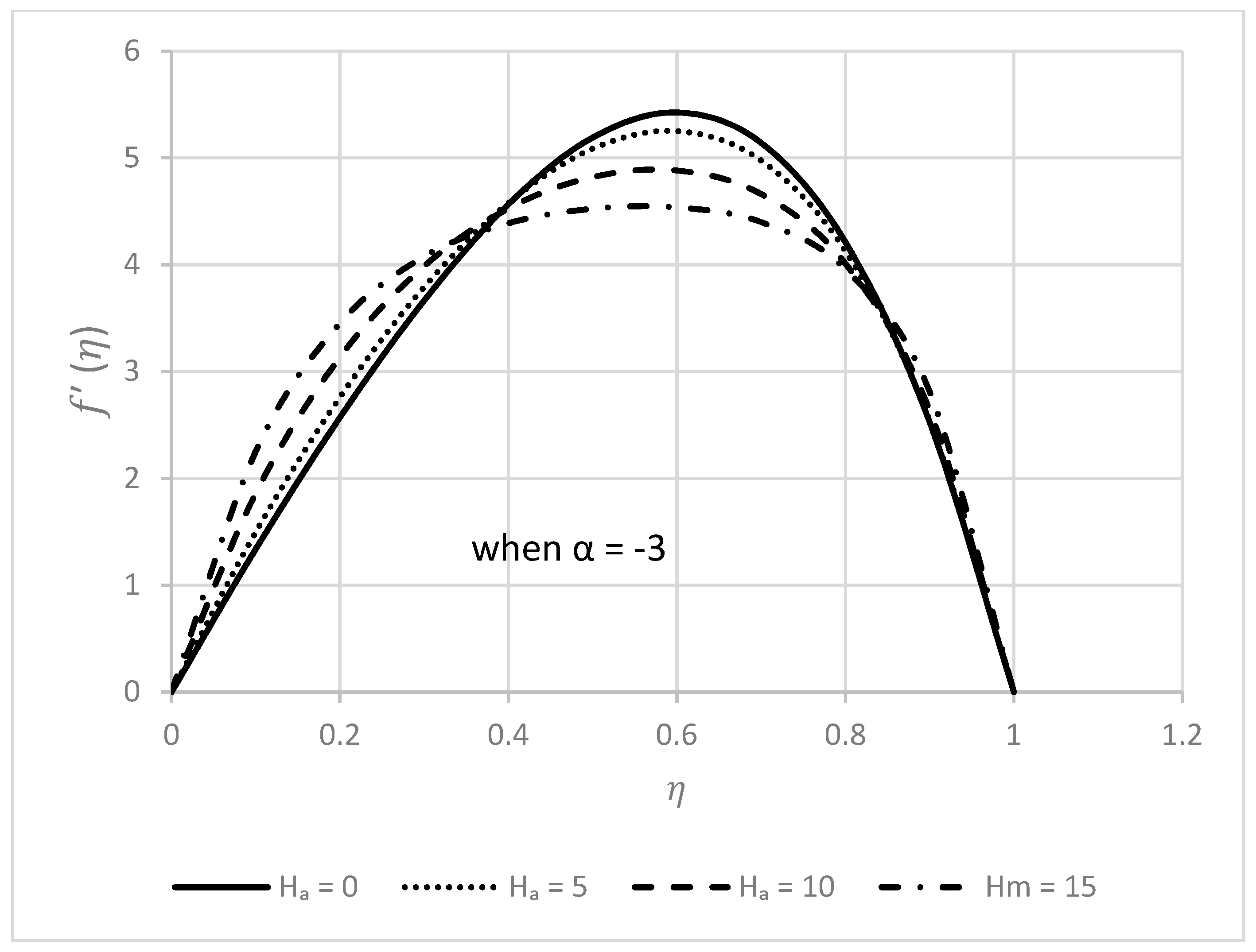
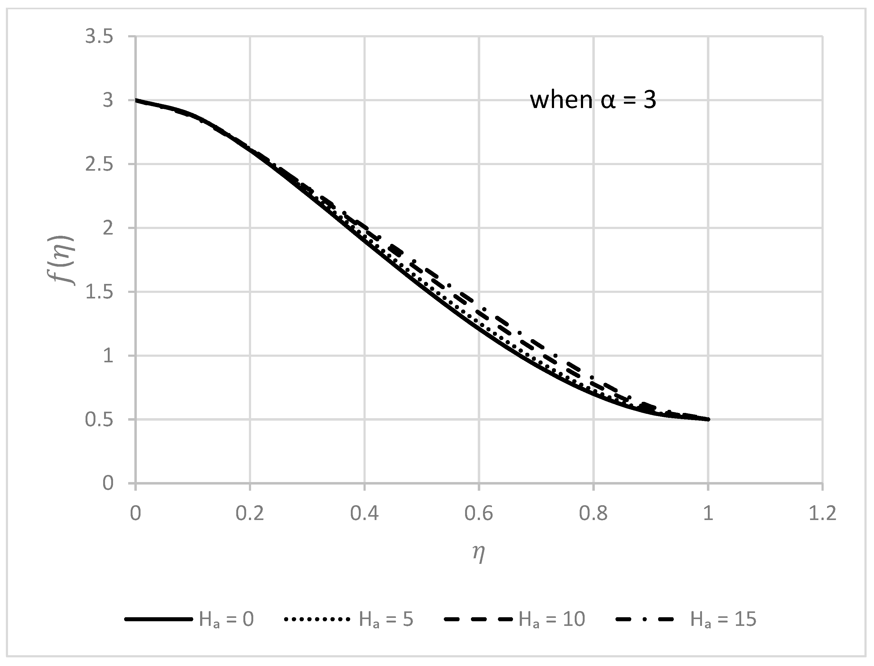
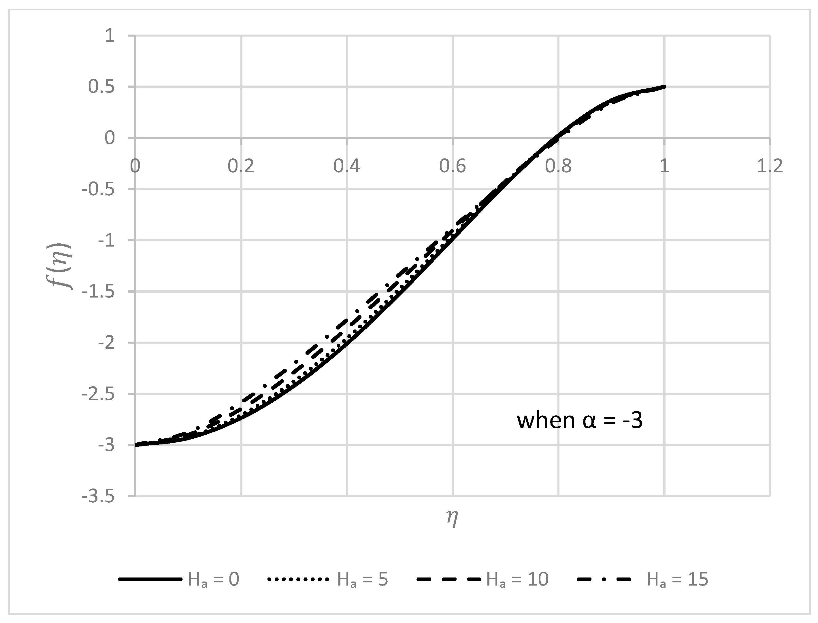
The impact of the Hartmann number $H_a$ on profiles is analyzed in Figure 6 and Figure 7. In this calculation, the other parameters are taken as $S_x=3, \alpha =3, \varphi =0.05$, and ${\beta }_e=0.5$. No significant effect can be observed in the much-closed region of the lower disk from Figure 6, but the radial velocity has increased behavior in the approximate middle of both disks. It is also significant to mention that the influence towards the upper disk is more impressive than the lower disk. The nature of the axial velocity can be easily studied from Figure 7. The axial velocity decreases throughout the region. It also expands with a rise in the values of the $H_a$ in the nearby middle.

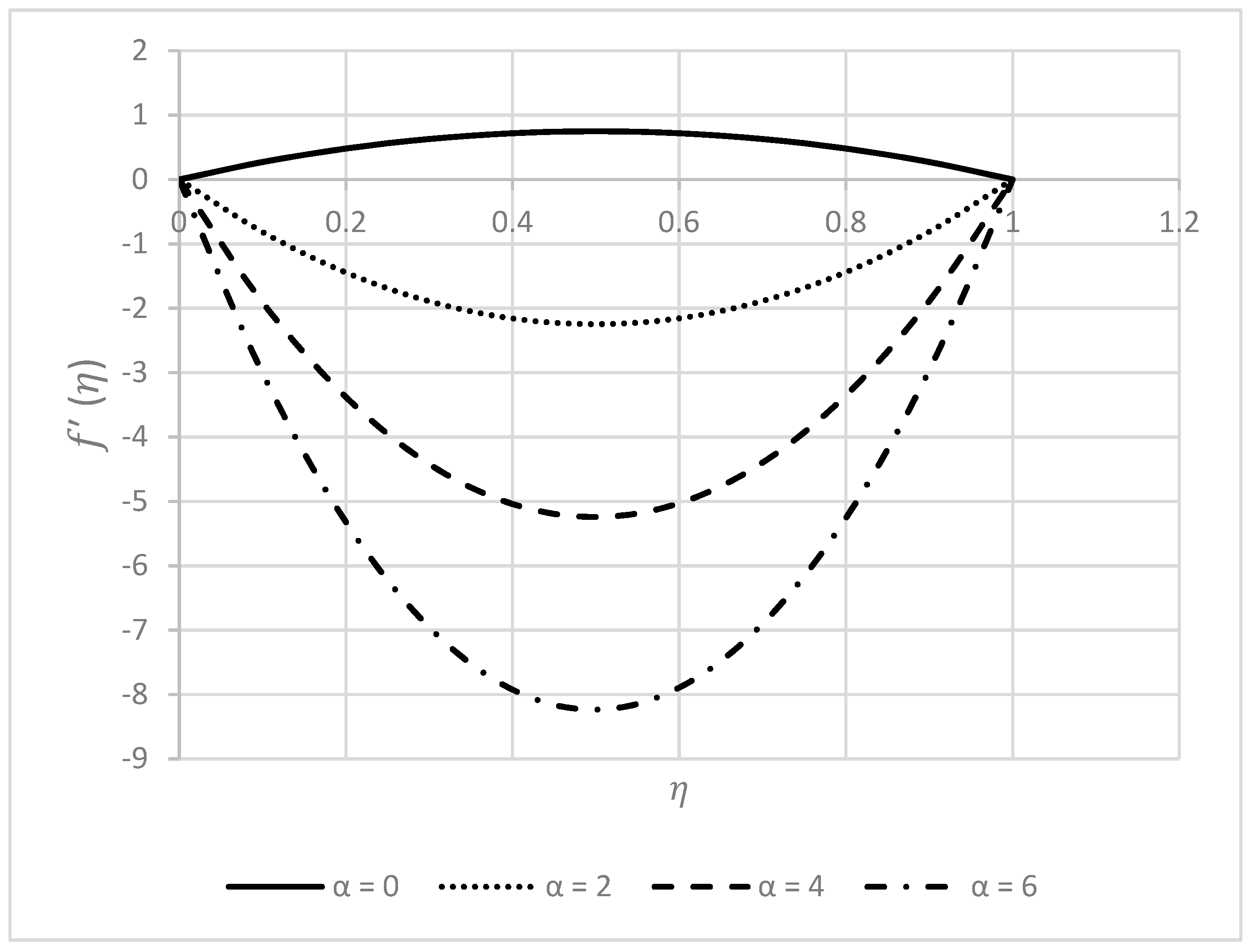
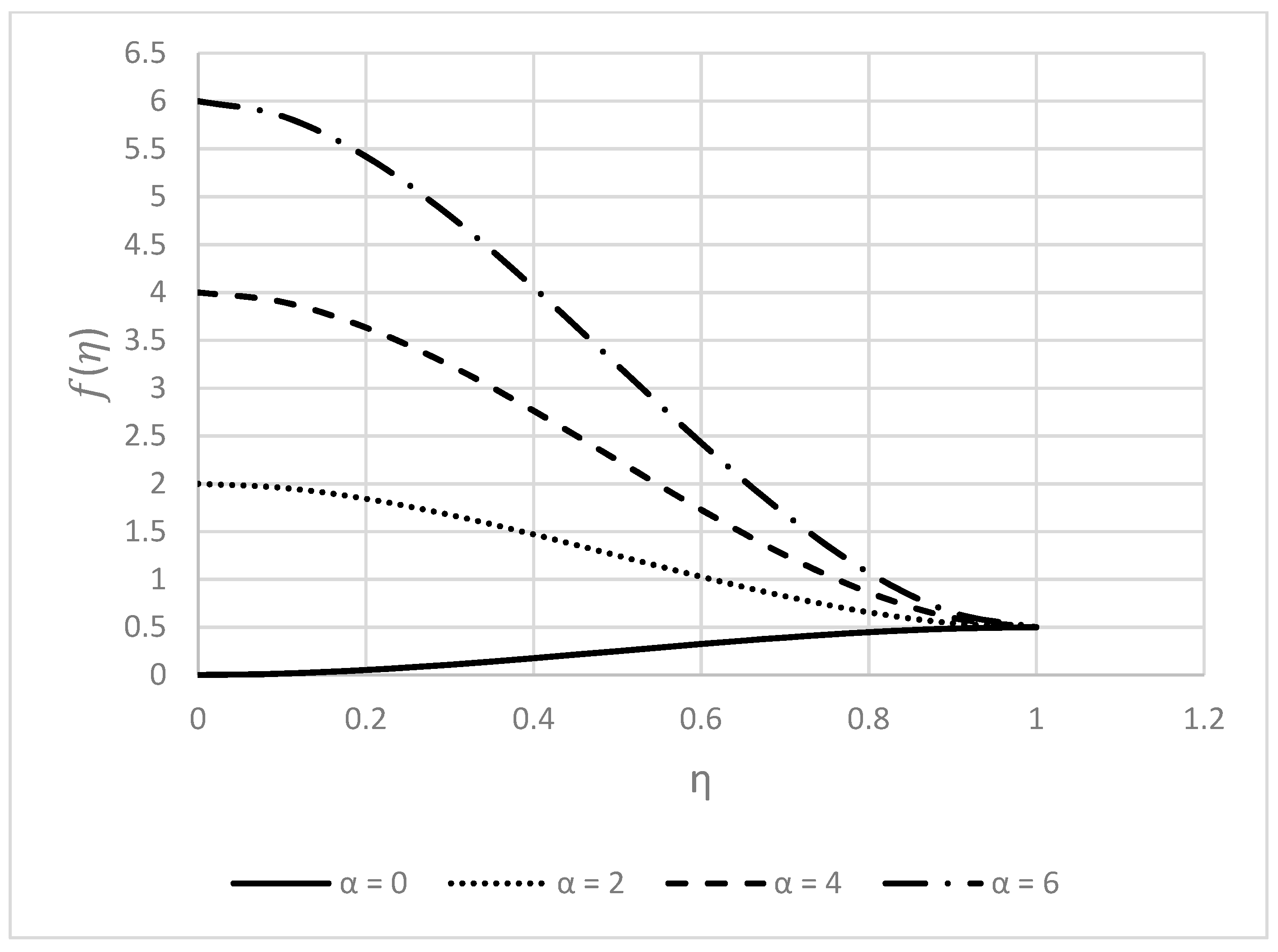
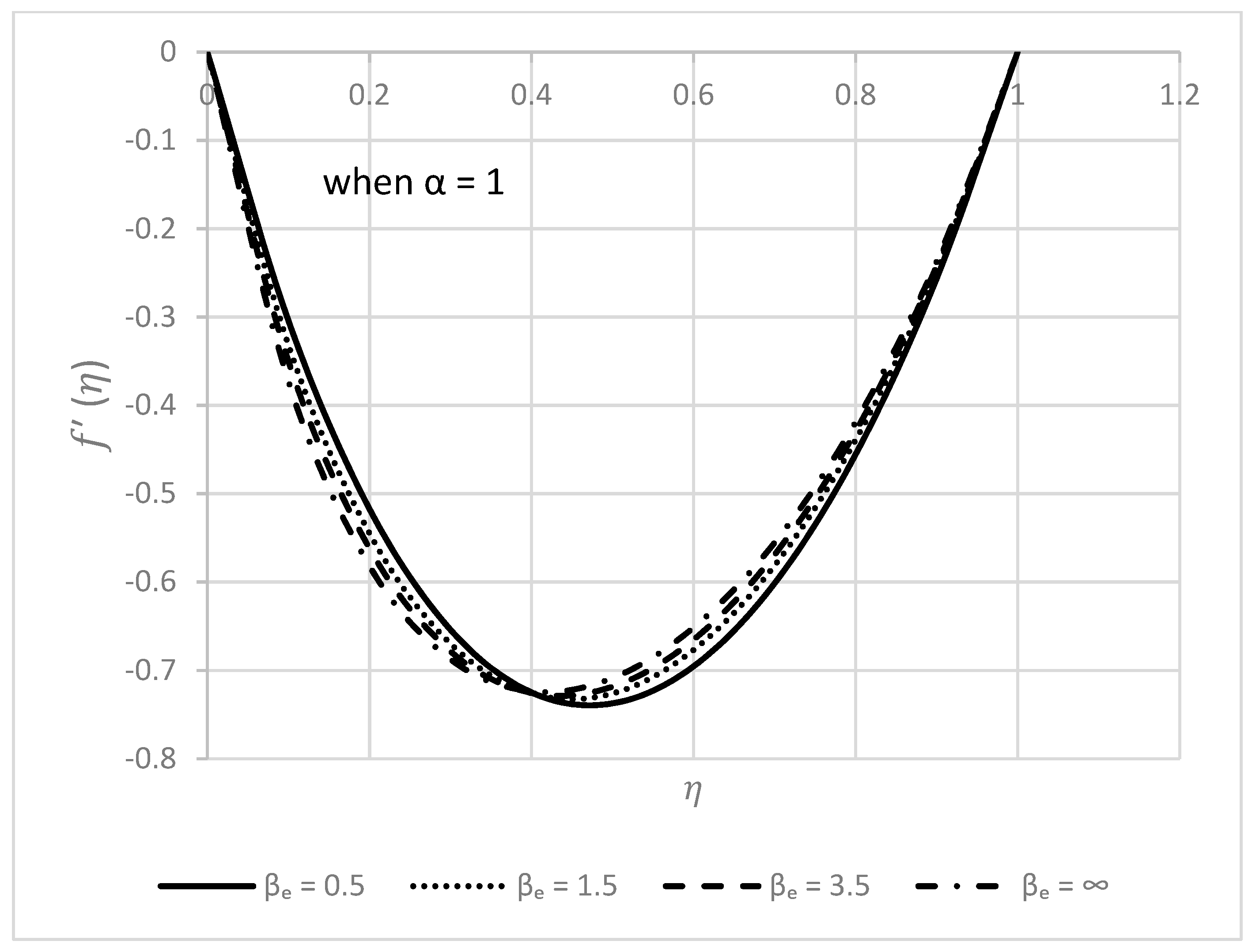
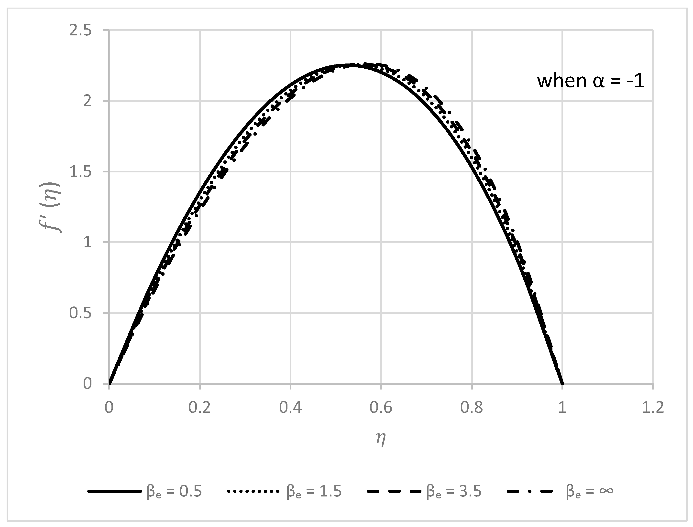
Figure 8 and Figure 9 are specially dedicated to the impact of the increasing Casson parameter ${\beta }_e$ on $f^{\prime }\left(\eta \right)$ and $f\left(\eta \right)$. Figure 8 demonstrates that as ${\beta }_e$ increases, the radial velocity near the lower disk drops. However, this tendency shifts to the contrary after traveling a certain distance from the lower disk; specifically, around $0.4$, we can see an accelerated radial flow. 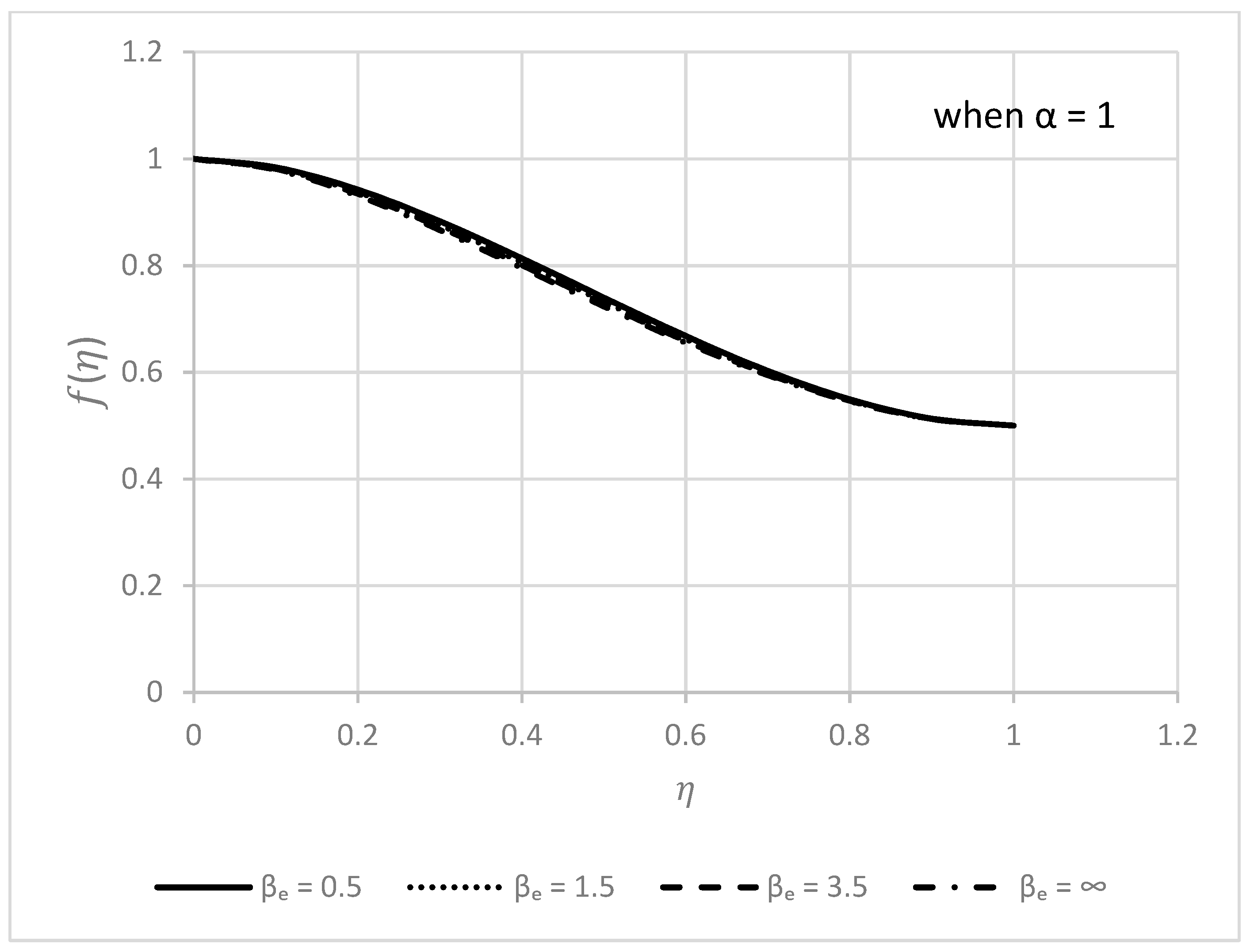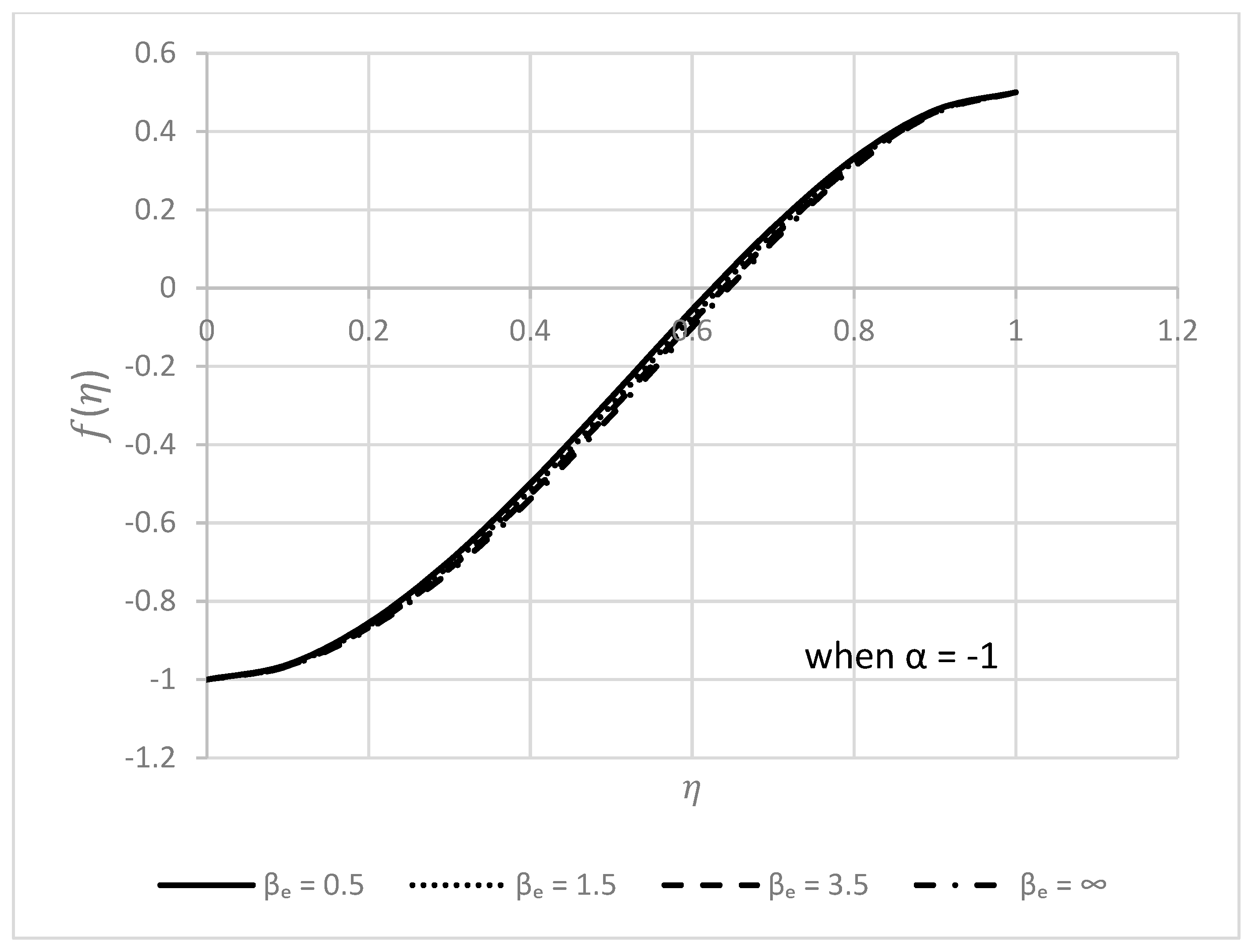Additionally, it may be seen that the impacts of ${\beta }_e$ are significantly less noticeable close to the disks than they are elsewhere. 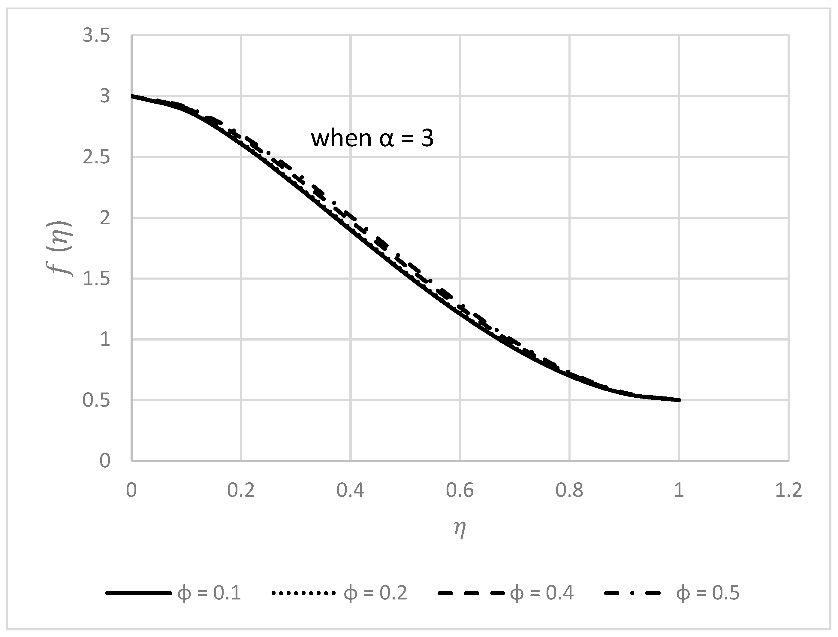According to Figure 9, the axial velocity has decreasing nature. A slight increment can be observed in the middle region, whereas near both disks, there is no convincing change in the values of the axial velocity.

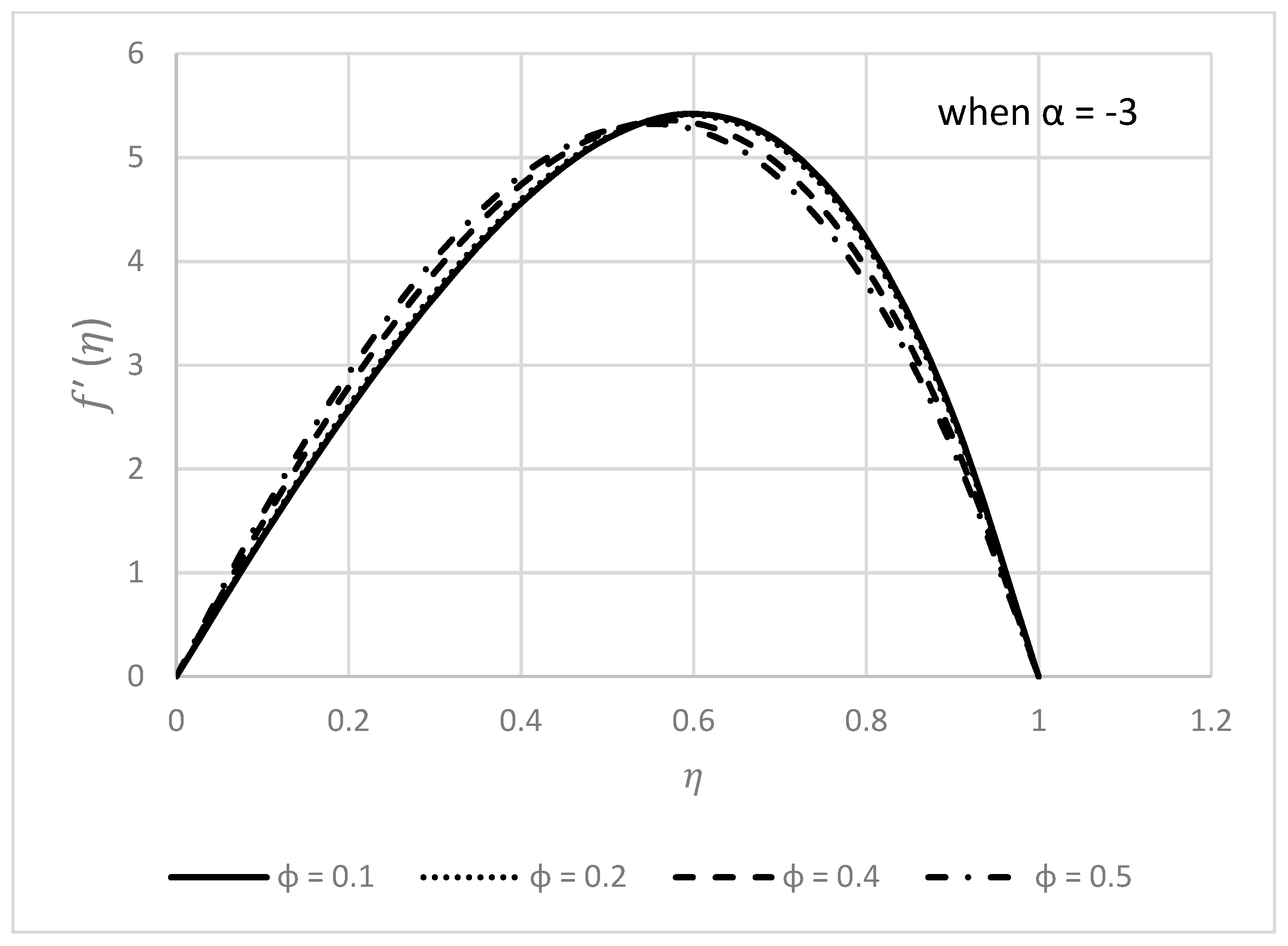
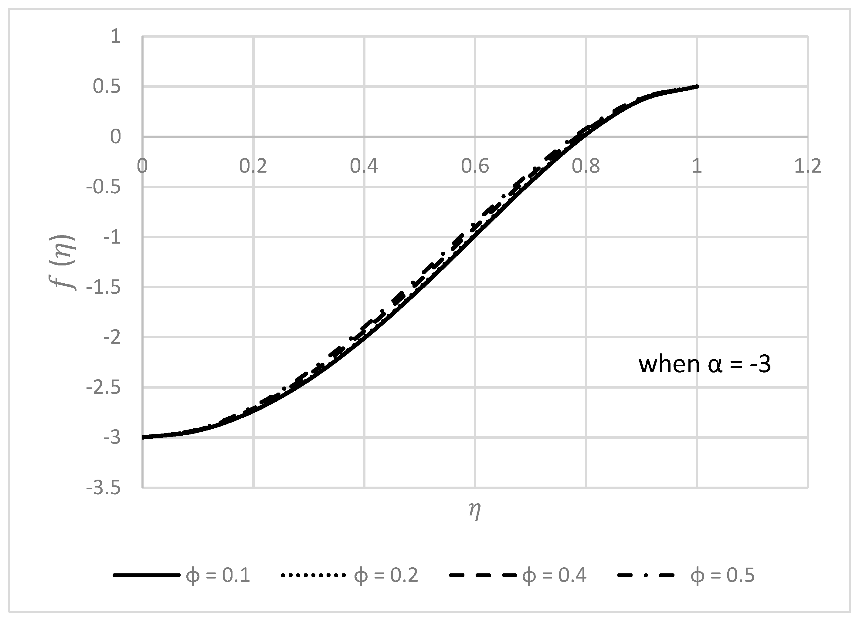
The nature of velocity profiles for different values of nanoparticle volume fraction $\left(\varphi \right)$ is presented in Figure 10 and Figure 11. Figure 10 presents a decreased nature of the radial velocity near the lower disk while increasing after crossing $\eta \approx 0.4$. On the other hand, velocity accelerates with increasing $\varphi$ but its nature turns to the opposite near the upper disk. Decreasing behavior can be seen in Figure 11. Moreover, axial velocity increased with rising values of $\varphi$.

5.2. Case of Injection When $\alpha$ Is Negative

This section is dedicated to the consequences of the above-discussed parameters on the velocity profiles in the case of injection, presented in Figure 12, Figure 13, Figure 14, Figure 15, Figure 16, Figure 17, Figure 18, Figure 19, Figure 20 and Figure 21. According to Figure 12 and Figure 13, increasing injection causes both velocities to increase in value. In all other figures (Figure 14, Figure 15, Figure 16, Figure 17, Figure 18, Figure 19, Figure 20 and Figure 21), the behaviors of velocity profiles in the injection case are completely contrary to those found in the suction condition.

6. Conclusions

The differential transform method successfully investigates the flowing nature of the Casson nanofluid. The results estimated by DTM and the outcomes of the numerical results are an exact match. The comparison analysis demonstrates the reliability and precision of DTM. It can be observed by the study that for all key variables, the flowing characteristics show opposite behavior in the case of suction and injection. The agreement between DTM and the numerical results of the skin friction coefficient and velocity profiles proves the novelty of this research.

References

- Stefen, M.J. Versuch Uber die scheinbare adhesion. Sitzungsberichte der Akademie der Wissenschaften in Wien. Mathematik-Naturwissen 1874, 69, 713–721. [Google Scholar]
- Leider, P.J.; Bird, R.B. Squeezing flow between parallel disks. I. Theoretical analysis. Ind. Eng. Chem. Fundam. 1974, 13, 336–341. [Google Scholar] [CrossRef]
- Qayyum, A.; Awais, M.; Alsaedi, A.; Hayat, T. Unsteady squeezing flow of Jeffery fluid between two parallel disks. Chin. Phys. Lett. 2012, 29, 034701. [Google Scholar] [CrossRef]
- Mohyud-Din, S.T.; Khan, S.I. Nonlinear radiation effects on squeezing flow of a Casson fluid between parallel disks. Aerosp. Sci. Technol. 2016, 48, 186–192. [Google Scholar] [CrossRef]
- Song, Y.Q.; Hamid, A.; Khan, M.I.; Gowda, R.P.; Kumar, R.N.; Prasannakumara, B.C.; Khan, S.U.; Khan, M.I. Solar energy aspects of gyrotactic mixed bioconvection flow of nanofluid past a vertical thin moving needle influenced by variable Prandtl number. Chaos Solitons Fractals 2021, 151, 111244. [Google Scholar] [CrossRef]
- Naveed, A.; Umar, K.; Sheikh, I.K.; Yang, X.J.; Zulfiqar, A.Z.; Syed, T.M.D. Magneto hydrodynamic (MHD) squeezing flow of a Casson fluid between parallel disks. Int. J. Phys. Sci. 2013, 8, 1788–1799. [Google Scholar]
- Hussain, T.; Xu, H. Time-dependent squeezing bio-thermal MHD convection flow of a micropolar nanofluid between two parallel disks with multiple slip effects. Case Stud. Therm. Eng. 2022, 31, 101850. [Google Scholar] [CrossRef]
- Khan, M.I.; Hayat, T.; Afzal, S.; Khan, M.I.; Alsaedi, A. Theoretical and numerical investigation of Carreau–Yasuda fluid flow subject to Soret and Dufour effects. Comput. Methods Programs Biomed. 2020, 186, 105145. [Google Scholar] [CrossRef]
- Choi, S.U.; Eastman, J.A. Enhancing Thermal Conductivity of Fluids with Nanoparticles; No. ANL/MSD/CP-84938; CONF-951135-29; Argonne National Lab. (ANL): Argonne, IL, USA, 1995. [Google Scholar]
- Eastman, J.A.; Choi, U.S.; Li, S.; Thompson, L.J.; Lee, S. Enhanced thermal conductivity through the development of nanofluids. MRS Online Proc. Libr. (OPL) 1996, 457, 3. [Google Scholar] [CrossRef]
- Xu, H.; Khan, S.I.U.; Ghani, U.; Bu, W.; Zeb, A. The Influence of Effective Prandtl Number Model on the Micropolar Squeezing Flow of Nanofluids between Parallel Disks. Processes 2022, 10, 1126. [Google Scholar] [CrossRef]
- Hashmi, M.M.; Hayat, T.; Alsaedi, A. On the analytic solutions for squeezing flow of nanofluid between parallel disks. Nonlinear Anal. Model. Control 2012, 17, 418–430. [Google Scholar] [CrossRef]
- Dinarvand, S.; Mousavi, S.M.; Yousefi, M.; Rostami, M.N. MHD flow of MgO-Ag/water hybrid nanofluid past a moving slim needle considering dual solutions: An applicable model for hot-wire anemometer analysis. Int. J. Numer. Methods Heat Fluid Flow 2021, 32, 488–510. [Google Scholar] [CrossRef]
- Hayat, T.; Abbas, T.; Ayub, M.; Muhammad, T.; Alsaedi, A. On the squeezed flow of Jeffrey nanofluid between two parallel disks. Appl. Sci. 2016, 6, 346. [Google Scholar] [CrossRef]
- Berrehal, H.; Dinarvand, S.; Khan, I. Mass-based hybrid nanofluid model for entropy generation analysis of flow upon a convectively warmed moving wedge. Chin. J. Phys. 2022, 77, 2603–2616. [Google Scholar] [CrossRef]
- Agarwal, R. Heat and mass transfer in electrically conducting micropolar fluid flow between two stretchable disks. Mater. Today Proc. 2021, 46, 10227–10238. [Google Scholar] [CrossRef]
- Agarwal, R.; Mishra, P.K. Analytical solution of the MHD forced flow and heat transfer of a non-Newtonian visco-inelastic fluid between two infinite rotating disks. Mater. Today Proc. 2021, 46, 10153–10163. [Google Scholar] [CrossRef]
- Agarwal, R. Analytical study of micropolar fluid flow between two porous disks. PalArch’s J. Archaeol. Egypt/Egyptol. 2020, 17, 903–924. [Google Scholar]
- Agarwal, R. An Analytical Study of Non-Newtonian Visco-inelastic Fluid Flow between two Stretchable Rotating disks. Palest. J. Math. 2022, 11, 184–201. [Google Scholar]
- Zhou, J.K. Differential Transformation and Its Applications for Electrical Circuits; Huazhong University Press: Wuhan, China, 1986. [Google Scholar]
- Usman, M.; Hamid, M.; Khan, U.; Din, S.T.M.; Iqbal, M.A.; Wang, W. Differential transform method for unsteady nanofluid flow and heat transfer. Alex. Eng. J. 2018, 57, 1867–1875. [Google Scholar] [CrossRef]
- Hatami, M.; Jing, D.; Yousif, M.A. Three-dimensional analysis of condensation nanofluid film on an inclined rotating disk by efficient analytical methods. Arab. J. Basic Appl. Sci. 2018, 25, 28–37. [Google Scholar] [CrossRef][Green Version]
- Sheikholeslami, M.; Ganji, D.D. Nanofluid flow and heat transfer between parallel plates considering Brownian motion using DTM. Comput. Methods Appl. Mech. Eng. 2015, 283, 651–663. [Google Scholar] [CrossRef]
Figure 1.
Structure of model.
Figure 2.
Behavior of for different (positive) values.
Figure 3.
Figure 4.
Behavior of for different values when .
Figure 5.
Figure 6.
Figure 7.
Figure 8.
Figure 9.
Figure 10.
Figure 11.
Figure 12.
Behavior of for different values.
Figure 13.
Figure 14.
Figure 15.
Figure 16.
Figure 17.
Figure 18.
Figure 19.
Figure 20.
Figure 21.