A Study of the Jacobi Stability of the Rosenzweig–MacArthur Predator–Prey System through the KCC Geometric Theory

Abstract

In this paper, we consider an autonomous two-dimensional ODE Kolmogorov-type system with three parameters, which is a particular system of the general predator–prey systems with a Holling type II. By reformulating this system as a set of two second-order differential equations, we investigate the nonlinear dynamics of the system from the Jacobi stability point of view using the Kosambi–Cartan–Chern (KCC) geometric theory. We then determine the nonlinear connection, the Berwald connection, and the five KCC invariants which express the intrinsic geometric properties of the system, including the deviation curvature tensor. Furthermore, we obtain the necessary and sufficient conditions for the parameters of the system in order to have the Jacobi stability near the equilibrium points, and we point these out on a few illustrative examples.

1. Introduction

M. Rosenzweig and R. MacArthur introduced in [1] a predator–prey system in order to understand the relationship between two populations, which involves the destruction of members of one population by members of another for the purpose of obtaining food. This system is a particular case of the predator–prey system of Holling’s type II [2,3].

The original Rosenzweig–MacArthur predator–prey system has the following form [1]:

$$\left\{\begin{array}{ccc}\hfill \dot{x}& =& rx\left(1-\frac{x}{K}\right)-y\frac{mx}{b+x}\hfill \\ \hfill \dot{y}& =& y\left(-\delta +c\frac{mx}{b+x}\right)\hfill \end{array}\right.$$

(1)

where the dot denotes the derivative with respect to time t, $x\ge 0$ denotes the prey density (#/unit of area) and $y\ge 0$ denotes the predator density (#/unit of area), the parameter $\delta >0$ is the death rate of the predator, the function $x\mapsto mx/(b+x)$ is the prey caught by the predator per unit of time, the function $x\mapsto rx/(1-x/K)$ is the growth of the prey in the absence of the predator (by the logistic growth model), and $c>0$ is the rate of the conversion from prey to predator.

The general case of the predator–prey systems with a Holling-type response function P is given by the following equation:

$$\left\{\begin{array}{ccc}\hfill \dot{x}& =& rx\left(1-\frac{x}{K}\right)-yP\left(x\right)\hfill \\ \hfill \dot{y}& =& y\left(-\delta +cP\left(x\right)\right)\hfill \end{array}\right.$$

(2)

with the same conditions on x, y and the parameters.

Depending of the expression of the function P, there are four types of predator–prey Holling-type systems, as demonstrated in the following [4]. If $P=mx$, then (2) is a predator–prey system of Holling’s type I. If $P=\frac{mx}{b+x}$, then (2) is a predator–prey system of Holling’s type II. In this case, the function $P=\frac{mx}{b+x}$ is an increasing function and tends to $m>0$ when $x\to \infty$, and P is often called a Michaelis–Menten function or a response function of Holling’s type II. If $P=\frac{m{x}^2}{a+x^2}$ or $P=\frac{m{x}^2}{a+bx+x^2}$, where a, b, m are strictly positive, then the function P is called a response function of Holling’s type III. If $P=\frac{mx}{a+x^2}$ or $P=\frac{mx}{a+bx+x^2}$, then the function P is called a response function of Holling’s type IV or a Monod–Haldane function. For more details about the predator–prey models (2) with Holling-type functional responses, see papers [4,5,6,7,8,9].

The predator–prey systems with response functions of the Holling type represent the mathematical models for the slow–fast dynamics in biology; more precisely, these are models where both the death rate and the conversion rate of prey to predator are kept very small [10].

In [11], R. Huzak reduced the study of the Rosenzweig–MacArthur system to study a polynomial differential system. In order to do that, the first step is to perform the following rescaling: $\left(\overline{x},\overline{y},\overline{b},\overline{c},\overline{\delta }\right)=\left(\frac{x}{K},\frac{m}{rK}y,\frac{b}{K},\frac{cm}{r},\frac{\delta }{r}\right)$. After once again denoting $\left(\overline{x},\overline{y},\overline{b},\overline{c},\overline{\delta }\right)$ by $\left(x,y,b,c,\delta \right)$ and then performing a time rescaling by multiplying it with $b+x$, the obtained polynomial differential system of the third degree is as follows:

$$\left\{\begin{array}{ccc}\hfill \dot{x}& =& x\left(-x^2-(1-b)x-y+b\right)\hfill \\ \hfill \dot{y}& =& y\left((c-\delta )x-\delta b\right)\hfill \end{array}\right.$$

(3)

where b, c, and $\delta$ are positive parameters.

Of course, the study of this system will only be performed in the positive quadrant of the plane where it has an ecological meaning [11,12].

System (3) is a particular case of the Kolmogorov-type system. These systems were proposed by Kolmogorov in [13] in the year 1936 as an extension of the Lotka–Volterra systems of arbitrary dimension and arbitrary degree.

The classical stability (linear or Lyapunov stability) of the Rosenzweig–MacArthur predator–prey system was completely studied in [11,12]. In this work, we will study another type of stability for this predator–prey system for the first time, namely the Jacobi stability.The Jacobi stability is a natural extension of the geometric stability of the geodesic flow, from a manifold with a Riemann metric or a Finsler metric to a manifold with no metric [14,15,16,17,18,19]. Practically, the Jacobi stability indicates the robustness of a dynamical system defined by a system of second-order differential equations (or SODE), where this robustness measures the lack of sensitivity and adaptation to both the modifications of the internal parameters of the system and the change in the external environment. By using the Kosambi–Cartan–Chern (KCC) theory, the local behavior of dynamical systems from the point of view of the Jacobi stability has recently been studied by several authors in [15,16,20,21,22,23,24,25,26,27]. Hence, the local dynamics of the system is investigated by using the geometric objects that correspond to the system of the second-order differential equations (SODE), which is the system obtained from the given first-order differential system [28,29,30].

The KCC theory deals with the study of the deviation of neighboring trajectories, which allows us to to estimate the perturbation permitted around the equilibrium points of the second-order differential system. Initially, this approach was linked with the study of the variation equations (or Jacobi field equations) associated with the geometry on the differentiable manifold. More exactly, P.L. Antonelli, R. Ingarden, and M. Matsumoto started the study of the Jacobi stability for the geodesics corresponding to a Riemannian or Finslerian metric by deviating the geodesics and using the KCC-covariant derivative for the differential system in variations [14,15,16]. As a result, the second KCC-invariant appeared, also called the deviation curvature tensor, which is essential for the establishment of the Jacobi stability for geodesics and generally for the trajectories associated with a system of second-order differential equations. In the theory of differential geometry, a system of second-order differential equations (SODE) is called semispray. Using a semispray, we can define a nonlinear connection on the manifold, and conversely, using a nonlinear connection, we can define a semispray. Consequently, any SODE can define a geometry on the manifold with the associated geometric objects, and the other way around [17,31,32,33]. Of course, these geometric objects are tensors that can check the properties of symmetry or not, depending on the particularity of the SODE.

The KCC theory originated from the works of D. D. Kosambi [28], E. Cartan [29], and S. S. Chern [30]; hence, the abbreviation KCC (Kosambi–Cartan–Chern). This geometric theory can be successfully applied in many research fields, from in engineering, physics, chemistry, and biology [20,23,25,26,27,34]. In addition, new approaches and results from the KCC theory in gravitation and cosmology were made in [35,36]. Moreover, in [22], a comprehensive analysis of the Jacobi stability and its relations with the Lyapunov stability for dynamical systems was made by C.G. Boehmer, T. Harko, and S.V. Sabau, who modeled the phenomena based on gravitation and astrophysics. Recently, in [37], a very interesting and complete study of the Jacobi stability for prey–predator models of Holling’s type II and III was performed.

In the second section, there will be a short presentation of the Rosenzweig–MacArthur predator–prey system, and we will point out the main results on the local stability of this system. Then, in the third section, we will present a brief review of the basic notions and main tools of the KCC theory that are necessary for analyzing the Jacobi stability of dynamical systems. More exactly, we will present the five invariants of the KCC theory and the definition of the Jacobi stability. In the fourth section, a reformulation of the Rosenzweig–MacArthur predator–prey system (3) as a system of second-order differential equations will be obtained, and the five geometrical invariants for this system will be computed. The obtained results for the Jacobi stability of this predator–prey system near the equilibrium points will be presented in section five. More precisely, we will find the necessary and sufficient conditions that would allow us to obtain the Jacobi stability of the system near the equilibrium points. Consequently, for these parameter values, it is not possible to have a chaotic behavior for the Rosenzweig–MacArthur predator–prey system. Furthermore, at the end of the fifth section, we will obtain the deviation equations near every equilibrium point as well as the curvature of the deviation vector, and then perform a comparative analysis of the Jacobi stability and the Lyapunov stability in order to compare these two approaches. Finally, a lot of very interesting examples will be presented in the sixth section and the conclusions in the seventh section. As usual in differential geometry, the sum over the crossed repeated indices is understood.

2. The Rosenzweig–MacArthur Predator–Prey System

Next, we will study the Rosenzweig–MacArthur system with the following form:

$$\left\{\begin{array}{ccc}\hfill \dot{x}& =& x\left(-x^2+(1-b)x-y+b\right)\hfill \\ \hfill \dot{y}& =& y\left((c-\delta )x-\delta b\right)\hfill \end{array}\right.$$

(4)

where b, c, $\delta >0$ and $x,y\ge 0$.

In order to find the equilibrium points of this system and following [1,11], by analyzing the system below:

$$\left\{\begin{array}{ccc}\hfill x\left(-x^2+(1-b)x-y+b\right)& =& 0\hfill \\ \hfill y\left((c-\delta )x-\delta b\right)& =& 0\hfill \end{array}\right.$$

we have at most three equilibria:

• $E_0(0,0)$ with eigenvalues ${\lambda }_1=b$, ${\lambda }_2=-\delta b$;
• $E_1(1,0)$ with eigenvalues ${\lambda }_1=-b-1$, ${\lambda }_2=-(b\delta +\delta -c)$;
• $E_2\left(\frac{b\delta }{c-\delta },\frac{-bc(b\delta +\delta -c)}{{\left(c-\delta \right)}^2}\right)$ with eigenvalues ${\lambda }_{1,2}=\frac{b}{2{\left(c-\delta \right)}^2}\left(A\pm \sqrt{\delta B}\right)$, where

  $$A=-\delta (b\delta +\delta -c+bc)$$

  and

  $$B=\delta {(b\delta +\delta -c+bc)}^2+4c{(c-\delta )}^2(b\delta +\delta -c).$$

Let us remark that the third equilibrium $E_2$ exists only if $c\ne \delta$ and $0<b\delta <c-\delta$. In this case, the corresponding eigenvalues satisfy

$${\lambda }_1+{\lambda }_2=\frac{bA}{{\left(c-\delta \right)}^2}\mathrm{and}{\lambda }_1{\lambda }_2=\frac{b^2}{4{\left(c-\delta \right)}^4}\left(A^2-\delta B\right).$$

Additionally, $A^2-\delta B=-4c\delta {(c-\delta )}^2(b\delta +\delta -c)>0$ whenever $E_2$ exists.

Note that if $b\delta =c-\delta$, then $E_2=E_1$.

The authors of [12] obtained the following table, which describes the type of the equilibria according to the values of the parameters b, c, and $\delta$.

Let us remark that if $A=0$, i.e., $b\delta +\delta -c=-bc$, then we have $B=-4b{c}^2{(c-\delta )}^2<0$. Furthermore, in the last case, a Hopf bifurcation can occur at the equilibrium $E_2$ because $B<0$ and $A=0$.

Even though the system has only two equations and three parameters, it is not so easy to obtain the behavior of the system near the equilibrium points because the system has no symmetry properties, and computations can be very difficult. However, in 2022, a deep study of the linear stability around the equilibrium points was performed by E. Diz-Pita, J. Llibre, and M. V. Otero-Espinar in the paper [12], where the following results about the existence of limit cycles and a Hopf bifurcation at $E_2$ were obtained:

Theorem 1.

(a) If $0<b\delta <c-\delta$ and $A>0$, then there exists at least one limit cycle surrounding equilibrium point $E_2$.

(b) The equilibrium $E_2$ of the Rosenzweig–MacArthur predator–prey system (4) undergoes a supercritical Hopf bifurcation at $b_0=\frac{c-\delta }{c+\delta }$ (i.e., $A=0$).

For $b>b_0$, system (4) has a unique stable limit cycle bifurcating from the equilibrium point $E_2$.

(c) If $0<b\delta <c-\delta$ and $A>0$, the limit cycle surrounding the equilibrium point $E_2$ is unique.

Consequently, based on this result, the unique limit cycle of system (4) appeared from the equilibrium point $E_2$ in a Hopf bifurcation.

Moreover, from the proof of this theorem (see [12]), the results show that the equilibrium point $E_2$ is a weak stable focus when $B<0$ and $A=0$.

However, for cases 4, 6, and 7 from Table 1, it was not proved whether limit cycles existed or not. Using the Bendixson–Dulac Theorem [12], it was established only for some of the subcases that there are no limit cycles.

Table 1. The equilibrium points in the closed positive quadrant.

Case	Conditions	Type of Equilibrium Points
1	$b\delta >c-\delta$	$E_0$ saddle, $E_1$ stable node
2	$b\delta =c-\delta$	$E_0$ saddle, $E_1$ saddle node
3	$0<b\delta <c-\delta$, $B\ge 0$, $A>0$	$E_0$ saddle, $E_1$ saddle point,
		$E_2$ unstable node
4	$0<b\delta <c-\delta$, $B\ge 0$, $A<0$	$E_0$ saddle, $E_1$ saddle point,
		$E_2$ stable node
5	$0<b\delta <c-\delta$, $B<0$, $A>0$	$E_0$ saddle, $E_1$ saddle point,
		$E_2$ unstable focus
6	$0<b\delta <c-\delta$, $B<0$, $A<0$	$E_0$ saddle, $E_1$ saddle point,
		$E_2$ stable focus
7	$0<b\delta <c-\delta$, $B<0$, $A=0$	$E_0$ saddle, $E_1$ saddle point,
		$E_2$ weak stable focus (center)

Proposition 1.

If $0<b\delta <c-\delta$, $A<0$ and $1+c<b+\delta +b\delta$, then the Rosenzweig–MacArthur system (4) does not have periodic orbits in the set $\{(x,y)\in {\mathbf{R}}^2\left|x,y\ge 0\right.\}$.

Finally, for cases 4, 6, and 7 from Table 1, the following conjecture was announced in [12] and for which only some numerical evidences have been claimed.

Conjecture 2.

If $0<b\delta <c-\delta$, $A<0$, and $1+c>b+\delta +b\delta$, then there are no limit cycles for the Rosenzweig–MacArthur predator–prey system (4).

In the next sections, we will focus only on the study of the Jacobi stability in order to clarify the behavior of the system and to confirm this conjecture.

3. Kosambi–Cartan–Chern (KCC) Geometric Theory and Jacobi Stability

Based on [26,27], in this section, we will make a brief presentation of the essential notions and principal results from the Kosambi–Cartan–Chern (KCC) theory [15,16,20,21,28,29,30]. Although the Kosambi–Cartan–Chern (KCC) theory is based on a classical approach of dynamical systems that use the geometric tools of differential geometry, the obtained results are totally new and very useful for the study of the behavior of dynamical systems. More exactly, with every SODE (or semispray), we can associate a nonlinear connection, a Berwald connection, and then the five geometrical invariants that determine the dynamics of the system: ${\epsilon }^i$—the external force, $P_j^i$—the deviation curvature tensor, $P_{jk}^i$—the torsion tensor, $P_{jkl}^i$—the Riemann–Christoffel curvature tensor, and $D_{jkl}^i$—the Douglas curvature tensor. However, fortunately, only the second invariant, the deviation curvature tensor $P_j^i$, determines the Jacobi stability of a dynamical system near an equilibrium point.

Next, we will introduce the main topics of the KCC theory following [14,15,16,20,21]. If we consider M a real, smooth n-dimensional manifold and $TM$ its tangent bundle, then $u=(x,y)$ is a point from $TM$, with $x=\left(x^1,\dots ,x^n\right)$, $y=\left(y^1,\dots ,y^n\right)$, and $y^i=\frac{d{x}^i}{dt}$, $i=1,\dots ,n$. Ordinarily, $M={\mathbf{R}}^n$ or M is an open subset of ${\mathbf{R}}^n$. Consider the following system of second-order differential equations in normalized form [14]:

$$\left\{\frac{d^2{x}^i}{d{t}^2}+2G^i(x,y)=0,i=1,\dots ,n.\right.$$

(5)

where $G^i(x,y)$ are smooth functions defined in a local system of coordinates on $TM$, usually an open neighborhood of some initial conditions $(x_0,y_0)$. System (5) can be viewed similarly to a system of Euler–Lagrange equations from classical dynamics [14,31], such as in the following equation:

$$\left\{\begin{array}{ccc}\hfill \frac{d}{dt}\frac{\partial L}{\partial y^i}-\frac{\partial L}{\partial x^i}& =& F^i\hfill \\ \hfill y^i& =& \frac{d{x}^i}{dt}\hfill \end{array}\right.,i=1,\dots ,n.$$

(6)

where $L(x,y)$ is a regular Lagrangian of $TM$, and $F^i$ represents the external forces.

System (5) has a geometrical meaning if and only if “the accelerations” $\frac{d^2{x}^i}{d{t}^2}$ and “the forces” $G^i(x^j,y^j)$ are $(0,1)$-type tensors under the following local coordinate transformation:

$$\left\{\begin{array}{ccc}\hfill {\tilde{x}}^i& =& {\tilde{x}}^i(x^1,\dots ,x^n)\hfill \\ \hfill {\tilde{y}}^i& =& \frac{\partial {\tilde{x}}^i}{\partial x^j}{y}^j\hfill \end{array}\right.,i=1,\dots ,n.$$

(7)

More precisely, System (5) has a geometrical meaning (and it is called a semispray ) if and only if the functions $G^i(x^j,y^j)$ are changing under the local coordinate transformation (7) following the rules below [14,31]:

$$2{\tilde{G}}^i=2G^j\frac{\partial {\tilde{x}}^i}{\partial x^j}-\frac{\partial {\tilde{y}}^i}{\partial x^j}{y}^j.$$

(8)

The basic idea of the KCC theory is to change the system of second-order differential equations (5) into an equivalent system (i.e., with the same solutions), but with geometrical meaning. Next, for this second-order system (SODE), we will define five tensor fields, also called geometric invariants of the KCC theory [15,16]. Of course, these are invariants under the local change coordinates (7). For this purpose, we will introduce the KCC-covariant differential of a vector field $\xi ={\xi }^i\frac{\partial }{\partial x^i}$ defined in an open set of $TM$ (usually $TM={\mathbf{R}}^n\times {\mathbf{R}}^n$) [15,28,29,30]:

$$\frac{D{\xi }^i}{dt}=\frac{d{\xi }^i}{dt}+N_j^i{\xi }^j,$$

(9)

where $N_j^i=\frac{\partial G^i}{\partial y^j}$ are the coefficients of a nonlinear connectionN on the tangent bundle $TM$ corresponding to the semispray (5).

For ${\xi }^i=y^i$, the following is obtained:

$$\frac{D{y}^i}{dt}=-2G^i+N_j^i{y}^j=-{\epsilon }^i.$$

(10)

The contravariant vector field ${\epsilon }^i$ is called the first invariant of the KCC theory. This invariant represents the external force, and the term ${\epsilon }^i$ has a geometrical character since with respect to coordinate transformation (7), we have the following [15]:

$${\tilde{\epsilon }}^i=\frac{\partial {\tilde{x}}^i}{\partial x^j}{\epsilon }^j.$$

If the functions $G^i$ are 2-homogeneous with respect to $y^i$, i.e., $\frac{\partial G^i}{\partial y^j}{y}^j=2G^i$, for all $i=1,\dots ,n$, then ${\epsilon }^i=0$ for all $i=1,\dots ,n$. Therefore, the first invariant of the KCC theory is null if and only if the semispray is a spray. This result is still available for the geodesic spray associated with a Riemann or Finsler metric [14,31].

The main objective of the Kosambi–Cartan–Chern theory is to study the trajectories which slightly deviate from a certain trajectory of (5). Practically, the dynamics of the system in variations will be studied, and then the trajectories $x^i\left(t\right)$ of (5) will be varied into nearby ones as described by the following equation:

$${\tilde{x}}^i\left(t\right)=x^i\left(t\right)+\eta {\xi }^i\left(t\right)$$

(11)

where $\left|\eta \right|$ is a small parameter, and ${\xi }^i\left(t\right)$ are the components of a contravariant vector field defined along the trajectories $x^i\left(t\right)$ and called the deviation vector. Hence, after substituting (11) into (5) and using the limit $\eta \to 0$, the next variational equations will be obtained [14,15,16]:

$$\frac{d^2{\xi }^i}{d{t}^2}+2N_j^i\frac{d{\xi }^j}{dt}+2\frac{\partial G^i}{\partial x^j}{\xi }^j=0$$

(12)

By using the KCC-covariant derivative from (9), Equation (12) can be written in the following covariant form [14,15,16]:

$$\frac{D^2{\xi }^i}{d{t}^2}=P_j^i{\xi }^j$$

(13)

where we have the $(1,1)$-type tensor $P_j^i$ on the right side with the following components:

$$P_j^i=-2\frac{\partial G^i}{\partial x^j}-2G^l{G}_{jl}^i+y^l\frac{\partial N_j^i}{\partial x^l}+N_l^i{N}_j^l.$$

(14)

According to [14,31], the coefficients

$$G_{jl}^i=\frac{\partial N_j^i}{\partial y^l}$$

(15)

represent the Berwald connection that is associated with the nonlinear connection N. If all coefficients of the nonlinear connection and the Berwald connection are identically zero, then the deviation curvature tensor from (14) becomes $P_j^i=-2\frac{\partial G^i}{\partial x^j}$.

Then, according to [34], we can introduce the so-called zero-connection curvature tensor Z given by the following equation:

$$Z_j^i=2\frac{\partial G^i}{\partial x^j}.$$

(16)

For two-dimensional systems, the zero-connection curvature Z corresponds to the Gaussian curvature K of the potential surface $V\left(x^i\right)=0$, where ${\dot{x}}^i=f^i\left(x^j\right)=-\frac{\partial V}{\partial x^i}\left(x^j\right)$. When the potential surface is minimal, then we have $P=-K$.

The coefficients $P_j^i$ represent the so-called deviation curvature tensor and is the second invariant of the Kosambi–Cartan–Chern theory. Equation (12) is called the deviation equations (or Jacobi equations), and the invariant Equation (13) is also called the Jacobi equations. In Riemannian or Finslerian geometry, when the second-order system of equations represents the geodesic motion, then Equation (12) (or even (13)) is exactly the Jacobi field equation corresponding to the given geometry.

Finally, we can introduce the third, the fourth, and the fifth invariants of the Kosambi–Cartan–Chern (KCC) theory for the second-order system of Equation (5). These invariants are defined by the following:

$$\begin{array}{c}{P}_{jk}^i=\frac{1}{3}\left(\frac{\partial P_j^i}{\partial y^k}-\frac{\partial P_k^i}{\partial y^j}\right),\\ \\ P_{jkl}^i=\frac{\partial P_{jk}^i}{\partial y^l},D_{jkl}^i=\frac{\partial G_{jk}^i}{\partial y^l}.\end{array}$$

(17)

From the geometrical point of view, the third KCC invariant $P_{jk}^i$ can be interpreted as a torsion tensor. The fourth and the fifth KCC invariants $P_{jkl}^i$ and $D_{jkl}^i$ represent the Riemann–Christoffel curvature tensor and the Douglas tensor, respectively.

It is important to point out that these tensors always exist [14,15,16,21,31].

According to [14,29,31], these five invariants are the basic mathematical quantities that describe the geometrical properties of the system and give us the geometrical interpretation for an arbitrary system of second-order differential equations.

Next, we present a basic result of the KCC theory, which was obtained by P.L. Antonelli in [15]:

Theorem 3.

Two second-order differential systems of the same type as (5), such as

$$\frac{d^2{x}^i}{d{t}^2}+2G^i(x^j,y^j)=0,y^j=\frac{d{x}^j}{dt}$$

and

$$\frac{d^2{\tilde{x}}^i}{d{t}^2}+2{\tilde{G}}^i({\tilde{x}}^j,{\tilde{y}}^j)=0,{\tilde{y}}^j=\frac{d{\tilde{x}}^j}{dt}$$

can be locally transformed, from one into another, via changing coordinate transformation (7) if and only if the five invariants ${\epsilon }^i$, $P_j^i$, $P_{jk}^i$, $P_{jkl}^i$, and $D_{jkl}^i$ are equivalent tensors of ${\tilde{\epsilon }}^i$, ${\tilde{P}}_j^i$, ${\tilde{P}}_{jk}^i$, ${\tilde{P}}_{jkl}^i$, and ${\tilde{D}}_{jkl}^i$, respectively.

More specifically, there are local coordinates $(x^1,\dots ,x^n)$ on the manifold M, for which $G^i=0$ for all i, if and only if all five invariant tensors are null. In this particular case, the trajectories of the dynamical systems are straight lines.

The term “Jacobi stability” in the Kosambi–Cartan–Chern theory comes from the fact that when (5) represents the system of second-order differential equations for the geodesics in Riemannian or Finslerian geometry, then Equation (13) is exactly the Jacobi field equation for the geodesic deviation. More generally, we can write the Jacobi Equation (13) of the Finslerian manifold $(M,F)$ in the following scalar form [18]:

$$\frac{d^{2}v}{d{s}^2}+K·v=0$$

(18)

where ${\xi }^i=v\left(s\right){\eta }^i$ is the Jacobi field along the geodesic $\gamma :x^i=x^i\left(s\right)$, ${\eta }^i$ is the unit normal vector field on the geodesic $\gamma$, and K is the flag curvature associated with the Finslerian F.

Moreover, regarding the sign of the flag curvature K, it can be said that: if $K>0$, then the geodesics bunch together (i.e., are Jacobi-stable), and if $K<0$, then the geodesics disperse (i.e., are Jacobi-unstable). Therefore, from the equivalence of (13) and (18), we obtain that a positive flag curvature is equivalent to the negative eigenvalues of the curvature deviation tensor $P_j^i$, and a negative flag curvature is equivalent to positive eigenvalues. Then, we have a well-known result from the Kosambi–Cartan–Chern theory [22]:

Theorem 4.

The trajectories of system (5) are Jacobi-stable if and only if the real parts of the eigenvalues of the deviation tensor $P_j^i$ are strictly negative everywhere; otherwise, they are Jacobi-unstable.

Next, according to the definition of the Jacobi stability for a geodesic associated with a Euclidean, Riemannian, or Finslerian metric [19], there can be a rigorous definition for the Jacobi stability of a trajectory $x^i=x^i\left(s\right)$ of the dynamical system corresponding to (5) [20,21,22]:

Definition 1.

A trajectory $x^i=x^i\left(s\right)$ of (5) is called Jacobi-stable if for any $\epsilon >0$, there exists $\delta \left(\epsilon \right)>0$, such that $\parallel {\tilde{x}}^i\left(s\right)-x^i\left(s\right)\parallel <\epsilon$ for all $s\ge s_0$ and for all trajectories ${\tilde{x}}^i={\tilde{x}}^i\left(s\right)$, with $\parallel {\tilde{x}}^i\left(s_0\right)-x^i\left(s_0\right)\parallel <\delta \left(\epsilon \right)$ and $\parallel \frac{d{\tilde{x}}^i}{ds}\left(s_0\right)-\frac{d{x}^i}{ds}\left(s_0\right)\parallel <\delta \left(\epsilon \right)$.

According with [19,20,21,22], we consider the trajectories of system (5) as curves in a Euclidean space ${\mathbf{R}}^n$, where the norm $\parallel ·\parallel$ is the norm induced by the canonical inner product $<·,·>$ on ${\mathbf{R}}^n$. Moreover, we will suppose that the deviation vector $\xi$ from (13) verifies the initial conditions $\xi \left(s_0\right)=O$ and $\dot{\xi }\left(s_0\right)=W\ne O$, where O is the null vector from ${\mathbf{R}}^n$. Additionally, if we assume that $s_0=0$ and $\parallel W\parallel =1$, then for $s\searrow 0$, the trajectories of system (5) merge together if and only if the real parts of all eigenvalues of $P_j^i\left(0\right)$ are strictly negative, or the trajectories of system (5) disperse if and only if at least one of the real parts of the eigenvalues of $P_j^i\left(0\right)$ is strictly positive.

The Jacobi’s type of stability is about focusing the tendency on a neighborhood that is small enough, such as $s_0=0$ of the trajectories of system (5), in relation to the variation of the trajectories in (11) that satisfy the conditions $\parallel {\tilde{x}}^i\left(0\right)-x^i\left(0\right)\parallel =0$ and $\parallel \frac{d{\tilde{x}}^i}{ds}\left(0\right)-\frac{d{x}^i}{ds}\left(0\right)\parallel \ne 0$.

We can point out that the system of second-order differential equations (SODE) (5) is Jacobi-stable if and only if the system in variations (12) is stable in the Lyapunov sense or is linear-stable. Consequently, the study of Jacobi stability is based on the study of the Lyapunov stability of all trajectories in a region, but without taking velocity into account. Therefore, even when there is reduction at an equilibrium point, this theory offers us information about the behavior of the trajectories in an open region around this equilibrium point.

4. SODE Formulation of the Rosenzweig–MacArthur Predator–Prey System

We consider the Rosenzweig–MacArthur predator–prey system (4). By taking the derivative with respect to time t in both equations of this system, we obtain the following equation:

$$\left\{\begin{array}{ccc}\ddot{x}+3x^2\dot{x}-2\left(1-b\right)x\dot{x}-\left(b-y\right)\dot{x}+x\dot{y}\hfill & =& \hfill 0\\ \ddot{y}-\left((c-\delta )x-\delta b\right)\dot{y}-y(c-\delta )\dot{x}\hfill & =& \hfill 0\end{array}\right.$$

If we change the notations of variables as follows:

$$x=x^1,\dot{x}=y^1,y=x^2,\dot{y}=y^2$$

then this system of second-order differential equations (SODEs) becomes

$$\left\{\begin{array}{ccc}{\ddot{x}}^1+3{\left(x^1\right)}^2{y}^1+2\left(b-1\right)x^1{y}^1+\left(x^2-b\right)y^1+x^1{y}^2\hfill & =& \hfill 0\\ {\ddot{x}}^2+\left(\delta b-(c-\delta )x^1\right)y^2-(c-\delta )x^2{y}^1\hfill & =& \hfill 0\end{array}\right.$$

(19)

or, equivalently,

$$\left\{\begin{array}{ccc}\frac{d^2{x}^1}{d{t}^2}+3{\left(x^1\right)}^2{y}^1+2\left(b-1\right)x^1{y}^1+\left(x^2-b\right)y^1+x^1{y}^2\hfill & =& \hfill 0\\ \frac{d^2{x}^2}{d{t}^2}+\left(\delta b-(c-\delta )x^1\right)y^2-(c-\delta )x^2{y}^1\hfill & =& \hfill 0\end{array}\right.$$

(20)

where $\frac{d{x}^i}{dt}=y^i$, $i=1,2$.

This system can be written similarly to SODEs from the KCC theory:

$$\left\{\begin{array}{c}\frac{d^2{x}^1}{d{t}^2}+2G^1(x^1,x^2,y^1,y^2)=0\\ \frac{d^2{x}^2}{d{t}^2}+2G^2(x^1,x^2,y^1,y^2)=0\end{array}\right.$$

(21)

where $\frac{d{x}^i}{dt}=y^i$, $i=1,2$, and

$$\begin{array}{ccc}{G}^1(x^i,y^i)\hfill & =& \frac{1}{2}\left[3{\left(x^1\right)}^2{y}^1+2\left(b-1\right)x^1{y}^1+\left(x^2-b\right)y^1+x^1{y}^2\right]\hfill \\ G^2(x^i,y^i)\hfill & =& \frac{1}{2}\left[\left(\delta -c\right)\left(x^1{y}^2+x^2{y}^1\right)+\delta b{y}^2\right]\hfill \end{array}$$

(22)

The zero-connection curvature $Z_j^i=2\frac{\partial G^i}{\partial x^j}$ has the following coefficients:

$$\begin{array}{ccc}\hfill Z_1^1& =& 6x^1{y}^1+2(b-1)y^1+y^2\hfill \\ \hfill Z_2^1& =& y^1\hfill \\ \hfill Z_1^2& =& (\delta -c)y^2\hfill \\ \hfill Z_2^2& =& (\delta -c)y^1\hfill \end{array}$$

Since $N_j^i=\frac{\partial G^i}{\partial y^j}$, the nonlinear connection N is given by the following coefficients:

$$\left\{\begin{array}{ccc}\hfill N_1^1& =& \frac{\partial G^1}{\partial y^1}=\frac{1}{2}\left[3{\left(x^1\right)}^2+2\left(b-1\right)x^1+x^2-b\right]\hfill \\ \hfill N_2^1& =& \frac{\partial G^1}{\partial y^2}=\frac{1}{2}{x}^1\hfill \\ \hfill N_1^2& =& \frac{\partial G^2}{\partial y^1}=\frac{1}{2}\left(\delta -c\right)x^2\hfill \\ \hfill N_2^2& =& \frac{\partial G^2}{\partial y^2}=\frac{1}{2}\left[\left(\delta -c\right)x^1+\delta b\right]\hfill \end{array}\right.$$

(23)

Then, all the resulting coefficients of the Berwald connection $G_{jk}^i=\frac{\partial N_j^i}{\partial y^k}$ are null.

The first invariant of the KCC theory ${\epsilon }^i=-\left(N_j^i{y}^j-2G^i\right)$ has the following components:

$$\left\{\begin{array}{ccc}\hfill {\epsilon }^1& =& \frac{3}{2}{\left(x^1\right)}^2{y}^1+\left(b-1\right)x^1{y}^1+\frac{1}{2}\left(x^2-b\right)y^1+\frac{1}{2}{x}^1{y}^2\hfill \\ \hfill {\epsilon }^2& =& \frac{1}{2}\left(\delta -c\right)\left(x^1{y}^2+x^2{y}^1\right)+\frac{1}{2}\delta b{y}^2\hfill \end{array}\right.$$

(24)

Let us remark that ${\epsilon }^i=G^i$ for $i=1,2$, which means that $\frac{\partial G^i}{\partial y^j}{y}^j=1·G^i$ for $i=1,2$, or equivalently, that the functions $G^i$ are 1-homogeneous with respect to $y^i$.

Next, taking (14) into account, we obtain the components of the second invariant of the KCC theory, which means that the deviation curvature tensor of the Rosenzweig–MacArthur system (4) is as follows:

$$\begin{array}{ccc}\hfill P_1^1& =& -3x^1{y}^1-(b-1)y^1-\frac{1}{2}{y}^2+\frac{1}{4}{\left[3{\left(x^1\right)}^2+2\left(b-1\right)x^1+x^2-b\right]}^2\hfill \\ \hfill & +& \frac{1}{4}(\delta -c)x^1{x}^2\hfill \\ \hfill P_2^1& =& -\frac{1}{2}{y}^1+\frac{1}{4}\left[3{\left(x^1\right)}^3+2\left(b-1\right){\left(x^1\right)}^2+(x^2-b)x^1+(\delta -c){\left(x^1\right)}^2+\delta b{x}^1\right]\hfill \\ \hfill P_1^2& =& -\frac{1}{2}(\delta -c)y^2+\frac{1}{4}(\delta -c)x^2·\left[3{\left(x^1\right)}^2+2\left(b-1\right)x^1+x^2-b\right.\hfill \\ \hfill & +& \left.(\delta -c)x^1+\delta b\right]\hfill \\ \hfill P_2^2& =& -\frac{1}{2}(\delta -c)y^1+\frac{1}{4}(\delta -c)x^1{x}^2+\frac{1}{4}{\left[(\delta -c)x^1+\delta b\right]}^2\hfill \end{array}$$

(25)

Then, the trace and the determinant of the following deviation curvature matrix:

$$P=\left(\begin{array}{cc}{P}_1^1& P_2^1\\ P_1^2& P_2^2\end{array}\right)$$

are trace$\left(P\right)=P_1^1+P_2^2$ and det$\left(P\right)=P_1^1{P}_2^2-P_1^2{P}_2^1$.

Therefore, following the results from the previous section, we have:

Theorem 5.

All the roots of the characteristic polynomial of P are negative or have negative real parts (i.e., Jacobi stability) if and only if

$$P_1^1+P_2^2<0and{P}_1^1{P}_2^2-P_1^2{P}_2^1>0.$$

Taking into account that $P_{jk}^i=\frac{1}{3}\left(\frac{\partial P_j^i}{\partial y^k}-\frac{\partial P_k^i}{\partial y^j}\right)$, $P_{jkl}^i=\frac{\partial P_{jk}^i}{\partial y^l}$, $D_{jkl}^i=\frac{\partial G_{jk}^i}{\partial y^l}$, we obtained the third, fourth, and fifth invariants of the Rosenzweig–MacArthur predator–prey system as follows:

Theorem 6.

The third KCC invariant $P_{jk}^i$, called the torsion tensor, has all eight components null, i.e.,

$$P_{jk}^i=0foralli,j,k.$$

(26)

The fourth KCC invariant $P_{jkl}^i$, called the Riemann–Christoffel curvature tensor, has all sixteen components null, i.e.,

$$P_{jkl}^i=0foralli,j,k,l.$$

(27)

The fifth KCC invariant $D_{jkl}^i$, called the Douglas tensor, has all sixteen components null, which means that

$$D_{jkl}^i=0foralli,j,k,l.$$

(28)

5. Jacobi Stability Analysis of the Rosenzweig–MacArthur Predator–Prey System

In this section, we will determine the first two invariants at the equilibrium points of the Rosenzweig–MacArthur predator–prey system (4), and we will analyze the Jacobi stability of the system near each equilibrium point.

Furthermore, for equilibrium points $E_0(0,0)$, $E_1(1,0)$, and $E_2\left(\frac{b\delta }{c-\delta },\frac{-bc(b\delta +\delta -c)}{{\left(c-\delta \right)}^2}\right)$ of the initial the Rosenzweig–MacArthur system (4), we have the corresponding equilibrium points $E_0(0,0,0,0)$, $E_1(1,0,0,0)$, and $E_2\left(\frac{b\delta }{c-\delta },\frac{-bc(b\delta +\delta -c)}{{\left(c-\delta \right)}^2},0,0\right)$ for SODE (20).

For $E_0(0,0,0,0)$, the first invariant of the KCC theory ${\epsilon }^i$ has the components ${\epsilon }^1={\epsilon }^2=0$, and the matrix with the components of the second KCC invariant is as follows:

$$P=\left(\begin{array}{cc}\frac{1}{4}{b}^2& 0\\ 0& \frac{1}{4}{\delta }^2{b}^2\end{array}\right).$$

Since $trP=P_1^1+P_2^2=\frac{1}{4}{b}^2(1+{\delta }^2)>0$ and $detP=P_1^1{P}_2^2-P_1^2{P}_2^1=\frac{1}{16}{\delta }^2{b}^4>0$, using Theorem 5, we obtain the following:

Theorem 7.

The trivial equilibrium point $E_0$ is always Jacobi-unstable.

For $E_1(1,0,0,0)$ the first invariant of the KCC theory ${\epsilon }^i$ has the components ${\epsilon }^1=0$, ${\epsilon }^2=0$, and the matrix with the components of the second KCC invariant is as follows:

$$P=\left(\begin{array}{cc}\frac{1}{4}{(b+1)}^2& \frac{1}{4}\left[1+b+(b\delta +\delta -c)\right]\\ 0& \frac{1}{4}{(b\delta +\delta -c)}^2\end{array}\right).$$

Since $trP=\frac{1}{4}{(b+1)}^2+\frac{1}{4}{(\delta -c+\delta b)}^2>0$ and $detP=\frac{1}{16}{(b+1)}^2·{(\delta -c+\delta b)}^2>0$, using Theorem 5, we obtain the following:

Theorem 8.

The equilibrium point $E_1$ is always Jacobi-unstable.

If $c\ne \delta$ and $0<b\delta <c-\delta$, then the third equilibrium $E_2$ exists and the first invariant of the KCC theory ${\epsilon }^i$ at $E_2$ has all components null ${\epsilon }^i=0$. For the second invariant (i.e., the curvature deviation tensor), we obtain the following components $P_j^i$ at $E_2$:

$$\left\{\begin{array}{ccc}\hfill P_1^1& =& \frac{1}{4}\frac{b^2{\delta }^2}{{(c-\delta )}^4}{\left[(b\delta +\delta -c)+bc\right]}^2+\frac{1}{4}\frac{b^2\delta c(b\delta +\delta -c)}{{(c-\delta )}^2}\hfill \\ \hfill P_2^1& =& \frac{1}{4}\frac{b^2{\delta }^2}{{(c-\delta )}^3}\left[(b\delta +\delta -c)+bc\right]\hfill \\ \hfill P_1^2& =& \frac{1}{4}\frac{b^2\delta c}{{(c-\delta )}^3}(b\delta +\delta -c)\left[(b\delta +\delta -c)+bc\right]\hfill \\ \hfill P_2^2& =& \frac{1}{4}\frac{b^2\delta c}{{(c-\delta )}^2}(b\delta +\delta -c)\hfill \end{array}\right.$$

Taking into account that $trP=P_1^1+P_2^2=\frac{1}{4}\frac{b^2\delta }{{(c-\delta )}^4}E(b,c,\delta )$, where

$$E(b,c,\delta )=\delta {\left[(b\delta +\delta -c)+bc\right]}^2+2c(b\delta +\delta -c){(c-\delta )}^2$$

and $detP=P_1^1{P}_2^2-P_1^2{P}_2^1=\frac{1}{16}\frac{b^4{\delta }^2{c}^2}{{(c-\delta )}^4}{(b\delta +\delta -c)}^2>0$, we obtain the following result:

Theorem 9.

The equilibrium point $E_2$ is Jacobi-stable if and only if $E(b,c,\delta )<0$, or equivalently,

$$\frac{1}{2c\delta }·{\left(\frac{A}{c-\delta }\right)}^2<-(b\delta +\delta -c)$$

where $A=-\delta \left[\right(b\delta +\delta -c)+bc]$.

Taking into account that $B=\delta {(b\delta +\delta -c+bc)}^2+4c(b\delta +\delta -c){(c-\delta )}^2$ and then $B=E+2c(b\delta +\delta -c){(c-\delta )}^2$ or $E=B-2c(b\delta +\delta -c){(c-\delta )}^2$, the next result follows:

Theorem 10.

If the third equilibrium $E_2$ exists and it is Jacobi-stable, then $E_2$ is a stable focus or unstable focus ($B<0$).

Nevertheless, the converse is not always true. It is possible to have $B<0$, but E can be positive because $-(b\delta +\delta -c)>0$. However, if $A=0$, then $B<0$ and also $E<0$ because $E=-2b{c}^2{(c-\delta )}^2$.

Remark 1.

Whenever $E_2$ exists and is Jacobi-stable, chaotic behavior in a small enough neighborhood of this point is not possible.

5.1. Dynamics of the Deviation Vector for the Rosenzweig–MacArthur Predator–Prey System

The behavior of the deviation vector ${\xi }^i$, $i=1,2$, giving the trajectory behavior of the dynamical system near an equilibrium point is described by the deviation equation (or Jacobi equation) (12), or in a covariant form such as Equation (13).

For the Rosenzweig–MacArthur predator–prey system, the deviation equations become the following:

$$\left\{\begin{array}{ccc}\frac{d^2{\xi }^1}{d{t}^2}+\left[3{\left(x^1\right)}^2+2\left(b-1\right)x^1+x^2-b\right]\frac{d{\xi }^1}{dt}+x^1\frac{d{\xi }^2}{dt}\hfill & +& \\ \left[6x^1{y}^1+2(b-1)y^1+y^2\right]{\xi }^1+y^1{\xi }^2\hfill & =& \hfill 0\\ \frac{d^2{\xi }^2}{d{t}^2}+\left(\delta -c\right)x^2\frac{d{\xi }^1}{dt}+\left[\left(\delta -c\right)x^1+\delta b\right]\frac{d{\xi }^2}{dt}+(\delta -c)y^2{\xi }^1+(\delta -c)y^1{\xi }^2\hfill & =& \hfill 0\end{array}\right.$$

(29)

The length of the deviation vector $\xi \left(t\right)=\left({\xi }^1\left(t\right),{\xi }^2\left(t\right)\right)$ is given by

$$∥\xi \left(t\right)∥=\sqrt{{\left({\xi }^1\left(t\right)\right)}^2+{\left({\xi }^2\left(t\right)\right)}^2}.$$

Next, we will write the deviation equations near the equilibrium points of the Rosenzweig–MacArthur system. Then, the dynamics of the deviation vector near the equilibrium point $E_0(0,0)$ is described by the following SODEs:

$$\left\{\begin{array}{ccc}\frac{d^2{\xi }^1}{d{t}^2}-b\frac{d{\xi }^1}{dt}\hfill & =& \hfill 0\\ \frac{d^2{\xi }^2}{d{t}^2}+\delta b\frac{d{\xi }^2}{dt}\hfill & =& \hfill 0\end{array}\right.$$

(30)

The dynamics of the deviation vector near $E_1(1,0)$ is described by the the deviation equation:

$$\left\{\begin{array}{ccc}\frac{d^2{\xi }^1}{d{t}^2}+(b+1)\frac{d{\xi }^1}{dt}+\frac{d{\xi }^2}{dt}\hfill & =& \hfill 0\\ \frac{d^2{\xi }^2}{d{t}^2}+(b\delta +\delta -c)\frac{d{\xi }^2}{dt}\hfill & =& \hfill 0\end{array}\right.$$

(31)

Finally, if $0<b\delta <c-\delta$, then the deviation equation which describes the dynamics of the deviation vector ${\xi }^i$ near the equilibrium point $E_2\left(\frac{b\delta }{c-\delta },\frac{-bc(b\delta +\delta -c)}{{\left(c-\delta \right)}^2}\right)$ is as follows:

$$\left\{\begin{array}{ccc}\frac{d^2{\xi }^1}{d{t}^2}+\frac{b\delta (3b\delta +bc-c-\delta )}{{(c-\delta )}^2}\frac{d{\xi }^1}{dt}+\frac{b\delta }{c-\delta }\frac{d{\xi }^2}{dt}\hfill & =& \hfill 0\\ \frac{d^2{\xi }^2}{d{t}^2}+\frac{bc(b\delta +\delta -c)}{c-\delta }\frac{d{\xi }^1}{dt}\hfill & =& \hfill 0\end{array}\right.$$

(32)

According to the standard approach used in differential geometry of plane curves [23], the curvature $\kappa \left(t\right)$ of the integral curve $\xi \left(t\right)=\left({\xi }^1\left(t\right),{\xi }^2\left(t\right)\right)$ corresponding to deviation Equation (29) represents a quantitative description of the behavior of the deviation vector and is given by the following:

$$\kappa \left(t\right)=\frac{{\dot{\xi }}^1\left(t\right){\ddot{\xi }}^2\left(t\right)-{\ddot{\xi }}^1\left(t\right){\dot{\xi }}^2\left(t\right)}{{\left[{\left({\dot{\xi }}^1\left(t\right)\right)}^2+{\left({\dot{\xi }}^2\left(t\right)\right)}^2\right]}^{3/2}}$$

(33)

where ${\dot{\xi }}^i\left(t\right)=\frac{d{\xi }^i}{dt}$, ${\ddot{\xi }}^i\left(t\right)=\frac{d^2{\xi }^i}{d{t}^2}$, $i=1,2$.

5.2. Comparison between Lyapunov Stability and Jacobi Stability for Two-Dimensional Systems

Following (14) and according to [15,22,38], the matrix of the curvature deviation tensor $P_j^i$ at the equilibrium point $E(x_1,x_2,0,0)$ has the following expression:

$${\left.\left(P_j^i\right)\right|}_{(x_1,x_2,0,0)}=-2{\left.\left(\frac{\partial G^i}{\partial x^j}\right)\right|}_{(x_1,x_2,0,0)}+{\left.\left(N_l^i{N}_j^l\right)\right|}_{(x_1,x_2,0,0)}=\frac{1}{4}{A}^2$$

(34)

where A is the Jacobian matrix at $(x_1,x_2)$, and $E(x_1,x_2)$ is the equilibrium point of the initial first-order system from which the system of the second-order differential Equation (5) will be obtained.

If ${\lambda }_1$, ${\lambda }_2$ are the eigenvalues of A, then $\frac{1}{4}{\lambda }_1^2$, $\frac{1}{4}{\lambda }_2^2$ are the eigenvalues of ${\left.\left(P_j^i\right)\right|}_{(x_1,x_2,0,0)}$.

Since ${\lambda }_1$, ${\lambda }_2$ are the roots of the following characteristic equation:

$${\lambda }^2-trA\lambda +detA=0,$$

then we have ${\lambda }_{1,2}=\frac{trA\pm \sqrt{\Delta }}{2}$, where $\Delta ={\left(trA\right)}^2-4detA$.

Therefore, the equilibrium point $E(x_1,x_2,0,0)$ is Jacobi-stable if and only if the real parts of the eigenvalues of P are negative, i.e.,

$$\Delta <0andRe{\lambda }_{1,2}^2=\frac{{\left(trA\right)}^2+\Delta }{4}=\frac{{\left(trA\right)}^2-2detA}{2}<0,$$

because ${\lambda }_{1,2}^2=\frac{1}{4}\left({\left(trA\right)}^2+\Delta \pm 2itrA\sqrt{-\Delta }\right)$.

Therefore, the equilibrium point E is Jacobi-stable if and only if ${\left(trA\right)}^2-4detA<0$ and ${\left(trA\right)}^2-2detA<0$.

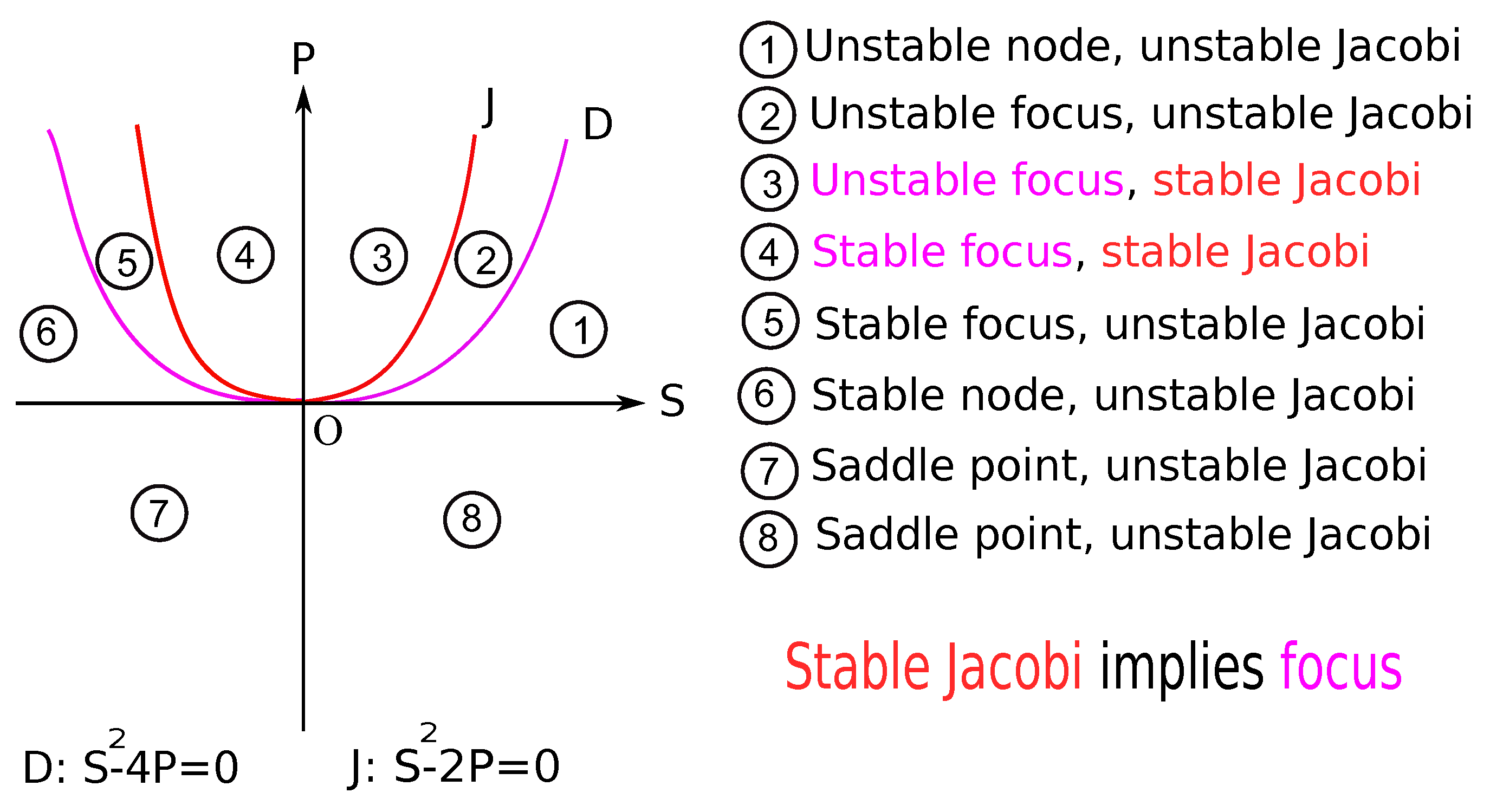
In order to more clearly represent the relationship between linear (or Lyapunov) stability and Jacobi stability for two-dimensional systems, we will consider the following diagram with respect to $S={\lambda }_1+{\lambda }_2=trA$ and $P={\lambda }_1{\lambda }_2=detA$ (see Figure 1):

Figure 1. Relationschip between Lyapunov stability and Jacobi stability for 2D systems.

In particular, for the Rosenzweig–MacArthur predator–prey system (4), we have

$$S^2-4P=\frac{b^2\delta B}{{(c-\delta )}^4}and{S}^2-2P=\frac{b^2(A^2+\delta B)}{2{(c-\delta )}^4}.$$

Then, we obtain the following result:

Theorem 11.

If the equilibrium point $E_2$ exists, then it is Jacobi-stable if and only if $B<0$ and $A^2<-\delta B$, where $A=-\delta \left[\right(b\delta +\delta -c)+bc]$ and $B=\delta {(b\delta +\delta -c+bc)}^2+4c(b\delta +\delta -c){(c-\delta )}^2$.

Because $A^2+\delta B=2\delta E$, the parameter $\delta >0$, which represents the death rate of the predator, plays an unexpectedly crucial role in the Jacobi stability of this system.

6. Examples and Discussion

Let the Rosenzweig–MacArthur predator–prey system (4) be expressed as follows:

$$\left\{\begin{array}{ccc}\hfill \dot{x}& =& x\left(-x^2+(1-b)x-y+b\right)\hfill \\ \hfill \dot{y}& =& y\left((c-\delta )x-\delta b\right)\hfill \end{array}\right.,$$

where b, c, $\delta >0$ and $x_1,x_2\ge 0$.

In order to illustrate the local dynamics of the predator–prey system, we will provide some concrete values for the three parameters of the system: b, c, and $\delta$. These particular systems will give us the confirmation of the previously obtained theoretical results, and they will also reveal to us that we cannot infirm or confirm Conjecture 2 from [12] by this approach.

From the point of view of Jacobi stability, only the equilibrium point $E_2$ can satisfy this property. More precisely, $E_2$ is Jacobi-stable if and only if $0<b\delta <c-\delta$ and $E<0$, where $E=B-2c(b\delta +\delta -c){(c-\delta )}^2$.

Example 1.

If $b=1.5$, $c=3.5$, $\delta =1$, then we have the equilibrium point $E_2$ with the coordinates $x=0.6$, $y=0.84$ and $A=-4.25$, $B=-69.438$, $E=-25.688$. Then, $E_2$ is Jacobi-stable with $A<0$ and $b\delta +b+\delta -1-c=-0.5<0$, such as in Conjecture 2 from [12].

Example 2.

For $b=0.2$, $c=0.8$, $\delta =0.5$, we have $E_2\left(0.33,0.35\right)$, with $A=0.02$, $B=-0.0568$, $E=-0.028$. Then, $E_2$ is Jacobi-stable with $A>0$ and $b\delta +b+\delta -1-c=-1.0<0$.

Example 3.

For $b=1.2$, $c=2.5$, $\delta =1$, we have $E_2\left(0.8,0.4\right)$, with $A=-2.7$, $B=0.54$, $E=3.915$. Then, $E_2$ is Jacobi-unstable with $A<0$, $B>0$, $E>0$, and $b\delta +b+\delta -1-c=-0.1<0$.

Example 4.

For $b=0.1$, $c=0.6$, $\delta =0.5$, we have $E_2\left(0.5,0.3\right)$, with $A=-0.005$, $B=-0.00115$, $E=-0.00055$. Then, $E_2$ is Jacobi-stable with $A<0$ and $b\delta +b+\delta -1-c=-0.95<0$, such as in Conjecture 2 from [12].

Example 5.

For $b=1.5$, $c=2.9$, $\delta =1$, we have $E_2\left(0.78947,0.48199\right)$, with $A=-3.95$, $B=-1.1479$, and $E=7.2273$. Then, $E_2$ is Jacobi-unstable with $B<0$, $A<0$, but $b\delta +b+\delta -1-c=0.1>0$, as in Proposition 1 from [12].

Example 6.

For $b=1.5$, $c=3.1$, $\delta =1$, we have $E_2\left(0.71429,0.63265\right)$, with $A=-4.05$, $B=-16.408$, and $E=-0.0027$. Then, $E_2$ is Jacobi-stable with $B<0$, $A<0$, but $b\delta +b+\delta -1-c=-0.1<0$, such as in Conjecture 2 from [12].

Example 7.

For $b=1.5$, $c=3$, $\delta =1$, we have $E_2\left(0.75,0.5625\right)$, with $A=-4$, $B=-8$, and $E=4$. Then, $E_2$ is Jacobi-unstable with $B<0$, $A<0$, and $b\delta +b+\delta -1-c=0$.

Example 8.

For $b=0.1$, $c=0.58$, $\delta =0.5$, we have $E_2$ with the coordinates $x=0.625$, $y=0.2718$ and $A=-0.014$, $B=-5.344\times {10}^{-5}$, $E=1.6928\times {10}^{-4}$. Then, $E_2$ is Jacobi-unstable with $B<0$, $A<0$, and $b\delta +b+\delta -1-c=-0.95<0$.

Example 9.

For $b=0.5$, $c=2.5$, $\delta =0.5$, we have $E_2\left(0.125,0.5468\right)$, and $A=0.25$, $B=-69.875$, $E=-34.875$. Then, $E_2$ is Jacobi-stable with $A>0$ and $b\delta +b+\delta -1-c=-2.25<0$.

Example 10.

If $b=1.5$, $c=2.5$, $\delta =1$, then $x=1$, $y=0$, and $E_2=E_1$. We only have the $E_0$ saddle point and the $E_1$ saddle node.

Example 11.

If $b=2$, $c=1.5$, $\delta =1$, then $x=4$, $y=-18$, and $E_2$ is a virtual equilibrium. We have the $E_0$ saddle point and the $E_1$ stable node.

Therefore, if the equilibrium point $E_2$ exists, then it may or may not be Jacobi-stable, whether the hypothesis of Conjecture 2 from [12] is fulfilled or not.

7. Conclusions

In this work, we conducted a study on the Jacobi stability of the Rosenzweig–MacArthur predator–prey system using the geometric tools of the KCC theory. We reformulated the first-order nonlinear differential system into a system of second-order differential equations (SODE) in order to determine the five geometrical invariants of the KCC theory. We calculated the first and the second invariant of the Kosambi–Cartan–Chern theory, and we were able to confirm that the third, fourth, and fifth invariants are all with null components, and that the Berwald connection vanishes. Furthermore, we determined the nonlinear connection associated with the semispray (SODE), and we computed the deviation curvature tensor at each equilibrium point in order to determine the Jacobi stability conditions.

Moreover, in order to compare these two approaches, a comparative analysis of the Jacobi stability and the Lyapunov (linear) stability near equilibrium points was made. Additionally, the deviation equations near every equilibrium point were determined. A next approach could be the performance of a computational study on the time variation of the deviation vector and its curvature in order to demonstrate the behavior of the Rosenzweig–MacArthur predator–prey system near the equilibrium points.