1. Introduction
Close approach (or Swing-By) are maneuvers where the spacecraft approaches a celestial body and uses the gravity of this body to modify its trajectory. The change is made in the velocity vector of the spacecraft, so the energy and angular momentum of the spacecraft with respect to the main primary of the system are modified, generating an asymmetric trajectory that can be used to achieve the goals of the mission. With respect to the secondary body of the system, the approached body, the trajectory follows the principle of conservation of energy, which generates a trajectory that is symmetric with respect to the periapsis line of the hyperbolic incoming trajectory. The more popular application of this maneuver is to send a spacecraft to targets like planets, moons or asteroids or to make the capture or escape of the spacecraft relative to the celestial body. This is a type of maneuver that is well known in the literature, and it has already been used in several space missions, usually with the objective of fuel economy [
1,
2,
3,
4]. A basic study of this maneuver is presented in [
5].
In addition to the pure version of the Swing-By maneuver, which uses only the gravity field of the body approached and the geometry of this passage to give or remove energy of the spacecraft, there are some options of maneuvers that combine different forms of propulsion to increase the flexibility of the maneuver, both in terms of optimizing the consumption and/or following constraints of the mission [
6,
7,
8,
9,
10,
11,
12,
13,
14,
15,
16,
17,
18]. The reason to consider those variants of the maneuver is to have more flexibility to achieve the goals of the missions, like gaining or loosing extra energy, or to pass by given regions of space, which would not be possible using only the gravity part of the maneuver.
Considering the use of an engine, propulsion combined with close approaches can give good results in terms of controlling the trajectory of the spacecraft during the close approach but still giving extra energy to the spacecraft. The point of having more control of the trajectory is particularly important when the mission occurs in strongly perturbed environments, similar to missions to the moons of the solar system or asteroids [
19,
20,
21,
22,
23]. In that sense, powered impulsive gravity assisted maneuvers have been considered in the literature for some time now [
7,
8,
9,
10,
11,
12,
13].
The use of a low continuous thrust [
24,
25,
26] has the advantage of having a high specific impulse, thus consuming less fuel. Another advantage of low continuous thrust is the possibility of having more control over the trajectory of the spacecraft, so allowing more flexibility in the maneuvers. In 1998, the Deep Space 1 mission, carried out by NASA, and the Smart 1 mission developed by ESA in 2003, showed the effectiveness of a continuous-thrust propulsion system [
27,
28]. Those missions opened the path for the study and exploration of the combination of close approach maneuvers and low thrust propulsion. Casalino et al. [
7] sought strategies to maximize the spacecraft energy, payload and engine operating time, with the goal of making a spacecraft to escape the solar system using a flyby around Jupiter and Venus. Later, McConaghy et al. [
29] created a trajectory design and the optimization of trajectories in two steps: first looking for potential trajectories and then optimizing the most promising ones. The study focused on missions to Vesta, Tempel 1, Ceres, Jupiter and Pluto. Pascale et al. [
30] proposed an automatic method for a preliminary definition of the complex interplanetary transfer, characterized by multiple Swing-Bys combined with continuous or impulsive maneuvers. The objective was to achieve a new methodology for the description of continuous thrust arcs based on an inverse method with a global optimization algorithm. In 2006, [
31] studied the combination of continuous thrust and gravity assisted trajectories for missions to Jupiter via swing-by in Venus, Earth and Mars, considering the years from 2010 to 2045. They used sinusoidal exponential and conical arcs as initial guesses to obtain the trajectories. They also found that the performance of trajectories involving intermediate flybys is highly dependent on the year of the mission. In [
32], a transfer from Earth to Europa using electric propulsion and multiple gravity assisted maneuvers was considered. Different forms of optimization for the Swing-By were used. In 2010, [
33] combined a Swing-By and continuous thrust to reach several asteroids.
More recently, [
13] developed a method to avoid the difficulties of solving the optimization problem of the interplanetary trajectory of the spacecraft with continuous-thrust using a sequence of Swing-Bys. Reference [
34] studied the interplanetary trajectories for a spacecraft leaving Earth using continuous thrust and making flybys with Mars on its path to Jupiter. In [
35], a method for designing an Earth–Mars trajectory for a spacecraft equipped with electric propulsion is proposed, which also uses gravity-assisted maneuvers. Reference [
36] developed a multi-gravity assist maneuver combined with low thrust, using an optimization software known as LInX (Low-thrust Interplanetary eXplorer).
Looking in more detail at the literature, we see that reference [
11] analyzes the effects of different geometries and characteristics of a single impulse applied during the Swing-By maneuver in the energy variations of the spacecraft. In particular, it finds the locations of the extreme variations with the objective of changing the trajectory of the spacecraft to send it close enough to the body to be captured or to collide with it. To extend this idea, the present paper aims to analyze and understand the effects of the application of continuous thrust propulsion during one arc of the trajectory close to the Swing-By, a different type of maneuver. The idea is to verify the variations of energy that the combination of Swing-By and continuous thrust can make and compare the results with the variations given by a pure gravity assisted maneuver followed by a continuous thrust applied in a region far from the celestial body. A combined maneuver such as this one may be used to increase the control of the trajectory of the spacecraft in the crucial moments of the closest approach, but it is interesting to know the effects of this combination in the variations of energy given to the spacecraft. In this way, a continuous thrust propulsion arc can be applied to the spacecraft to adjust its orbit and the Swing-By, so that the spacecraft, in addition to observing the celestial body from certain given points, can obtain extra variations of energy to follow its path to reach other goals. In that line, it is important to study the effects of this combined maneuver in the variations of energy of the spacecraft, such as the extension, location and magnitude of the arcs. For a short arc, a thrust with very low magnitude may not have effects that are large enough to be measured but larger magnitudes for the propulsion can make differences in the maneuver, in particular by changing the geometry of the close approach. The study of the level and duration of the thrust required to make important effects and how to use this thrust for the benefit of the mission are the main goals of the present research. Of course, for a real mission, it is important to also consider several other aspects, such as the level and origin of the propulsion (electrical, nuclear, solar, etc.), the options for the control (direction of the impulse, fixed or variable level of thrust, etc.), the length of the propulsion arcs, the geometry of the maneuver and more.
The proposed numerical method can be validated by approximating the continuous propulsion by a single impulse, such that the solutions obtained here can be compared to those presented in the powered Swing-By literature previously cited.
2. Close Approach Maneuver
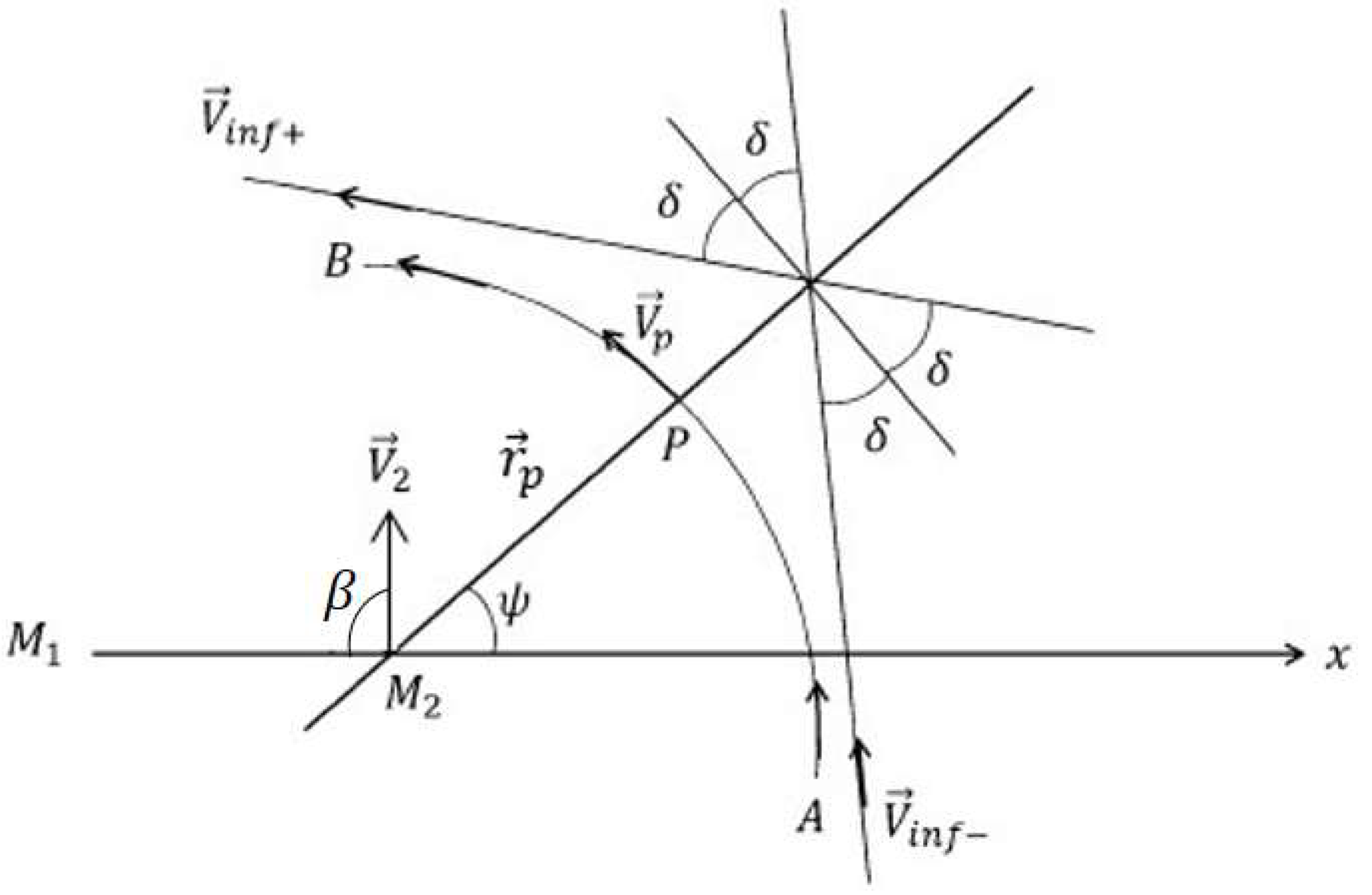
A maneuver can be considered to be a “pure gravity close approach” (or “pure gravity Swing-By”) when the only forces acting in the trajectory of the spacecraft are the gravity fields of the two massive bodies involved in the dynamics. If high accuracy is not required, it is possible to model this dynamics using the “patched-conics” approximation, which considers that the close approach is instantaneous [
5], so the position vector is assumed to be constant during the Swing-By. For an ideal hyperbolic orbit, not subjected to perturbations or propulsion, the modulus of the incoming relative velocity
must be equal to the modulus of the outgoing relative velocity
, both with respect to the closer body. Therefore, the outgoing relative velocity vector is just rotated by the gravity field of the celestial body by an angle
[
5], with respect to the incoming velocity vector, as shown in
Figure 1. Then, we can see that:
With
and
[
5], where
is the periapsis distance, which is the minimum distance that the spacecraft passes by the center of the body considered for the maneuver, and
is the mass parameter of this body. If propulsion is involved, the Swing-By does not depend only on gravity forces, but it is also dependent on the propulsive part of the mission. The total curvature of the maneuver is no longer
and
can be different from
.
This problem can be solved numerically, and we can replace the “patched-conics” approximation by the restricted three-body problem as the dynamical model, where is the main body of the system with the largest mass; is the secondary body with mass ; and the spacecraft () is assumed to have a mass , so it is disregarded. This model gives more accurate results:
The maneuver is shown in
Figure 1, in the rotating frame.
is the periapsis point,
is the magnitude of the velocity of the spacecraft at
,
the angle of approach (angle between the
-axis and
) and
the velocity vector of
relative to the center of mass of the system. If the maneuver occurs around a system with elliptical orbits,
. The distance
is
, where
is the eccentricity,
the true anomaly and
the semi-major axis of the orbit of
around
.
Relative to the inertial frame, the incoming velocity (
) and the outgoing velocity (
) of the spacecraft at the limits of the sphere of influence of
, both relative to the main body of the system, can give us the variations in velocity (
), energy (
) and angular momentum (
), as given by Equation (2).
besides that, we have:
If the system under study is elliptical, , where is the angle between and the -axis, which is given by , with the radial velocity of .
Some important observations can be made based on studies of the pure Swing-By maneuver. They are:
- -
The spacecraft loses energy due to the gravity when the closest approach occurs in front of
, i.e.,
, with a maximum loss for
[
5].
- -
The spacecraft gains energy due to gravity, when the closest approach occurs behind
, i.e.,
, with a maximum gain for
[
5].
- -
For
or
, the gravity does not change the energy of the spacecraft, so the variation is zero [
5].
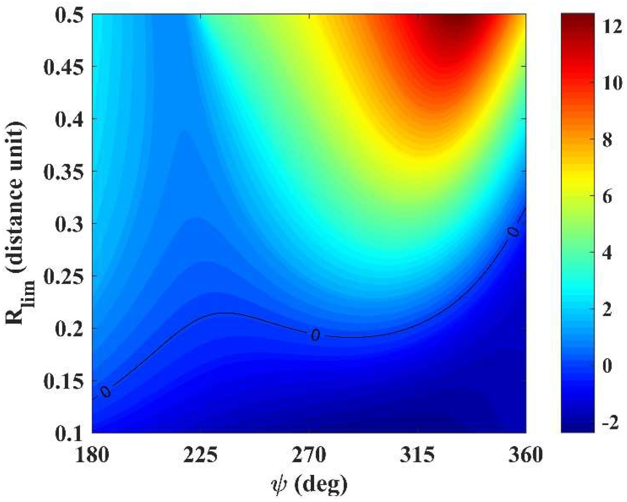
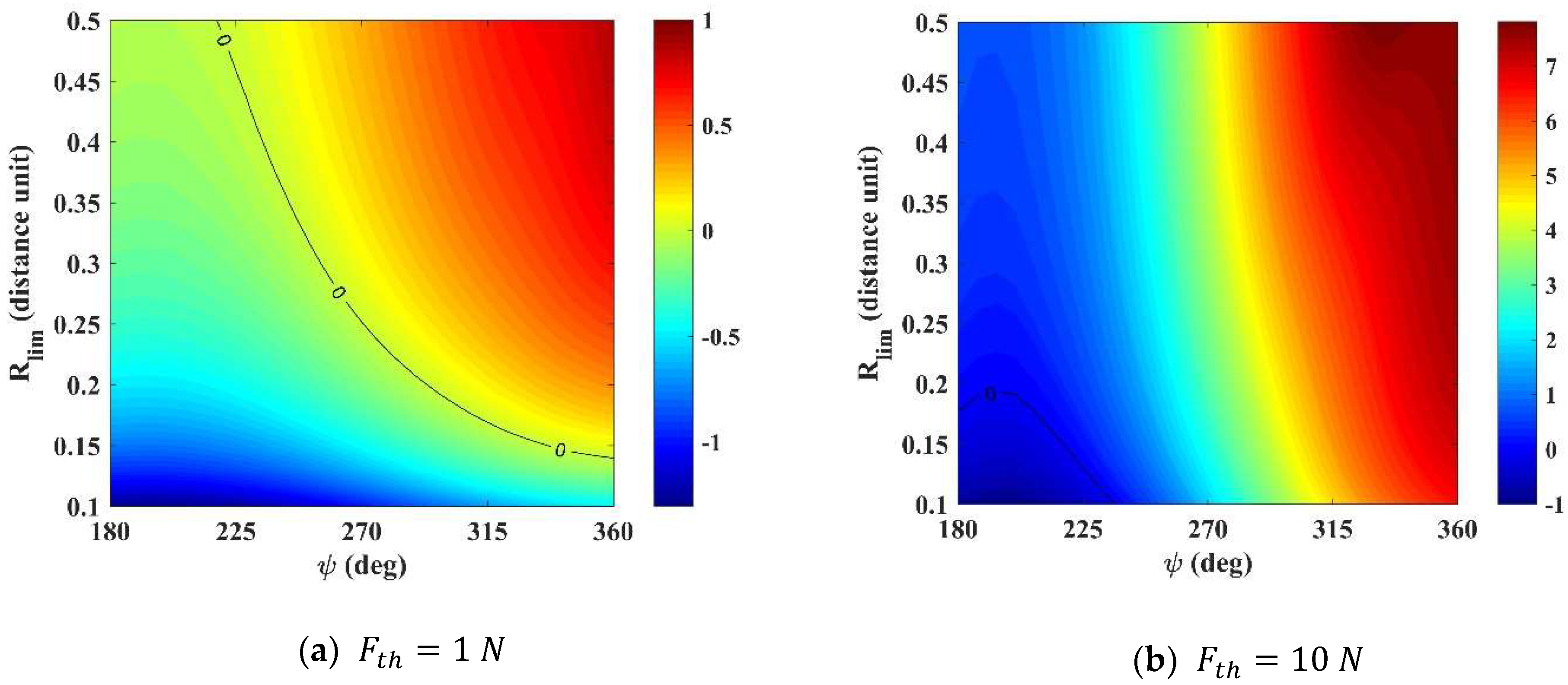
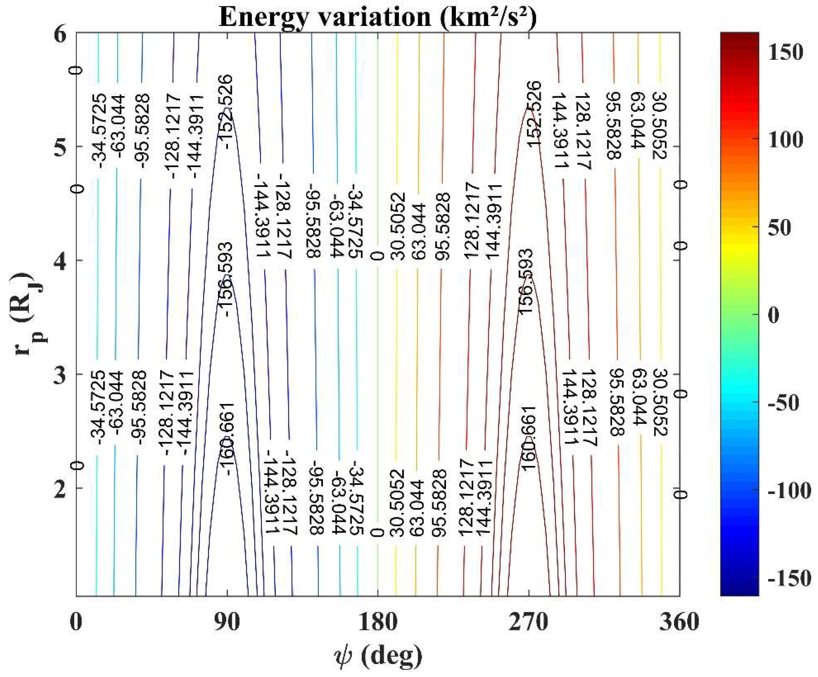
Figure 2 shows the energy variations for a system with circular orbits,
(similar to the Sun–Jupiter system),
,
, different values for
(in
–radii of Jupiter) and
.
3. Statement of the Problem
It is assumed that the maneuver is made using a continuous thrust combined with a close approach maneuver, using a Keplerian model for the gravitational part of the dynamics. In this situation, we have a hyperbolic orbit for the spacecraft relative to
during the maneuver, disturbed only by the thrust. For this problem, the characteristics of the engine are defined by the predetermined values of power (
), specific impulse (
), thrust efficiency (
) and gravity on the surface of the Earth (
), i.e.,
[
37].
Then, we define the “Swing-by combined with continuous low thrust” maneuver as SBCT maneuver; the “pure gravity Swing-By” as SB maneuver and the “pure propulsive maneuver” (or continuous thrust maneuver) as CT maneuver.
Let us consider the state vector
, written in the rotating frame, and its time derivatives
, being
and
(the position, velocity and acceleration components of
) and
and
(the position, velocity and acceleration components of the spacecraft
).The equations of motion, in the rotating frame, are
and
, where
is the angular velocity of the system, in dimensionless units,
and
are the partial derivatives of the potential
acting in the spacecraft with respect to
and
(Equation (4)), and
is the thrust acceleration vector (Equation (5)).
where
represents the position of
in the rotating frame.
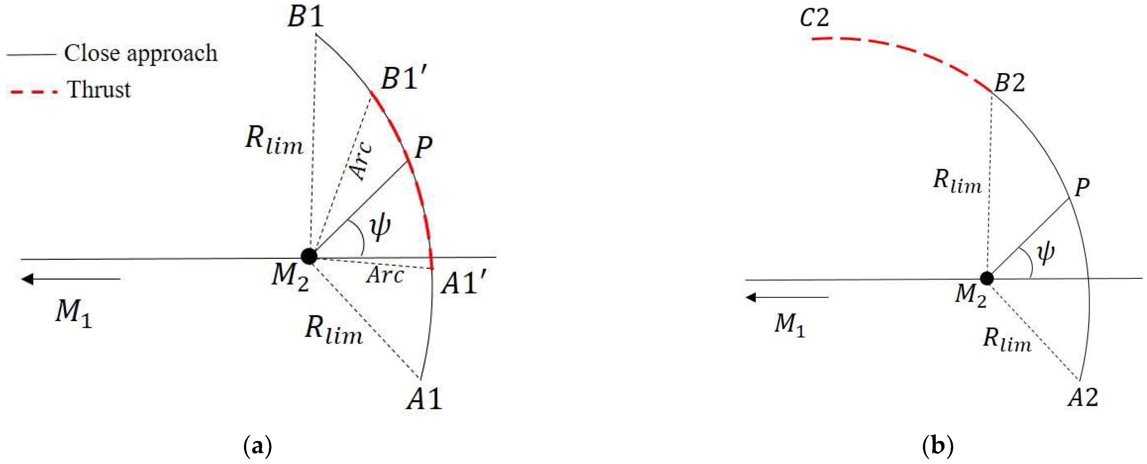
The SBCT maneuver can be divided into five parts (
Figure 3a). The first part considers that the spacecraft is travelling in the
system but is far from
. In this part of the trajectory, we consider that the orbit of the spacecraft is Keplerian and we measure its two-body energy,
, velocity and angular momentum, with respect to
. In the second part, the spacecraft moves closer to
and, from this point (
in
Figure 3a), its motion is governed by the equations given by the Restricted Three-Body Problem. The spacecraft then follows its trajectory and, at point
, the thruster is activated, starting the third part of the maneuver. During this phase, the gravity fields of
and
and the thrust are the forces governing the motion of the spacecraft. It is assumed that the thrust acceleration vector (
) has the direction and sense defined by the angle
, measured by its displacement from the velocity vector of the spacecraft.
if
, the thrust acceleration vector has the same direction and sense of the velocity vector of the spacecraft; if
, the thrust acceleration vector points to a direction that makes a clockwise angle from the velocity vector of the spacecraft; if
, the thrust acceleration vector points to a direction that makes a counterclockwise angle from the velocity vector of the spacecraft. The angle
follows the definition:
This phase of the mission finishes when the spacecraft reaches the predetermined distance or time to turn off the engine () and the thruster is disabled. Then, the fourth phase of the maneuver begins. The spacecraft goes from to , with its motion governed by the Restricted Three-Body Problem again. Finally, the last phase of the maneuver starts at a point equivalent to . The spacecraft is far from , and its motion can be again considered to be Keplerian around . This last phase completes the maneuver and the final Keplerian orbit around can be identified, so energy, velocity and angular momentum after the maneuver can be obtained.
Points
and
define the period/distance that the engine is working (
Figure 3a). The
is measured from the center of
in radii of the secondary body. The duration of the SB maneuver, on the other hand, lasted as long as necessary to follow the predefined distance (
) for points
and
. Therefore,
is the distance from the center of
to the point
and from the center of
to the point
.
Computationally, the algorithm is developed using numerical integrations in positive and negative senses of time, from the periapsis of the orbit, predetermined by the initial conditions
,
and
(point
,
Figure 3). The sequence of the maneuver is as follows:
- -
The sequence starts at the periapsis of the orbit of the spacecraft (initial state vector).
- -
The equations of motion of the spacecraft are integrated for negative times, adding the propulsive force to the gravitational attraction.
- -
The integration of the equations of motion, including the thruster, is interrupted when the spacecraft reaches point .
- -
The integration follows only with the gravitational effect, and it is interrupted when the spacecraft reaches point .
- -
After that, the orbit of the spacecraft is obtained (velocity and energy).
- -
In the sequence, again beginning from the periapsis, the equations of motion are integrated forward in time, also with the thruster active.
- -
The numerical integration with the thruster is interrupted when the spacecraft reaches point .
- -
After that, the numerical integration follows only with the gravitational forces until the spacecraft reaches point .
- -
Then, the orbit of the spacecraft is obtained again (velocity and energy).
The engine is assumed to have constant mass, due to its low mass consumption.
Consider
the initial state vector, where
is the velocity of
,
is the magnitude of the velocity of the spacecraft at the periapsis and
the angle of approach (angle between
-axis and periapsis position vector).
Figure 3b shows the combined maneuver (SB plus CT) used to compare and analyze the relative efficiency in energy gains of the SBCT. The algorithm is developed based in numerical integrations made in positive and negative senses of time, starting from the periapsis (point
in
Figure 3). When starting the maneuver from the same point
, the spacecraft does not reach the same periapsis conditions (point
) for the close approach in both maneuvers. Therefore, the integration has to be carried out reversely in time, starting from point
. The consequence of the different starting points is something to be analyzed separately, but it does not belong to the scope of this work, which is focused on the close approach itself. To analyze the SB plus the CT maneuver performance we followed the steps:
- -
The pure Swing-By () starts at and ends at (defined by );
- -
From , the thruster is turned on and the spacecraft goes to , where the thruster is turned off;
- -
In the trajectory between and , the motion of the spacecraft is governed by the gravitational force of and the thrust force;
- -
The duration of the propulsive part of the maneuver during the
arc is the same as in the arc
shown in
Figure 3a;
- -
is calculated by subtracting the energy when the spacecraft in at the point from the energy of the spacecraft when it is at .
The dashed red curve represents the propelled part of the maneuver, while the continuous black line shows the part of the maneuver that has only gravity forces involved. From these maneuvers, it is possible to verify the conditions to obtain an optimal effect from the close approach and continuous thrust occurring simultaneously, so we can compare the results obtained with the ones given by the maneuver that uses a pure gravity close approach.
If and , the thruster is active for a period equals to the time used to calculate the SB maneuver, that is, a large propulsion arc is used and it acts during the same time that the gravity of is working. Situations under these conditions will be analyzed in the present research.
The size of the system directly influences the magnitude of the parameters of the maneuver, because the Swing-By works better when performed around bodies with larger mass and, consequently, stronger gravity fields. Let us now consider a system that is similar to the Sun–Jupiter system. We also assume that the approach velocity () is equal to 6.3 km/s, that is, 10% above the minimum value given by a Hohmann transfer coming from Earth. The initial periapsis radius () of 1.05 radius of the secondary body is used. Therefore, from the conservation of energy, the periapsis velocity is , where is the mass parameter of Jupiter. The continuous thrust is varied from N to N. A weaker thrust is considered and when a higher continuous thrust is available. Remember that, if necessary, we can consider more than one engine in the mission, with all of them applying the thrust in the same direction, to increase the magnitude of the total thrust.
Let us define the distance unit as the distance , which is about 778,340,821.0 km in our situation. One unit for the velocity is the orbital velocity of , which is around 13.1 km/s in our simulations, and the unit of time is 689.1 days, selected so that the orbital period of the primaries is 2π.
4. Efficiency in Energy Gain of the SBCT Maneuver
We will measure the energy variation (
) for the different maneuvers presented in this paper, taking into consideration that the thrust force is applied in the direction of the motion of the spacecraft (
) and considering all the possibilities for the angle of approach. Despite the fact that the region of energy gains due to gravity is
[
5], a mission can reach the celestial body with an angle not favorable for the gain of energy.
The maps of energy variations are not shown here, because they have a behavior similar to those coming from a pure gravity maneuver (
Figure 2), with only small shifts in the regions caused by the thrust. The spacecraft has its energy reduced in the interval
, with larger reductions for the lowest thrust values. Propulsion with higher values minimizes these reductions. For the highest values of thrust and
around zero, there is a small region of positive variations. It happens because, according to [
5], in pure gravity, SB maneuvers the effect of the close approach in the variation of energy is zero for
or
and
, so the propulsion stands out in this region. There are energy gains in the region
, with the values increasing for higher thrust values.
To find out which conditions are more advantageous to the use of the SBCT maneuver with respect to energy gain, we analyzed the differences in the energy variations between both maneuvers (SBCT and the SB plus CT), for the same direction and magnitude of the thrust and time.
is the energy variation of the spacecraft due to the Swing-By maneuver combined with continuous thrust (SBCT maneuver) and is the energy variation of the spacecraft in the SB plus CT maneuver.
Based on the analysis of energy variations, if and , the combined maneuver results in larger energy gains. If and , the SBCT results in smaller energy losses. For , those maneuvers have the same effect and, if and , the maneuver that combines continuous propulsion with a close approach brings smaller gains for the maneuver and larger losses of energy for and . Therefore, we consider the SBCT maneuver to be efficient for energy gains when and , because the maneuver provided extra energy for the spacecraft.
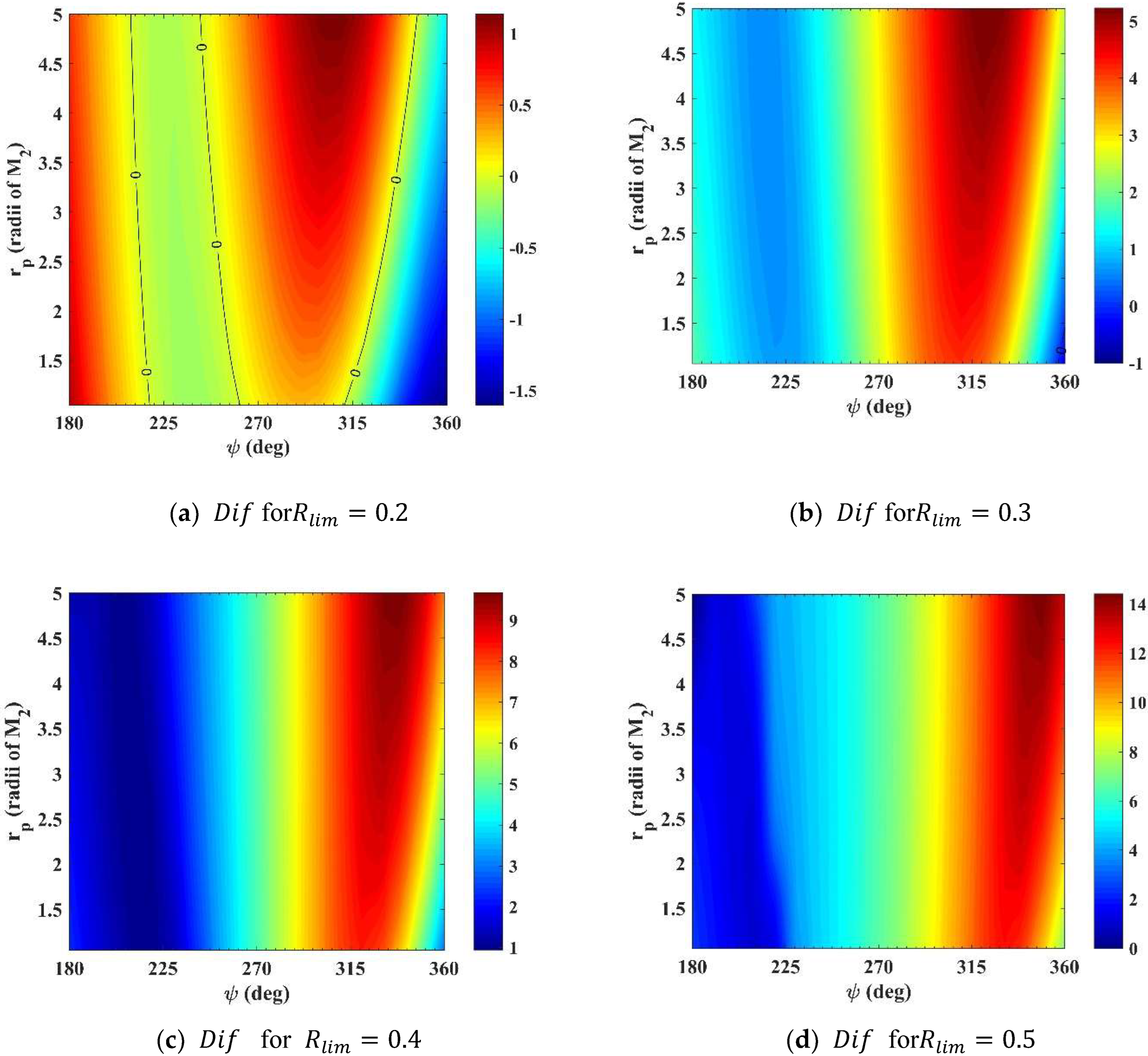
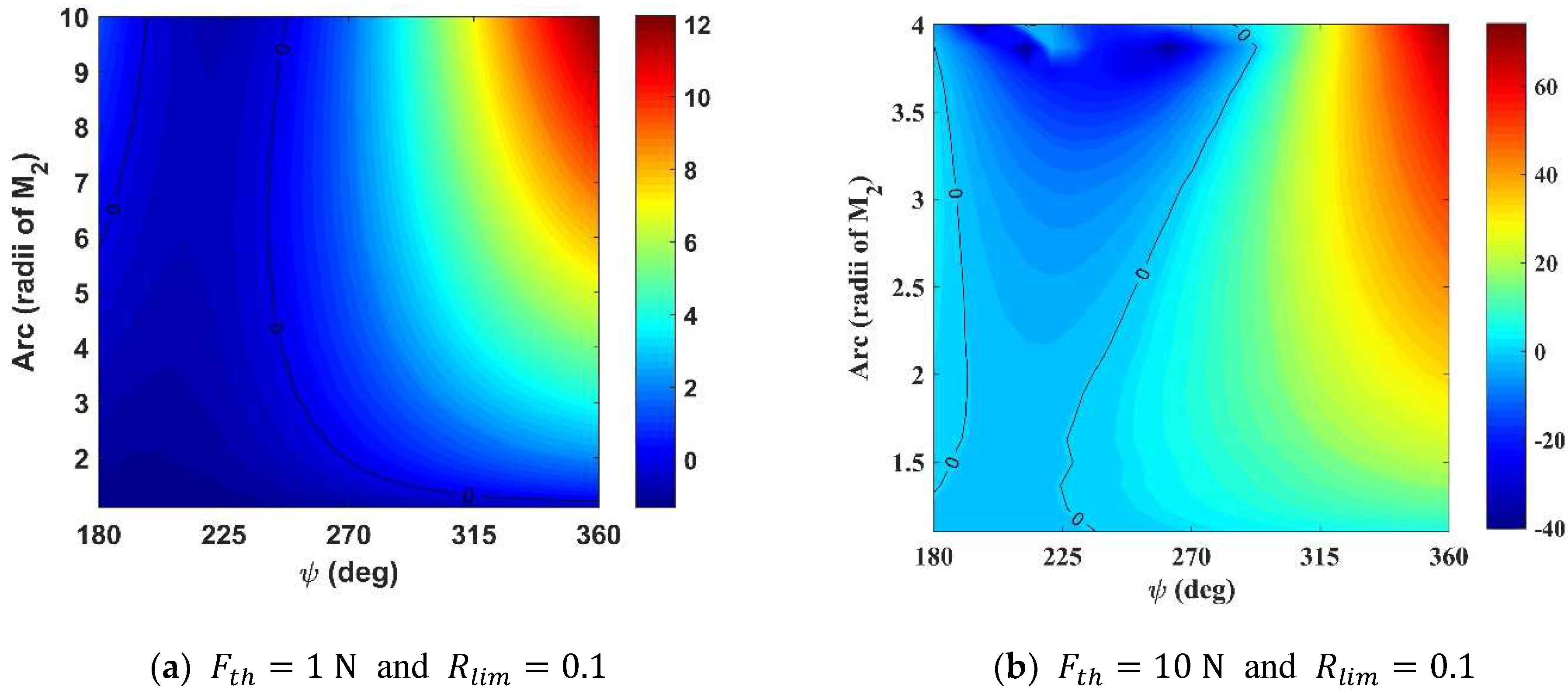
4.1. Conditions for Large Propulsion Arcs Using Lower Values for the Thrust
Let us consider that the propulsion arc has the same size of the SB maneuver, that is,
and
(
Figure 3a). Therefore, we have continuous thrust acting for a long time, whose limits are defined by
.
Figure 4 shows the differences in energy variations for different conditions.
The longer the integration time, the larger the energy gains due to the propulsive part of the maneuver. Smaller arcs, such as
(~251 days of active thruster), with small variations depending on the values of
and the thrust, see
Figure 4a, suffer a large effect from gravity and smaller effects from the thrust. When
the pure SB has its maximum loss of energy due to gravity, and the propulsion applied after the maneuver (SB plus CT) cannot compensate for this loss of energy. The thrust in the combined maneuver (SBCT), in the same region as
and works to minimize the losses of energy during the close approach, thus explaining the positive
in the region around
.
Observe that the SBCT maneuver is interesting for energy gains for
(~377 days of active thruster), and yet, in all these cases, there is a positive region of
for
, which suggests the minimum loss of energy. For slightly larger arcs of propulsion, as shown in
Figure 4b, the thrust and the SB are balanced, so the maximum differences are closer to the surroundings of
. In this situation,
due to gravity is null, with small gains after
and smaller losses before this point. The absolute maximum of
observed in the map belongs to the region of the losses of energy, but the local maximum for energy gain occurs for
and
km
2/s
2. Then, larger arcs (
, ~503 days of active thruster) make the thrust more significant, and it has a stronger effect when
is null for the pure gravity SB (
). For
(~1055 days of active thruster) and
(~1317 days of active thruster), there are positive regions around
and a region where
is zero for the pure gravity maneuver, but the thrust works to gain some variations of energy. In these cases,
results in sending the spacecraft to distant points, defeating the purpose of the maneuver, which is to observe the celestial body during the approach and then take advantage of the energy gain to modify the trajectory of the spacecraft, according to the goals of the mission.
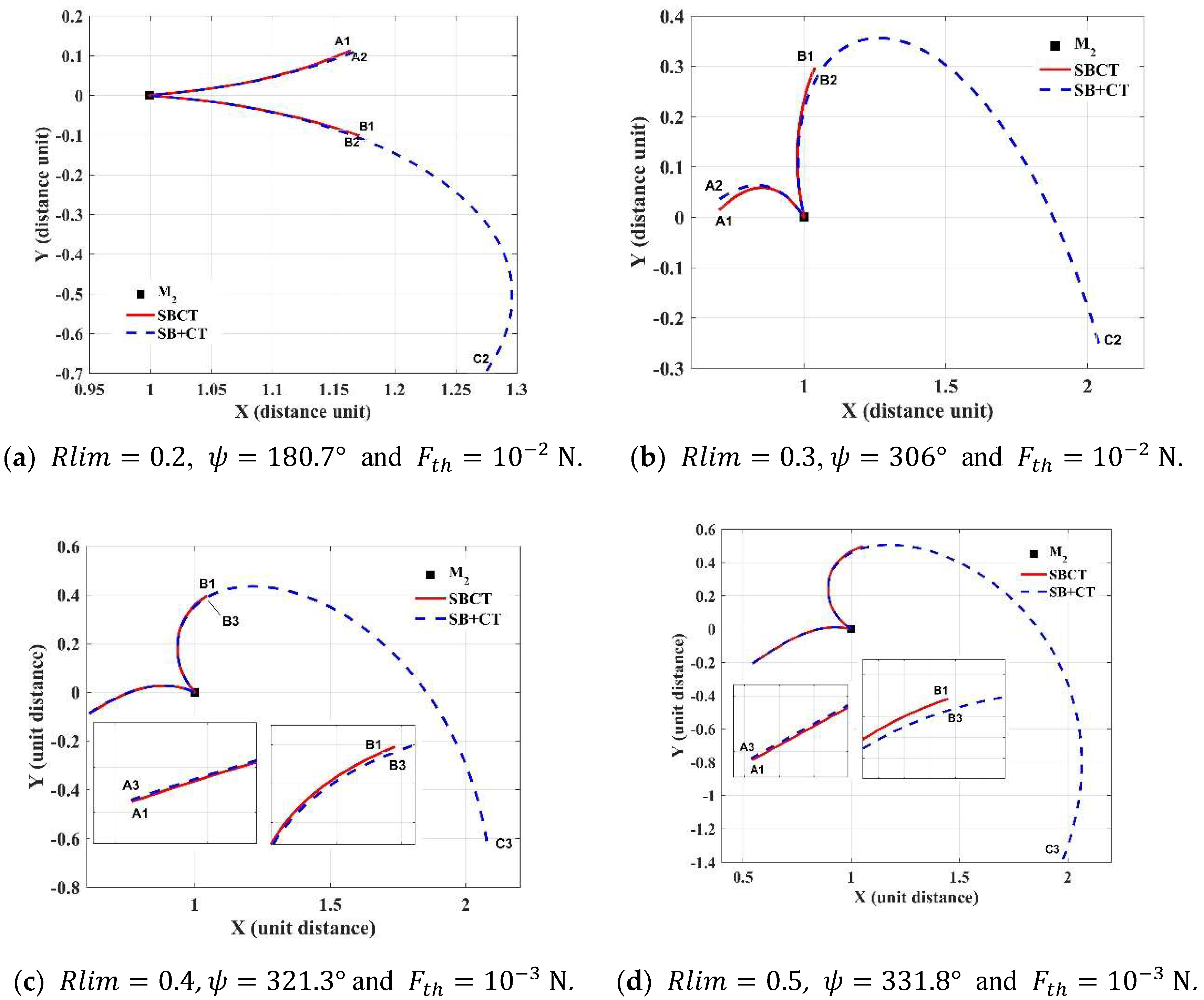
Table 1 shows the maximum difference between the energy variations (
).
The extreme conditions for
refer to the minimum energy losses for the spacecraft, since the equivalent
in SBCT and SB plus CT are negative. For
, the same situation occurs, but there is a local maximum on the map of the differences (
Figure 4b), whose condition refers to a situation of positive variations for the SBCT maneuver, approximately 201.7% of gain, given that
for the SB plus CT maneuver is negative. For
, equal to
and
, the conditions of the maximum
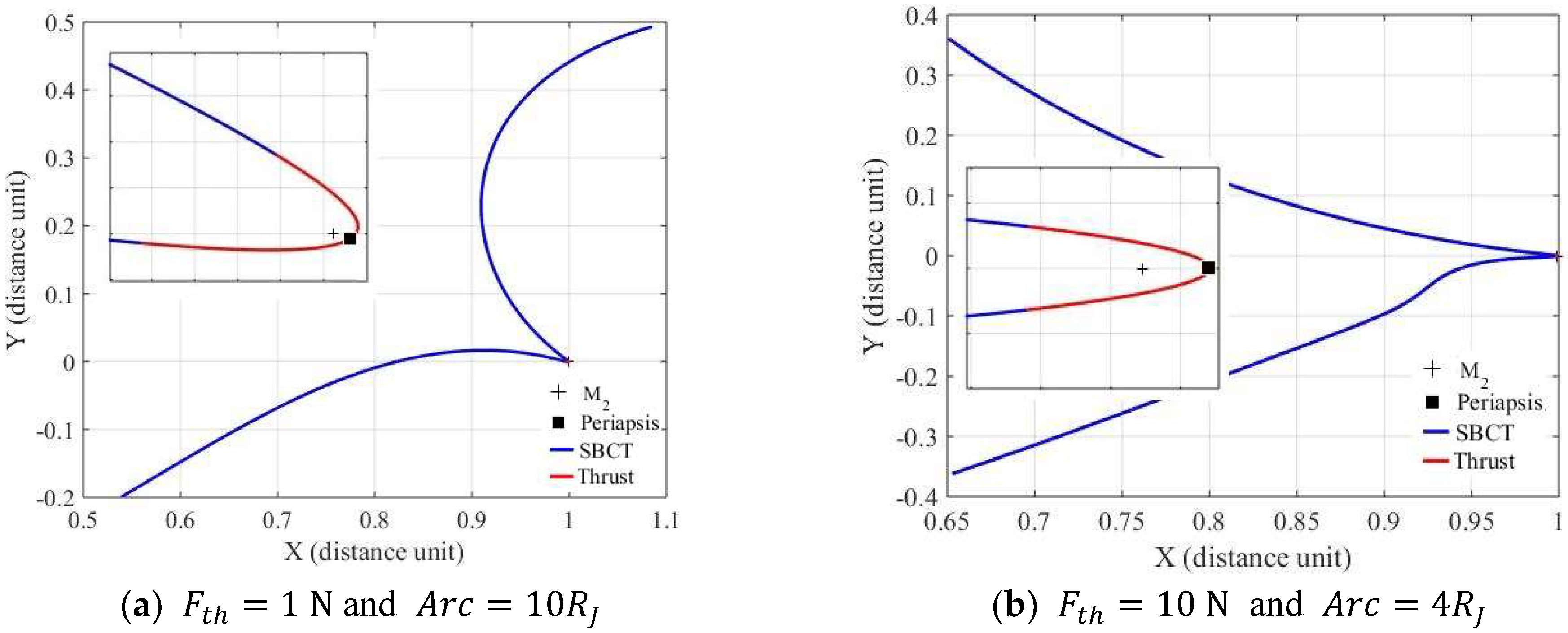
show the efficiency of the SBCT maneuver when the focus is on energy gains. They increase energy gains by 22.8%, 8.2% and 16.5%, respectively, compared to SB plus CT. The trajectories referring to the conditions shown in
Table 1 that result in more efficiency in energy gains for the SBCT maneuver are presented in
Figure 5.
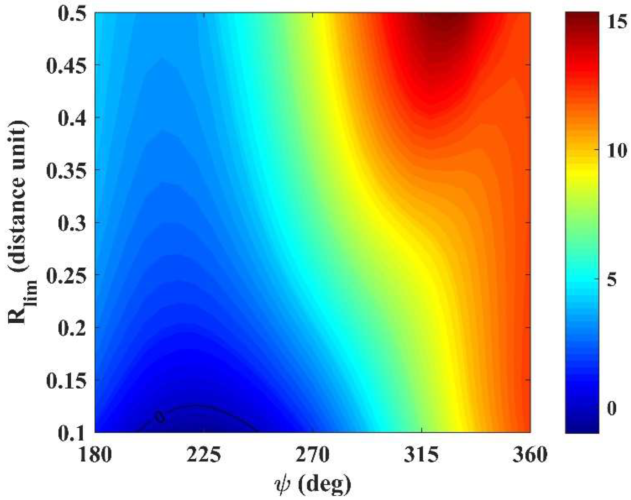
Figure 6 summarizes the efficiency of the SBCT maneuver for the conditions of energy gains, using different values of
and
. This figure gives us an overview of the efficiency of the maneuver. As expected, larger thrust arcs resulting from larger
increases the energy gains, with values of
above approximately 315°, where the energy variations are smaller due to the gravity aspect of the maneuver. The magnitude of the gain is larger for lower masses. This map also shows the region where using the SBCT is not the best option when
is approximately less than 0.2, given that the close approach followed by a thrust arc gives more energy to the spacecraft.
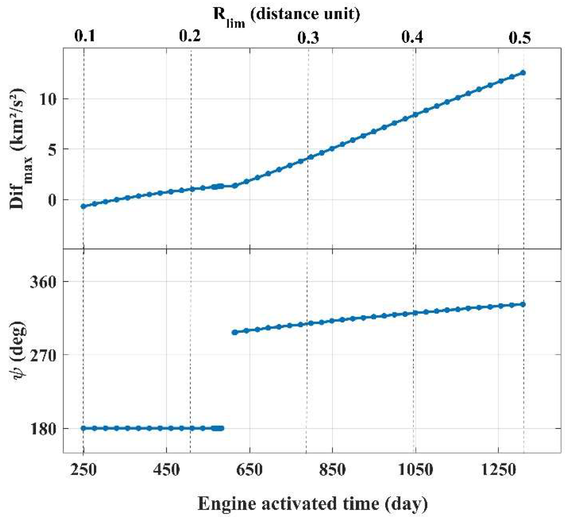
Figure 7 shows the maximum efficiency of
and their respective angle of approach, relative to
Figure 6, considering the time the engine is active (days). There is a pronounced increase in the maximum efficiency when the engine is activated for more than 600 days approximately, with angles of approach increasing from about
to
. The SBCT maneuver becomes efficient (
) with active engine times over
days.
In addition to the analysis of the variables related to the continuous thrust ( and engine activation time), we also analyzed the parameters related to the initial orbit of the spacecraft ( and ).
Figure 8 shows that the maximum efficiencies occur in higher values of
. This is correct, since the farther from the body the maneuver occurs, the smaller the effect of gravity, so the propulsive part of the maneuver helps to compensate for this loss, making the SBCT more efficient in these cases. For
, the maneuver is not efficient. For
the maneuver is efficient, and for
there is a negative region, where SB plus CT has better results.
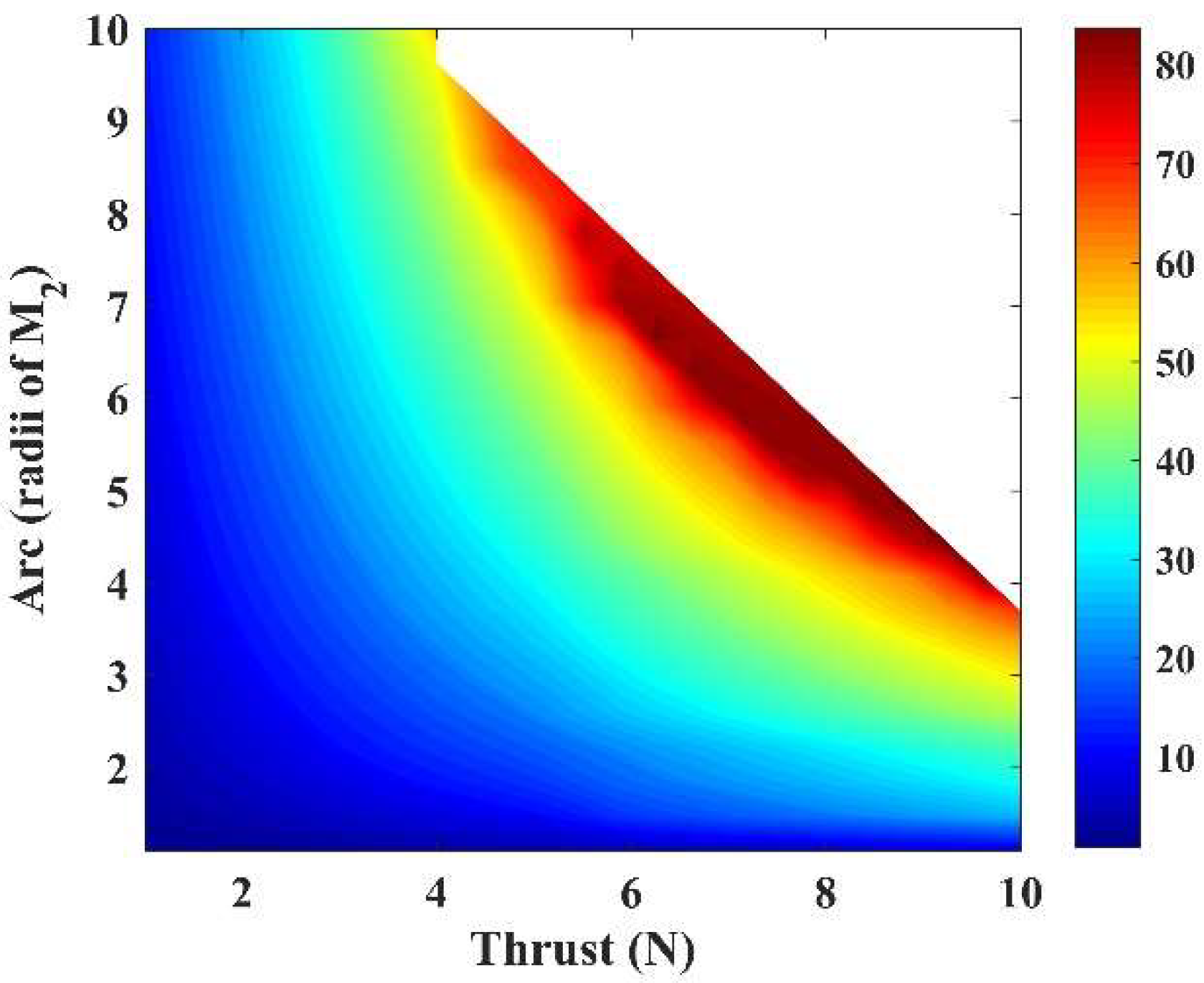
4.2. Conditions for Small Propulsion Arcs Using Higher Thrust
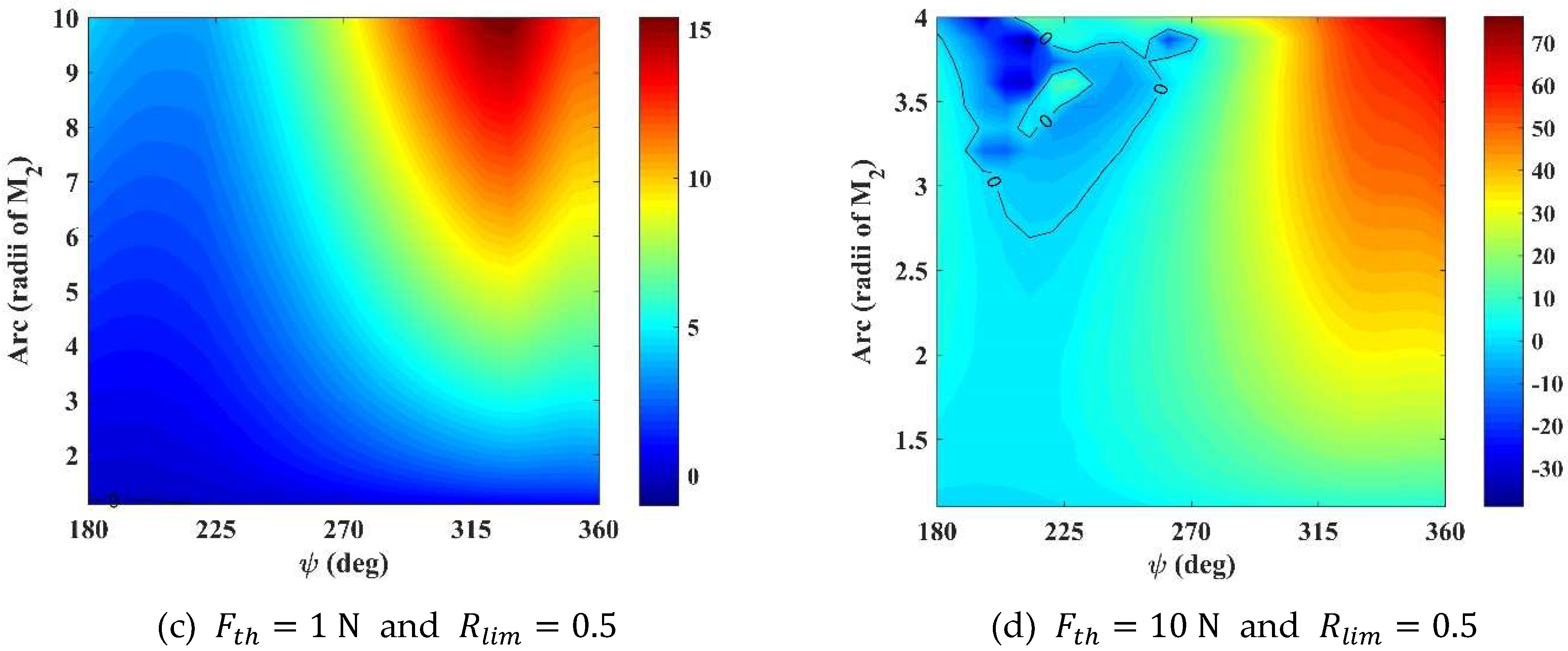
Let us analyze the efficiency of the SBCT maneuver when compared to the maneuver that uses SB and CT, for , using higher thrust () and smaller propulsion arcs (from 1.1 to 10 -radii of Jupiter). Consider that the positive magnitudes of the maps represent an efficient maneuver relative to the energy gain, i.e., there is extra energy coming from the SBCT maneuver compared to the situation where the maneuver is made in two steps.
Initially, we have the map of the thrust magnitude (
) versus “
”, which defines the length of the propulsion arc (
Figure 9). We fixed
and
.
Observe that the efficiency increases with the magnitude of these variables, reaching a maximum of about 89 km2/s2. The blank region represents situations of collisions or singularities due to the high magnitude of the thrust. These singularities will not be analyzed in the present work.
From this point, we will analyze the efficiency of the SBCT maneuver for each variable involved, always based on , which is a key parameter for the study of the efficiency.
Figure 10a,b shows the results for
, which means that the engine is active for approximately 0.298 h (1071.7 s). It is observed that there are differences in the magnitudes of the efficiency when comparing
with
. For
,
is 0.8849 km
2/s
2 (for
), while for
,
is 7.9217 km
2/s
2 (for
), i.e., approximately nine times higher. Note also that, for
, the value of
referring to the maximum difference is significantly far from
. This is explained by the larger magnitude of the force, which is now strong enough to compensate for the displacement of the region of zero variation of energy due to gravity and still remain more efficient. Even in this case, the region of non-efficiency (
) on the map (
Figure 10b) is significantly smaller than the equivalent region in
Figure 10a.
For
(
Figure 11), the integration time with active propulsion is approximately 15 h (~54,001 s). Despite the fact that the force is
, the longer time, compared to the results shown in
Figure 10a, gives a significant increase in the efficiency range. Note that the inefficient region is minimal, and it occurs for the smallest SB length (
) and in a small range of
. If we consider that
and
, there are collisions of the spacecraft with Jupiter for all conditions of
and
.
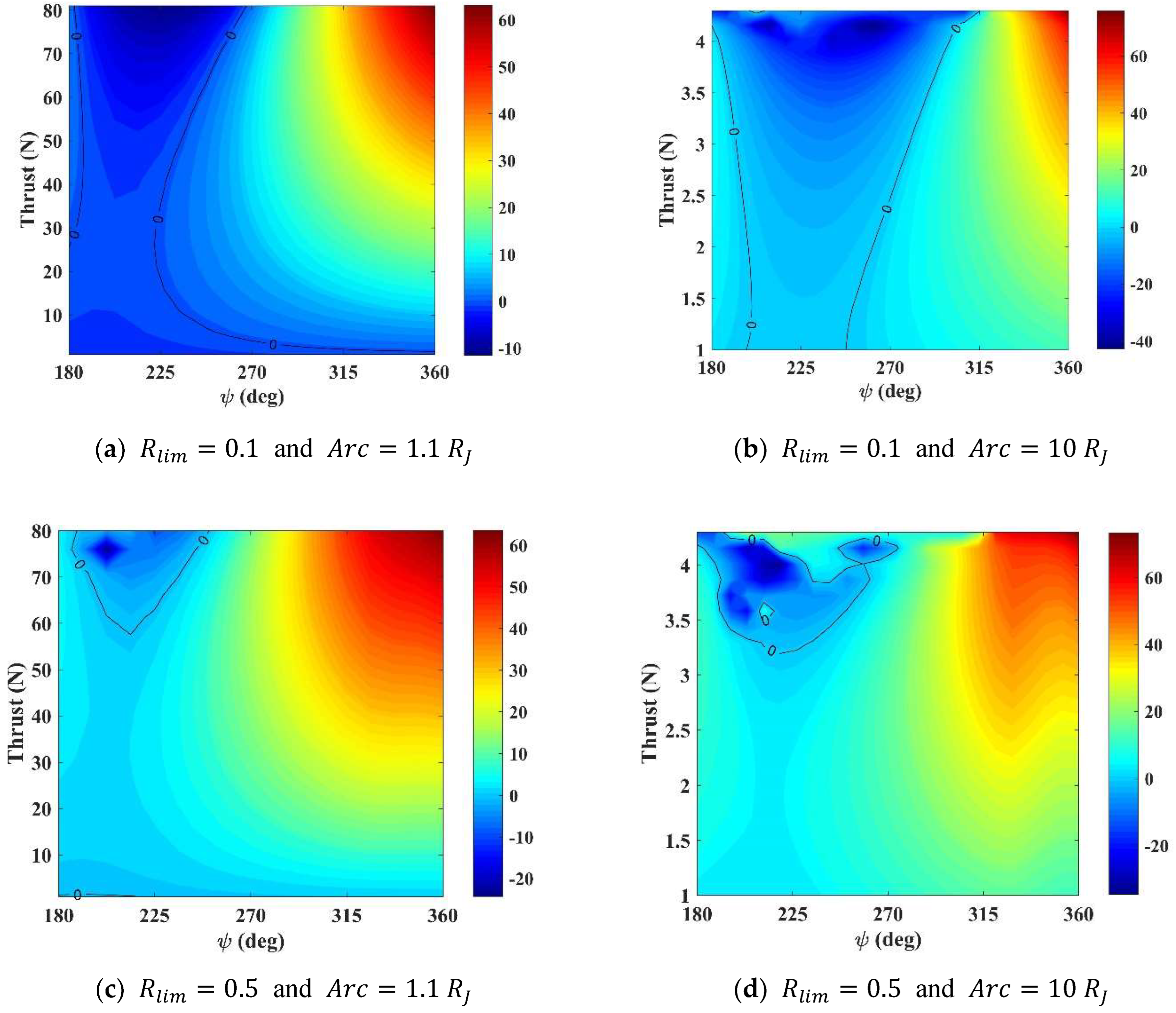
Now, looking at the results as a function of
, considering the highest and lowest values of the thrust and
, we have four plots that describe the behavior of the maneuver. For
,
and
(
Figure 12a,b), there are wide regions of non-efficiency for approximately
for all values of
. As expected, the magnitude of the range for
is much larger than the same magnitudes when using
, even in the case of non-efficiency, being
km
2/s
2 and
km
2/s
2, respectively. Larger propulsions have larger effects on the velocity of the spacecraft and, consequently, in the variations of energy.
For
Figure 12c,d we used
, therefore intensifying the effect of the gravity due to a longer SB and decreasing significantly the non-efficient regions. For
, the
km
2/s
2 and, for
,
km
2/s
2. Note that, for the situations where
,
is analyzed up to
, due to the frequent collisions, as shown in
Figure 9.
Figure 13 shows the efficiency of the SBCT maneuver for different magnitudes of the thrust considering values up to
, if we consider
to be independent from
. For
, the thrust increases to near 4
. Above this limit there are collisions and singularities.
From these previous data, the larger SB analyzed gave larger efficiency, because the spacecraft spends more time taking advantage of the effect of gravity. It is also known that a largest force acting on the spacecraft results in more energy gains from the SBCT maneuver; however, the force must be combined with the length of the propulsion arc so that it does not reach the regions of collisions or singularities (
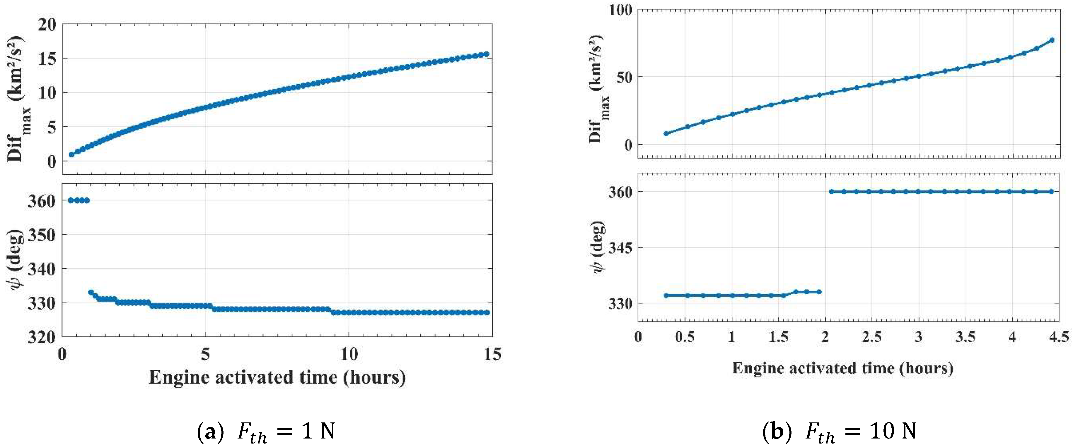
Figure 9). Based on these facts,
Figure 14 shows a summary of the maximum efficiency of the maneuver and its respective
, for
,
and
.
It is evident from
Figure 14a that, when
, the maneuver needs more propulsion time to reach the maximum
(~15 km
2/s
2), but it is still smaller than the results shown in
Figure 14b, which reaches its maximum (~77 km
2/s
2) with approximately 4.42 h of active propulsion. Another observation is that, for the situation where the smaller force is applied to the spacecraft (
) and the propulsion acts for up to approximately 0.9 h, the maximum efficiency of the maneuver occurs for the initial condition
, the region with no variation of energy coming from gravity. In this propulsion time, the values of
for
range between 327° and 332°, following a decreasing pattern. When
,
ranges around 332° when the engine works for up to approximately two hours and, above that,
is 360°. The trajectories for the SBCT maneuvers for maximum
conditions are shown in
Figure 15.
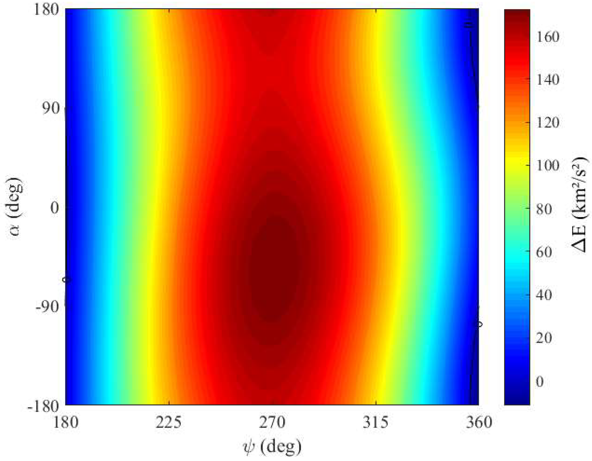
5. Direction of the Thrust
The next step is to study the effects of the direction of the thrust. To undertake this, we mapped the energy variations for the largest energy gains, because this is the best case. From the previous analyzes for
, we know that the best efficiencies in energy gains for the SBCT maneuver occur for larger distances from the periapsis and larger propulsion arcs. It can also be seen that these best efficiency regions are located in the regions where the angle of approach obtains energy gains from gravity. Then, we fixed these values and mapped the effect of the variations of the direction of the thrust in the energy variations of the maneuver. It is well known that the angle of approach has very important effects on the results.
Figure 16 shows the variations of energy for each angle of approach and the direction of the thrust.
Note that the regions of energy reductions are small when
and
; that
for
; and that
for
and
. Once again,
for
. Both cases occur in angles of approach where the gravity does not change the energy of the spacecraft. Therefore, the non-zero variations of energy are a consequence of the thrust, which works to maximize the gain or minimize the loss of energy. However, in the cases where
, the variations in the direction and magnitude of the thrust were not enough to reverse the loss. All other results on the map show energy gains, with the largest energy variation conditions around
and approximately
, as highlighted in
Figure 17 and
Figure 18. Still looking at the general map of solutions (
Figure 16), we can see that the effect of
is smaller when compared to the effects of
, appearing in smooth curves.
In
Figure 17, we compare the maximum energy variations (
) and their respective directions of the thrust (
) for each angle of approach (
) with the PSB data, where PSB represents the powered Swing-By maneuver, which is the pure maneuver combined with a single impulse applied at the periapsis [
9], and with the unpowered Swing-By maneuver [
5] under the same initial conditions. In this way we can undertake a better analysis of the effects of the variations of the direction of the thrust. For this analysis (
Figure 17) and
Figure 18, whose solutions were obtained numerically, we fitted the numerical results to obtain an empirical equation for the largest energy gains as a function of the variations of the direction of the thrust and angle of approach. The purpose of these equations is to provide a quick and approximate visualization of the solutions.
The largest differences between given by the SBCT and PSB maneuver, obtained from numerical studies, is approximately 11.63 km2/s2, and it occurs around , when (SBCT) and (PSB).
Equations (9)–(13) were obtained from the fitting of the numerical results obtained in the present work. The
for SBCT obtained by numerical solutions (dashed black curve in
Figure 17a), with
and
varying in steps of 1.0°, can be approximated by a fitted curve of the numerical data (continuous orange curve,
Figure 17a) by Equation (9), for the initial conditions adopted and
.
Note that, from this equation, it is also possible to quantify the maximum variations of energy for whose curve was hidden here because , in this case, represents the smallest energy loss.
This fitted equation allows the fast and approximate calculation of the maximum energy variation. Regarding both methods of calculation, the largest
are shown in
Table 2. It is clear that the approximations are very good.
Relative to the directions of the propulsion, it increases from
to
(continuous black curve,
Figure 17b); that is, the thruster has a component pointing towards the secondary body. The differences in
of the SBCT and PSB is that, in the case of PSB, it follows the analysis of [
9], using an impulse that accelerates the spacecraft and sends it towards the celestial body. For the SBCT, where the thrust is continuous for a long period of time, there is a balance between propulsion and gravity to obtain the best results for the maneuver, so
is needed to attend the whole maneuver. In situations where
, the spacecraft is decelerated, increasing the curvature of its trajectory, and bringing it as close as possible to the body, so it takes more advantage of gravity to gain energy. For
(when it crosses
), gravity already has a greater effect on the spacecraft, since the maximum gain occurs for
[
9], so the spacecraft takes advantage of the thrust to accelerate more, since the thruster has a component in the direction of the motion of the spacecraft. Equation (10) gives
from the fitting data (continuous orange curve,
Figure 17b), for
.
For the interval
, where the gravity works to remove energy from the spacecraft,
increases from 0° to 180° to move the spacecraft away from the body and to reduce the effect of gravity. Its behavior can be approximated by Equation (11).
It is also possible to analyze the best energy variation and angle of approach for each direction of the thrust when the objective is to increase the energy of the spacecraft. Note, in
Figure 18a, that the largest energy gains for the continuous maneuver when compared to the one-impulsive maneuver, occurs for directions of the thrust approximately between −147° and 32°, i.e., there is a component of the thrust towards the secondary body. It can also be seen that the largest maximum energy variation occurs for
.
The approximate equation for the maximum variations of energy (
) for SBCT are obtained by fitting the numerical data from the simulations (continuous orange curve,
Figure 18a), when
(Equation (13)) and
is given by Equation (12).
For the maximum angle of approach (
) the approximate equation is given by Equation (13).
For the magnitude of the thrust adopted in
Section 5, that is,
; the one-impulsive PSB maneuver with thrust applied in the periapsis has the maximum approach angle (
) at exactly
in all directions of the thrust, as shown by the continuous blue line in
Figure 18b. This behavior corroborates what is explained in Reference [
5], and it also shows that the gravitational effect dominates the impulsive maneuver in this situation. For SBCT with
i.e., no more than exactly 270°, and for all values of
, the direction and magnitude of the thrust are working together to find a balance with the gravitational effect.
6. Conclusions
The present paper is a study measuring the variations of energy given by a maneuver that combines the application of a continuous thrust with a close approach to a celestial body. The main goal was to obtain the differences in energy variations when applying the continuous thrust during the closest approach or far from it. To do that, we defined the “efficiency” of the maneuver that uses the continuous thrust during the close encounter of the spacecraft with the secondary body, and then we compared those results with the maneuver that makes the pure gravity close approach far from the continuous thrust maneuver. Using this technique, we can quantify the extra energy obtained by the spacecraft by applying the thrust during the closest approach as a function of the parameters involved in the maneuver.
To show the results, we plotted color maps showing the efficiency of the SBCT maneuver. Those plots identify the regions where each maneuver (SBCT and the SB plus CT) gives more energy to the spacecraft.
The SBCT maneuver can also be used for many goals, like close observations of the secondary body, passages by given regions, etc. Therefore, the cost–benefit of the fuel consumption is not the only criterion to be observed, and several missions can use this technique, even if it is more expensive in terms of fuel consumption.
The results show that the SBCT maneuver is efficient, for the energy gain, at , and that this efficiency tends to be larger for around 360°, a region where the effect of gravity on the energy variation tends to be smaller (for , ). Of course, if the goal is to gain energy, other values for the angle of approach are better, but they may not be possible to achieve due to other constraints of the trajectory. On the other hand, the pure maneuver (SB) with propulsion applied at a point distant from (CT) is more efficient for all cases where (Equation (8)) is less than zero, in addition to greater than zero and . This occurs due to a combination of the turning angle generated by the combined maneuver, which defines the energy gains from gravity, and the energy given directly by the propulsion system. It is also noted that larger values for the periapsis radius () give more importance to the propulsive part of the maneuver, since the farther from the celestial body the spacecraft passes, the smaller the effect of gravity.
Regarding the propulsive part of the maneuver, the greater the thrust (
), the greater the energy gain in the SBCT, as expected, but we also see that the efficiency also increases. In the case of continuous thrust and short propulsion arcs, we considered that the duration of the propulsion is equals to the SB, using the parameter
to define it. The results showed that the higher the
, in these conditions, the larger the efficiency. For higher thrust and shorter times,
defines only the SB and “
” defines the propulsion arc. The results showed that there is a limit between the combination of
and
(
Figure 9) where, after that, there are occurrences of captures, collisions or singularities due to the maneuver. We also showed the conditions for maximum efficiency and quantified the active propellant time based on the data obtained.
Regarding the direction of the thrust, we map the best maximum energy gains, when and around 270°, taking into account that gives a component of the thrust that sends the spacecraft to the direction of the secondary body, taking increased advantage of gravity. The results also show maximum gains for close to 360° (region of greater efficiency when compared to the SB plus CT maneuver). In both cases, the SBCT maneuver is also more efficient than PSB one-impulse maneuver (with the impulse applied at the periapsis). The ideal magnitude of varies according to the positioning of the periapsis () in the orbit, so that a balance can be achieved between the gains due to gravity and propulsion.
Those mappings are important to describe the limitations and real gains of the SBCT and to uncover the ideal initial conditions according to the objectives of the mission. Approximate equations for the maximum energy variations and their respective directions of the thrust and approach angle were also presented. They were obtained from the fitting of numerical data obtained from simulations and can be used to facilitate the study by making fast calculations.
This study can be applicable to other systems, in addition to the Sun–Jupiter system presented here and can be used for missions that need the extra energy given by the combined maneuver or that have constraints which require the use of continuous thrust and close approach maneuvers.

 ,
, 


