Two-Dimensional Turbulent Thermal Free Jet: Conservation Laws, Associated Lie Symmetry and Invariant Solutions ^†

Abstract

The two-dimensional turbulent thermal free jet is formulated in the boundary layer approximation using the Reynolds averaged momentum balance equation and the averaged energy balance equation. The turbulence is described by Prandtl’s mixing length model for the eddy viscosity ${\nu }_T$ with mixing length l and eddy thermal conductivity ${\kappa }_T$ with mixing length $l_{\theta }$. Since ${\nu }_T$ and ${\kappa }_T$ are proportional to the mean velocity gradient the momentum and thermal boundaries of the flow coincide. The conservation laws for the system of two partial differential equations for the stream function of the mean flow and the mean temperature difference are derived using the multiplier method. Two conserved vectors are obtained. The conserved quantities for the mean momentum and mean heat fluxes are derived. The Lie point symmetry associated with the two conserved vectors is derived and used to perform the reduction of the partial differential equations to a system of ordinary differential equations. It is found that the mixing lengths l and $l_{\theta }$ are proportional. A turbulent thermal jet with ${\nu }_T\ne 0$ and ${\kappa }_T\ne 0$ but vanishing kinematic viscosity $\nu$ and thermal conductivity $\kappa$ is studied. Prandtl’s hypothesis that the mixing length is proportional to the width of the jet is made to complete the system of equations. An analytical solution is derived. The boundary of the jet is determined with the aid of a conserved quantity and found to be finite. Analytical solutions are derived and plotted for the streamlines of the mean flow and the lines of constant mean thermal difference. The solution differs from the analytical solution obtained in the limit $\nu \to 0$ and $\kappa \to 0$ without making the Prandtl’s hypothesis. For $\nu \ne 0$ and $\kappa \ne 0$ a numerical solution is derived using a shooting method with the two conserved quantities as targets instead of boundary conditions. The numerical solution is verified by comparing it to the analytical solution when $\nu \to 0$ and $\kappa \to 0$. Because of the limitations imposed by the accuracy of any numerical method the numerical solution could not reliably determine if the jet is unbounded when $\nu \ne 0$ and $\kappa \ne 0$ but for large distance from the centre line, $\nu >{\nu }_T$ and $\kappa >{\kappa }_T$ and the jet behaves increasingly like a laminar jet which is unbounded. The streamlines of the mean flow and the lines of constant mean temperature difference are plotted for $\nu =0$ and $\kappa =0$.

1. Introduction

Turbulent thermal jets have many engineering applications which include propulsion in aircraft and boiler furnaces [1] and heating and drying of surfaces [2]. In this paper, Lie symmetry methods and conservation laws for partial differential equations will be applied to investigate the two-dimensional turbulent thermal jet.

Over the decades, numerical [3,4], analytical [5,6,7] and experimental studies have been carried out [8,9,10]. Howarth [5] gave an analytical treatment to the two-dimensional and axisymmetric turbulent thermal free jets using Prandtl mixing lengths to model the eddy viscosity and eddy thermal conductivity. He showed using a similarity argument that the mixing lengths are proportional to the distance from the nozzle along the centre line of the jet. He also showed that the temperature distribution is similar to the velocity distribution. Hinze and Van der Heggezijnen [10] compared the analytical results of Howarth [5] with experimental data. Sforza and Mons [8] presented analytical and experimental investigations of mass, momentum and thermal transfer of a radial turbulent thermal free jet. The authors used an extension by Baron and Alexander [6] of Reichardt’s inductive theory of turbulence [7] to close the Reynolds averaged equations. They compared their analytical results with experimental data. The analytical results derived in [5,8] neglect the kinematic viscosity and thermal conductivity. This is a reasonable physical assumption since the eddy viscosity and eddy thermal conductivity are large compared to the kinematic viscosity and thermal conductivity.

In this paper, the turbulence will be described by an eddy viscosity in the Reynolds averaged momentum balance equation and by an eddy thermal conductivity in the averaged energy balance equation. The eddy viscosity is described by Prandtl’s mixing length model and the eddy conductivity is modelled using a thermal mixing length. We assume the momentum and thermal mixing lengths are functions only of the distance from the nozzle along the centre line of the jet. The form of the functions will be determined by the invariance condition that the system of partial differential equations describing the turbulent thermal jet admit a Lie point symmetry. In general a jet is laminar in a short region close to the nozzle, but is turbulent further downstream. In the fully developed region, a turbulent model is required.

When expressed in terms of the stream function the two-dimensional turbulent thermal free jet is described by a coupled system of two partial differential equations. An invariant solution will be investigated by using conservation laws and Lie group analysis for partial differential equations. Several methods can be used to derive conservation laws for partial differential Equations [11]. We will use the multiplier method. The homogeneous boundary conditions of a jet are not sufficient to determine the invariant solution. Conserved quantities are needed which are obtained by integrating conservation laws across the jet and using the boundary conditions. For each conservation law there is a conserved vector. The Lie point symmetry associated with the conserved vector is derived by using a result due to Kara and Mahomed [12,13]. The order of the prolongation required in the derivation of an associated Lie point symmetry is one less than when the full Lie point symmetry is derived. The system of two partial differential equations for the turbulent thermal free jet is reduced to a system of two ordinary differential equations. When the reduction is performed by an associated Lie point symmetry the ordinary differential equations can be integrated at least once by the double reduction theorem of Sjoberg [14,15].

This approach to the derivation of an invariant solution was taken by Mason and Hill [16] who considered an axisymmetric turbulent jet described by an eddy viscosity which depends only on position. It was also applied by Magan et al. [17,18] to the two-dimensional free jet and liquid jet of a non-Newtonian power law fluid and by Hutchinson [19] to the turbulent far wake with variable mainstream flow. A new feature of the problem is the system of two coupled partial differential equations and two mixing lengths, Prandtl’s mixing length and the thermal mixing length.

Although the kinematic viscosity, $\nu$, and the thermal conductivity, $\kappa$, are small compared with the eddy kinematic viscosity, ${\nu }_T$, and the eddy thermal conductivity, ${\kappa }_T$, in a real fluid they are non-zero and can play a significant part in the mathematical solution. We will consider two cases:

(i)

$\nu$ and $\kappa$ are neglected, $\nu =0$ and $\kappa =0$,

(ii)

$\nu$ and $\kappa$ are retained, $\nu \ne 0$ and $\kappa \ne 0$.

When $\nu \ne 0$ and $\kappa \ne 0$ it is found that the associated Lie point symmetry and mixing lengths are fully determined. When $\nu =0$ and $\kappa =0$ a further equation is needed to determine completely the associated Lie point symmetry. We will use for this condition Prandtl’s hypothesis [20] that the mixing length is proportional to the breadth of the jet.

When $\nu \ne 0$ and $\kappa \ne 0$ we solve the reduced ordinary differential equations numerically. A shooting method is used to convert the boundary value problem to an initial value problem [21]. The two conserved quantities are the targets for the shooting method. Mason and Hill [16] applied a shooting method that used one conserved quantity for the target. The partial derivatives are approximated using a secant method which is an adaption of the method by Edun and Akanabi [22] for two variables. The numerical method is verified by confirming that the numerical solution for the x and y components of the fluid velocity, shear stress and temperature difference tends to the analytical solution as $\nu \to 0$ and $\kappa \to 0$.

The research questions are:

(i)

What are the assumptions and conditions in the boundary layer approximation for the two-dimensional thermal jet?

(ii)

What are the conservation laws and conserved vectors for the partial differential equations and what are the conserved quantities for the two-dimensional turbulent thermal free jet?

(iii)

What is the Lie point symmetry associated with the conserved vectors?

(iv)

How do the momentum and thermal mixing lengths depend on the distance from the orifice along the centre line of the jet?

(v)

Under what conditions is the turbulent thermal jet bounded in the transverse direction to the flow and what is the equation of the boundary?

(vi)

Can analytical solutions for the stream function and mean temperature difference be derived for $\nu =0$, $\kappa =0$, and numerical solutions using the shooting method for $\nu \ne 0$, $\kappa \ne 0$?

(vii)

Does the numerical solution for $\nu \to 0$, $\kappa \to 0$ agree with the analytical solution for $\nu =0$, $\kappa =0$.

(viii)

Can analytical solutions for the streamlines of the mean flow and the lines of constant mean temperature difference be derived and plotted for $\nu =0$, $\kappa =0$?

The paper is organised as follows: In Section 2, the two-dimensional turbulent free jet is formulated mathematically. In Section 3, conservation laws for the system of two partial differential equations describing the turbulent jet are derived using the multiplier method and two conserved quantities are obtained. The associated Lie point symmetry is derived in Section 4 and the general form of the invariant solution is obtained in Section 5. In Section 6, analytical solutions for $\nu =0$ and $\kappa =0$ and a numerical solution for $\nu \ne 0$ and $\kappa \ne 0$ are found. We discuss the results in Section 7 and finally the conclusions are summarised in Section 8.

2. Mathematical Formulation

Consider a two-dimensional thermal turbulent free jet. The fluid emerges from a long narrow orifice in a wall. The fluid is viscous and incompressible and is the same as the surrounding fluid which is at rest far from the jet. The x-axis is along the centre line of the plane of the mean flow of the jet and the y-axis is perpendicular to the x-axis as shown in Figure 1.

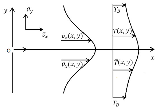
Figure 1. Schematic diagram of the mean velocity and the mean temperature profiles of a two-dimensional thermal turbulent free jet.

2.1. Averaged Momentum and Energy Balance Equations

In the turbulent thermal jet, the fluid velocity, pressure and temperature consist of a mean and a fluctuation:

$$\begin{array}{cccc}\hfill v_x(x,y,t)& ={\overline{v}}_x(x,y)+v_x^{\prime }(x,y,t),\hfill & \hfill \hspace{1em}\hspace{1em}{v}_y(x,y,t)& ={\overline{v}}_y(x,y)+v_y^{\prime }(x,y,t),\hfill \end{array}$$

(1)

$$\begin{array}{ccc}\hfill p(x,y,t)& =\overline{p}(x,y)+p^{\prime }(x,y,t),\hfill & \hfill \hspace{1em}\hspace{1em}T(x,y,t)=\overline{T}(x,y)+T^{\prime }(x,y,t),\end{array}$$

(2)

where p is the pressure, T is the temperature of the fluid and $v_x$ and $v_y$ are the x and y components of the velocity, respectively. The mean of a quantity $f(x,y,t)$ is defined by

$$\overline{f}(x,y)=\frac{1}{N}{\int }_{t-\frac{1}{2}N}^{t+\frac{1}{2}N}f(x,y,\tau )d\tau ,$$

(3)

where it is assumed that the time interval N can be chosen sufficiently large that the mean is independent of time. Flows in which it is assumed that the mean flow is independent of time are referred to as steady turbulent flows [23].

Substituting the decomposition (1) into the continuity equation of an incompressible fluid for a two-dimensional flow and taking the time average gives

$$\frac{\partial {\overline{v}}_x}{\partial x}+\frac{\partial {\overline{v}}_y}{\partial y}=0,$$

(4)

$$\frac{\partial v_x^{\prime }}{\partial x}+\frac{\partial v_y^{\prime }}{\partial y}=0.$$

(5)

Substituting the decompositions (1) and (2) into the Navier–Stokes equation and the energy balance equation for a two-dimensional flow and taking the time average gives

$$\begin{array}{c}\rho \left[{\overline{v}}_x\frac{\partial {\overline{v}}_x}{\partial x}+{\overline{v}}_y\frac{\partial {\overline{v}}_x}{\partial y}\right]=-\frac{\partial \overline{p}}{\partial x}+\frac{\partial }{\partial x}\left[\mu \left(\frac{\partial {\overline{v}}_x}{\partial x}+\frac{\partial {\overline{v}}_x}{\partial x}\right)-\rho \overline{v_x^{\prime }{v}_x^{\prime }}\right]+\frac{\partial }{\partial y}\left[\mu \left(\frac{\partial {\overline{v}}_x}{\partial y}+\frac{\partial {\overline{v}}_y}{\partial x}\right)-\rho \overline{v_x^{\prime }{v}_y^{\prime }}\right],\end{array}$$

(6)

$$\begin{array}{c}\rho \left[{\overline{v}}_x\frac{\partial {\overline{v}}_y}{\partial x}+{\overline{v}}_y\frac{\partial {\overline{v}}_y}{\partial y}\right]=-\frac{\partial \overline{p}}{\partial y}+\frac{\partial }{\partial x}\left[\mu \left(\frac{\partial {\overline{v}}_x}{\partial y}+\frac{\partial {\overline{v}}_y}{\partial x}\right)-\rho \overline{v_y^{\prime }{v}_x^{\prime }}\right]+\frac{\partial }{\partial y}\left[\mu \left(\frac{\partial {\overline{v}}_y}{\partial y}+\frac{\partial {\overline{v}}_y}{\partial y}\right)-\rho \overline{v_y^{\prime }{v}_y^{\prime }}\right],\end{array}$$

(7)

$$\begin{array}{c}\rho c_v\left[{\overline{v}}_x\frac{\partial \overline{T}}{\partial x}+{\overline{v}}_y\frac{\partial \overline{T}}{\partial y}\right]=\frac{\partial }{\partial x}\left[\kappa \frac{\partial \overline{T}}{\partial x}-\rho c_v\overline{v_x^{\prime }{T}^{\prime }}\right]+\frac{\partial }{\partial y}\left[\kappa \frac{\partial \overline{T}}{\partial y}-\rho c_v\overline{v_y^{\prime }{T}^{\prime }}\right],\end{array}$$

(8)

where $\rho$, $\mu$, $c_v$ and $\kappa$ are constants and are the density, coefficient of viscosity, specific heat capacity at constant volume and the coefficient of thermal conductivity of the fluid. The mean velocity and the fluctuation separately satisfy the continuity equation. Equations (6) and (7) are the x- and y-components of the Reynolds averaged Navier–Stokes equation and (8) is the averaged energy balance equation. In Equation (8), the average rate of dissipation of energy due to viscosity is neglected. It can be neglected for small velocities because it is proportional to the square of the velocity [24].

Now by the Boussinesq hypothesis the turbulent Reynolds stresses, $-\rho \overline{v_i^{\prime }{v}_j^{\prime }}$, are related to the rate of strain tensor of the mean flow by [23]

$$-\rho \overline{v_i^{\prime }{v}_j^{\prime }}=-\frac{2}{3}\rho k{\delta }_{ij}+{\mu }_T\left(\frac{\partial {\overline{v}}_i}{\partial x_j}+\frac{\partial {\overline{v}}_j}{\partial x_i}\right)$$

(9)

where ${\mu }_T$ is the eddy or turbulent viscosity,

$$k=\frac{1}{2}\overline{v_i^{\prime }{v}_i^{\prime }}$$

(10)

and k is the mean kinetic energy of the fluctuations per unit mass. It is readily verified with the aid of (4) that the trace of the left and right hand sides of (9) are equal. Furthermore, in analogy with Fourier’s law of heat conduction [24],

$$\rho c_v\overline{v_i^{\prime }{T}^{\prime }}=-{\kappa }_T\frac{\partial \overline{T}}{\partial x_i},$$

(11)

where ${\kappa }_T$ is the eddy or turbulent thermal conductivity. Equations (6) to (8) become

$$\begin{array}{c}\rho \left[{\overline{v}}_x\frac{\partial {\overline{v}}_x}{\partial x}+{\overline{v}}_y\frac{\partial {\overline{v}}_x}{\partial y}\right]=-\frac{\partial }{\partial x}\left(\overline{p}+\frac{2}{3}\rho k\right)+\frac{\partial }{\partial x}\left[\left(\mu +{\mu }_T\right)\left(\frac{\partial {\overline{v}}_x}{\partial x}+\frac{\partial {\overline{v}}_x}{\partial x}\right)\right]\\ +\frac{\partial }{\partial y}\left[\left(\mu +{\mu }_T\right)\left(\frac{\partial {\overline{v}}_x}{\partial y}+\frac{\partial {\overline{v}}_y}{\partial x}\right)\right],\end{array}$$

(12)

$$\begin{array}{c}\rho \left[{\overline{v}}_x\frac{\partial {\overline{v}}_y}{\partial x}+{\overline{v}}_y\frac{\partial {\overline{v}}_y}{\partial y}\right]=-\frac{\partial }{\partial y}\left(\overline{p}+\frac{2}{3}\rho k\right)+\frac{\partial }{\partial x}\left[\left(\mu +{\mu }_T\right)\left(\frac{\partial {\overline{v}}_x}{\partial y}+\frac{\partial {\overline{v}}_y}{\partial x}\right)\right]\\ +\frac{\partial }{\partial y}\left[\left(\mu +{\mu }_T\right)\left(\frac{\partial {\overline{v}}_y}{\partial y}+\frac{\partial {\overline{v}}_y}{\partial y}\right)\right],\end{array}$$

(13)

$$\begin{array}{c}\rho c_v\left[{\overline{v}}_x\frac{\partial \overline{T}}{\partial x}+{\overline{v}}_y\frac{\partial \overline{T}}{\partial y}\right]=\frac{\partial }{\partial x}\left[\left(\kappa +{\kappa }_T\right)\frac{\partial \overline{T}}{\partial x}\right]+\frac{\partial }{\partial y}\left[\left(\kappa +{\kappa }_T\right)\frac{\partial \overline{T}}{\partial y}\right].\end{array}$$

(14)

Unlike $\mu$ and $\kappa$ which are properties of the fluid, ${\mu }_T$ and ${\kappa }_T$ are properties of the flow. The sums $\mu +{\mu }_T$ and $\kappa +{\kappa }_T$ are referred to as the effective viscosity and the effective thermal conductivity.

2.2. Boundary Layer Theory

The application of boundary layer theory does not require a solid boundary. It applies to fluid flows with regions of rapid change in the fluid variables. In two-dimensional turbulent jet flow there are rapid changes in the mean fluid variables in the region of the centre line in the direction perpendicular to the centre line. We will outline briefly turbulent thermal boundary layer theory for the mean flow, defining carefully the turbulent Reynolds and Prandtl numbers and highlighting the approximations made.

Let $U_0$ and L be the characteristic velocity and characteristic length in the x-direction. For the jet, $U_0$ can be chosen as the mean fluid velocity at the nozzle and L the distance over which the mean fluid velocity along the centre line decreases significantly. Let $P_0$ be the characteristic value of the modified fluid pressure $\overline{p}+\frac{2}{3}\rho k$, ${\delta }_V$ be the characteristic length in the y-direction for changes in the mean fluid velocity and modified pressure and ${\delta }_{\theta }$ be the characteristic length in the y-direction for changes in the mean temperature. The characteristic quantities $P_0$, ${\delta }_V$ and ${\delta }_{\theta }$ will be determined in the course of the analysis. A star denotes a variable made dimensionless by division by its characteristic value. Let V be the characteristic value of the mean fluid velocity in the y-direction. Then the conservation of mass equation for the mean flow, (4), in dimensionless form is

$$\frac{\partial {\overline{v}}_x^{*}}{\partial x^{*}}+\frac{V}{U}\frac{L}{{\delta }_V}\frac{\partial {\overline{v}}_y^{*}}{\partial y^{*}}=0.$$

(15)

Equation (15) cannot be approximated because mass is always conserved. The two terms in (15) must therefore balance and

$$V=\frac{{\delta }_V}{L}U.$$

(16)

The effective kinematic viscosity is

$${\nu }_E=\frac{1}{\rho }\left(\mu +{\mu }_T\right)=\nu +{\nu }_T.$$

(17)

The characteristic kinematic eddy viscosity and eddy thermal conductivity are denoted by ${\nu }_{TC}$ and ${\kappa }_{TC}$.

Equations (12) to (14) in dimensionless form are

$$\begin{array}{c}{\overline{v}}_x^{*}\frac{\partial {\overline{v}}_x^{*}}{\partial x^{*}}+{\overline{v}}_y^{*}\frac{\partial {\overline{v}}_x^{*}}{\partial y^{*}}=-\frac{P_0}{\rho U_0^2}\frac{\partial }{\partial x^{*}}\left({\overline{p}}^{*}+\frac{2}{3}\rho k^{*}\right)+\frac{2}{Re\left(T\right)}\frac{\partial }{\partial x^{*}}\left[\left(\frac{\nu +{\nu }_T}{\nu +{\nu }_{TC}}\right)\frac{\partial {\overline{v}}_x^{*}}{\partial x^{*}}\right]\\ +\frac{1}{Re\left(T\right)}{\left(\frac{L}{{\delta }_V}\right)}^2\frac{\partial }{\partial y^{*}}\left[\left(\frac{\nu +{\nu }_T}{\nu +{\nu }_{TC}}\right)\left(\frac{\partial {\overline{v}}_x^{*}}{\partial y^{*}}+{\left(\frac{{\delta }_V}{L}\right)}^2\frac{\partial {\overline{v}}_y^{*}}{\partial x^{*}}\right)\right],\end{array}$$

(18)

$$\begin{array}{c}{\left(\frac{{\delta }_V}{L}\right)}^2\left[{\overline{v}}_x^{*}\frac{\partial {\overline{v}}_y^{*}}{\partial x^{*}}+{\overline{v}}_y^{*}\frac{\partial {\overline{v}}_y^{*}}{\partial y^{*}}\right]=-\frac{P_0}{\rho U_0^2}\frac{\partial }{\partial y^{*}}\left({\overline{p}}^{*}+\frac{2}{3}\rho k^{*}\right)+\frac{1}{Re\left(T\right)}\frac{\partial }{\partial x^{*}}\left[\left(\frac{\nu +{\nu }_T}{\nu +{\nu }_{TC}}\right)\left(\frac{\partial {\overline{v}}_x^{*}}{\partial y^{*}}+{\left(\frac{{\delta }_V}{L}\right)}^2\frac{\partial {\overline{v}}_y^{*}}{\partial x^{*}}\right)\right]\\ +\frac{2}{Re\left(T\right)}\frac{\partial }{\partial y^{*}}\left[\left(\frac{\nu +{\nu }_T}{\nu +{\nu }_{TC}}\right)\frac{\partial {\overline{v}}_y^{*}}{\partial y^{*}}\right],\end{array}$$

(19)

$$\begin{array}{c}{\overline{v}}_x^{*}\frac{\partial {\overline{T}}^{*}}{\partial x^{*}}+\frac{{\delta }_V}{{\delta }_{\theta }}{\overline{v}}_y^{*}\frac{\partial {\overline{T}}^{*}}{\partial y^{*}}=\frac{1}{Pr\left(T\right)Re\left(T\right)}\frac{\partial }{\partial x^{*}}\left[\left(\frac{\kappa +{\kappa }_T}{\kappa +{\kappa }_{TC}}\right)\frac{\partial {\overline{T}}^{*}}{\partial x^{*}}\right]\\ +\frac{1}{Pr\left(T\right)Re\left(T\right)}{\left(\frac{L}{{\delta }_{\theta }}\right)}^2\frac{\partial }{\partial y^{*}}\left[\left(\frac{\kappa +{\kappa }_T}{\kappa +{\kappa }_{TC}}\right)\frac{\partial {\overline{T}}^{*}}{\partial y^{*}}\right],\end{array}$$

(20)

where

$$\begin{array}{cccc}\hfill Re\left(T\right)& =\frac{U_{0}L}{\nu +{\nu }_{TC}},\hfill & \hfill Pr\left(T\right)& =\frac{\rho c_v}{\left(\kappa +{\kappa }_{TC}\right)}\left(\nu +{\nu }_{TC}\right).\hfill \end{array}$$

(21)

We have defined the turbulent Reynolds number and turbulent Prandtl number in terms of the effective kinematic viscosity and the effective thermal conductivity. The Prandtl number is the ratio of the viscous diffusion rate to the thermal diffusion rate.

Consider first Equation (18). The pressure gradient plays an essential role in a fluid flow and cannot be neglected. We therefore insist that the gradient of the modified pressure balance the inertia term and require that

$$P_0=\rho U_0^2.$$

(22)

In the boundary layer the rapid rate of change of ${\overline{v}}_x$ with y should be sufficient to prevent the viscous term in (18) from being negligible [25]. We therefore choose

$$\frac{{\delta }_V}{L}=\frac{1}{\sqrt{Re\left(T\right)}}.$$

(23)

Consider next Equation (20). The rapid rate of change of the mean temperature $\overline{T}$ with y in the boundary layer should be just sufficient to prevent the thermal conduction term from being negligible. Thus

$$\frac{{\delta }_{\theta }}{L}=\frac{1}{\sqrt{Pr\left(T\right)}\sqrt{Re\left(T\right)}}.$$

(24)

From (23) and (24),

$$\frac{{\delta }_V}{{\delta }_{\theta }}=\sqrt{Pr\left(T\right)}.$$

(25)

Equations (18) to (20) become

$$\begin{array}{c}{\overline{v}}_x^{*}\frac{\partial {\overline{v}}_x^{*}}{\partial x^{*}}+{\overline{v}}_y^{*}\frac{\partial {\overline{v}}_x^{*}}{\partial y^{*}}=-\frac{\partial }{\partial x^{*}}\left({\overline{p}}^{*}+\frac{2}{3}\rho k^{*}\right)+\frac{2}{Re\left(T\right)}\frac{\partial }{\partial x^{*}}\left[\left(\frac{\nu +{\nu }_T}{\nu +{\nu }_{TC}}\right)\frac{\partial {\overline{v}}_x^{*}}{\partial x^{*}}\right]\\ +\frac{\partial }{\partial y^{*}}\left[\left(\frac{\nu +{\nu }_T}{\nu +{\nu }_{TC}}\right)\left(\frac{\partial {\overline{v}}_x^{*}}{\partial y^{*}}+\frac{1}{Re\left(T\right)}\frac{\partial {\overline{v}}_y^{*}}{\partial x^{*}}\right)\right],\end{array}$$

(26)

$$\begin{array}{c}\frac{1}{Re\left(T\right)}\left[{\overline{v}}_x^{*}\frac{\partial {\overline{v}}_y^{*}}{\partial x^{*}}+{\overline{v}}_y^{*}\frac{\partial {\overline{v}}_y^{*}}{\partial y^{*}}\right]=-\frac{\partial }{\partial y^{*}}\left({\overline{p}}^{*}+\frac{2}{3}\rho k^{*}\right)+\frac{1}{Re\left(T\right)}\frac{\partial }{\partial x^{*}}\left[\left(\frac{\nu +{\nu }_T}{\nu +{\nu }_{TC}}\right)\left(\frac{\partial {\overline{v}}_x^{*}}{\partial y^{*}}+\frac{1}{Re\left(T\right)}\frac{\partial {\overline{v}}_y^{*}}{\partial x^{*}}\right)\right]\\ +\frac{2}{Re\left(T\right)}\frac{\partial }{\partial y^{*}}\left[\left(\frac{\nu +{\nu }_T}{\nu +{\nu }_{TC}}\right)\frac{\partial {\overline{v}}_y^{*}}{\partial y^{*}}\right],\end{array}$$

(27)

$$\begin{array}{c}{\overline{v}}_x^{*}\frac{\partial {\overline{T}}^{*}}{\partial x^{*}}+\sqrt{Pr\left(T\right)}{\overline{v}}_y^{*}\frac{\partial {\overline{T}}^{*}}{\partial y^{*}}=\frac{1}{Pr\left(T\right)Re\left(T\right)}\frac{\partial }{\partial x^{*}}\left[\left(\frac{\kappa +{\kappa }_T}{\kappa +{\kappa }_{TC}}\right)\frac{\partial {\overline{T}}^{*}}{\partial y^{*}}\right]+\frac{\partial }{\partial y^{*}}\left[\left(\frac{\kappa +{\kappa }_T}{\kappa +{\kappa }_{TC}}\right)\frac{\partial {\overline{T}}^{*}}{\partial y^{*}}\right].\end{array}$$

(28)

Now for a viscous boundary layer and a thermal boundary layer,

$$\begin{array}{cccc}\hfill \frac{{\delta }_V}{L}& =\frac{1}{\sqrt{Re\left(T\right)}}<<1,\hfill & \hfill \hspace{1em}\hspace{1em}\hspace{1em}\frac{{\delta }_{\theta }}{L}& =\frac{1}{\sqrt{Pr\left(T\right)Re\left(T\right)}}<<1.\hfill \end{array}$$

(29)

We will consider the case in which $Pr\left(T\right)$ is order of magnitude unity. Then from (25) the effective widths of the viscous and thermal boundary layers, ${\delta }_V$ and ${\delta }_{\theta }$, are the same order of magnitude. Neglecting terms of order $1/Re\left(T\right)$ and reverting to original variables, Equations (26) to (28) reduce to

$${\overline{v}}_x\frac{\partial {\overline{v}}_x}{\partial x}+{\overline{v}}_y\frac{\partial {\overline{v}}_x}{\partial y}=-\frac{1}{\rho }\frac{\partial }{\partial x}\left(\overline{p}+\frac{2}{3}\rho k\right)+\frac{\partial }{\partial y}\left[\left(\nu +{\nu }_T\right)\frac{\partial {\overline{v}}_x}{\partial y}\right],$$

(30)

$$\begin{array}{c}\frac{\partial }{\partial y}\left(\overline{p}+\frac{2}{3}\rho k\right)=0,\end{array}$$

(31)

$$\rho c_v\left({\overline{v}}_x\frac{\partial \overline{T}}{\partial x}+{\overline{v}}_y\frac{\partial \overline{T}}{\partial y}\right)=\frac{\partial }{\partial y}\left[\left(\kappa +{\kappa }_T\right)\frac{\partial \overline{T}}{\partial y}\right].$$

(32)

From (31) the modified pressure is independent of y. Since the modified pressure depends only on x it equals the pressure, $p\left(x\right)$, in the laminar mainstream flow:

$$\overline{p}+\frac{2}{3}\rho k=p\left(x\right).$$

(33)

However, the mainstream flow is inviscid. Euler’s equation therefore applies and

$$\frac{dp}{dx}=-\rho U\frac{dU}{dx}=0$$

(34)

since for a jet the mainstream velocity $U\left(x\right)$ is zero. Equation (30) becomes

$${\overline{v}}_x\frac{\partial {\overline{v}}_x}{\partial x}+{\overline{v}}_y\frac{\partial {\overline{v}}_x}{\partial y}=\frac{\partial }{\partial y}\left[\left(\nu +{\nu }_T\right)\frac{\partial {\overline{v}}_x}{\partial y}\right].$$

(35)

The boundary layer equations for a two-dimensional turbulent jet are (4), (32) and (35).

2.3. Eddy Viscosity and Eddy Thermal Conductivity

From Prandtl’s mixing length model for the eddy viscosity [23,25],

$${\nu }_T=l^2\left|\frac{\partial {\overline{v}}_x}{\partial y}\right|,$$

(36)

where l is Prandtl’s mixing length. This model applies for parallel mean flow and for a two-dimensional turbulent boundary layer for which $\partial {\overline{v}}_y/\partial x$ can be neglected.

The eddy thermal conductivity, ${\kappa }_T$, is derived using dimensional analysis. It is assumed that the component of the turbulent heat flux vector depends on the $xy$-component of the Reynolds stress tensor, the y-component of the spatial gradient of the mean temperature and on a thermal mixing length. It is found that [24]

$$\frac{{\kappa }_T}{\rho c_v}=l{l}_{\theta }\left|\frac{\partial {\overline{v}}_x}{\partial y}\right|,$$

(37)

where $l_{\theta }$ is the thermal mixing length.

The mixing length is generally independent of the velocity. We will assume that the mixing lengths depend only on x,

$$\begin{array}{ccc}\hfill l& =l\left(x\right),\hfill & \hfill l_{\theta }=l_{\theta }\left(x\right).\end{array}$$

(38)

We will consider the upper half of the jet. In this region, ${\overline{v}}_x(x,y)$ is a decreasing function of y and

$$\left|\frac{\partial {\overline{v}}_x}{\partial y}\right|=-\frac{\partial {\overline{v}}_x}{\partial y},y>0.$$

(39)

The boundary layer Equations (32) and (35) become

$${\overline{v}}_x\frac{\partial {\overline{v}}_x}{\partial x}+{\overline{v}}_y\frac{\partial {\overline{v}}_x}{\partial y}=\frac{\partial }{\partial y}\left[\left(\nu -l^2\left(x\right)\frac{\partial {\overline{v}}_x}{\partial y}\right)\frac{\partial {\overline{v}}_x}{\partial y}\right],$$

(40)

$${\overline{v}}_x\frac{\partial \overline{T}}{\partial x}+{\overline{v}}_y\frac{\partial \overline{T}}{\partial y}=\frac{\partial }{\partial y}\left[\left(\frac{\kappa }{\rho c_v}-l\left(x\right)l_{\theta }\left(x\right)\frac{\partial {\overline{v}}_x}{\partial y}\right)\frac{\partial \overline{T}}{\partial y}\right].$$

(41)

The mixing lengths, $l\left(x\right)$ and $l_{\theta }\left(x\right)$, will be determined from the condition that partial differential Equations (40) and (41) admit an invariant solution.

2.4. Boundary Conditions for the Upper Half of The Jet

Consider first the boundary conditions on the centre line, $y=0$. Since the jet is symmetrical about the centre line and there is no cavity formation, ${\overline{v}}_y$ vanishes at $y=0$ and ${\overline{v}}_x$ and $\overline{T}$ are maximum at $y=0$. Hence

$$\begin{array}{ccccccc}\hfill y& =0:\hfill & \hfill \hspace{1em}\hspace{1em}{\overline{v}}_y(x,0)& =0,\hfill & \hfill \hspace{1em}\hspace{1em}\frac{\partial {\overline{v}}_x}{\partial y}(x,0)& =0,\hfill & \hfill \hspace{1em}\hspace{1em}\frac{\partial \overline{T}}{\partial y}(x,0)=0.\end{array}$$

(42)

From (36) and (37), ${\nu }_T$ and ${\kappa }_T$ both vanish on the curve $y=y_B\left(x\right)$ where $y_B\left(x\right)$ satisfies

$$\frac{\partial \overline{v}}{\partial y}(x,y_B\left(x\right))=0.$$

(43)

The boundary of the turbulent thermal jet in the upper half of the $xy$-plane is therefore $y=y_B\left(x\right)$ and the range of the jet is $-y_B\left(x\right)\le y\le y_B\left(x\right)$. The boundary $y=y_B\left(x\right)$ may be a finite curve $y_B\left(x\right)$ may be infinite for all $0\le x<\infty$. We shall investigate the solution for two cases.

Case (a), $\nu =0$ and $\kappa =0$

Since $\nu <<{\nu }_T$ and $\kappa <<{\kappa }_T$ we make the approximation that $\nu =0$ and $\kappa =0$. Outside the turbulent jet, $y_B\left(x\right)<y<\infty$, the fluid is inviscid, not heat conducting and at rest with constant ambient temperature $T_B$ where

$$T_B=\overline{T}(x,y_B\left(x\right)).$$

(44)

Tangential mean velocities match at the boundary. Thus, from Figure 2a,

$$\begin{array}{cccc}\hfill y& =y_B\left(x\right):\hfill & \hfill \hspace{1em}\hspace{1em}\hspace{1em}{\overline{v}}_x(x,y_B\left(x\right))cos\alpha +{\overline{v}}_y(x,y_B\left(x\right))sin\alpha & =0\hfill \end{array}$$

(45)

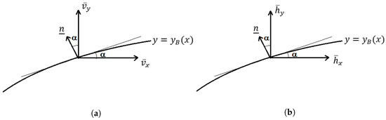
Figure 2. Schematic diagram of a flux through the boundary of the jet. (a) Momentum flux, (b) Thermal flux.

Expressing (45) in dimensionless variables and neglecting terms order ${\delta }_V/L$ we obtain the boundary condition

$${\overline{v}}_x(x,y_B\left(x\right))=0.$$

(46)

The normal component of the turbulent heat flux vector vanishes at the boundary. However,

$${\overline{h}}_i=-\left(\kappa +{\kappa }_T\right)\frac{\partial \overline{T}}{\partial x_i}$$

(47)

and since ${\kappa }_T=0$ on the boundary and $\kappa =0$, ${\overline{h}}_i=0$ and the boundary condition is satisfied identically.

Case (b), $\nu \ne 0$ and $\kappa \ne 0$

For a real fluid, although $\nu$ and $\kappa$ may be small they are never zero. In boundary layer theory, the flow in the boundary layer is matched to a mainstream with $\nu =0$ and $\kappa =0$. We do that here. The boundary condition (46) is again imposed. The normal component of the heat flux vector vanishes at the boundary. Thus, from Figure 2b,

$$\begin{array}{cccc}\hfill y& =y_B\left(x\right):\hfill & \hfill {\overline{h}}_{y}cos\alpha -{\overline{h}}_{x}sin\alpha & =0\hfill \end{array}$$

(48)

and using (47) with ${\kappa }_T=0$ on the boundary

$$\begin{array}{cccc}\hfill y& =y_B\left(x\right):\hfill & \hfill -\kappa \frac{\partial \overline{T}}{\partial y}cos\alpha +\kappa \frac{\partial \overline{T}}{\partial x}sin\alpha & =0.\hfill \end{array}$$

(49)

Expressing (49) in dimensionless variables and neglecting terms of order ${\delta }_{\theta }/L$, since $\kappa \ne 0$, we obtain the boundary condition

$$\begin{array}{cccccc}\hfill y& =y_B\left(x\right):\hfill & \hfill \frac{\partial \overline{T}}{\partial y}(x,y_B\left(x\right))& =0,\hfill & \hfill \kappa & \ne 0.\hfill \end{array}$$

(50)

Since the mean flow is two-dimensional and incompressible a stream function $\psi (x,y)$ can be introduced defined by

$$\begin{array}{ccc}\hfill {\overline{v}}_x& =\frac{\partial \psi }{\partial y},\hfill & \hfill {\overline{v}}_y=-\frac{\partial \psi }{\partial x}.\end{array}$$

(51)

The conservation of mass equation for the mean flow, (4), is identically satisfied. We formulate the problem in terms of the mean temperature difference, $S(x,y)$, instead of the mean temperature where

$$S(x,y)=\overline{T}(x,y)-T_B$$

(52)

where $T_B$, defined by (44), is a constant. Equations (40) and (41) become

$$\frac{\partial \psi }{\partial y}\frac{{\partial }^2\psi }{\partial x\partial y}-\frac{\partial \psi }{\partial x}\frac{{\partial }^2\psi }{\partial y^2}=\frac{\partial }{\partial y}\left[\left(\nu -l^2\left(x\right)\frac{{\partial }^2\psi }{\partial y^2}\right)\frac{{\partial }^2\psi }{\partial y^2}\right],$$

(53)

$$\frac{\partial \psi }{\partial y}\frac{\partial S}{\partial x}-\frac{\partial \psi }{\partial x}\frac{\partial S}{\partial y}=\frac{\partial }{\partial y}\left[\left(\frac{\kappa }{\rho c_v}-l\left(x\right)l_{\theta }\left(x\right)\frac{{\partial }^2\psi }{\partial y^2}\right)\frac{\partial S}{\partial y}\right].$$

(54)

The boundary conditions are

$$\begin{array}{cccccccc}\hfill y& =0:\hfill & \hfill \frac{\partial \psi }{\partial x}(x,0)& =0,\hfill & \hfill \frac{{\partial }^2\psi }{\partial y^2}(x,0)& =0,\hfill & \hfill \frac{\partial S}{\partial y}(x,0)& =0,\hfill \end{array}$$

(55)

$$\begin{array}{cccccccc}\hfill y& =y_B\left(x\right):\hfill & \hfill \frac{\partial \psi }{\partial y}(x,y_B\left(x\right))& =0,\hfill & \hfill \frac{{\partial }^2\psi }{\partial y^2}(x,y_B\left(x\right))& =0,\hfill & \hfill S(x,y_B\left(x\right))& =0,\hfill \end{array}$$

(56)

and when $\kappa \ne 0$,

$$\frac{\partial S}{\partial y}(x,y_B\left(x\right))=0.$$

(57)

3. Conservation Laws and Conserved Quantities

3.1. Conservation Laws

In jet flow problems conserved quantities are required to complete the solution. The boundary conditions (55) and (56), which are all homogeneous, do not specify the strength of the jet. We will derive the conserved quantities for the turbulent thermal jet in a systematic way by first finding the conservation laws for the system of partial differential Equations (53) and (54).

When working with conservation laws and Lie point symmetries, x, y, $\psi$, S and all the partial derivatives of $\psi$ and S with respect to x and y are regarded as independent variables and the subscript-notation is used for partial differentiation. Thus, $x,y,\psi ,S,{\psi }_x,{\psi }_y,S_x,S_y$ and all higher partial derivatives with respect to x and y are independent variables. The notation $\frac{\partial \psi }{\partial x}$, $\frac{{\partial }^{2}S}{\partial x\partial y}$,... is used when $\psi$ and S are regarded as functions of independent variables x and y. Equations (53) and (54) in subscript notation are

$${\psi }_y{\psi }_{xy}-{\psi }_x{\psi }_{yy}-\nu {\psi }_{yyy}+2l^2\left(x\right){\psi }_{yy}{\psi }_{yyy}=0,$$

(58)

$${\psi }_y{S}_x-{\psi }_x{S}_y-\frac{\kappa }{\rho c_v}{S}_{yy}+l\left(x\right)l_{\theta }\left(x\right)\left({\psi }_{yy}{S}_{yy}+{\psi }_{yyy}{S}_y\right)=0.$$

(59)

A conservation law for the system of partial differential Equations (58) and (59) is defined by

$$D_1{T}^1+D_2{T}^2{|}_{\left(58\right),\left(59\right)}=0,$$

(60)

where

$$D_1=D_x=\frac{\partial }{\partial x}+{\psi }_x\frac{\partial }{\partial \psi }+S_x\frac{\partial }{\partial S}+{\psi }_{xx}\frac{\partial }{\partial {\psi }_x}+{\psi }_{yx}\frac{\partial }{\partial {\psi }_y}+S_{xx}\frac{\partial }{\partial S_x}+S_{yx}\frac{\partial }{\partial S_y}+\cdots ,$$

(61)

$$D_2=D_y=\frac{\partial }{\partial y}+{\psi }_y\frac{\partial }{\partial \psi }+S_y\frac{\partial }{\partial S}+{\psi }_{xy}\frac{\partial }{\partial {\psi }_x}+{\psi }_{yy}\frac{\partial }{\partial {\psi }_y}+S_{xy}\frac{\partial }{\partial S_x}+S_{yy}\frac{\partial }{\partial S_y}+\cdots .$$

(62)

and $T^1$, $T^2$ are the components of the conserved vector $T=(T^1,T^2)$. We will use the multiplier method to derive the conservation laws [11]. Multipliers ${\mathsf{\Lambda }}_1$ and ${\mathsf{\Lambda }}_2$ are determined which satisfy

$$\begin{array}{c}{\mathsf{\Lambda }}_1\left({\psi }_y{\psi }_{xy}-{\psi }_x{\psi }_{yy}-\nu {\psi }_{yyy}+2l^2\left(x\right){\psi }_{yy}{\psi }_{yyy}\right)+\\ {\mathsf{\Lambda }}_2({\psi }_y{S}_x-{\psi }_x{S}_y-\frac{\kappa }{\rho c_v}{S}_{yy}+l\left(x\right)l_{\theta }\left(x\right){\psi }_{yy}{S}_{yy}+l\left(x\right)l_{\theta }\left(x\right){\psi }_{yyy}{S}_y)=D_x{T}^1+D_y{T}^2\end{array}$$

(63)

for all functions $\psi (x,y)$ and $S(x,y)$. Once ${\mathsf{\Lambda }}_1$ and ${\mathsf{\Lambda }}_2$ have been determined we will impose the conditions (58) and (59) on (63). We will take

$$\begin{array}{cccc}\hfill {\mathsf{\Lambda }}_1& ={\mathsf{\Lambda }}_1(x,y,\psi ,S),\hfill & \hfill {\mathsf{\Lambda }}_2& ={\mathsf{\Lambda }}_2(x,y,\psi ,S).\hfill \end{array}$$

(64)

Partial derivatives of $\psi$ and S could be included in ${\mathsf{\Lambda }}_1$ and ${\mathsf{\Lambda }}_2$ to investigate higher order conservation laws but it is sufficient to consider multipliers of the form (64) to obtain conserved vectors needed for the turbulent thermal jet.

We apply the standard Euler operators $E_{\psi }$ and $E_S$ defined by

$$E_{\psi }=\frac{\partial }{\partial \psi }-D_x\frac{\partial }{\partial {\psi }_x}-D_y\frac{\partial }{\partial {\psi }_y}+D_x^2\frac{\partial }{\partial {\psi }_{xx}}+D_x{D}_y\frac{\partial }{\partial {\psi }_{xy}}+D_y^2\frac{\partial }{\partial {\psi }_{yy}}-D_y^3\frac{\partial }{\partial {\psi }_{yyy}}-\cdots$$

(65)

and

$$E_S=\frac{\partial }{\partial S}-D_x\frac{\partial }{\partial S_x}-D_y\frac{\partial }{\partial S_y}+D_x^2\frac{\partial }{\partial S_{xx}}+D_x{D}_y\frac{\partial }{\partial S_{xy}}+D_y^2\frac{\partial }{\partial S_{yy}}-D_y^3\frac{\partial }{\partial S_{yyy}}-\cdots$$

(66)

to Equation (63) to obtain determining equations for ${\mathsf{\Lambda }}_1$ and ${\mathsf{\Lambda }}_2$. The Euler operators annihilate the divergence expression on the right hand side of (63). Thus

$$\begin{array}{c}E\left[\phantom{\frac{\kappa }{\rho c_v}}{\mathsf{\Lambda }}_1\left({\psi }_y{\psi }_{xy}-{\psi }_x{\psi }_{yy}-\nu {\psi }_{yyy}+2l^2\left(x\right){\psi }_{yy}{\psi }_{yyy}\right)+\right.\\ \left.{\mathsf{\Lambda }}_2({\psi }_y{S}_x-{\psi }_x{S}_y-\frac{\kappa }{\rho c_v}{S}_{yy}+l\left(x\right)l_{\theta }\left(x\right){\psi }_{yy}{S}_{yy}+l\left(x\right)l_{\theta }\left(x\right){\psi }_{yyy}{S}_y)\right]=0,\end{array}$$

(67)

where we set $E=E_{\psi }$ and $E=E_S$ in turn.

We first expand (67) with $E=E_S$. Since (63) is satisfied for all functions $\psi (x,y)$ and $S(x,y)$ we can equate to zero the coefficients of the independent partial derivatives of $\psi$ and S in the expansion (67). Hence extracting the terms in (67) which depend on ${\psi }_x$ gives

$$\begin{array}{cccc}\hfill {\mathsf{\Lambda }}_1& ={\mathsf{\Lambda }}_1(x,y,\psi ),\hfill & \hfill {\mathsf{\Lambda }}_2& ={\mathsf{\Lambda }}_2(x,\psi ,S).\hfill \end{array}$$

(68)

The terms which depend on ${\psi }_y{\psi }_{yyy}$ and $S_y{\psi }_{yyy}$ yield ${\mathsf{\Lambda }}_2={\mathsf{\Lambda }}_2\left(x\right)$ and the coefficient of ${\psi }_y$ gives ${\mathsf{\Lambda }}_2=c_2$ where $c_2$ is a constant. Hence

$$\begin{array}{cccc}\hfill {\mathsf{\Lambda }}_1& ={\mathsf{\Lambda }}_1(x,y,\psi ),\hfill & \hfill {\mathsf{\Lambda }}_2& =c_2.\hfill \end{array}$$

(69)

We next expand (67) with $E=E_{\psi }$ and ${\mathsf{\Lambda }}_1$ and ${\mathsf{\Lambda }}_2$ given by (69). The coefficient of $c_2$ vanishes so that the expansion depends only on the partial derivatives of $\psi$. Separating according to the partial derivatives of $\psi$ we find that

$$\begin{array}{cccc}\hfill {\mathsf{\Lambda }}_1& =c_1,\hfill & \hfill {\mathsf{\Lambda }}_2& =c_2,\hfill \end{array}$$

(70)

where $c_1$ is a constant.

Substituting Equation (70) into (63) and rearranging terms gives

$$\begin{array}{c}{D}_x\left[c_1{\psi }_y^2+c_2{\psi }_{y}S\right]+D_y\left[c_1\left(-{\psi }_x{\psi }_y-\nu {\psi }_{yy}+l^2\left(x\right){\psi }_{yy}^2\right)+c_2\left(-\frac{\kappa }{\rho c_v}{S}_y-{\psi }_{x}S+l\left(x\right)l_{\theta }\left(x\right){\psi }_{yy}{S}_y\right)\right]\\ =D_x{T}^1+D_y{T}^2\end{array}$$

(71)

for arbitrary functions $\psi (x,y)$ and $S(x,y)$. When $\psi (x,y)$ and $S(x,y)$ are solutions of the system of Equations (58) and (59) then (71) becomes

$$\begin{array}{c}{D}_x\left[c_1{\psi }_y^2+c_2{\psi }_{y}S\right]\\ +D_y\left[\phantom{\frac{\kappa }{\rho c_v}}{c}_1\left(-{\psi }_x{\psi }_y-\nu {\psi }_{yy}+l^2\left(x\right){\psi }_{yy}^2\right)+c_2\left(-\frac{\kappa }{\rho c_v}{S}_y-{\psi }_{x}S+l\left(x\right)l_{\theta }\left(x\right){\psi }_{yy}{S}_y\right)\right]{|}_{\left(58\right),\left(59\right)}=0.\end{array}$$

(72)

Thus, any conserved vector of the system of partial differential Equations (58) and (59) with multipliers ${\mathsf{\Lambda }}_1(x,y,\psi ,S)$ and ${\mathsf{\Lambda }}_2(x,y,\psi ,S)$ is a linear combination of the following two conserved vectors:

$c_1=1$ and $c_2=0$: $T_{\left(1\right)}=(T^1,T^2)$

$$\begin{array}{cccc}\hfill T^1& ={\psi }_y^2,\hfill & \hfill T^2& =-{\psi }_x{\psi }_y-\nu {\psi }_{yy}+l^2\left(x\right){\psi }_{yy}^2.\hfill \end{array}$$

(73)

$c_1=0$ and $c_2=1$: $T_{\left(2\right)}=(T^1,T^2)$

$$\begin{array}{cccc}\hfill T^1& ={\psi }_{y}S,\hfill & \hfill T^2& =-\frac{\kappa }{\rho c_v}{S}_y-{\psi }_{x}S+l\left(x\right)l_{\theta }\left(x\right){\psi }_{yy}{S}_y.\hfill \end{array}$$

(74)

The vector $\rho T_{\left(1\right)}$ is the momentum flux conserved vector and $\rho c_v{T}_{\left(2\right)}$ is the thermal flux conserved vector.

3.2. Conserved Quantities

To obtain conserved quantities we integrate the conservation law (72) with respect to y from $y=0$ to $y=y_B\left(x\right)$ and impose boundary conditions (55) to (57).

3.2.1. Conserved Quantity Derived from the Momentum Flux Conserved Vector

We now treat $T^1$ and $T^2$ as functions of the independent variables x and y. Then

$$D_x{T}^1+D_y{T}^2=\frac{\partial T^1}{\partial x}(x,y)+\frac{\partial T^2}{\partial y}(x,y).$$

(75)

Therefore the conserved vectors with x and y regarded as independent variables satisfy

$$\frac{\partial T^1}{\partial x}\left(x,y\right)+\frac{\partial T^2}{\partial y}\left(x,y\right)=0.$$

(76)

Hence the conserved vector with components (73) satisfies

$$\frac{\partial }{\partial x}\left[{\left(\frac{\partial \psi }{\partial y}\right)}^2\right]+\frac{\partial }{\partial y}\left[-\frac{\partial \psi }{\partial x}\frac{\partial \psi }{\partial y}-\nu \frac{{\partial }^2\psi }{\partial y^2}+l^2\left(x\right){\left(\frac{{\partial }^2\psi }{\partial y^2}\right)}^2\right]=0.$$

(77)

Then integrating (77) with respect to y from $y=0$ to $y=y_B\left(x\right)$ and using the formula for differentiation under the integral sign [26] gives

$$\begin{array}{c}\frac{d}{dx}{\int }_0^{y_B\left(x\right)}{\left(\frac{\partial \psi }{\partial y}\right)}^{2}dy-\frac{d{y}_B}{dx}{\left(\frac{\partial \psi }{\partial y}(x,y_B\left(x\right))\right)}^2+\left[-\frac{\partial \psi }{\partial x}\frac{\partial \psi }{\partial y}-\nu \frac{{\partial }^2\psi }{\partial y^2}+l^2\left(x\right){\left(\frac{{\partial }^2\psi }{\partial y^2}\right)}^2\right]{|}_{y=0}^{y=y_B\left(x\right)}=0.\end{array}$$

(78)

Imposing boundary conditions (55) and (56) the second and third terms of (78) vanish. Hence (78) reduces to

$$\begin{array}{c}\frac{d}{dx}{\int }_0^{y_B\left(x\right)}{\left(\frac{\partial \psi }{\partial y}(x,y)\right)}^{2}dy=0.\end{array}$$

(79)

Therefore

$$J=2\rho {\int }_0^{y_B\left(x\right)}{\left(\frac{\partial \psi }{\partial y}(x,y)\right)}^{2}dy$$

(80)

is a constant independent of x. The constant J is the flux in the x-direction of the x-component of the momentum of the jet and is the strength of the jet.

3.2.2. Conserved Quantity Derived from the Thermal Flux Conserved Vector

Substituting the conserved vector components (74) into (76) gives

$$\frac{\partial }{\partial x}\left(S\frac{\partial \psi }{\partial y}\right)+\frac{\partial }{\partial y}\left(l\left(x\right)l_{\theta }\left(x\right)\frac{{\partial }^2\psi }{\partial y^2}\frac{\partial S}{\partial y}-\frac{\kappa }{\rho c_v}\frac{\partial S}{\partial y}-S\frac{\partial \psi }{\partial x}\right)=0.$$

(81)

Again, integrating (81) with respect to y from $y=0$ to $y=y_B\left(x\right)$ and using the formula for differentiation under the integral sign [26] gives

$$\begin{array}{c}\frac{d}{dx}{\int }_0^{y_B\left(x\right)}S(x,y)\frac{\partial \psi }{\partial y}(x,y)dy-\frac{d{y}_B}{dx}S(x,y_B\left(x\right))\frac{\partial \psi }{\partial y}(x,y_B\left(x\right))\\ +\left[l\left(x\right)l_{\theta }\left(x\right)\frac{{\partial }^2\psi }{\partial y^2}\frac{\partial S}{\partial y}-\frac{\kappa }{\rho c_v}\frac{\partial S}{\partial y}-S\frac{\partial \psi }{\partial x}\right]{|}_{y=0}^{y=y_B\left(x\right)}=0.\end{array}$$

(82)

Imposing boundary conditions (55) to (57) Equation (82) reduces to

$$\frac{d}{dx}{\int }_0^{y_B\left(x\right)}S(x,y)\frac{\partial \psi }{\partial y}(x,y)dy=0.$$

(83)

Hence

$$K=2\rho c_v{\int }_0^{y_B\left(x\right)}S(x,y)\frac{\partial \psi }{\partial y}(x,y)dy$$

(84)

is a constant independent of x. The constant K is the power per unit area of the jet.

The conserved quantities J and K apply for $\nu \ne 0$, $\kappa \ne 0$ and for $\nu =0$, $\kappa =0$. Together they characterise the strength of the thermal jet.

4. Associated Lie Point Symmetry

We will derive the Lie point symmetry X associated with both the momentum flux conserved vector (73) and the thermal flux conserved vector (74).

The Lie point symmetry

$$X={\xi }^1(x,y,\psi ,S)\frac{\partial }{\partial x}+{\xi }^2(x,y,\psi ,S)\frac{\partial }{\partial y}+{\eta }^1(x,y,\psi ,S)\frac{\partial }{\partial \psi }+{\eta }^2(x,y,\psi ,S)\frac{\partial }{\partial S}$$

(85)

is said to be associated with the conserved vector $T=(T^1,T^2)$ provided [12]

$$X^{[\infty ]}\left(T^i\right)+T^i{D}_k\left({\xi }^k\right)-T^k{D}_k\left({\xi }^i\right)=0,i=1,2$$

(86)

where $X^{[\infty ]}$ denotes the prolongation of X to as many orders as required depending on the partial derivatives in T. The two components in (86) can be expressed as

$$X^{[\infty ]}\left(T^1\right)+T^1{D}_y\left({\xi }^2\right)-T^2{D}_y\left({\xi }^1\right)=0,$$

(87)

$$X^{[\infty ]}\left(T^2\right)+T^2{D}_x\left({\xi }^1\right)-T^1{D}_x\left({\xi }^2\right)=0.$$

(88)

Because of the form of the conserved vectors, (73) and (74),

$$X^{[\infty ]}=X+{\zeta }_1^1\frac{\partial }{\partial {\psi }_x}+{\zeta }_2^1\frac{\partial }{\partial {\psi }_y}+{\zeta }_{22}^1\frac{\partial }{\partial {\psi }_{yy}}+{\zeta }_2^2\frac{\partial }{\partial S_y}$$

(89)

where

$$\begin{array}{cccc}\hfill {\zeta }_i^{\alpha }& =D_i\left({\eta }^{\alpha }\right)-u_k^{\alpha }{D}_i\left({\xi }^k\right),\hfill & \hfill {\zeta }_{ij}^{\alpha }& =D_i\left({\zeta }_j^{\alpha }\right)-u_{ik}^{\alpha }{D}_j\left({\xi }^k\right)\hfill \end{array}$$

(90)

and $x^1=x$, $x^2=y$, $u^1=\psi$ and $u^2=S$.

4.1. Association with the Momentum Flux Conserved Vector

The conserved vector is given by (73). Expanding Equation (87) and splitting it into the coefficients of the powers and products of the first order partial derivatives ${\psi }_x$, ${\psi }_y$ and $S_y$ we find that

$$\begin{array}{cccccccc}\hfill {\xi }^1& ={\xi }^1\left(x\right),\hfill & \hfill {\xi }^2& ={\xi }^2(x,y),\hfill & \hfill {\eta }^1& ={\eta }^1(x,\psi ),\hfill & \hfill {\eta }^2& ={\eta }^2(x,y,\psi ,S).\hfill \end{array}$$

(91)

provided

$$2\frac{\partial {\eta }^1}{\partial \psi }(x,\psi )-\frac{\partial {\xi }^2}{\partial y}(x,y)=0.$$

(92)

Differentiating (92) with respect to y gives

$${\xi }^2(x,y)=a_1\left(x\right)y+a_2\left(x\right),$$

(93)

where $a_1\left(x\right)$ and $a_2\left(x\right)$ are arbitrary functions of x. Substituting (93) back into (92) and integrating with respect to $\psi$ gives

$${\eta }^1(x,\psi )=\frac{1}{2}{a}_1\left(x\right)\psi +a_3\left(x\right),$$

(94)

where $a_3\left(x\right)$ is an arbitrary function of x. Because ${\xi }^1={\xi }^1\left(x\right)$ the remaining terms in (87) are identically zero. Hence (87) yields

$$\begin{array}{ccccccc}\hfill {\xi }^1& ={\xi }^1\left(x\right),\hfill & \hfill {\xi }^2(x,y)& =a_1\left(x\right)y+a_2\left(x\right),\hfill & \hfill {\eta }^1(x,\psi )& =\frac{1}{2}{a}_1\left(x\right)\psi +a_3\left(x\right),\hfill & \hfill {\eta }^2={\eta }^2(x,y,\psi ,S).\end{array}$$

(95)

Equation (95) is valid for all values of $\nu$ and $\kappa$.

Expanding the second component (88) we find that it depends only on the partial derivatives of $\psi$. Splitting (88) into the coefficients of the independent partial derivatives of $\psi$ we obtain the determining equations

$$\begin{array}{cccc}\hfill {\psi }_y:\frac{1}{2}\frac{d{a}_1}{dx}\psi +\frac{d{a}_3}{dx}& =0,\hfill & \hfill {\psi }_{yy}:\nu \left(\frac{d{\xi }^1}{dx}-\frac{3}{2}{a}_1\left(x\right)\right)& =0,\hfill \end{array}$$

(96)

$${\left({\psi }_{yy}\right)}^2:l^2\left(x\right)\frac{d{\xi }^1}{dx}+2l\left(x\right)\frac{dl}{dx}\left(x\right){\xi }^1-3l^2\left(x\right)a_1\left(x\right)=0.$$

(97)

Further separating the first equation of (96) by $\psi$ gives that $a_1$ and $a_3$ are constants.

Associating the Lie point symmetry (85) with the momentum flux conserved vector (74) therefore yields

$$\begin{array}{cccccccc}\hfill {\xi }^1& ={\xi }^1\left(x\right),\hfill & \hfill {\xi }^2(x,y)& =a_{1}y+a_2\left(x\right),\hfill & \hfill {\eta }^1\left(\psi \right)& =\frac{1}{2}{a}_1\psi +a_3,\hfill & \hfill {\eta }^2& ={\eta }^2(x,y,\psi ,S),\hfill \end{array}$$

(98)

provided

$$\begin{array}{cccc}\hfill \nu \left(\frac{d{\xi }^1}{dx}-\frac{3}{2}{a}_1\right)& =0,\hfill & \hfill \frac{d{\xi }^1}{dx}+\frac{2}{l\left(x\right)}\frac{dl}{dx}\left(x\right){\xi }^1\left(x\right)& =3a_1.\hfill \end{array}$$

(99)

4.2. Association with the Thermal Conserved Vector

The conserved vector is given by (74). Using (98) and the conserved vector (74), Equation (87) reduces to

$${\eta }^2\left(S\right)=-\frac{1}{2}{a}_{1}S.$$

(100)

Finally expanding (88) and separating the equation into the coefficients of the independent partial derivatives of $\psi$ and S we obtain the determining equations

$$S_y:\frac{\kappa }{\rho c_v}\left(\frac{d{\xi }^1}{dx}-\frac{3}{2}{a}_1\right)=0,$$

(101)

$${\psi }_{yy}{S}_y:\frac{d{\xi }^1}{dx}l\left(x\right)l_{\theta }\left(x\right)+{\xi }^1\left(x\right)\frac{d}{dx}\left(l\left(x\right)l_{\theta }\left(x\right)\right)-3a_{1}l\left(x\right)l_{\theta }\left(x\right)=0.$$

(102)

By associating the Lie point symmetry (85) with the momentum and thermal flux conserved vectors, (73) and (74), we found that

$$\begin{array}{cccccccc}\hfill {\xi }^1& ={\xi }^1\left(x\right),\hfill & \hfill {\xi }^2(x,y)& =a_{1}y+a_2\left(x\right),\hfill & \hfill {\eta }^1\left(\psi \right)& =\frac{1}{2}{a}_1\psi +a_3,\hfill & \hfill {\eta }^2\left(S\right)& =-\frac{1}{2}{a}_{1}S\hfill \end{array}$$

(103)

provided

$$\begin{array}{cccc}\hfill \nu \left(\frac{d{\xi }^1}{dx}-\frac{3}{2}{a}_1\right)& =0,\hfill & \hfill \kappa \left(\frac{d{\xi }^1}{dx}-\frac{3}{2}{a}_1\right)& =0,\hfill \end{array}$$

(104)

$$\frac{d{\xi }^1}{dx}+\frac{2}{l\left(x\right)}\frac{dl}{dx}\left(x\right){\xi }^1\left(x\right)=3a_1,$$

(105)

$$\frac{d{\xi }^1}{dx}l\left(x\right)l_{\theta }\left(x\right)+{\xi }^1\left(x\right)\frac{d}{dx}\left(l\left(x\right)l_{\theta }\left(x\right)\right)-3a_{1}l\left(x\right)l_{\theta }\left(x\right)=0.$$

(106)

4.3. Mixing Lengths

Consider first Equations (105) and (106). Replacing $\frac{d{\xi }^1}{dx}$ in (106) using (105), Equation (106) reduces to

$$\frac{1}{l_{\theta }}\frac{d{l}_{\theta }}{dx}=\frac{1}{l}\frac{dl}{dx}$$

(107)

and therefore

$$l_{\theta }\left(x\right)=Dl\left(x\right)$$

(108)

where D is a constant. The two mixing lengths are proportional and this is satisfied for both $\nu =0$, $\kappa =0$ and $\nu \ne 0$, $\kappa \ne 0$.

Consider $\nu \ne 0$ and $\kappa \ne 0$. The two equations in (104) are compatible and give

$$\frac{d{\xi }^1}{dx}=\frac{3}{2}{a}_1.$$

(109)

Hence

$${\xi }^1\left(x\right)=\frac{3}{2}{a}_{1}x+a_4$$

(110)

where $a_4$ is a constant. Substituting (110) for ${\xi }^1\left(x\right)$ into (105) we obtain

$$\frac{1}{l}\frac{dl}{dx}=\frac{3a_1}{4\left(\frac{3}{2}{a}_{1}x+a_4\right)}$$

(111)

and therefore

$$l\left(x\right)=A_1{\left(\frac{3}{2}{a}_{1}x+a_4\right)}^{\frac{1}{2}}$$

(112)

where $A_1$ is a constant.

In summary when $\nu \ne 0$ and $\kappa \ne 0$, the Lie point symmetry associated with the conserved vectors (73) and (74) is

$$X=\left(\frac{3}{2}{a}_{1}x+a_4\right)\frac{\partial }{\partial x}+\left(a_{1}y+a_2\left(x\right)\right)\frac{\partial }{\partial y}+\left(\frac{1}{2}{a}_1\psi +a_3\right)\frac{\partial }{\partial \psi }-\frac{1}{2}{a}_{1}S\frac{\partial }{\partial S}$$

(113)

and

$$\begin{array}{cccc}\hfill l\left(x\right)& =A_1{\left(\frac{3}{2}{a}_{1}x+a_4\right)}^{\frac{1}{2}},\hfill & \hfill l_{\theta }\left(x\right)& =A_2{\left(\frac{3}{2}{a}_{1}x+a_4\right)}^{\frac{1}{2}},\hfill \end{array}$$

(114)

where $A_2$ is a constant. When $\nu =0$ and $\kappa =0$,

$$X={\xi }^1\left(x\right)\frac{\partial }{\partial x}+\left(a_{1}y+a_2\left(x\right)\right)\frac{\partial }{\partial y}+\left(\frac{1}{2}{a}_1\psi +a_3\right)\frac{\partial }{\partial \psi }-\frac{1}{2}{a}_{1}S\frac{\partial }{\partial S}$$

(115)

and

$$\begin{array}{cccc}\hfill l_{\theta }\left(x\right)& =Dl\left(x\right),\hfill & \hfill \frac{d{\xi }^1}{dx}+\frac{2}{l\left(x\right)}\frac{dl}{dx}{\xi }^1& =3a_1.\hfill \end{array}$$

(116)

When $\nu \ne 0$ and $\kappa \ne 0$ the associated Lie point symmetry and mixing lengths are determined except for the constants $a_1$, $a_3$, $a_4$, $A_1$ and $A_2$ and the function $a_2\left(x\right)$. When $\nu =0$ and $\kappa =0$, ${\xi }^1\left(x\right)$ is not determined but it is related to $l\left(x\right)$ through the second equation of (116) and $l_{\theta }\left(x\right)$ is proportional to $l\left(x\right)$.

5. Invariant Solutions

The form of the invariant solution depends on whether $\nu \ne 0$ and $\kappa \ne 0$ or $\nu =0$ and $\kappa =0$. We will consider the general case in which $a_1\ne 0$.

5.1. Case$\nu \ne 0$ and $\kappa \ne 0$.

Let

$$\begin{array}{cccccccccc}\hfill c_1& =\frac{2}{3}\frac{a_4}{a_1},\hfill & \hfill c_2\left(x\right)& =\frac{2}{3}\frac{a_2\left(x\right)}{a_1},\hfill & \hfill c_3& =\frac{2}{3}\frac{a_3}{a_1},\hfill & \hfill l_1& ={\left(\frac{3a_1}{2}\right)}^{\frac{1}{2}}{A}_1,\hfill & \hfill l_2& ={\left(\frac{3a_1}{2}\right)}^{\frac{1}{2}}{A}_2.\hfill \end{array}$$

(117)

Then the Lie point symmetry (113) and the mixing lengths (114) become

$$X=(x+c_1)\frac{\partial }{\partial x}+\left(\frac{2}{3}y+c_2\left(x\right)\right)\frac{\partial }{\partial y}+\left(\frac{1}{3}\psi +c_3\right)\frac{\partial }{\partial \psi }-\frac{1}{3}S\frac{\partial }{\partial S},$$

(118)

$$\begin{array}{cccc}\hfill l\left(x\right)& =l_1{(x+c_1)}^{\frac{1}{2}},\hfill & \hfill l_{\theta }\left(x\right)& =l_2{\left(x+c_1\right)}^{\frac{1}{2}}.\hfill \end{array}$$

(119)

Then $\psi =f(x,y)$ and $S=g(x,y)$ are invariant solutions of the system of partial differential Equations (53) and (54) provided

$$X(\psi -f(x,y)){|}_{\psi =f(x,y)}=0,$$

(120)

$$X(S-g(x,y)){|}_{S=g(x,y)}=0.$$

(121)

Expanding Equation (120) using (118) for X gives the first order partial differential equation

$$(x+c_1)\frac{\partial f}{\partial x}+\left(\frac{2}{3}y+c_2\left(x\right)\right)\frac{\partial f}{\partial y}=\frac{1}{3}f+c_3.$$

(122)

The differential equations of the characteristic curves of (122) are

$$\frac{dx}{x+c_1}=\frac{3dy}{2y+3c_2\left(x\right)}=\frac{3df}{f+3c_3}.$$

(123)

The first two terms in (123) give

$$\frac{y}{{\left(x+c_1\right)}^{\frac{2}{3}}}-H\left(x\right)=k_1$$

(124)

where $k_1$ is a constant and

$$H\left(x\right)={\int }^x\frac{c_2\left(x\right)dx}{{\left(x+c_1\right)}^{5/3}},$$

(125)

while the first and last term in (123) give

$$\frac{f+3c_3}{{\left(x+c_1\right)}^{1/3}}=k_2,$$

(126)

where $k_2$ is a constant. The general solution of (122) is

$$k_2=F\left(k_1\right)$$

(127)

where F is an arbitrary function. Since $\psi =f(x,y)$,

$$\psi (x,y)={\left(x+c_1\right)}^{\frac{1}{3}}F\left(\xi \right)-3c_3$$

(128)

where

$$\xi =\frac{y}{{\left(x+c_1\right)}^{\frac{2}{3}}}-H\left(x\right).$$

(129)

Since the velocity components (51) do not depend on the additive constant $c_3$ in (128) we take $c_3=0$.

In order to determine the constant $c_1$ we observe that

$${\overline{v}}_x(x,y)=\frac{\partial \psi }{\partial y}=\frac{1}{{\left(x+c_1\right)}^{\frac{1}{3}}}\frac{dF}{d\xi }.$$

(130)

Thus

$${\overline{v}}_x(x,0)=\frac{1}{{\left(x+c_1\right)}^{\frac{1}{3}}}\frac{dF}{d\xi }\left(0\right),$$

(131)

which is singular at $x=-c_1$. The only point at which ${\overline{v}}_x(x,0)$ could be infinite is at the orifice $x=0$, corresponding to $c_1=0$. The thickness of the orifice tends to zero and the velocity of the fluid tends to infinity in such a way that the flux of the fluid from the orifice is finite. The conclusion that $c_1=0$ is supported by (119) for the mixing lengths, $l\left(x\right)$ and $l_{\theta }\left(x\right)$. Since the flow is laminar close to the orifice the mixing lengths are zero at $x=0$ which again implies that $c_1=0$.

The function $c_2\left(x\right)$ and the equation of the boundary of the jet are obtained from the conserved quantity (80). Expressed in terms of the invariant solution

$$J=2\rho {\int }_{-H\left(x\right)}^{\frac{y_b\left(x\right)}{x^{2/3}}-H\left(x\right)}{\left(\frac{dF}{d\xi }\right)}^{2}d\xi .$$

(132)

Since J is a constant independent of x the lower and upper limits in the integral (132) must be constants. Hence $H\left(x\right)$ is a constant and

$$\frac{dH}{dx}=\frac{c_2\left(x\right)}{x^{5/3}}=0.$$

(133)

Thus, $c_2\left(x\right)=0$ and $H\left(x\right)=0$. From the upper limit

$$y_B\left(x\right)={\xi }_B{x}^{2/3}$$

(134)

where ${\xi }_B$ is a constant. The conserved quantity (132) simplifies to

$$J=2\rho {\int }_0^{{\xi }_B}{\left(\frac{dF}{d\xi }\right)}^{2}d\xi .$$

(135)

Hence the invariant solution for the momentum equation and the mixing lengths become

$$\begin{array}{cccccccc}\hfill \psi (x,y)& =x^{\frac{1}{3}}F\left(\xi \right),\hfill & \hfill \xi & =\frac{y}{x^{2/3}},\hfill & \hfill l\left(x\right)& =l_1{x}^{1/2},\hfill & \hfill l_{\theta }\left(x\right)& =l_2{x}^{1/2}.\hfill \end{array}$$

(136)

Consider next Equation (121) where X is given by (118) with $c_1=0$, $c_2\left(x\right)=0$ and $c_3=0$. In expanded form (121) is

$$x\frac{\partial g}{\partial x}+\frac{2}{3}y\frac{\partial g}{\partial y}=-\frac{1}{3}g.$$

(137)

Proceeding as with $\psi (x,y)$ it is found that the general invariant solution for $S(x,y)$ is

$$\begin{array}{cccc}\hfill S(x,y)& =x^{-\frac{1}{3}}G\left(\xi \right),\hfill & \hfill \xi & =\frac{y}{x^{2/3}},\hfill \end{array}$$

(138)

where G is an arbitrary function. Using the invariant solutions (136) and (138) for $\psi (x,y)$ and $S(x,y)$ the conserved quantity (84) can be expressed in terms of $F\left(\xi \right)$ and $G\left(\xi \right)$ as

$$K=2\rho c_v{\int }_0^{{\xi }_B}G\left(\xi \right)\frac{dF}{d\xi }d\xi .$$

(139)

Using the invariant solutions and the mixing lengths in (136) and (138) the partial differential Equations (53) and (54) are reduced to ordinary differential equations for $F\left(\xi \right)$ and $G\left(\xi \right)$ and the boundary conditions (55) to (57) are expressed in terms of $F\left(\xi \right)$ and $G\left(\xi \right)$.

We summarise the problem when $\nu \ne 0$ and $\kappa \ne 0$:

Lie point symmetry

$$X=x\frac{\partial }{\partial x}+\frac{2}{3}y\frac{\partial }{\partial y}+\frac{1}{3}\psi \frac{\partial }{\partial \psi }-\frac{1}{3}S\frac{\partial }{\partial S}.$$

(140)

Invariant solution

$$\begin{array}{cccccc}\hfill \psi (x,y)& =x^{\frac{1}{3}}F\left(\xi \right),\hfill & \hfill S(x,y)& =x^{-\frac{1}{3}}G\left(\xi \right),\hfill & \hfill \xi & =\frac{y}{x^{2/3}}.\hfill \end{array}$$

(141)

Mixing lengths and jet boundary

$$\begin{array}{cccccc}\hfill l\left(x\right)& =l_1{x}^{\frac{1}{2}},\hfill & \hfill l_{\theta }\left(x\right)& =l_2{x}^{\frac{1}{2}},\hfill & \hfill y_B\left(x\right)& ={\xi }_B{x}^{2/3}.\hfill \end{array}$$

(142)

Ordinary differential equations

$$\frac{d}{d\xi }\left[\left(\nu -l_1^2\frac{d^{2}F}{d{\xi }^2}\right)\frac{d^{2}F}{d{\xi }^2}\right]+\frac{1}{3}\frac{d}{d\xi }\left(F\frac{dF}{d\xi }\right)=0,$$

(143)

$$\frac{d}{d\xi }\left[\left(\frac{\kappa }{\rho c_v}-l_1{l}_2\frac{d^{2}F}{d{\xi }^2}\right)\frac{dG}{d\xi }\right]+\frac{1}{3}\frac{d}{d\xi }\left(FG\right)=0.$$

(144)

Boundary conditions

$$\begin{array}{cccccccc}\hfill \xi & =0:\hfill & \hfill F\left(0\right)& =0,\hfill & \hfill \frac{d^{2}F}{d{\xi }^2}\left(0\right)& =0,\hfill & \hfill \frac{dG}{d\xi }\left(0\right)& =0,\hfill \end{array}$$

(145)

$$\begin{array}{cccccccccc}\hfill \xi & ={\xi }_B:\hfill & \hfill \frac{dF}{d\xi }\left({\xi }_B\right)& =0,\hfill & \hfill \frac{d^{2}F}{d{\xi }^2}\left({\xi }_B\right)& =0,\hfill & \hfill G\left({\xi }_B\right)& =0\hfill & \hfill \frac{dG}{d\xi }\left({\xi }_B\right)& =0.\hfill \end{array}$$

(146)

Conserved quantities

$$\begin{array}{cccc}\hfill J& =2\rho {\int }_0^{{\xi }_B}{\left(\frac{dF}{d\xi }\right)}^{2}d\xi ,\hfill & \hfill K& =2\rho c_v{\int }_0^{{\xi }_B}G\left(\xi \right)\frac{dF}{d\xi }d\xi .\hfill \end{array}$$

(147)

Velocity components

$$\begin{array}{ccc}\hfill {\overline{v}}_x(x,y)& =\frac{\partial \psi }{\partial y}=x^{-\frac{1}{3}}\frac{dF}{d\xi },\hfill & \hfill {\overline{v}}_y(x,y)=-\frac{\partial \psi }{\partial x}=-\frac{1}{3}{x}^{-2/3}\left(F-2\xi \frac{dF}{d\xi }\right).\end{array}$$

(148)

If the jet tends to infinity in the y-direction then ${\xi }_B=\infty$.

5.2. Case $\nu =0$ and $\kappa =0$

Let

$$\begin{array}{ccccc}\hfill c_2\left(x\right)& =\frac{a_2\left(x\right)}{a_1},\hfill & \hfill c_3& =\frac{a_3}{a_1},\hfill & \hfill {\xi }^{*1}\left(x\right)=\frac{1}{a_1}{\xi }^1\left(x\right),\end{array}$$

(149)

where the star in ${\xi }^{*1}\left(x\right)$ is suppressed to keep the notation simple. The Lie point symmetry (115) and the second equation of (116) become

$$X={\xi }^1\left(x\right)\frac{\partial }{\partial x}+\left(y+c_2\left(x\right)\right)\frac{\partial }{\partial y}+\left(\frac{1}{2}\psi +c_3\right)\frac{\partial }{\partial \psi }-\frac{1}{2}S\frac{\partial }{\partial S}$$

(150)

and

$$\frac{d{\xi }^1}{dx}+\frac{2}{l\left(x\right)}\frac{dl}{dx}{\xi }^1=3.$$

(151)

The mixing length $l_{\theta }\left(x\right)$ is proportional to $l\left(x\right)$ and related by Equation (116).

Expanding (120) gives the first order partial differential equation

$${\xi }^1\left(x\right)\frac{\partial f}{\partial x}+\left(y+c_2\left(x\right)\right)\frac{\partial f}{\partial y}=\frac{1}{2}f+c_3.$$

(152)

The differential equations of the characteristic curves of (152) are

$$\frac{dx}{{\xi }^1\left(x\right)}=\frac{dy}{y+c_2\left(x\right)}=\frac{2df}{f+2c_3}.$$

(153)

The first two terms in (153) give

$$\frac{y}{exp\left({\int }^x\frac{dx}{{\xi }^1\left(x\right)}\right)}-H\left(x\right)=k_1$$

(154)

where $k_1$ is a constant and

$$H\left(x\right)={\int }^x\frac{c_2\left(x\right)}{{\xi }^1\left(x\right)}exp\left(-{\int }^x\frac{du}{{\xi }^1\left(u\right)}\right)dx.$$

(155)

The first and third terms in (153) give

$$\frac{f+2c_3}{exp\left(\frac{1}{2}{\int }^x\frac{dx}{{\xi }^1\left(x\right)}\right)}=k_2,$$

(156)

where $k_2$ is a constant. The general solution of (152) is

$$k_2=F\left(k_1\right),$$

(157)

where F is an arbitrary function. Since $f=\psi (x,y)$ we obtain

$$\psi (x,y)=exp\left(\frac{1}{2}{\int }^x\frac{dx}{{\xi }^1\left(x\right)}\right)F\left(\xi \right)-2c_3$$

(158)

where

$$\xi =\frac{y}{exp\left({\int }^x\frac{dx}{{\xi }^1\left(x\right)}\right)}-H\left(x\right).$$

(159)

We again take $c_3=0$ because the velocity components (51) do not depend on an additive constant in $\psi (x,y)$.

Expressing the conserved quantity (80) in terms of the invariant solution, (158) and (159), we obtain

$$J=2\rho {\int }_{-H\left(x\right)}^{{\xi }_B\left(x\right)-H\left(x\right)}{\left(\frac{dF}{d\xi }\right)}^{2}d\xi ,$$

(160)

where

$${\xi }_B\left(x\right)=\frac{y_B\left(x\right)}{exp\left({\int }^x\frac{dx}{{\xi }^1\left(x\right)}\right)}.$$

(161)

However, since J is a constant independent of x the lower and upper limits of integration in the integral in (160) are constants. Thus, $H\left(x\right)$ is a constant and

$$\frac{dH}{dx}=\frac{c_2\left(x\right)}{{\xi }^1\left(x\right)}exp\left(-{\int }^x\frac{dx}{{\xi }^1\left(x\right)}\right)=0.$$

(162)

Hence $c_2\left(x\right)=0$ and $H\left(x\right)=0$. From the upper limit, ${\xi }_B\left(x\right)={\xi }_B$ where ${\xi }_B$ is a constant and from (161)

$$y_B\left(x\right)={\xi }_{B}exp\left({\int }^x\frac{dx}{{\xi }^1\left(x\right)}\right).$$

(163)

The conserved quantity becomes

$$J=2\rho {\int }_0^{{\xi }_B}{\left(\frac{dF}{d\xi }\right)}^{2}d\xi .$$

(164)

Furthermore, $S=g(x,y)$ is an invariant solution provided that (121) is satisfied where

$$X={\xi }^1\left(x\right)\frac{\partial }{\partial x}+y\frac{\partial }{\partial y}+\frac{1}{2}\psi \frac{\partial }{\partial \psi }-\frac{1}{2}S\frac{\partial }{\partial S}.$$

(165)

Equation (121) expands to

$${\xi }^1\left(x\right)\frac{\partial g}{\partial x}+y\frac{\partial g}{\partial y}=-\frac{1}{2}g.$$

(166)

The differential equations of the characteristic curves of (166) are

$$\frac{dx}{{\xi }^1\left(x\right)}=\frac{dy}{y}=-2\frac{dg}{g}.$$

(167)

The first pair of terms in (167) gives

$$\frac{y}{exp\left({\int }^x\frac{dx}{{\xi }^1\left(x\right)}\right)}=k_3,$$

(168)

where $k_3$ is a constant. The first and last terms in (167) give

$$gexp\left(\frac{1}{2}{\int }^x\frac{dx}{{\xi }^1\left(x\right)}\right)=k_4$$

(169)

where $k_4$ is a constant. The general solution of (166) is $k_4=G\left(k_3\right)$ where G is an arbitrary function. Thus, since $g=S(x,y)$, the invariant solution is of the form

$$S(x,y)=exp\left(-\frac{1}{2}{\int }^x\frac{dx}{{\xi }^1\left(x\right)}\right)G\left(\xi \right)$$

(170)

where

$$\xi =\frac{y}{exp\left({\int }^x\frac{dx}{{\xi }^1\left(x\right)}\right)},$$

(171)

in agreement with (159) with $H\left(x\right)=0$.

Expressed in terms of the invariant solution the conserved quantity (84) becomes

$$K=2\rho c_v{\int }_0^{{\xi }_B}G\left(\xi \right)\frac{dF}{d\xi }d\xi .$$

(172)

The function ${\xi }^1\left(x\right)$ in the Lie point symmetry and the mixing lengths, $l\left(x\right)$ and $l_{\theta }\left(x\right)$, have still to be determined. The three unknown functions are related by two equations, (116) and (151). A third equation is required. We will derive the third equation from Prandtl’s hypothesis [20]. Prandtl made the hypothesis that for large values of the Reynolds number the motions in sections perpendicular to the direction of flow are mechanically and geometrically similar. Using this hypothesis Prandtl showed that in the wake behind a solid body the mixing length is proportional to the breadth of the wake. We will assume that this result extends to a two-dimensional jet flow. We will assume that the momentum mixing length at position x is proportional to the width of the jet at that point,

$$l\left(x\right)=C{y}_B\left(x\right),$$

(173)

where C is a constant. Using (163) for $y_B\left(x\right)$ we obtain

$$l\left(x\right)=C{\xi }_{B}exp\left({\int }^x\frac{dx}{{\xi }^1\left(x\right)}\right).$$

(174)

Equation (174) is the required third equation relating the momentum mixing length to ${\xi }^1\left(x\right)$. Differentiating (174) with respect to x gives

$$\frac{dl}{dx}=\frac{l\left(x\right)}{{\xi }^1\left(x\right)}$$

(175)

and Equation (151) reduces to

$$\frac{d{\xi }^1}{dx}=1.$$

(176)

Hence

$${\xi }^1\left(x\right)=x+c_1$$

(177)

where $c_1$ is a constant.

The mixing lengths and boundary of the jet given by (116), (163) and (174) become

$$\begin{array}{cccccc}\hfill l\left(x\right)& =l_1\left(x+c_1\right),\hfill & \hfill l_{\theta }\left(x\right)& =l_2\left(x+c_1\right),\hfill & \hfill y_B\left(x\right)& ={\xi }_B\left(x+c_1\right)\hfill \end{array}$$

(178)

and the invariant solution is of the form

$$\begin{array}{cccccc}\hfill \psi (x,y)& ={\left(x+c_1\right)}^{\frac{1}{2}}F\left(\xi \right),\hfill & \hfill S(x,y)& ={\left(x+c_1\right)}^{-\frac{1}{2}}G\left(\xi \right),\hfill & \hfill \xi & =\frac{y}{x+c_1}.\hfill \end{array}$$

(179)

As with the case $\nu \ne 0$ and $\kappa \ne 0$, the constant $c_1$ must vanish to ensure that

$${\overline{v}}_x(x,0)=\frac{\partial \psi }{\partial y}=\frac{1}{{\left(x+c_1\right)}^{\frac{1}{2}}}\frac{dF}{d\xi }\left(0\right)$$

(180)

is singular at $x=0$ and that the flow is laminar with zero mixing lengths near the orifice $x=0$.

Using the invariant solution the partial differential Equations (53) and (54) are reduced to ordinary differential equations and the boundary conditions (55) and (56) are expressed in terms of $F\left(\xi \right)$ and $G\left(\xi \right)$.

We summarise the problem when $\nu =0$ and $\kappa =0$:

Lie point symmetry

$$X=x\frac{\partial }{\partial x}+y\frac{\partial }{\partial y}+\frac{1}{2}\psi \frac{\partial }{\partial \psi }-\frac{1}{2}S\frac{\partial }{\partial S}.$$

(181)

Invariant solution

$$\begin{array}{cccccc}\hfill \psi (x,y)& =x^{\frac{1}{2}}F\left(\xi \right),\hfill & \hfill S(x,y)& =x^{-\frac{1}{2}}G\left(\xi \right),\hfill & \hfill \xi & =\frac{y}{x}.\hfill \end{array}$$

(182)

Mixing lengths and jet boundary

$$\begin{array}{cccccc}\hfill l\left(x\right)& =l_{1}x,\hfill & \hfill l_{\theta }\left(x\right)& =l_{2}x,\hfill & \hfill y_B\left(x\right)& ={\xi }_{B}x.\hfill \end{array}$$

(183)

Ordinary differential equations

$$l_1^2\frac{d}{d\xi }\left[{\left(\frac{d^{2}F}{d{\xi }^2}\right)}^2\right]-\frac{1}{2}\frac{d}{d\xi }\left(F\frac{dF}{d\xi }\right)=0,$$

(184)

$$l_1{l}_2\frac{d}{d\xi }\left[\frac{d^{2}F}{d{\xi }^2}\frac{dG}{d\xi }\right]-\frac{1}{2}\frac{d}{d\xi }\left(FG\right)=0.$$

(185)

Boundary conditions

$$\begin{array}{cccccccc}\hfill \xi & =0:\hfill & \hfill F\left(0\right)& =0,\hfill & \hfill \frac{d^{2}F}{d{\xi }^2}\left(0\right)& =0,\hfill & \hfill \frac{dG}{d\xi }\left(0\right)& =0,\hfill \end{array}$$

(186)

$$\begin{array}{cccccccccc}\hfill \xi & ={\xi }_B:\hfill & \hfill \frac{dF}{d\xi }\left({\xi }_B\right)& =0,\hfill & \hfill \frac{d^{2}F}{d{\xi }^2}\left({\xi }_B\right)& =0,\hfill & \hfill G\left({\xi }_B\right)& =0\hfill & \hfill \frac{dG}{d\xi }\left({\xi }_B\right)& =0.\hfill \end{array}$$

(187)

Conserved quantities

$$\begin{array}{cccc}\hfill J& =2\rho {\int }_0^{{\xi }_B}{\left(\frac{dF}{d\xi }\right)}^{2}d\xi ,\hfill & \hfill K& =2\rho c_v{\int }_0^{{\xi }_B}G\left(\xi \right)\frac{dF}{d\xi }d\xi .\hfill \end{array}$$

(188)

Velocity components

$$\begin{array}{cccc}\hfill {\overline{v}}_x(x,y)& =\frac{\partial \psi }{\partial y}=x^{-\frac{1}{2}}\frac{dF}{d\xi },\hfill & \hfill {\overline{v}}_y(x,y)& =-\frac{\partial \psi }{\partial x}=-\frac{1}{2}{x}^{-\frac{1}{2}}\left(F-\xi \frac{dF}{d\xi }\right).\hfill \end{array}$$

(189)

Equations (181) to (189) for $\nu =0$ and $\kappa =0$ can be compared with Equations (140) to (148) for $\nu \ne 0$ and $\kappa \ne 0$.

6. Analytical Solutions and Numerical Solutions

Clearly Equations (143) and (144) for $\nu \ne 0$ and $\kappa \ne 0$ and (184) and (185) for $\nu =0$ and $\kappa =0$ can be integrated at least once with respect to $\xi$. This is an example of the double reduction theorem of Sjoberg [14,15] which states that if a partial differential equation is reduced to an ordinary differential equation using an associated Lie point symmetry then the ordinary differential equation can be integrated at least once. When $\nu =0$ and $\kappa =0$ we will see that the equations can be integrated completely analytically. When $\nu \ne 0$ and $\kappa \ne 0$ the ordinary differential equations are solved numerically.

We will first derive the analytical solution by letting $\nu \to 0$ and $\kappa \to 0$ in Equations (140) to (148). When taking this limit we do not impose the last boundary condition in (146) which is satisfied only for $\kappa \ne 0$. This analytical solution evolves smoothly from the solution for $\nu \ne 0$ and $\kappa \ne 0$ and ${\xi }^1\left(x\right)$ is the function for $\nu \ne 0$ and $\kappa \ne 0$. This analytical solution will be compared with the analytical solution of Equations (181) to (189) for $\nu =0$ and $\kappa =0$ for which ${\xi }^1\left(x\right)$ is obtained from Prandtl’s hypothesis.

We will then outline the derivation of the numerical solution when $\nu \ne 0$ and $\kappa \ne 0$. The result will be analysed in Section 8.

6.1. Analytical Solution for $\kappa \to 0$ and $\nu \to 0$

On letting $\nu \to 0$ and $\kappa \to 0$, Equations (143) and (144) reduce to

$$l_1^2\frac{d}{d\xi }\left[{\left(\frac{d^{2}F}{d{\xi }^2}\right)}^2\right]-\frac{1}{3}\frac{d}{d\xi }\left(F\frac{dF}{d\xi }\right)=0,$$

(190)

$$l_1{l}_2\frac{d}{d\xi }\left[\frac{d^{2}F}{d{\xi }^2}\frac{dG}{d\xi }\right]-\frac{1}{3}\frac{d}{d\xi }\left(FG\right)=0.$$

(191)

Integrating once and imposing boundary conditions (145) at $\xi =0$ or (146) at $\xi ={\xi }_B$ we obtain

$${\left(\frac{d^{2}F}{d{\xi }^2}\right)}^2=\frac{1}{3l_1^2}F\frac{dF}{d\xi },$$

(192)

$$\frac{d^{2}F}{d{\xi }^2}\frac{dG}{d\xi }=\frac{1}{3l_1{l}_2}F\left(\xi \right)G\left(\xi \right).$$

(193)

Consider first (192). From (148) we see that $\frac{dF}{d\xi }>0$ because ${\overline{v}}_x>0$. Taking the square root of (192) gives

$$\frac{d^{2}F}{d{\xi }^2}=\pm \frac{1}{\sqrt{3}{l}_1}{F}^{1/2}{\left(\frac{dF}{d\xi }\right)}^{1/2}.$$

(194)

However, again from (148),

$$\frac{\partial {\overline{v}}_x}{\partial y}=\frac{1}{x}\frac{d^{2}F}{d{\xi }^2}<0$$

(195)

for the upper half of the jet and the negative sign is therefore taken in (194). Now

$$\frac{d^{2}F}{d{\xi }^2}=\frac{d}{dF}\left(\frac{dF}{d\xi }\right)\frac{dF}{d\xi }=\frac{1}{2}\frac{d}{dF}\left({\left(\frac{dF}{d\xi }\right)}^2\right)$$

(196)

and letting

$$w=\frac{dF}{d\xi }$$

(197)

(194) becomes the separable differential equation

$$w^{\frac{1}{2}}\frac{dw}{dF}=-\frac{1}{\sqrt{3}{l}_1}{F}^{\frac{1}{2}}.$$

(198)

Hence

$${\left(\frac{dF}{d\xi }\right)}^{3/2}=\frac{1}{\sqrt{3}{l}_1}\left(A-F^{3/2}\right),$$

(199)

where A is the constant. However, from the boundary conditions (146) $A=F^{3/2}\left({\xi }_B\right)$ and therefore

$$\frac{dF}{d\xi }={\left(\frac{1}{\sqrt{3}{l}_1}\right)}^{2/3}{\left(F^{3/2}\left({\xi }_B\right)-F^{3/2}\left(\xi \right)\right)}^{2/3}.$$

(200)

Hence using the boundary condition $F\left(0\right)=0$, we obtain

$$\xi ={\left(\sqrt{3}{l}_1\right)}^{2/3}{\int }_0^F\frac{dF}{{\left(F^{3/2}\left({\xi }_B\right)-F^{3/2}\left(\xi \right)\right)}^{2/3}}.$$

(201)

Let

$$f\left(\xi \right)=\frac{F\left(\xi \right)}{F\left({\xi }_B\right)},0\le f\le 1.$$

(202)

Then the solution may be written in parametric form as

$$\begin{array}{cccc}\hfill F\left(\xi \right)& =F\left({\xi }_B\right)f,\hfill & \hfill \xi & ={\left(\sqrt{3}{l}_1\right)}^{2/3}{\int }_0^f\frac{dg}{{\left(1-g^{3/2}\right)}^{2/3}},\hfill \end{array}$$

(203)

with parameter f where $0\le f\le 1$.

The constant $F\left({\xi }_B\right)$ is obtained from the first conserved quantity in (147) which can be expressed as

$$J=2\rho {\int }_0^{F\left({\xi }_B\right)}\frac{dF}{d\xi }dF.$$

(204)

Using (200) and (202), Equation (204) becomes

$$J=\frac{2\rho }{{\left(\sqrt{3}{l}_1\right)}^{2/3}}{\left(F\left({\xi }_B\right)\right)}^2{\int }_0^1{(1-f^{3/2})}^{2/3}df.$$

(205)

But

$${\int }_0^1{(1-f^{3/2})}^{2/3}df=\frac{2}{3}{\int }_0^1{u}^{-1/3}{(1-u)}^{2/3}du=\frac{2}{3}B\left(\frac{2}{3},\frac{5}{3}\right)=\frac{{\left(\mathsf{\Gamma }\left(\frac{2}{3}\right)\right)}^2}{\mathsf{\Gamma }\left(\frac{1}{3}\right)}$$

(206)

where B and $\mathsf{\Gamma }$ are beta and gamma functions [26], respectively. Hence

$$F\left({\xi }_B\right)={\left(\frac{J\mathsf{\Gamma }\left(\frac{1}{3}\right)}{2\rho }\right)}^{1/2}\frac{{\left(\sqrt{3}{l}_1\right)}^{1/3}}{\mathsf{\Gamma }\left(\frac{2}{3}\right)}.$$

(207)

From (203)

$${\xi }_B={\left(\sqrt{3}{l}_1\right)}^{2/3}{\int }_0^1\frac{df}{{(1-f^{3/2})}^{2/3}}=\frac{2}{3}{\left(\sqrt{3}{l}_1\right)}^{2/3}B\left(\frac{1}{3},\frac{2}{3}\right)=\frac{4\sqrt{3}}{9}\pi {\left(\sqrt{3}{l}_1\right)}^{2/3}.$$

(208)

We now turn our attention to $G\left(\xi \right)$ which satisfies the differential Equation (193). Using (194), Equation (193) becomes

$$\frac{1}{G}\frac{dG}{d\xi }=-\frac{1}{\sqrt{3}{l}_2}{F}^{1/2}{\left(\frac{dF}{d\xi }\right)}^{-1/2}$$

(209)

which can be written in variable separable form as

$$\frac{dG}{G}=-\frac{1}{\sqrt{3}{l}_1}{F}^{1/2}{\left(\frac{dF}{d\xi }\right)}^{-3/2}dF.$$

(210)

Using (200) and (202) we obtain

$$\frac{dG}{G}=-\frac{l_1}{l_2}\frac{f^{1/2}df}{(1-f^{3/2})}.$$

(211)

Integrating both sides and imposing the boundary condition $f\left(0\right)=0$ gives

$$G\left(\xi \right)=G\left(0\right){\left(1-f^{3/2}\right)}^{\frac{2}{3}\frac{l_1}{l_2}}.$$

(212)

The constant $G\left(0\right)$ is obtained from the second conserved quantity in (147),

$$K=2\rho c_v{\int }_0^{F\left({\xi }_B\right)}G\left(\xi \right)dF,$$

(213)

which using (212) and (202) takes the form

$$K=2\rho c_{v}F\left({\xi }_B\right)G\left(0\right){\int }_0^1{\left(1-f^{3/2}\right)}^{\frac{2}{3}\frac{l_1}{l_2}}df.$$

(214)

But

$${\int }_0^1{(1-f^{3/2})}^{\frac{2}{3}\frac{l_1}{l_2}}df=\frac{2}{3}{\int }_0^1{x}^{-1/3}{(1-x)}^{\frac{2}{3}\frac{l_1}{l_2}}dx=\frac{2}{3}B\left(\frac{2}{3},1+\frac{2}{3}\frac{l_1}{l_2}\right)$$

(215)

and using (207) for $F\left({\xi }_B\right)$ we find that

$$G\left(0\right)=\frac{3K}{4\rho c_v}{\left(\frac{2\rho }{J\mathsf{\Gamma }\left(\frac{1}{3}\right)}\right)}^{\frac{1}{2}}\frac{\left(\frac{l_2}{l_1}+1\right)}{{\left(\sqrt{3}{l}_1\right)}^{\frac{1}{3}}}\frac{\mathsf{\Gamma }\left(\frac{2}{3}(1+\frac{l_1}{l_2})\right)}{\mathsf{\Gamma }\left(\frac{2}{3}\frac{l_1}{l_2}\right)}.$$

(216)

The solution for $G\left(\xi \right)$ is expressed in parametric form by (212) and the second equation in (203) with parameter f where $0\le f\le 1$.

We now summarise the results for the analytical solution for $\nu \to 0$ and $\kappa \to 0$.

Fluid variables

$$\begin{array}{cccccc}\hfill \psi (x,y)& =x^{\frac{1}{3}}F\left(\xi \right),\hfill & \hfill S(x,y)& =x^{-\frac{1}{3}}G\left(\xi \right),\hfill & \hfill \xi & =\frac{y}{x^{2/3}},\hfill \end{array}$$

(217)

$${\overline{v}}_x(x,y)=x^{-\frac{1}{3}}{\left(\frac{1}{\sqrt{3}{l}_1}\right)}^{\frac{2}{3}}{\left(F^{3/2}\left({\xi }_B\right)-F^{3/2}\left(\xi \right)\right)}^{\frac{2}{3}},$$

(218)

$${\overline{v}}_y(x,y)=-\frac{1}{3}{x}^{-\frac{2}{3}}\left[F\left(\xi \right)-2{\left(\frac{1}{\sqrt{3}{l}_1}\right)}^{\frac{2}{3}}\xi {\left(F^{3/2}\left({\xi }_B\right)-F^{3/2}\left(\xi \right)\right)}^{\frac{2}{3}}\right].$$

(219)

Parametric solution

$$\begin{array}{cccccc}\hfill F\left(\xi \right)& =F\left({\xi }_B\right)f,\hfill & \hfill G\left(\xi \right)& =G\left(0\right){\left(1-f^{3/2}\right)}^{\frac{2}{3}\frac{l_1}{l_2}},\hfill & \hfill \xi & ={\left(\sqrt{3}{l}_1\right)}^{2/3}{\int }_0^f\frac{dg}{{\left(1-g^{3/2}\right)}^{2/3}},\hfill \end{array}$$

(220)

where

$$0\le f\le 1.$$

(221)

Mixing lengths and boundary of upper half of the jet

$$\begin{array}{cccccc}\hfill l\left(x\right)& =l_1{x}^{\frac{1}{2}},\hfill & \hfill l_{\theta }\left(x\right)& =l_2{x}^{\frac{1}{2}},\hfill & \hfill y_B\left(x\right)& ={\xi }_B{x}^{\frac{2}{3}}.\hfill \end{array}$$

(222)

Physical parameters

$$\begin{array}{cccc}\hfill {\xi }_B& =\frac{4\sqrt{3}}{9}\pi {\left(\sqrt{3}{l}_1\right)}^{2/3},\hfill & \hfill F\left({\xi }_B\right)& ={\left(\frac{J\mathsf{\Gamma }\left(\frac{1}{3}\right)}{2\rho }\right)}^{1/2}\frac{1}{\mathsf{\Gamma }\left(\frac{2}{3}\right)}{\left(\sqrt{3}{l}_1\right)}^{1/3},\hfill \end{array}$$

(223)

$$G\left(0\right)=\frac{3K}{4\rho c_v}{\left(\frac{2\rho }{J\mathsf{\Gamma }\left(\frac{1}{3}\right)}\right)}^{\frac{1}{2}}\frac{\left(\frac{l_2}{l_1}+1\right)}{{\left(\sqrt{3}{l}_1\right)}^{\frac{1}{3}}}\frac{\mathsf{\Gamma }\left(\frac{2}{3}(1+\frac{l_1}{l_2})\right)}{\mathsf{\Gamma }\left(\frac{2}{3}\frac{l_1}{l_2}\right)}.$$

(224)

Since ${\xi }_B$ is finite the boundary of the jet in the lateral y-direction is finite. The formulation readily leads to the equation for the streamlines of the mean fluid flow. Since the stream function is constant along a given streamline, a streamline is defined by

$$\psi (x,y)=x^{\frac{1}{3}}F\left(\xi \right)=c^{*}$$

(225)

where $c^{*}$ is a constant. Hence on a streamline

$$\begin{array}{cccc}\hfill f\left(\xi \right)& =\frac{c}{x^{\frac{1}{3}}},\hfill & \hfill c& =\frac{c^{*}}{F\left({\xi }_B\right)}.\hfill \end{array}$$

(226)

From (220) and (217) the equation of a streamline for the upper and lower half of the jet is therefore

$$y=\pm x^{\frac{2}{3}}{\left(\sqrt{3}{l}_1\right)}^{\frac{2}{3}}{\int }_0^{c{x}^{-1/3}}\frac{dg}{{\left(1-g^{3/2}\right)}^{2/3}}.$$

(227)

Since $f\left({\xi }_B\right)=1$ it follows from (226) that for a given value $x_0$ of x the streamline starts on the boundary of the jet at the point $(x_0,y_B\left(x_0\right))$ provided c satisfies

$$c=x_0^{\frac{1}{3}}.$$

(228)

By choosing c given by (228) for a discrete range of values of $x_0$ the streamlines can be plotted for $x\ge x_0$ with initial points on the boundary of the jet. The value of the stream function on the streamline is $F\left({\xi }_B\right)x_0^{1/3}$.

The formulation also readily leads to the equation of the lines of constant mean temperature difference. On a line of constant temperature difference,

$$S(x,y)=x^{-\frac{1}{3}}G\left(\xi \right)=c$$

(229)

where c is a constant and therefore

$$G\left(\xi \right)=c{x}^{\frac{1}{3}}.$$

(230)

From (220) for $G\left(\xi \right)$ it follows that on a line of constant temperature difference

$$f\left(\xi \right)={\left[1-{\left(\frac{c{x}^{\frac{1}{3}}}{G\left(0\right)}\right)}^{\frac{3}{2}\frac{l_2}{l_1}}\right]}^{\frac{2}{3}}.$$

(231)

The line meets the centre line of the jet when $f=0$, that is, at $x=x_0$ where

$$x_0={\left(\frac{G\left(0\right)}{c}\right)}^3$$

(232)

with $G\left(0\right)$ given by (224). Using (220) for $\xi$ and (217) we obtain for a line of constant temperature difference for the upper and lower half of the jet

$$y=\pm x^{\frac{2}{3}}{\left(\sqrt{3}{l}_1\right)}^{\frac{2}{3}}{\int }_0^{{\left[1-{\left(\frac{x}{x_0}\right)}^{\frac{l_2}{2l_1}}\right]}^{\frac{2}{3}}}\frac{dg}{{\left(1-g^{\frac{3}{2}}\right)}^{\frac{2}{3}}}$$

(233)

where $0\le x\le x_0$. When $c=0$, $x_0=\infty$ and (233) reduces to

$$y=\pm {\xi }_B{x}^{2/3}$$

(234)

which is the boundary of the jet on which $S=0$. For given discrete values of $x_0$ on the centre line of the jet, the lines of constant temperature difference can be plotted. They start at the orifice $x=0$ and end at $x=x_0$ with gradient negative infinity at $x_0$. The temperature difference $c_0$ on the line is

$$c_0=\frac{G\left(0\right)}{x_0^{1/3}}.$$

(235)

6.2. Analytical Solution with $\nu =0$ and $\kappa =0$

The differential Equations (184) and (185) differ from (190) and (191) only in the factor multiplying the last term. We summarize the results for the analytical solution for $\nu =0$ and $\kappa =0$.

Fluid variables

$$\begin{array}{cccccc}\hfill \psi (x,y)& =x^{\frac{1}{2}}F\left(\xi \right),\hfill & \hfill S(x,y)& =x^{-\frac{1}{2}}G\left(\xi \right),\hfill & \hfill \xi & =\frac{y}{x},\hfill \end{array}$$

(236)

$${\overline{v}}_x(x,y)=x^{-\frac{1}{2}}{\left(\frac{1}{\sqrt{2}{l}_1}\right)}^{\frac{2}{3}}{\left(F^{3/2}\left({\xi }_B\right)-F^{3/2}\left(\xi \right)\right)}^{\frac{2}{3}},$$

(237)

$${\overline{v}}_y(x,y)=-\frac{1}{2}{x}^{-\frac{1}{2}}\left[F\left(\xi \right)-{\left(\frac{1}{\sqrt{2}{l}_1}\right)}^{\frac{2}{3}}\xi {\left(F^{3/2}\left({\xi }_B\right)-F^{3/2}\left(\xi \right)\right)}^{\frac{2}{3}}\right].$$

(238)

Parametric solution

$$\begin{array}{cccccc}\hfill F\left(\xi \right)& =F\left({\xi }_B\right)f,\hfill & \hfill G\left(\xi \right)& =G\left(0\right){\left(1-f^{3/2}\right)}^{\frac{2}{3}\frac{l_1}{l_2}},\hfill & \hfill \xi & ={\left(\sqrt{2}{l}_1\right)}^{2/3}{\int }_0^f\frac{dg}{{\left(1-g^{3/2}\right)}^{2/3}},\hfill \end{array}$$

(239)

where

$$0\le f\le 1.$$

(240)

Mixing lengths and boundary of upper half of the jet

$$\begin{array}{cccccc}\hfill l\left(x\right)& =l_{1}x,\hfill & \hfill l_{\theta }\left(x\right)& =l_{2}x,\hfill & \hfill y_B\left(x\right)& ={\xi }_{B}x.\hfill \end{array}$$

(241)

Physical parameters

$$\begin{array}{cccc}\hfill {\xi }_B& =\frac{4\sqrt{3}}{9}\pi {\left(\sqrt{2}{l}_1\right)}^{2/3},\hfill & \hfill F\left({\xi }_B\right)& ={\left(\frac{J\mathsf{\Gamma }\left(\frac{1}{3}\right)}{2\rho }\right)}^{1/2}\frac{1}{\mathsf{\Gamma }\left(\frac{2}{3}\right)}{\left(\sqrt{2}{l}_1\right)}^{1/3},\hfill \end{array}$$

(242)

$$G\left(0\right)=\frac{3K}{4\rho c_v}{\left(\frac{2\rho }{J\mathsf{\Gamma }\left(\frac{1}{3}\right)}\right)}^{1/2}\frac{\left(\frac{l_2}{l_1}+1\right)}{{\left(\sqrt{2}{l}_1\right)}^{1/3}}\frac{\mathsf{\Gamma }\left(\frac{2}{3}(1+\frac{l_1}{l_2})\right)}{\mathsf{\Gamma }\left(\frac{2}{3}\frac{l_1}{l_2}\right)}.$$

(243)

The boundary of the jet in the y-direction is finite because ${\xi }_B$ is finite. The equation of a streamline for the upper and lower half of the jet is

$$y=\pm x{\left(\sqrt{2}{l}_1\right)}^{\frac{2}{3}}{\int }_0^{c{x}^{-\frac{1}{2}}}\frac{dg}{{\left(1-g^{3/2}\right)}^{2/3}}$$

(244)

and the initial point of the streamline will be $(x_0,y_B\left(x_0\right))$ on the boundary of the jet provided the constant c satisfies

$$c=x_0^{\frac{1}{2}}.$$

(245)

On the streamline the stream function takes the value $F\left({\xi }_B\right)x_0^{1/2}$.

The equation of a line of constant temperature difference for the upper and lower half of the jet is

$$y=\pm x{\left(\sqrt{2}{l}_1\right)}^{\frac{2}{3}}{\int }_0^{{\left[1-{\left(\frac{x}{x_0}\right)}^{\frac{3}{4}\frac{l_2}{l_1}}\right]}^{\frac{2}{3}}}\frac{dg}{{\left(1-g^{\frac{3}{2}}\right)}^{\frac{2}{3}}}.$$

(246)

The line starts at the orifice $x=0$ and ends at $x=x_0$ on the centre line of the jet with gradient negative infinity at $x=x_0$. On the line the temperature difference is

$$c_0=\frac{G\left(0\right)}{x_0^{1/2}}.$$

(247)

When $c=0$ the line of constant temperature difference is the boundary of the jet

$$y=\pm {\xi }_{B}x.$$

(248)

6.3. Numerical Solution for $\nu \ne 0$ and $\kappa \ne 0$

We return to Equations (143) and (144) and integrate with respect to $\xi$. We impose either the boundary conditions (145) at $\xi =0$ or (146) at $\xi ={\xi }_B$. This gives

$$\left(\nu -l_1^2\frac{d^{2}F}{d{\xi }^2}\right)\frac{d^{2}F}{d{\xi }^2}+\frac{1}{3}F\frac{dF}{d\xi }=0,$$

(249)

$$\left(\frac{\kappa }{\rho c_v}-l_1{l}_2\frac{d^{2}F}{d{\xi }^2}\right)\frac{dG}{d\xi }+\frac{1}{3}FG=0.$$

(250)

Equation (249) is a quadratic equation for $\frac{d^{2}F}{d{\xi }^2}$ of the form

$${\left(\frac{d^{2}F}{d{\xi }^2}\right)}^2-\frac{\nu }{l_1^2}\frac{d^{2}F}{d{\xi }^2}-\frac{1}{3l_1^2}F\frac{dF}{d\xi }=0.$$

(251)

Hence

$$\frac{d^{2}F}{d{\xi }^2}=\frac{\nu }{2l_1^2}\pm {\left[\frac{{\nu }^2}{4l_1^4}+\frac{1}{3l_1^2}F\left(\xi \right)\frac{dF}{d\xi }\right]}^{\frac{1}{2}}.$$

(252)

The discriminant in (252) is real because

$${\overline{v}}_x(x,y)=\frac{\partial \psi }{\partial y}=x^{-1/3}\frac{dF}{d\xi }>0.$$

(253)

Furthermore, since we are deriving the solution in the upper half of the jet

$$\frac{\partial {\overline{v}}_x}{\partial y}=\frac{1}{x}\frac{d^{2}F}{d{\xi }^2}<0,0<y<y_B\left(x\right).$$

(254)

The negative sign is therefore chosen in (252). From the differential Equation (250),

$$\frac{dG}{d\xi }=-\frac{F\left(\xi \right)G\left(\xi \right)}{{\displaystyle 3\left(\frac{\kappa }{\rho c_v}-l_1{l}_2\frac{d^{2}F}{d{\xi }^2}\right)}}.$$

(255)

When $\kappa \ne 0$, the denominator in (255) is non-zero because of (254).

A shooting method will be used to obtain the numerical solution. From (145) in order to transform the boundary value problem for $F\left(\xi \right)$ to an initial value problem, $F^{\prime }\left(0\right)$ is needed. Now

$$F\left(\xi \right)=A{\xi }^m,\mathrm{as}\xi \to 0$$

(256)

where A is an unknown constant and $m>0$ because $F\left(0\right)=0$. Thus

$$\begin{array}{c}\hfill {\overline{v}}_x(x,y)=\frac{1}{x^{1/3}}\frac{dF}{d\xi }=\frac{mA}{x^{1/3}}{\xi }^{m-1}\mathrm{as}\xi \to 0\end{array}$$

(257)

and since ${\overline{v}}_x(x,0)$ is finite and non-zero it follows that $m=1$. Hence

$$\frac{dF}{d\xi }\left(0\right)=A$$

(258)

and since $m=1$ the initial condition $F^{\prime \prime }\left(0\right)=0$ is identically satisfied. From (145) we see that $G\left(0\right)$ is required to transform the boundary value problem to an initial value problem. Now since $S(x,0)$ is finite and non-zero,

$$G\left(\xi \right)=B+C{\xi }^m,\mathrm{as}\xi \to 0$$

(259)

where B and C are non-zero constants which are unknown and $m>1$ because $G^{\prime }\left(0\right)=0$. Thus

$$G\left(0\right)=B.$$

(260)

The targets in the shooting method are the conserved quantities, (147). When $\nu \ne 0$ and $\kappa \ne 0$ the upper limit in the integrals in (147) is ${\xi }_B=\infty$. This is because ${\nu }_T$ and ${\kappa }_T$, given by (36) and (37) tend to zero as $y\to \infty$. Thus, after a sufficiently large value of y, ${\nu }_T<\nu$ and ${\kappa }_T<\kappa$ and with increasing values of y the turbulent thermal jet will behave more and more like a laminar thermal jet which extends to $y=\infty$. The numerical method can also be used for $\nu =0$ in which case ${\xi }_B$ is finite and unknown and is determined as part of the shooting procedure.

The initial value problem for the shooting method can be summarised as follows.

Initial conditions

$$\begin{array}{ccccc}\hfill F\left(0\right)=0,& \hfill & \hfill \frac{dF}{d\xi }\left(0\right)=A,& \hfill & \hfill G\left(0\right)=B.\end{array}$$

(261)

Differential equations

$$\frac{d^{2}F}{d{\xi }^2}=\frac{\nu }{2l_1^2}-{\left[\frac{{\nu }^2}{4l_1^4}+\frac{1}{3l_1^2}F\left(\xi \right)\frac{dF}{d\xi }\right]}^{1/2},$$

(262)

$$\frac{dG}{d\xi }=-\frac{1}{3}\frac{F\left(\xi \right)G\left(\xi \right)}{{\displaystyle \left(\frac{\kappa }{\rho c_v}-l_1{l}_2\frac{d^{2}F}{d{\xi }^2}\right)}}.$$

(263)

Targets

$$\begin{array}{cccc}\hfill J& =2\rho {\int }_0^{{\xi }_B}{\left(\frac{dF}{d\xi }\right)}^{2}d\xi ,\hfill & \hfill K& =2\rho c_v{\int }_0^{{\xi }_B}\frac{dF}{d\xi }G\left(\xi \right)d\xi .\hfill \end{array}$$

(264)

The conserved quantities J and K, the mixing length constants $l_1$ and $l_1$ and $\rho$ and $c_v$ are prescribed. The shooting method determines the constants A and B and the upper limits ${\xi }_B$ if $\nu =0$. The Runge–Kutta scheme is used to calculate $F\left(\xi \right)$ and $G\left(\xi \right)$.

Initially, we guess values for the constants A and B and use the solutions $F(\xi ;A,B)$ and $G(\xi ;A,B)$ to calculate the conserved quantities. That are

$$\begin{array}{cccc}\hfill J^{*}(A,B)& =2\rho {\int }_0^{{\xi }_B}{\left(\frac{dF}{d\xi }(\xi ;A,B)\right)}^{2}d\xi ,\hfill & \hfill K^{*}(A,B)& =2\rho c_v{\int }_0^{{\xi }_B}G(\xi ;A,B)\frac{dF}{d\xi }(\xi ;A,B)d\xi .\hfill \end{array}$$

(265)

If $J^{*}(A,B)\ne J$ or $K^{*}(A,B)\ne K$ within the specified tolerance of the numerical method we modify the values of A and B and try again. This process is repeated until $J^{*}(A,B)\approx J$ and $K^{*}(A,B)\approx K$ within the specified tolerance.

The values of A and B are modified as follows. Suppose that $(A_k,B_k)$ is the current best guess of A and B. To update $(A_k,B_k)$ we need steps ${\delta }_1$ and ${\delta }_2$ which take J and K closer to the solution, that is, ${\delta }_1$ and ${\delta }_2$ satisfy

$$\begin{array}{cccc}\hfill J-J^{*}(A_k+{\delta }_1,B_k+{\delta }_2)& \approx 0,\hfill & \hfill K-K^{*}(A_k+{\delta }_1,B_k+{\delta }_2)& \approx 0.\hfill \end{array}$$

(266)

Expanding (266) using a Taylor series expansion to first order, we obtain the system of equations for ${\delta }_1$ and ${\delta }_2$,

$$\left(\begin{array}{cc}{\displaystyle \frac{\partial J^{*}}{\partial A}(A_k,B_k)}& {\displaystyle \frac{\partial J^{*}}{\partial B}(A_k,B_k)}\\ \\ {\displaystyle \frac{\partial K^{*}}{\partial A}(A_k,B_k)}& {\displaystyle \frac{\partial K^{*}}{\partial B}(A_k,B_k)}\end{array}\right)\left(\begin{array}{c}{\delta }_1\\ \\ {\delta }_2\end{array}\right)=\left(\begin{array}{c}J-J^{*}(A_k,B_k)\\ \\ K-K^{*}(A_k,B_k)\end{array}\right).$$

(267)

We use the secant method to compute the partial derivatives in Equation (267). For example,

$$\frac{\partial J^{*}}{\partial A}(A_k,B_k)=\frac{J^{*}(A_k,B_k)-J^{*}(A_{k-1},B_k)}{A_k-A_{k-1}}.$$

(268)

The updated guesses for A and B are

$$\begin{array}{cccc}\hfill A_{k+1}& =A_k+{\delta }_1,\hfill & \hfill B_{k+1}& =B_k+{\delta }_2.\hfill \end{array}$$

(269)

Table 1 shows the results of the shooting method when $\nu =\kappa =0.1$. It can be seen from Table 1 that the method converges just after seven iterations.

Table 1. Shooting method results with $\nu =0.1$ and $\kappa =0.1$ for the system (262) to (264). The values of other parameters are $J=1$, $K=1$, $\rho =1$, $c_v=1$, $l_1=1$ and $l_2=1$. The initial guesses are $A_0=0.1$, $B_0=0.1$, $A_1=0.2$ and $B_1=0.2$.

k	${\mathit{A}}_{\mathit{k}}$	${\mathit{B}}_{\mathit{k}}$	$\left|\mathit{J}-{\mathit{J}}^{*}({\mathit{A}}_{\mathit{k}},{\mathit{B}}_{\mathit{k}})\right|$	$\left|\mathit{K}-{\mathit{K}}^{*}({\mathit{A}}_{\mathit{k}},{\mathit{B}}_{\mathit{k}})\right|$
1	0.2	0.2	0.885520838931	0.885520768116
2	1.32877480037	1.99327115373	2.74136184438	4.61235055957
3	0.475595792714	−5.4722581264	0.464300111173	7.16382495535
4	0.599168119926	−3.1011766543	0.178009505226	5.25446298219
5	0.676002805976	2.30537871804	0.03040319706	2.51399478108
6	0.664794179652	0.422622679809	0.00145233503741	0.365203495493
7	0.665305195468	0.660684694495	$1.07933631134\times {10}^{-5}$	0.00695534388078
8	0.665309021635	0.665313156217	$3.8893215315\times {10}^{-9}$	$6.52955836777\times {10}^{-6}$

Once the values of A and B are found the Runge–Kutta scheme is used to solve the combined initial value problem for $F\left(\xi \right)$ and $G\left(\xi \right)$.

7. Results Furthermore, Discussion

The solution for $\nu =0$ and $\kappa =0$ is not fully determined. A further condition is required to complete the solution. We considered two different conditions. One condition was that it agrees with the solution for $\nu \ne 0$ and $\kappa \ne 0$ in the limit $\nu \to 0$ and $\kappa \to 0$ while the other condition was to impose Prandtl’s hypothesis that the mixing length is proportional to the width of the jet. For some turbulent flows, for example, the two-dimensional turbulent wake [19] the two conditions give the same result. For the turbulent thermal jet they give different results. We denote the solution obtained from the limit $\nu \to 0$ and $\kappa \to 0$ by an upper index (1) and the solution obtained by imposing the Prandtl’s hypothesis by an upper index (2).

In the Figures presented in this section physical variables are plotted. Quantities have not been made dimensionless. Unless otherwise stated we have taken $J=1$, $K=1$, $\rho =1$, $c_v=1$, $l_1=1$ and $l_2=1$. Graphs with actual values of the physical quantities for a given thermal jet can be readily plotted if required.

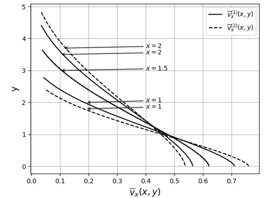
Consider first the velocity profile of ${\overline{v}}_x(x,y)$ plotted against y at a fixed x. From the analytical solutions it can be verified that

$$\begin{array}{ccc}\hfill \frac{{\overline{v}}_x^{\left(1\right)}(x,0)}{{\overline{v}}_x^{\left(2\right)}(x,0)}& ={\left(\frac{2x}{3}\right)}^{\frac{1}{6}},\hfill & \hfill \frac{y_B^{\left(1\right)}\left(x\right)}{y_B^{\left(2\right)}\left(x\right)}={\left(\frac{2}{3}x\right)}^{-\frac{1}{3}}\end{array}$$

(270)

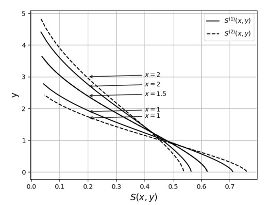
For $0<x<\frac{3}{2}$, ${\overline{v}}_x^{\left(1\right)}(x,0)<{\overline{v}}_x^{\left(2\right)}(x,0)$ and $y_B^{\left(1\right)}\left(x\right)>y_B^{\left(2\right)}\left(x\right)$ while for $x>\frac{3}{2}$ the opposite is the case. For $x=\frac{3}{2}$, the two velocity profiles coincide. This is illustrated in Figure 3 for $x=1$, $x=\frac{3}{2}$ and $x=2$. From the analytical solution it can also be verified that for the temperature difference

$$\frac{S^{\left(1\right)}(x,0)}{S^{\left(2\right)}(x,0)}={\left(\frac{2x}{3}\right)}^{\frac{1}{6}}$$

(271)

which is the same as the ratio of velocities. The temperature difference also vanishes on the boundary $y=y_B\left(x\right)$. The temperature difference for the two solutions is illustrated in Figure 4. The preferred solution for vanishing $\nu$ and $\kappa$ is the limit solution $\nu \to 0$ and $\kappa \to 0$ because it evolves continuously from the solution for $\nu \ne 0$ and $\kappa \ne 0$.

Figure 3. Graphs of ${\overline{v}}_x^{\left(1\right)}(x,y)$ for $\nu \to 0$ given by (218) and (223) and ${\overline{v}}_x^{\left(2\right)}(x,y)$ for $\nu =0$ given by (237) and (242) plotted against y for $x=1$, $x=\frac{3}{2}$ and $x=2$.

Figure 4. Graphs of $S^{\left(1\right)}(x,y)$ for $\nu \to 0$ and $\kappa \to 0$ given by (217), (220) and (224) and $S^{\left(2\right)}(x,y)$ for $\nu =0$ and $\kappa =0$ given by (236), (239) and (243) plotted against y for $x=1$, $x=\frac{3}{2}$ and $x=2$.

From the solution for $\nu \to 0$ and $\kappa \to 0$,

$${\overline{v}}_x(x,0)={\left(\frac{J}{2\rho }\mathsf{\Gamma }\left(\frac{1}{3}\right)\right)}^{\frac{1}{2}}\frac{1}{\mathsf{\Gamma }\left(\frac{2}{3}\right)}{\left(\frac{1}{\sqrt{3}{l}_{1}x}\right)}^{\frac{1}{3}},$$

(272)

$$y_B\left(x\right)=\frac{4\sqrt{3}}{9}\pi {\left(\sqrt{3}{l}_{1}x\right)}^{\frac{2}{3}}.$$

(273)

The mean velocity on the centre line increases with the strength of the jet as $J^{\frac{1}{2}}$ and decrease with the mixing length and distance as ${\left(l_{1}x\right)}^{-\frac{1}{3}}$. In comparison for the laminar jet, the velocity on the centre line increases as $J^{2/3}$ but like the turbulent jet it decreases as $x^{-\frac{1}{3}}$. The width of the turbulent jet, $y_B\left(x\right)$, is independent of J and increases with the mixing length and distance x as ${\left(l_{1}x\right)}^{2/3}$ due to turbulent diffusion. The laminar jet extends to $y=\pm \infty$. In Figure 5, the velocity profile

$$\begin{array}{cccc}\hfill {\overline{v}}_x(x,y)& =x^{-\frac{1}{3}}\frac{dF}{d\xi },\hfill & \hfill y& =\xi x^{\frac{2}{3}},\hfill \end{array}$$

(274)

is plotted at $x=1$ for $\nu =0,0.1,0.5$ and 1. For $\nu =0$ the analytical solution (218) for $\nu \to 0$, $\kappa \to 0$ is used and the numerical solution is used for $\nu >0$. We see from Figure 5 that as $\nu$ increases the mean velocity on the centre line decreases but the effective width of the jet increases due to diffusion. As $\nu$ tends to zero the numerical result tends to the analytical result. When $\frac{dF}{d\xi }$ is sufficiently small we cannot reliably determine whether $\frac{dF}{d\xi }$ is zero or non-zero since its values are within the tolerance of the numerical scheme. When the numerical scheme is used to determine the limit solution $\nu \to 0$, $\frac{dF}{d\xi }$ becomes complex for $\xi >{\xi }_B$ but when $\nu \ne 0$, $\frac{dF}{d\xi }$ remains real for all considered values of $\xi$. This suggests that $\frac{dF}{d\xi }$ remains positive for all positive values $\xi >0$, which supports the argument that $y_B\left(x\right)$ is infinite when $\nu \ne 0$ and $\kappa \ne 0$.

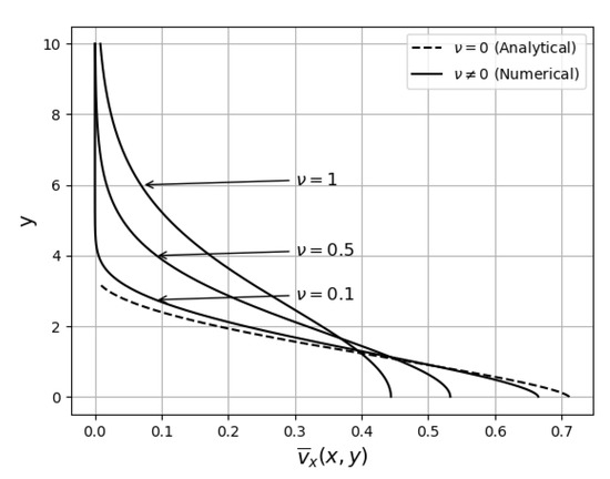
Figure 5. Velocity profiles of ${\overline{v}}_x^{\left(1\right)}(x,y)$ given by (274) plotted against y at $x=1$ for $\nu =0$, $\nu =0.1$, $\nu =0.5$ and $\nu =1$.

The effective mean shear stress is

$${\overline{\tau }}_{xy}(x,y)=\left(\mu +{\mu }_T\right)\frac{\partial {\overline{v}}_x}{\partial y}=\rho \left(\nu -l^2\left(x\right)\frac{\partial {\overline{v}}_x}{\partial y}\right)\frac{\partial {\overline{v}}_x}{\partial y}=\frac{\rho }{x}\left(\nu -l_1^2\frac{d^{2}F}{d{\xi }^2}\right)\frac{d^{2}F}{d{\xi }^2}.$$

(275)

For $\nu \to 0$ and $\kappa \to 0$

$${\overline{\tau }}_{xy}(x,y)=-\frac{\rho }{3^{4/3}{l}_1^{2/3}x}F\left(\xi \right){\left[F^{3/2}\left({\xi }_B\right)-F^{3/2}\left(\xi \right)\right]}^{2/3}.$$

(276)

In Figure 6, ${\overline{\tau }}_{xy}(x,y)$ is plotted against y for $\nu =0$, 0.1, 0.5 and 1 using (276) for $\nu =0$ and the numerical solution for $\nu >0$. As $\nu$ tends to zero the numerical result tends to the analytical result. The shear layer of the jet is the region where ${\overline{\tau }}_{xy}$ is most negative. For $\nu =0$, the width of the shear layer is $O\left({\xi }_B{x}^{2/3}\right)$. As the kinematic viscosity increases the width of the shear layer increases due to the increase in diffusion.

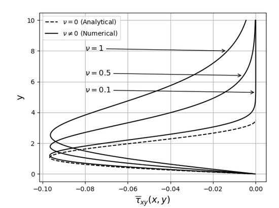
Figure 6. Effective mean shear stress ${\overline{\tau }}_{xy}=\left(\mu +{\mu }_T\right)\frac{\partial {\overline{v}}_x}{\partial y}$ plotted against y at $x=1$ for $\nu =0$, $\nu =0.1$, $\nu =0.5$ and $\nu =1$.

A property of turbulent shear flows is that they entrain fluid from the surrounding ambient fluid [23]. The process is referred to as entrainment. For $\nu =0$, ${\overline{v}}_y(x,y)$ is given by (219). On the boundary $y=y_B\left(x\right)$,

$${\overline{v}}_y(x,y_B\left(x\right))=-\frac{1}{3}{x}^{-\frac{2}{3}}F\left({\xi }_B\right)=-\frac{1}{3}{x}^{-\frac{2}{3}}{\left(\frac{J}{2\rho }\mathsf{\Gamma }\left(\frac{1}{3}\right)\right)}^{\frac{1}{2}}\frac{{\left(\sqrt{3}{l}_1\right)}^{\frac{1}{3}}}{\mathsf{\Gamma }\left(\frac{2}{3}\right)}.$$

(277)

The y-component of velocity is negative on the boundary and there is an inflow of fluid at the boundary. The entrainment increases with the strength of the jet as $J^{\frac{1}{2}}$ and decreases with distance as $x^{-\frac{2}{3}}$. In Figure 7, ${\overline{v}}_y(x,y)$ is plotted against y for $\nu =0,0.1,0.5$ and 1. For $\nu =0$ the analytical solution (219) is used while for $\nu >0$ the solution is derived numerically with ${\overline{v}}_y(x,y)$ given by (148). We see that as $\nu$ tends to zero the numerical result tends to the analytical result. There is also entrainment in a laminar two-dimensional jet which extends to $y=\pm \infty$. For a laminar jet

$${\overline{v}}_y(x,\infty )=-{\left(\frac{\nu J}{6\rho }\right)}^{\frac{1}{3}}{x}^{-\frac{2}{3}}$$

(278)

Figure 7. The y component of fluid velocity ${\overline{v}}_y$ given by (219) for $\nu =0$ and by (148) for $\nu >0$ plotted against y at $x=1$ for $\nu =0$, $\nu =0.1$, $\nu =0.5$ and $\nu =1$.

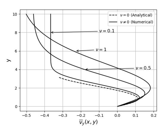
The entrainment increases more slowly with J as $J^{\frac{1}{3}}$ but decreases with the distance $x^{-2/3}$ as for a turbulent jet.

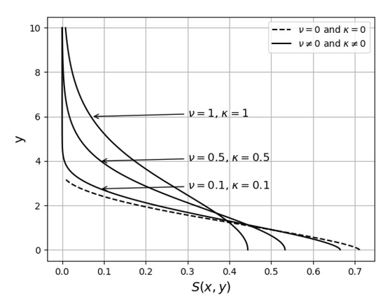
Consider next the mean temperature difference, $S(x,y)$. From the solution for $\nu \to 0$ and $\kappa \to 0$,

$$S(x,0)=\frac{3K}{4\rho c_v}{\left(\frac{2\rho }{J\mathsf{\Gamma }\left(\frac{1}{3}\right)}\right)}^{\frac{1}{2}}\left(\frac{l_2}{l_1}+1\right)\frac{\mathsf{\Gamma }\left(\frac{2}{3}\left(1+\frac{l_1}{l_2}\right)\right)}{\mathsf{\Gamma }\left(\frac{2}{3}\frac{l_1}{l_2}\right)}\frac{1}{{\left(\sqrt{3}{l}_{1}x\right)}^{\frac{1}{3}}}.$$

(279)

We see that when $\nu =0$ and $\kappa =0$ the mean temperature difference on the centre line is proportional to the total heat flux K and decreases with the total momentum flux as $J^{-\frac{1}{2}}$. It decrease with distance x and mixing length $l_1$ as ${\left(l_{1}x\right)}^{-\frac{1}{3}}$ which is the same as for the mean velocity. Otherwise it depends on the mixing lengths $l_1$ and $l_2$ through the ratio $l_1/l_2$. The width of the jet at position x is again $y_B\left(x\right)$ given by (273). The width is independent of J and K and

$$\frac{y_B\left(x\right)}{S(x,0)}\propto l_{1}x$$

(280)

as a result of turbulent diffusion of momentum and heat. In Figure 8, the profile of the mean temperature difference

$$S(x,y)=x^{-\frac{1}{3}}G\left(\xi \right)$$

(281)

is plotted at $x=1$ for $\nu =0$ and $\kappa =0$, $\nu =0.1$ and $\kappa =0.1$, $\nu =0.5$ and $\kappa =0.5$ and $\nu =1$ and $\kappa =1$. For $\nu =0$ and $\kappa =0$ the solution (220) for $\nu \to 0$ and $\kappa \to 0$ is used and the numerical solution is used for $\nu >0$ and $\kappa >0$. As $\nu$ and $\kappa$ tend zero the numerical result tends to the analytical result. We see from Figure 8 that as $\nu$ and $\kappa$ increase the temperature difference on the centre line decreases but the effective width of the jet increases due to the diffusion constants $\nu$ and $\kappa$ being non-zero. The numerical solution for $G\left(\xi \right)$ tended to zero as $\xi$ increased but never became complex for all values for $\xi$ considered. This supported the claim that the jet is unbounded in the y-direction when $\nu \ne 0$ and $\kappa \ne 0$.

Figure 8. Mean temperature difference profiles of $S(x,y)$ given by (217), (220) and (224) for $\nu =0$ and $\kappa =0$ and by (217) for $\nu >0$, $\kappa >0$ plotted against y at $x=1$ for $\nu =0\mathrm{and}\kappa =0,$$\nu =0.1\mathrm{and}\kappa =0.1,$$\nu =0.5\mathrm{and}\kappa =0.5,$$\nu =1\mathrm{and}\kappa =1$.

We now compare the streamlines of the mean flow for $\nu \to 0$, $\kappa \to 0$ and $\nu =0$, $\kappa =0$. The streamline pattern is symmetrical about the x-axis. For $\nu \to 0$, $\kappa \to 0$ the streamlines in the upper and lower half of the jet are from (227) and (228) given by

$$y=\pm x^{\frac{2}{3}}{\left(\sqrt{3}{l}_1\right)}^{\frac{2}{3}}{\int }_0^{{\left(\frac{x_0}{x}\right)}^{\frac{1}{3}}}\frac{dg}{{\left(1-g^{3/2}\right)}^{2/3}},$$

(282)

where $0<x_0<\infty$. A streamline starts at the point $(x_0,y_B\left(x_0\right))$ on the boundary of the jet where

$$y_B\left(x_0\right)={\xi }_B{x}_0^{2/3}$$

(283)

with ${\xi }_B$ given by (223) and extends to $x=+\infty$. The streamlines are plotted for a discrete range of values of $x_0$ in Figure 9.

Figure 9. Streamlines of the mean flow for the limit $\nu \to 0$ given by (282). The boundary of the jet is $y={\xi }_B{x}^{2/3}$ where ${\xi }_B$ is given by (223).

For $\nu =0$ and $\kappa =0$ the streamlines in the upper and lower half of the jet are from (244) and (245) given by

$$y=\pm x{\left(\sqrt{2}{l}_1\right)}^{\frac{2}{3}}{\int }_0^{{\left(\frac{x_0}{x}\right)}^{\frac{1}{2}}}\frac{dg}{{\left(1-g^{3/2}\right)}^{2/3}}$$

(284)

where $0<x_0<\infty$. A streamline starts at the point $(x_0,y_B\left(x_0\right))$ on the boundary of the jet where

$$y_B\left(x_0\right)={\xi }_B{x}_0$$

(285)

with ${\xi }_B$ is given by (242) and extends to $x=+\infty$. The streamlines are plotted for a discrete range of values of $x_0$ in Figure 10. The entrainment of the fluid at the boundary is clearly seen in Figure 9 and Figure 10. Since ${\overline{v}}_x(x,y_B\left(x\right))=0$ the fluid enters the jet at the boundary in the $\mp y$-direction in the upper and lower half of the jet. The main difference between the streamline pattern in Figure 9 and Figure 10 is the boundary of the jet and the dependence on x. For both solutions the parameters on which the streamlines and the boundary of the jet depend are the mixing length $l_1$, J and $\rho$.

Figure 10. Streamlines of the mean flow for $\nu =0$ given by (284). The boundary of the jet is $y={\xi }_{B}x$ where ${\xi }_B$ is given by (242).

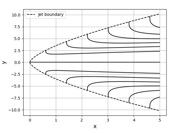
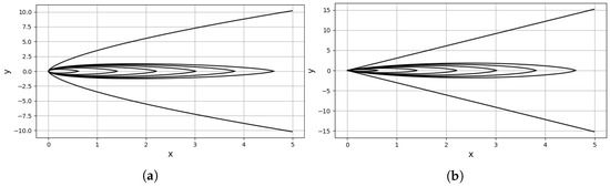
Finally we compare the lines of constant mean temperature difference for $\nu \to 0$, $\kappa \to 0$ and $\nu =0$ and $\kappa =0$. The lines of constant mean temperature difference are symmetrical about the centre line of the jet. For $\nu \to 0$, $\kappa \to 0$ a line of constant mean temperature difference in the upper and lower half of the jet is given by (233):

$$y=\pm x^{\frac{2}{3}}{\left(\sqrt{3}{l}_1\right)}^{\frac{2}{3}}{\int }_0^{{\left[1-{\left(\frac{x}{x_0}\right)}^{\frac{l_2}{2l_1}}\right]}^{\frac{2}{3}}}\frac{dg}{{\left(1-g^{\frac{3}{2}}\right)}^{\frac{2}{3}}}.$$

(286)

The point $x_0$ on the centre line is related to the temperature difference $c_0$ on the line by

$$c_0=\frac{G\left(0\right)}{x_0^{1/3}}$$

(287)

where $G\left(0\right)$ is given by (224). The lines of constant mean temperature difference are plotted in Figure 11 by giving $x_0$ a range of discrete values on the centre line. The mean temperature difference on each line is obtained from (287). Each line starts at the orifice $x=0$ and proceeds into the upper and lower half of the jet ending at a point $x_0$ with gradient negative and positive infinity. When $x_0=\infty$, (286) reduces to the equation of the boundary of the jet (273) on which the mean temperature difference $c=0$. For $\nu =0$ and $\kappa =0$ a line of constant mean temperature difference in the upper and lower half of the jet is given by (246):

$$y=\pm x{\left(\sqrt{2}{l}_1\right)}^{\frac{2}{3}}{\int }_0^{{\left[1-{\left(\frac{x}{x_0}\right)}^{\frac{3}{4}\frac{l_2}{l_1}}\right]}^{\frac{2}{3}}}\frac{dg}{{\left(1-g^{\frac{3}{2}}\right)}^{\frac{2}{3}}}.$$

(288)

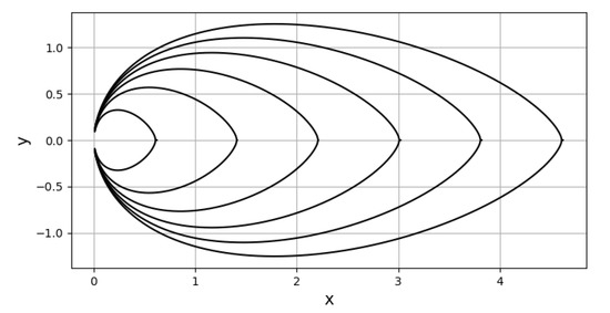
Figure 11. Lines of constant mean temperature difference for the limit $\nu \to 0$ and $\kappa \to 0$ given by (286).

The mean temperature difference $c_0$ on the line is

$$c_0=\frac{G\left(0\right)}{x_0^{1/2}}$$

(289)

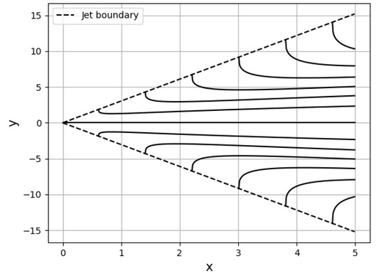
with $G\left(0\right)$ given by (243). The lines of constant mean temperature difference are plotted in Figure 12. A line starts at the orifice $x=0$ and extends into the upper and lower half of the jet. It ends at the point $x_0$ with gradient negative and positive infinity. When $x_0=\infty$ the mean temperature difference $c=0$ and (288) reduces to the boundary of the jet,

$$y_B\left(x\right)=\frac{4\sqrt{3}}{9}\pi {\left(\sqrt{2}{l}_1\right)}^{2/3}x.$$

(290)

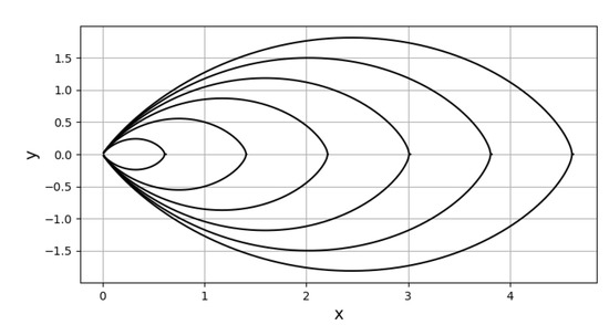
Figure 12. Lines of constant mean temperature difference for $\nu =0$ and $\kappa =0$ given by (288).

The pattern of the lines of constant mean temperature difference in Figure 11 and Figure 12 differ largely due to the different jet boundaries and different x dependence. The lines of constant mean temperature difference depend through $G\left(0\right)$ on the ratio of the mixing lengths, $l_1$ and $l_2$, K, J, $\rho$ and $c_v$.

Our preferred solution for the approximation of vanishing kinematic viscosity and thermal conductivity is the solution obtained by letting $\nu \to 0$, $\kappa \to 0$ because it evolves continuously from the numerical solution for $\nu \ne 0$, $\kappa \ne 0$ as illustrated in Figure 5, Figure 6 and Figure 7. The solution derived by Howarth [5] is the same as our solution for $\nu =0$, $\kappa =0$ with Prandl’s hypothesis because Howarth assumed that there is similarity between the fluid flow at different sections $x=\mathrm{constant}$ of the jet, that the mixing length is constant across a section ($l=l\left(x\right)$) and proportional to the breadth of a section.

We saw from the graphs in Figure 3, Figure 4 and Figure 5, Figure 7 and Figure 8 that the effect of the kinematic viscosity and thermal conductivity is to broaden the profiles due to diffusion of momentum and heat and to decrease the magnitude of ${\overline{v}}_x$, ${\overline{v}}_y$ and S on the axis of the jet due to friction between fluid elements. Entrainment of fluid at the boundary is clearly seen in Figure 7, Figure 9 and Figure 10 in which there is inflow of fluid at the boundary.

The momentum boundary and the thermal boundary of the jet coincide because the eddy kinematic viscosity ${\nu }_T$ and the eddy thermal conductivity ${\kappa }_T$ given by (36) and (37) both vanish when the mean velocity gradient $\frac{\partial {\overline{v}}_x}{\partial y}$ vanishes. If the approximation is made that $\nu =0$ and $\kappa =0$ then the thermal jet is bounded in the y-direction. However, although $\nu$ and $\kappa$ may be small compared with ${\nu }_T$ and ${\kappa }_T$ they are never zero in a real fluid and the jet will be unbounded in the y-direction. We see from Figure 5, Figure 6, Figure 7 and Figure 8 that the jet will be very weak beyond the boundary determined by the limiting solution, $\nu \to 0$, $\kappa \to 0$, which therefore determines the effective width of the wake.

The analytical solutions for $\psi (x,y)$ and $S(x,y)$ when $\nu =0$, $\kappa =0$ derived using Lie symmetry analysis could be readily adapted to give the equations of the streamlines of the mean flow and the lines of constant temperature difference. From Figure 11, Figure 12 and Figure 13 we see that the two solutions for the streamlines and lines of constant temperature difference differ mainly in the vicinity of the boundary of the thermal jet.

Figure 13. Lines of constant mean temperature difference showing the boundary of the thermal jet. (a) Limit $\nu \to 0$ and $\kappa \to 0$ given by (286) with boundary $y={\xi }_B{x}^{2/3}$ where ${\xi }_B$ is given by (223). (b) $\nu =0$ and $\kappa =0$ given by (288) with boundary $y={\xi }_{B}x$ where ${\xi }_B$ is given by (242).

8. Conclusions

The turbulent thermal jet was described by the Reynolds averaged momentum balance equation and averaged energy balance equation in the boundary layer approximation. The turbulence was described by the eddy viscosity and the eddy thermal conductivity. The eddy viscosity and eddy thermal conductivity where modelled using mixing lengths. The mixing lengths were assumed to be functions only of the distance from the orifice along the centre line of the jet.

The conserved vectors for the mean momentum flux and the mean heat flux and the conserved quantities derived from the conserved vectors played an essential role in the analysis. The associated Lie point symmetry derived using the two conserved vectors generated the invariant solution. The conserved quantity for the mean momentum flux determined the equation of the finite boundary of the jet when $\nu =0$ and $\kappa =0$. The two conserved quantities were targets in the numerical shooting method when $\nu \ne 0$ and $\kappa \ne 0$. The derivation of the associated Lie point symmetry was much easier than the derivation of the full Lie point symmetry because prolongations only to second order were required. From the double reduction theorem the two reduced ordinary differential equations could be integrated at least once because they were derived from a Lie point symmetry associated with the conserved vectors.

When $\nu =0$ and $\kappa =0$ the form of the jet is purely due to turbulent diffusion of momentum and heat. Using the associated Lie point symmetry, the mixing lengths remained arbitrary functions, but were shown to be proportional to each other. We imposed Prandtl’s hypothesis that the mixing length is proportional to the width of the jet to obtain the functional forms of the mixing lengths and hence the invariant solution. The solution derived using Prandtl’s hypothesis is different from the solution obtained by letting $\nu \to 0$ and $\kappa \to 0$. Both solutions could be solved analytically and for both the jet was bounded in the transverse y-direction. The solution $\nu \to 0$, $\kappa \to 0$ is preferred because it evolves continuously from the solution for $\nu \ne 0$ and $\kappa \ne 0$.

For $\nu \ne 0$ and $\kappa \ne 0$ the solution was derived numerically using the shooting method. The numerical solution tended to the analytical solution, $\nu \to 0$, $\kappa \to 0$, as the kinematic viscosity and thermal conductivity were decreased. The numerical solution was also used to calculate the boundary parameter ${\xi }_B$ for the uncoupled system (261), (262) and (264) when $\nu =0$ and it matched the value obtained analytically. The numerical scheme is not applicable when $\kappa =0$ since there is a singularity at $\xi =0$ in (263). As with any numerical scheme, the numerical solution could not reliably determine if the jet is unbounded in the y-direction when $\nu \ne 0$ and $\kappa \ne 0$. However, when $\nu \ne 0$ and $\kappa \ne 0$, because ${\nu }_T\to 0$ and ${\kappa }_T\to 0$ as $y\to \infty$, for sufficiently large values of y, $\nu >{\nu }_T$ and $\kappa >{\kappa }_T$ and the jet behaves like a laminar jet which extends to $y=\infty$.

The form of the invariant solutions for $\nu =0$, $\kappa =0$ and $\nu \to 0$, $\kappa \to 0$ readily leads to analytical results for the streamlines of the mean flow and the lines of constant temperature difference. The graphs in Figure 9 to Figure 13 give a comparison of the analytical solutions for vanishing kinematic viscosity and thermal conductivity and show the relation between the finite boundaries of the jets and the streamlines of the mean flow and the lines of constant mean temperature difference. The finite boundaries are lines of zero mean temperature difference.

Several novel results for the two-dimensional turbulent thermal jet have been derived. The derivation of the conservation laws and conserved vectors using the multiplier method was new. This lead to a systematic method of deriving the conserved quantities and the associated Lie point symmetry. In the numerical method, shooting to two targets which were conserved quantities was new. Prior work shot to only one conserved quantity. There are two possible solutions for vanishing kinematic viscosity and thermal conductivity, the solution $\nu \to 0$, $\kappa \to 0$ and the solution for $\nu =0$, $\kappa =0$ and our investigation of the two solutions and which is to be used was new. Howarth [5] worked with the latter solution which requires the additional assumption that the mixing length is proportional to the distance to the boundary of the jet. Our results showed that the solution does not meet smoothly with the solution for $\nu \ne 0$ and $\kappa \ne 0$. The analytical solutions for the streamlines of the mean flow and the lines of constant mean temperature difference when $\nu =0$ and $\kappa =0$ are new for the two-dimensional turbulent thermal jet. The graphs of the lines help to visualize the flow.

The most important result was to show that Lie symmetry analysis can be applied to problems like the two-dimensional turbulent thermal free jet and yield results directly and without lengthy calculations.

References

- Quinn, W.R. Turbulent free jet flows issuing from sharp-edged rectangular slots: The influence of slot aspect ratio. Exp. Therm. Fluid Sci. 1992, 5, 203–215. [Google Scholar] [CrossRef]
- Gardon, R.; Arfirat, J.C. The role of turbulence in determining heat-transfer characteristics of impinging jets. Int. J. Heat Mass Transf. 1965, 8, 1261–1272. [Google Scholar] [CrossRef]
- Tong, A.Y. On the impingement heat transfer of oblique free surface plane jet. Int. J. Heat Mass Transf. 2003, 46, 2077–2085. [Google Scholar] [CrossRef]
- Ailluad, P.; Duchaine, F.; Gicquel, L.Y.M.; Didorally, S. Secondary peak in the Nusselt number distribution of impinging jet flows: A phenomenological analysis. Phys. Fluids 2016, 28, 095110. [Google Scholar] [CrossRef]
- Howarth, L. Concerning the velocity and temperature distributions in plane and axially symmetrical jets. Proc. Camb. Phil. Soc. 1938, 34, 185. [Google Scholar] [CrossRef]
- Baron, T.; Alexander, L.G. Momentum, mass and heat transfer in jets. Chem. Engng. Prog. 1951, 47, 181–185. [Google Scholar]
- Reichardt, H. On a new theory of free turbulence. Z. Angew. Math. Mech. 1941, 21, 257–264. [Google Scholar] [CrossRef]
- Sforza, P.M.; Mons, R.F. Mass, momentum, and energy transport in turbulent free jets. Int. J. Heat Mass Transf. 1978, 21, 371–384. [Google Scholar] [CrossRef]
- Kataoka, K.; Takami, T. Experimental study of eddy diffusion model for heated turbulent thermal free jets. AIChE 1977, 23, 889–896. [Google Scholar] [CrossRef]
- Hinze, J.O.; Van der Heggezijnen, B.G. Transfer of heat and matter in the turbulent mixing zone of an axially symmetrical jet. App. Sci. Res. 1949, A1, 435–461. [Google Scholar] [CrossRef]
- Naz, R.; Mahomed, F.M.; Mason, D.P. Comparison of different approaches to conservation laws for partial differential equations in fluid mechanics. Appl. Math. Comp. 2008, 205, 212–230. [Google Scholar] [CrossRef]
- Kara, A.H.; Mahomed, F.M. Relationship between Symmetries and Conservation Laws. Inter J. Theor. Phys. 2000, 39, 23–40. [Google Scholar] [CrossRef]
- Kara, A.H.; Mahomed, F.M. A basis of conservation laws for partial differential equations. J. Nonlinear Math. Phys. 2000, 9, 60–72. [Google Scholar] [CrossRef]
- Sjoberg, A. Double reduction of PDEs from the association of symmetries with conservation laws with applications. Appl. Math. Comp. 2007, 184, 608–616. [Google Scholar] [CrossRef]
- Sjoberg, A. On double reductions from symmetries and conservation laws. Nonlinear Anal Real World Appl. 2009, 10, 3472–3477. [Google Scholar] [CrossRef]
- Mason, D.P.; Hill, D.L. Invariant solution for an axisymmetric turbulent free jet using a conserved vector. Commun. Nonlinear Sci. Numer. Simulat. 2013, 18, 1607–1622. [Google Scholar] [CrossRef]
- Magan, A.B.; Mason, D.P.; Mahomed, F.M. Analytical solution in parametric form for the two-dimensional free jet of a power-law fluid. Inter J. Non Linear Mech. 2016, 85, 94–108. [Google Scholar] [CrossRef]
- Magan, A.B.; Mason, D.P.; Mahomed, F.M. Analytical solution in parametric form for the two-dimensional liquid jet of a power-law fluid. Inter J. Non Linear Mech. 2017, 93, 53–64. [Google Scholar] [CrossRef]
- Hutchinson, A.J. Application of a modified Prandtl mixing length model to the turbulent far wake with a variable mainstream flow. Phys. Fluids 2018, 30, 95–102. [Google Scholar] [CrossRef]
- Swain, L.M. On the turbulent wake behind a body of revolution. Proc. Roy. Soc. Lond. Ser. A 1929, 125, 647–659. [Google Scholar]
- Burden, R.L.; Faires, J.D. Numerical Analysis, 9th ed.; Brookscole: Boston, MA, USA, 2011; pp. 672–684. [Google Scholar]
- Edun, I.F.; Akinlabi, G.O. Application of the shooting method for the solution of second order boundary value problems. J. Phys. Conf. Ser. 2021, 1734, 012020. [Google Scholar] [CrossRef]
- Pope, S.B. Turbulent Flows; Cambridge University Press: Cambridge, UK, 2000; pp. 92–95, 170–171. [Google Scholar]
- Schlichting, H.; Gersten, K. Boundary Layer Theory; Springer: Berlin/Heidelberg, Germany, 2000; pp. 209–211, 498, 539, 567. [Google Scholar]
- Acheson, D.J. Elementary Fluid Mechanics; Clarendon Press: Oxford, UK, 1990; Chapter 8. [Google Scholar]
- Gillepse, R.P. Integration; Oliver and Boyd: Edinburgh, Scotland, 1967; pp. 90–95. [Google Scholar]
Publisher’s Note: MDPI stays neutral with regard to jurisdictional claims in published maps and institutional affiliations. |
© 2022 by the authors. Licensee MDPI, Basel, Switzerland. This article is an open access article distributed under the terms and conditions of the Creative Commons Attribution (CC BY) license (https://creativecommons.org/licenses/by/4.0/).