Article

Symplectic Dynamics and Simultaneous Resonance Analysis of Memristor Circuit Based on Its van der Pol Oscillator

1
Shaanxi International Joint Research Center for Applied Technology of Controllable Neutron Source, School of Computer Science, Xijing University, Xi’an 710123, China
2
Xi’an Key Laboratory of Advanced Photo-Electronics Materials and Energy Conversion Device, School of Computer Science, Xijing University, Xi’an 710123, China
*
Author to whom correspondence should be addressed.
Symmetry 2022, 14(6), 1251; https://doi.org/10.3390/sym14061251
Submission received: 24 April 2022 / Revised: 9 June 2022 / Accepted: 12 June 2022 / Published: 16 June 2022
(This article belongs to the Special Issue Discrete and Continuous Memristive Nonlinear Systems and Symmetry)

Abstract

:
A non-autonomous memristor circuit based on van der Pol oscillator with double periodically forcing term is presented and discussed. Firstly, the differences of the van der Pol oscillation of memristor model between Euler method and symplectic Euler method, four-order Runge–Kutta method (RK4) and four-order symplectic Runge–Kutta–Nyström method (SRKN4), symplectic Euler method and RK4 method, and symplectic Euler method and SRKN4 method in preserving structure are compared from theoretical and numerical simulations, the symmetry and structure preserving and numerical stability of symplectic scheme are demonstrated. Moreover, the analytic solution of the primary and subharmonic simultaneous resonance of this system is obtained by using the multi-scale method. Finally, based on the resonance relation of the system, the chaotic dynamics behaviors with different parameters are studied.

1. Introduction

In 1927, the illustrious van der Pol equation was proposed to describe the oscillation effect of triodes in electronic circuits [1]. Then, in physics [2,3,4], biology [5,6] and economics [7], the van der Pol equation has become a fundamental model to describe the oscillation process. Meanwhile, the memristor was defined in 1971 as the fourth basic circuit device by Academician Chua, following the three basic Double-terminal circuit elements of resistors, capacitors and inductors [8], it can be regarded as a time-varying resistor, and its resistance depends on the amount of charge passing through it. As a fundamental passive circuit element, memristor will be widely used in circuit design as a general RLC element [9,10,11]. It is well-known that Chua’s circuit can be realized by only three elements: inductors, capacitors, and voltage-controlled memristors [12], and van der Pol equation can be realized by two elements: inductors and memristor [13]. Additionally, the time-varying characteristics of memristor give it rich dynamical behaviors [14], and a series of chaotic oscillators are established by using memristors as nonlinear components [15,16]. However, most memristor chaotic circuits developed in recent years are autonomous systems [17,18,19,20], there are few non-autonomous systems with periodically forcing terms, which introduce chaos through forcing terms and other parameters, increase regulations and are easier to be applied in practice. Therefore, it is fascinating to study the non-autonomous memristor circuit based on a van der Pol oscillator with a periodically forcing term.
All along, the numerical method has been using difference approximation to approximate calculus, but its disadvantage is that it focuses only on the extent to which the numerical solution approximates the exact solution, without giving more consideration to the geometric properties of the mechanical system itself as described by the mathematical model. Therefore, a new direction in numerical analysis is that geometric numerical integration is paid more and more attention [21,22]. The well known unpublished report by De Vogelaere is the first demonstration of the existence of numerical integrators (now called symplectic integrators) [23], and it was not until later that Feng proposed a new method to numerically integrate the Hamiltonian system based on symplectic geometry [24], and this implicit method was later applied by Channell [25]. Meanwhile, Sanz-Sema [26] and Lasagni [27] found a condition for implicit Runge–Kutta methods to be symplectic, and Ruth developed an idea of explicit symplectic schemes for the Hamiltonian of the form H = T ( p ) + V ( q ) [28]. Along the line of explicit symplectic schemes, higher order integrators were presented by Yoshida later on [29]. Then, Qin proposed a multi-step symplectic method and applied it to the numerical analysis of wave problems [30], Forest and Ruth constructed the symplectic maps for nonlinear motion of particles in accelerators [31], Yoshida modified non-existence of first integral by symplectic integration methods [32], Cieśliński compares several discretizations of the simple pendulum equation in a series of numerical experiments and puts forward a new numerical scheme of improved discrete gradient method [33]. Subsequently, the development, analysis and use of various numerical solution algorithms for differential equations concerned in geometric numerical integration [34,35,36,37,38,39]. These algorithms preserve the geometric or qualitative properties of the exact solutions, such as an integral or symmetry, or preservation of a differential invariant such as symplecticity or phase space volume. In engineering, especially for practical systems such as van der Pol and Duffing oscillator, classic numerical method are used commonly, but it has dissipation mechanisms, and errors will accumulate. Therefore, it is very urgent to study the structure preserving methods for these systems.
The path to chaos is also one of the fundamental problems in the study of dynamic behaviors of specific systems [40,41,42,43,44]. However, most of its studies are inclined towards Duffing oscillators, and the studies on periodic oscillation solutions of these systems can be divided into two categories. One is to establish a dynamic model more in line with engineering practice by considering the complexity of structure from the perspective of system structure [45]. The other is to study the dynamical behaviors of the system under complex excitation and the path leading to chaos [46,47]. Nonlinear systems are prone to resonance. In addition to the primary resonance [48], there also have some special resonance phenomena, such as super-harmonic resonance [49], sub-harmonic resonance [50], etc. However, most studies are still limited to the response law of nonlinear system under single harmonic excitation. In practical engineering, combination resonance [51] or simultaneous resonance [52,53] often occurs under multi-frequency excitation, but they are mentioned rarely, especially for van der Pol equation. The paper is organized as follows: a non-autonomous memristor circuit based on van der Pol oscillator with a double periodically forcing term is introduced, and the zero intersection and frequency-dependence characteristics of the memristor are verified by Multisim in Section 2. In Section 3, the stability and dynamic characteristics are studied, and the differences between Euler method and symplectic Euler method, four-order Runge–Kutta method and four-order Symplectic Runge–Kutta–Nyström method, symplectic Euler method and four-order Runge–Kutta method in preserving symmetry and structure are compared from theoretical and numerical simulation. In Section 4, the analytic solution of the primary and subharmonic (1/3 order) simultaneous resonance of this system is obtained by using the multi-scale method, then the chaotic dynamical behaviors are studied from the resonance relationship. Finally, concluding remarks are given in Section 5.

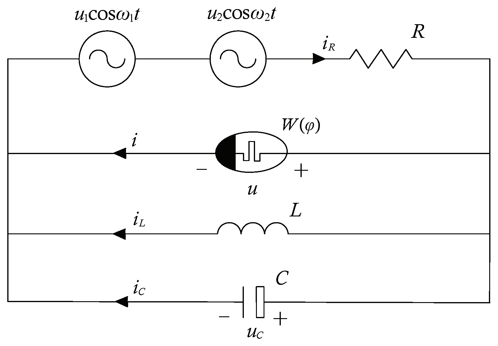
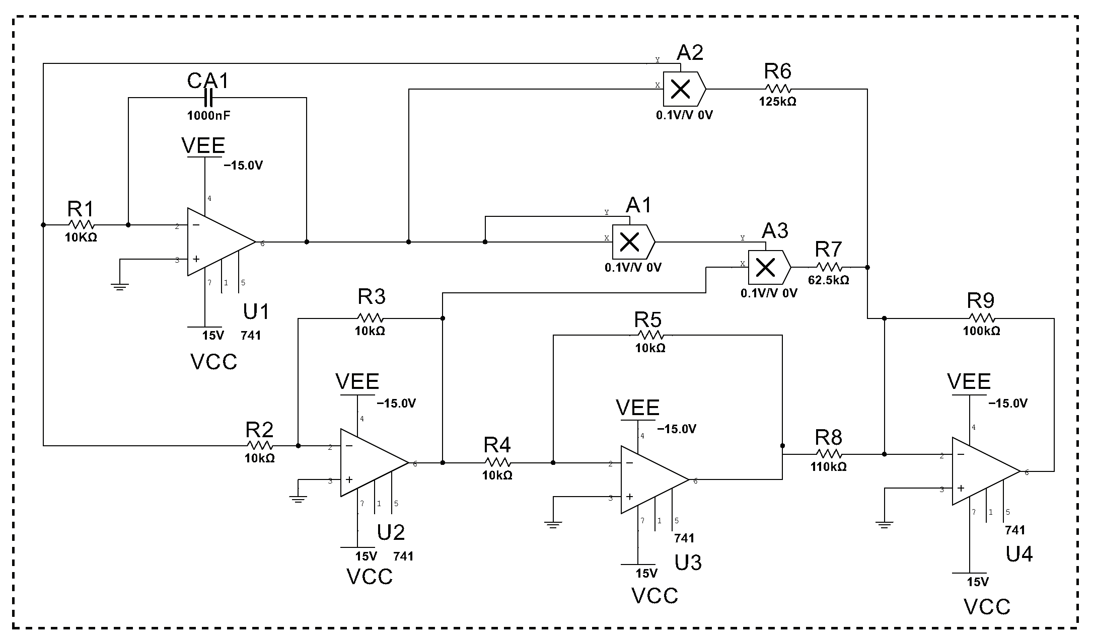
2. Memristor Circuit Based on van der Pol Oscillation Model

The memristor is a device used to describe the relationship between the magnetic flux φ and the charge q in electronic circuits, and it can be expressed by f ( φ , q ) = 0 . Memristors include charge-controlled memristor and flux-controlled memristor [54]. If the f ( φ , q ) is expressed as the single-valued function of charge, the charge-controlled memristor model is M ( q ) = d φ ( q ) d q , and it is expressed as the single-valued function of voltage, the voltage-controlled memristor model is W ( φ ) = d q ( φ ) d φ , similarly. Where, R ( q ) and W ( q ) represent the memristance and memductance of the memristor, respectively, and they are nonlinear functions that satisfy M ( q ) = 1 W ( φ ) , similar to the resistance and conductance of the resistor.
Van der Pol first derived the van der Pol equation in order to describe the oscillating effect of triodes in electronic circuits. The van der Pol system is a kind of classical self-excited oscillation system. As an important mathematical model, the van der Pol system can be widely used in complex dynamic system modeling. It provides solutions for many practical engineering problems, and its standard mathematical form is as follows:
x ˙ = y y ˙ = x + μ ( 1 x 2 ) y + A cos ω t
where, μ is nonlinear parameter, A is amplitude of applied excitation and ω is frequency of applied excitation. On the basis of the form of the system (1), Lu designed the second-order nonautonomous van der Pol oscillator in the Chua’s diode [55]. So, based on that, we add excitation source, and built a van der Pol oscillator based on this cubic memristor, as is shown in Figure 1.
The capacitor voltage u c and the magnetic flux φ of the memristor are selected as state variables, and the equation of state of the circuit can be written as
φ ˙ = u c u ˙ c = u 1 cos ω 1 t u 2 cos ω 2 t u c R C W φ u c C φ L C
where, W ( φ ) is the memductance, and its form is W ( φ ) = α φ 2 + β φ + γ , which implies q ( φ ) = α 3 φ 3 + β 2 φ 2 + γ φ . Additionally, to explore the circuit properties of the memristor, a corresponding emulator is designed, as shown inside the frame in Figure 2.
The voltage between the capacitor electrodes is defined as the internal state of the memristor, and the applied voltage and output current are set as v i and i, respectively. U 1 is inverting amplifier; A 1 , A 2 , A 3 are multipliers; U 2 , U 3 , U 4 are inverse integrators and R 1 , R 2 , R 3 , R 4 , R 5 , R 6 , R 7 , R 8 , R 9 are resistors of the memristor, the simulation results of the hysteresis curves and time series are observed, as shown in Figure 3.
As can be seen from Figure 3a, the zero intersection and frequency-dependence characteristics of the memristor are verified by Multisim, and there is an asymmetric pinched hysteresis loop with frequency f = 30 Hz and amplitude voltage v i = 5 V, which verifies the existence of non-ideal memrisitve behavior of the memristor.
Then, let x = φ , y = u c , we have
x ˙ = y y ˙ = 1 γ R R C 1 α R 1 γ R x 2 β R 1 γ R x y 1 L C x + u 1 R C cos ω 1 t + u 2 R C cos ω 2 t
The Equation (3) can be rewritten as a second-order nonautonomous differential equation:
x ¨ ξ ( 1 Δ 1 x 2 Δ 2 x ) x ˙ + ω 0 2 x = A 1 cos ω 1 t + A 2 cos ω 2 t
where, ξ = 1 γ R R C , Δ 1 = α R 1 γ R , Δ 2 = β R 1 γ R , A 1 = u 1 R C , A 2 = u 2 R C , ω 0 2 = 1 L C , here ξ denotes stiffness parameter and ξ > 0 , ω 0 is the natural frequency of this model. Additionally, the circuit model has the form of a van der Pol equation from Figure 1.

3. Symplectic Dynamic Analysis of van der Pol Self-Excited Oscillator

3.1. Equilibria and Stability

Considering remove the external excitation, the Equation (4) can be expressed as
x ¨ ξ ( 1 Δ 1 x 2 Δ 2 x ) x ˙ + ω 0 2 x = 0
and Equation (5) can be rewritten as
x ˙ = y y ˙ = ξ ( 1 Δ 1 x 2 Δ 2 x ) y ω 0 2 x
Hence, the equilibrium of the system is O ( 0 , 0 ) , and the Jacobian matrix at this equilibrium is
J = 0 1 ω 0 2 ξ
and the corresponding eigenvalue equation can be written as λ 2 ε λ + ω 0 2 = 0 , Then, it is easy to obtain the eigenvalues as
λ 1 , 2 = 1 2 ξ ± 1 2 ξ 2 ( 2 ω 0 ) 2
Lemma 1
(Lyapunov’s theorem of stability [56]). If X = f ( t , x ) , f ( t , x ) = f ( t + T , x ) , f ( t , x ) and f x are continuous. x R n has a periodic solution X * ( t ) . If the eigenvalue of the linear variational equation Y = f x ( t , X * ( t ) ) Y has strictly negative real parts, then X * ( t ) is uniformly asymptotically stable. If there is an eigenvalue with strictly positive real parts, then X * ( t ) is unstable.
Lemma 2
(Poincaré-Andronov-Hopf bifurcation existence theorem [57]). Assumption X = A ( λ ) + F ( λ , x ) is a C k , where k 3 , and the planar vector field depends on the scalar parameter λ, makes F ( λ , 0 ) = 0 , D x F ( λ , 0 ) = 0 , where λ is small sufficiently, if the equation of the linear part of A ( λ ) has a pair of pure imaginary root α ( λ ) + i β ( λ ) at the O ( 0 , 0 ) , and eigenvalue with nonzero velocity across the imaginary axis, namely d α ( 0 ) d λ 0 . Then, there is λ ¯ < λ 0 , for any U R 2 , O ( 0 , 0 ) U , for any λ 0 > 0 , λ 0 is relatively fixed, subject to the equation X has a nontrivial periodic orbits in U.
According to Lemma 1, the relationship between equilibrium state and ξ can be obtained as shown in the Table 1.
From Table 1, when ξ > 0 , equilibria are unstable, and the phase trajectory is asymptotic to the equilibrium, the movement of phase points along the phase trace deviates from the equilibrium to generate an isolated limit cycle. Meanwhile, when ξ changes from positive to negative, the equilibrium loses stability, because d Re λ 1 , 2 d ξ = 1 2 0 . According to Lemma 2, Hopf bifurcation is generated at ξ = 0 , and bifurcation produces a family of periodic solutions near the equilibrium O ( 0 , 0 ) .

3.2. Hamiltonian and Exact Solution of Oscillator

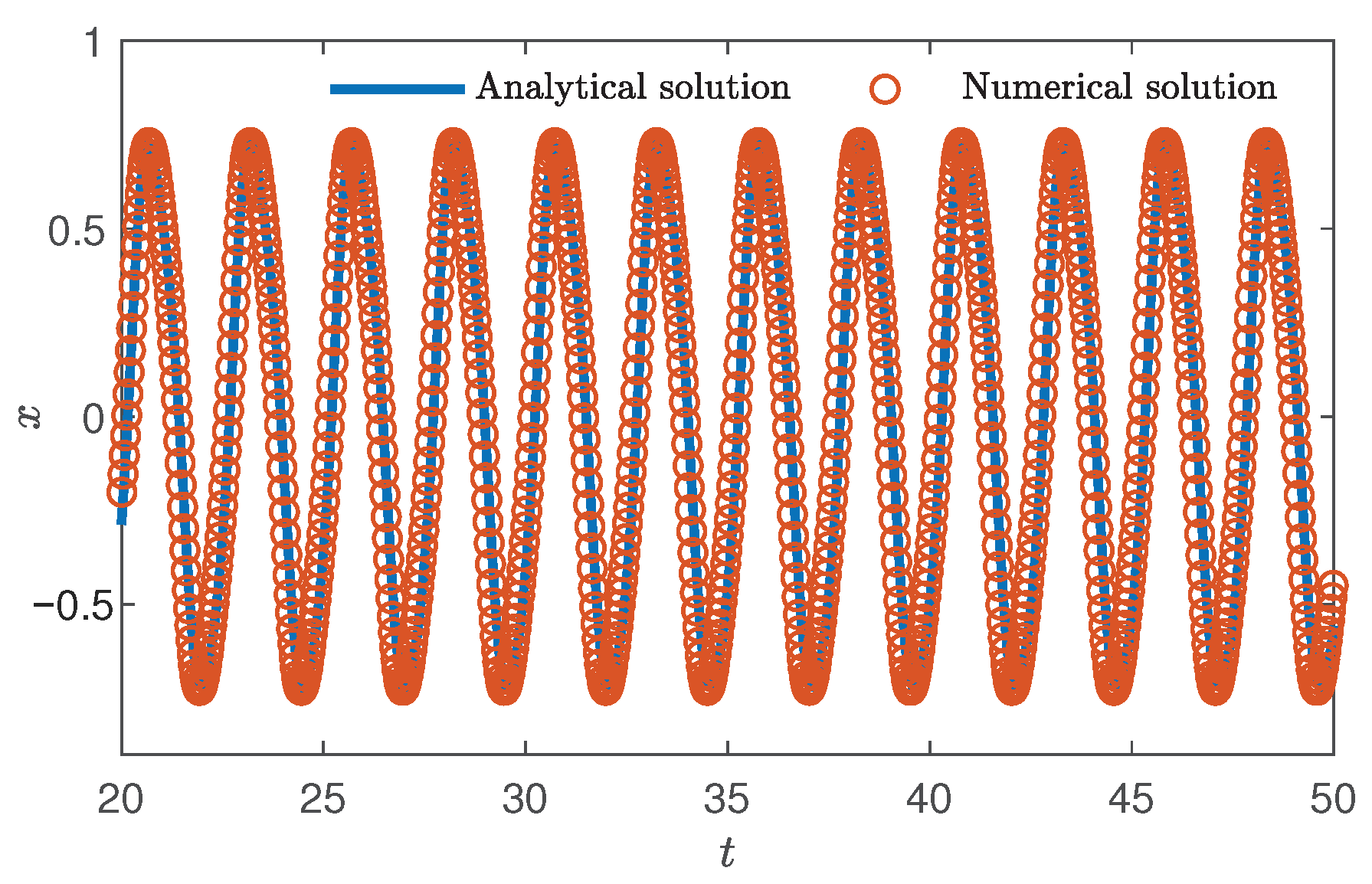
3.2.1. Exact Solution Method

Consider ξ is a disturbance term, In order to study the exactness of the solution, here let ξ = 0 , and the system (6) becomes
x ˙ = y y ˙ = ω 0 2 x
Obviously, the system (8) is the Hamilton canonical equation, and the corresponding Hamiltonian can be defined as
H ( x , y ) = ω 0 2 x 2 + y 2 2
According to Table 1, when ξ = 0 , its phase trajectory is a closed-loop orbit centered at O ( 0 , 0 ) . Here, we take the starting point ( 0 , Y 0 ) on y-axis, then, the undisturbed parameter equation with time [58] is
x ( t ) = Y 0 sin ω 0 t y ( t ) = ω 0 Y 0 cos ω 0 t
For Equation (10), when t = 0 , we have x ( t ) = 0 , y ( 0 ) = ω 0 Y 0 . Additionally, the starting point of the exact solution (symplectic scheme) is ( 0 , ω 0 Y 0 ) , the Hamiltonian becomes H ( x , y ) = ω 0 2 Y 0 2 2 . When ξ 0 , the system (6) can be written in the form of a Hamiltonian with periodic perturbation:
x ˙ = ξ f 1 ( x , y ) + H ( x , y ) y y ˙ = ξ f 2 ( x , y ) H ( x , y ) x
where, f 1 ( x , y ) = 0 and f 2 ( x , y ) = y ( 1 Δ 1 x 2 Δ 2 x ) .
Then, by the Melnikov method, we have Melnikov function
M ( Y 0 ) = 0 T ( Y 0 ) ( H ( x , y ) x f 1 ( x , y ) + H ( x , y ) y f 2 ( x , y ) ) = 0 2 π ω 0 y 2 ( 1 Δ 1 x 2 Δ 2 x ) d t
substitute Equation (10) into the Equation (12) to obtain
M ( Y 0 ) = 0 2 π ω 0 ( ω 0 Y 0 cos ω 0 t ) 2 ( 1 Δ 1 ( Y 0 sin ω 0 t ) 2 Δ 2 Y 0 sin ω 0 t ) d t = 0 2 π ω 0 ( ω 0 Y 0 cos ω 0 t ) 2 ( 1 Δ 1 ( Y 0 sin ω 0 t ) 2 ) d t 0 2 π ω 0 ( ω 0 Y 0 cos ω 0 t ) 2 ( Δ 2 Y 0 sin ω 0 t ) d t = π ω 0 Y 0 2 ( 1 1 4 Δ 1 Y 0 2 ) 0 = π ω 0 Y 0 2 ( 1 1 4 Δ 1 Y 0 2 )
When ξ 0 and smaller, the Poincaré mapping will have a hyperbolic fixed point, and the homoclinic orbital of the Hamilton system (11) will break, so as to generate stable invariant manifold W 1 and unstable invariant manifold W 2 of this fixed point. Melnikovs’ theory explains that whether W 1 and W 2 intersect determines the existence of chaos in the system. Hence, when M ( Y 0 ) = 0 , that is Y 0 = 0 or Y 0 = 2 Δ 1 , there is a sufficiently small ξ , so that stable manifolds W 1 and unstable manifolds W 2 intersect. Further, d M ( Y 0 ) d t = 4 π ω 0 δ 1 < 0 0 , there must be a transversal homoclinic point on the Poincaré section.

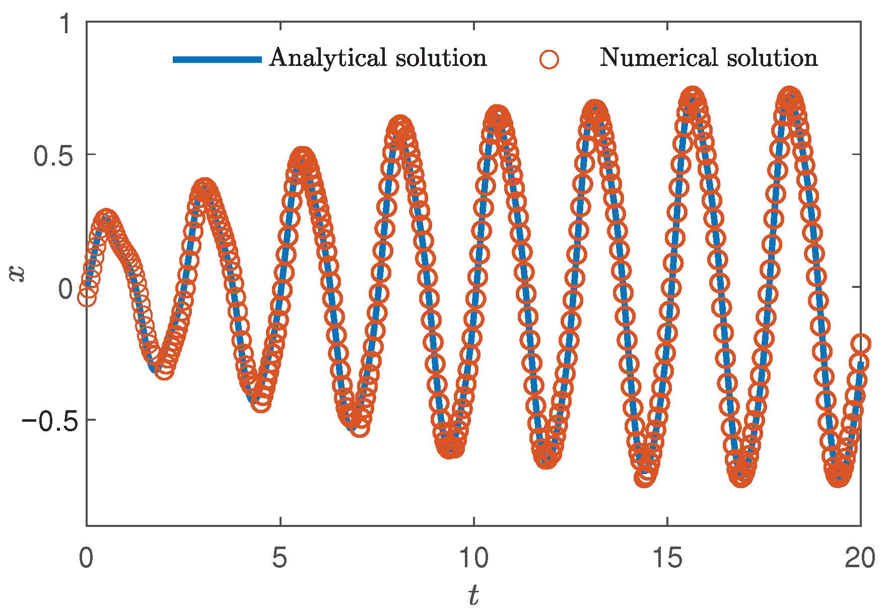
3.2.2. Numerical Simulation

For the above, assume that ξ is extremely close to 0, that is ξ = 0 , given Δ 1 = 16 , ω 0 = 10 , and obtain Y 0 = 2 Δ 1 = 0.5 , for the Equation (10), the starting point of the exact solution is ( 0 , ω 0 Y 0 ) = ( 0 , 5 ) , then the Hamiltonian is H ( x , y ) = 12.5 , and the phase diagram and time series under exact solution are shown in Figure 4.
Figure 4 shows the self-excited oscillation output under the initial condition ( 0 , 5 ) of the exact solution. The response is sinusoidal waveform with a frequency approaching ω 0 . By solving the exact solution, the comparison between symplectic and non-symplectic methods are prepared.

3.3. Solutions of Numerical Scheme

3.3.1. Euler Scheme

There are many numerical solutions for differential equations, one of these is discretization. Firstly, the approximate value y 0 , y 1 , y n 1 , y n , y n + 1 , of y ( t ) on discrete node is obtained. Then, the recurrence formula of the approximate value y n of y ( t n ) is established to obtain the approximate value of y ( t ) at each node. The spacing between two adjacent nodes is called step h = t n + 1 t n , assuming that h is constant, then node t n = t 0 + n h , n = 0 , 1 , 2 , , n . Then, defined by the derivative, Euler discretization of the equation, have
y ( t n + 1 ) y ( t n ) h = d y ( t n ) d t = f ( t n , y ( t n ) )
Through it, we can re describe as
y n + 1 = y n + h f ( t n , y n )
According to a memristor circuit based on its van der Pol oscillator without external excitation, the Equation (6) is discretized and obtained
x n + 1 = x n + h f 1 ( t n , x n , y n ) y n + 1 = y n + h f 2 ( t n , x n , y n )
where, f 1 ( t , x , y ) = x ˙ = d x d t , f 2 ( t , x , y ) = y ˙ = d y d t . Hence, the iteration format is
x n + 1 = x n + h y n y n + 1 = y n + h ξ ( 1 Δ 1 x n 2 Δ 2 x n ) y n ω 0 2 x n

3.3.2. Symplectic Euler Scheme

The algebraic relation obtained by Euler method does not depend on initial and boundary conditions. However, no matter how small the step size is, the vibration will be unbounded, and with the evolution of time, the vibration amplitude will tend to infinity, destroying the periodicity of the system. Therefore, the symplectic Euler scheme is constructed to improve the structure-preserving performance of the traditional Euler scheme, and the symplectic Euler discrete scheme is
y n + 1 = y n + h f ( t n + 1 , y n )
According to memristor circuit based on its van der Pol oscillator without external excitation, the Equation (6) is discretized and obtained
x n + 1 = x n + h f 1 ( t n , x n + 1 , y n ) y n + 1 = y n + h f 2 ( t n , x n + 1 , y n )
Hence, the iteration format of memristor circuit based on its van der Pol oscillator without external excitation is
x n + 1 = x n + h y n y n + 1 = y n + h ξ ( 1 Δ 1 x n + 1 2 Δ 2 x n + 1 ) y n ω 0 2 x n + 1
It is easy to obtain that the Jacobian matrix of Equation (20) is symplectic.

3.3.3. Four-Order Runge–Kutta Scheme

The four-order Runge–Kutta method is more widely used than Euler method in practical applications, Runge–Kutta method is a favorable tool for numerical solution of ordinary differential nonlinear equations, with high calculation accuracy. By shortening the step distance and increasing the order, the error range can be further controlled, and better results can be obtained in the case of calculation convergence. The classical method is as follows:
y n + 1 = y n + h 6 ( K 1 + 2 K 2 + 2 K 3 + K 4 ) K 1 = f ( x n , y n ) K 2 = f ( x n + h 2 , y n + h 2 K 1 ) K 3 = f ( x n + h 2 , y n + h 2 K 2 ) K 4 = f ( x n + h , y n + h K 3 )
where, h is step, and let y n = y ( t n ) , then the expression of y n + 1 is exactly identical to the first four terms of Taylor expansion of y x n + 1 at x n + 1 , and the local truncation error is O h 4 .

3.3.4. Four-Order Symplectic Runge–Kutta–Nyström Scheme

For the solution of system (8), there is the following four-order symplectic Runge–Kutta–Nyström scheme as
g i = x n + c i h y n + h 2 j = 1 s a i j f g j , i ( 1 , s ) x n + 1 = x n + h y n + h 2 j = 1 s d j f g j y n + 1 = y n + h j = 1 s b j f g j
where, b j = d j 1 c j , 1 j s and d i d j c j c i = d j a j i , 1 i < j s , and this scheme is symplectic.
The coefficient of Equation (22) are
A = a 11 a 12 a 21 a 22 a 13 a 14 a 23 a 24 a 31 a 32 a 41 a 42 a 33 a 34 a 43 a 44 = 0 0 0 0 5 12 α 2 0 0 0 0 1 2 + α 0 0 0 1 2 + α 0 0 , B = b 1 b 2 b 3 b 4 = 3 4 α 1 2 1 4 + α b 4 b 4 , C = c 1 c 2 c 3 c 4 = α 1 α α α , D = d 1 d 2 d 3 d 4 = 7 9 α 12 α 2 ( 1 α ) ( α 1 4 b 4 ) ( 1 α ) b 4 .
where, b 4 is arbitrary parameter and 6 α 2 6 α + 1 = 0 .

3.4. Numerical Simulation

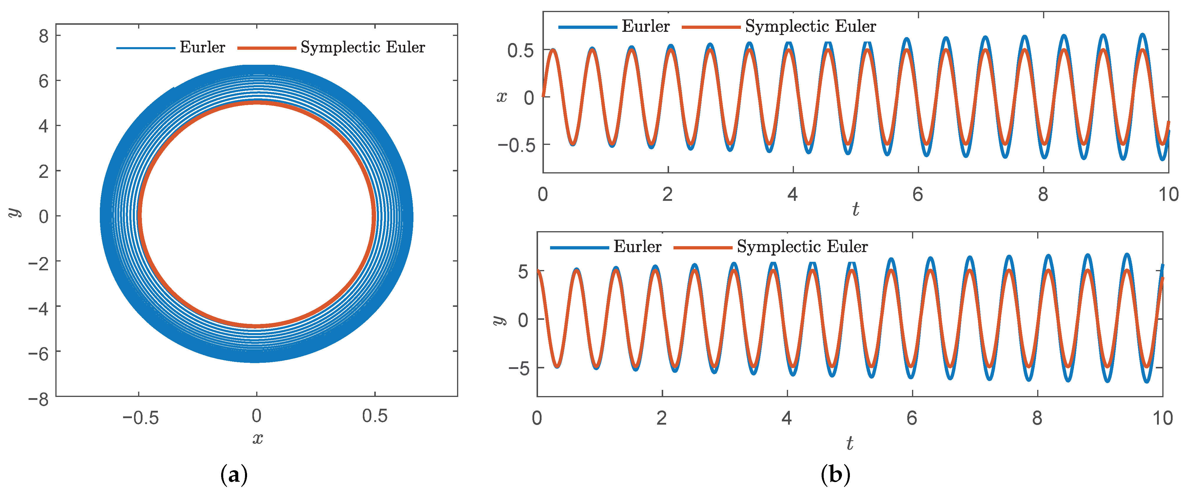
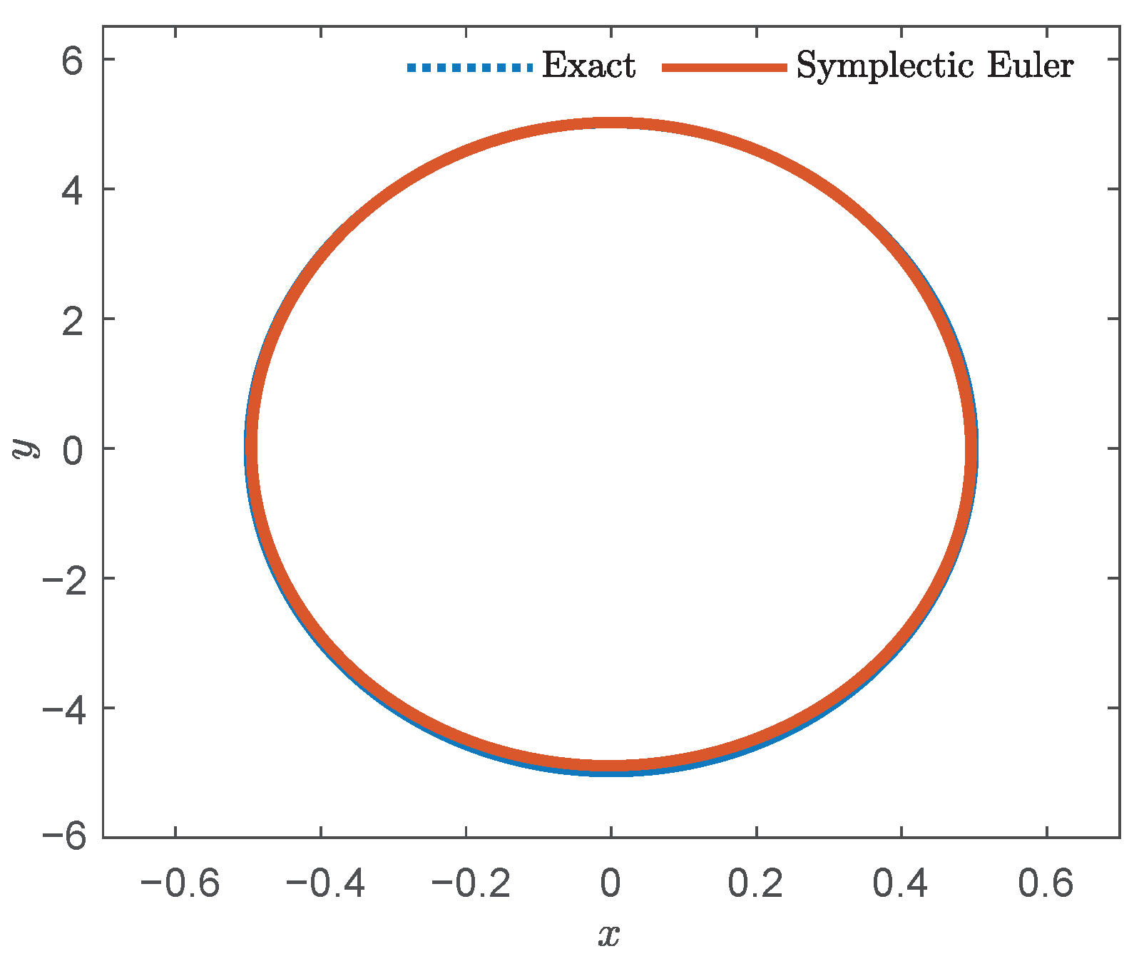
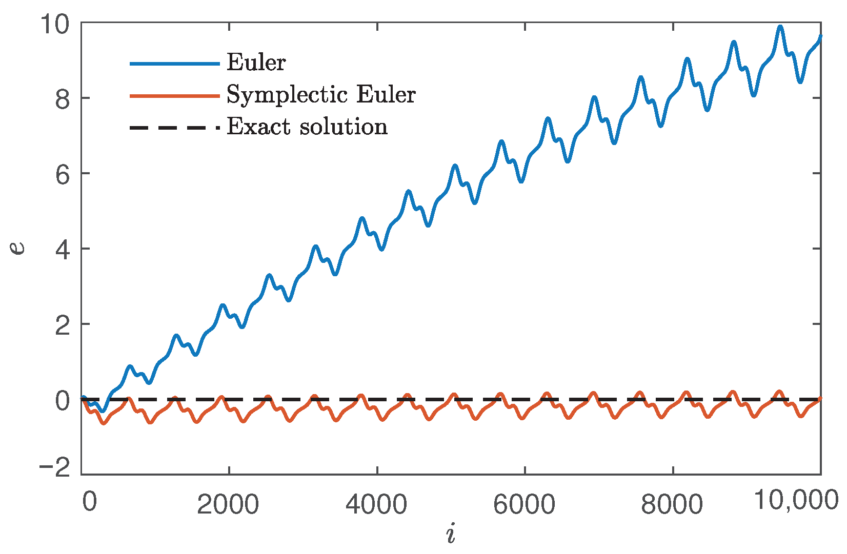
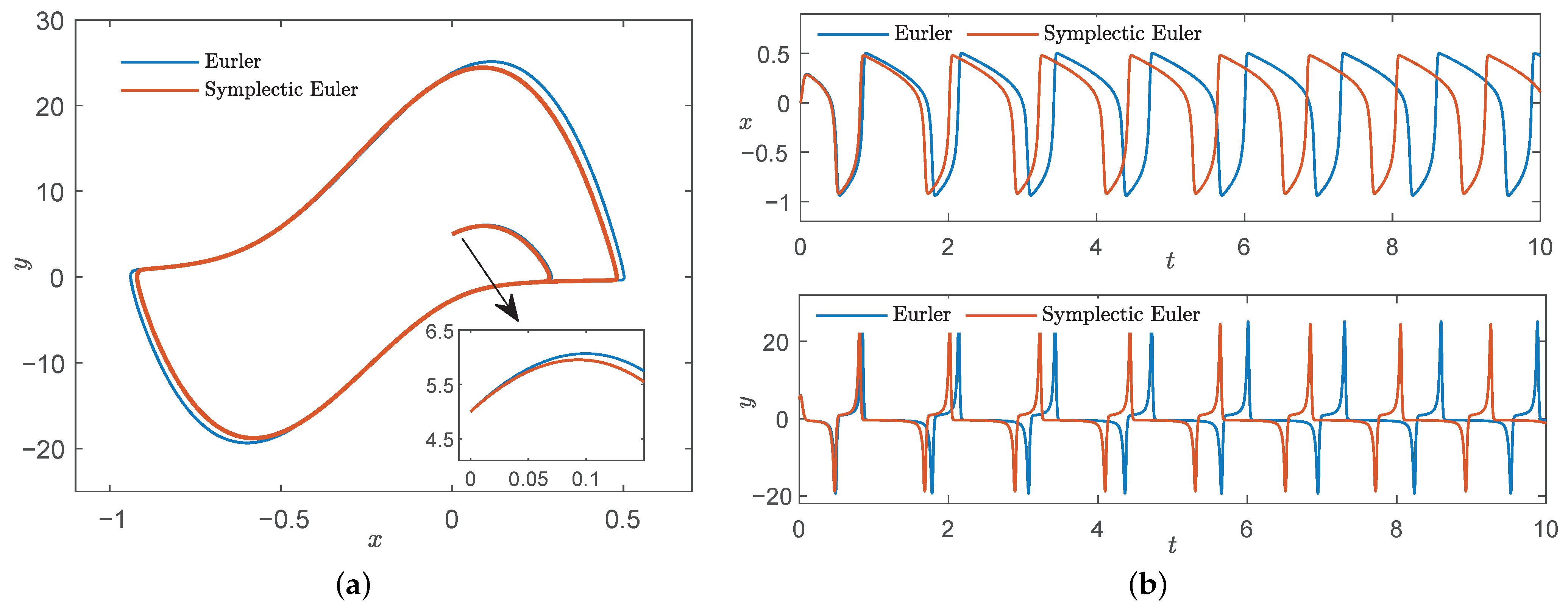
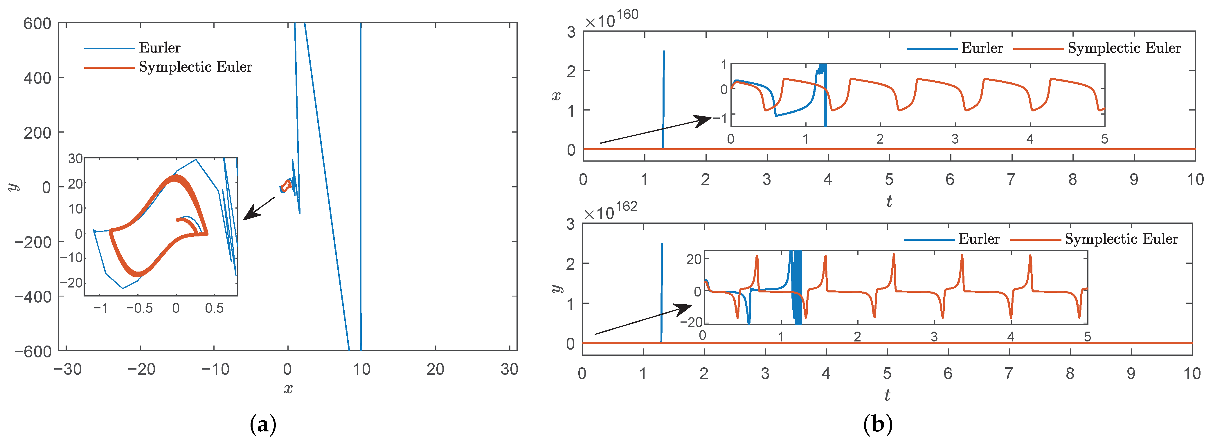
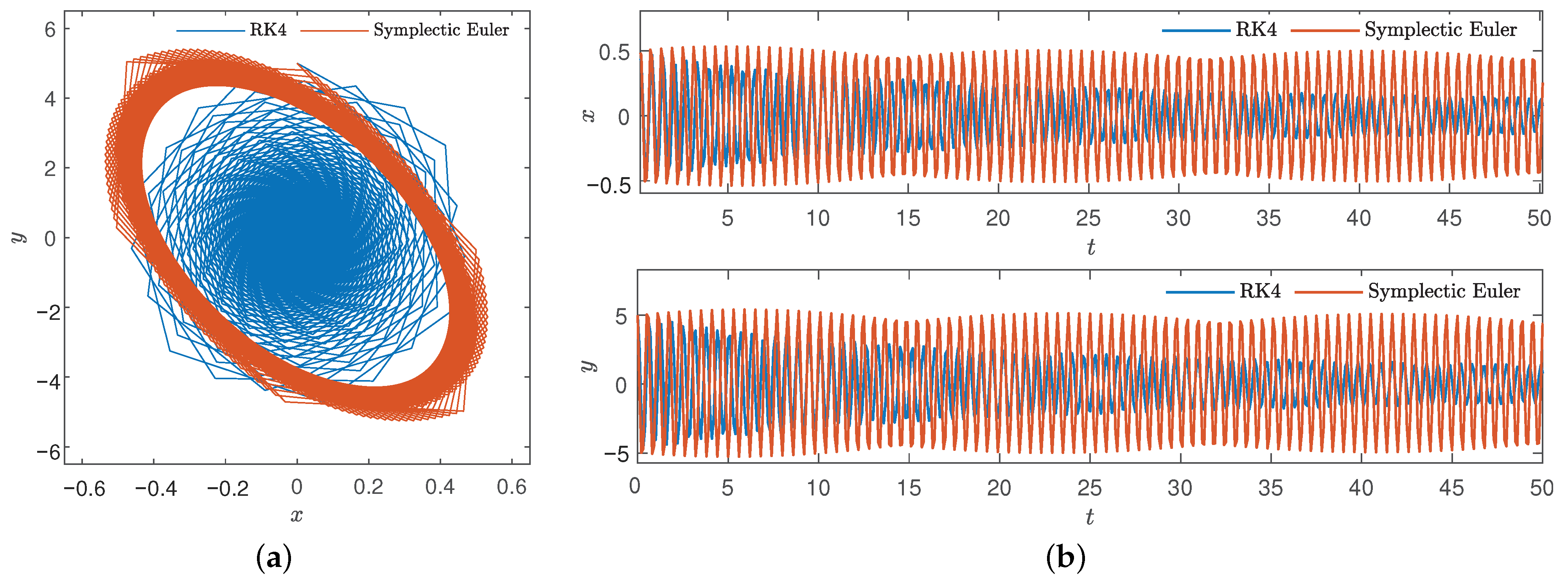
3.4.1. Euler Method and Symplectic Euler Method

a. ξ = 0.1
Here, according to Section 3.2.2, also set the starting point to ( 0 , 5 ) , given ξ = 0.1 , Δ 1 = 16 , Δ 2 = 8 , ω 0 = 10 , and set the step h = 0.001 , the number of iterations is n = 10,000. Then, the comparison of Euler and symplectic Euler phase trajectories and displacement component changes of time series were obtained in Figure 5.
From Figure 5, it can be found that the non-symplectic method leads to divergence of phase trajectory and time displacement components, it does not preserve the structure, while the symplectic method has a good effect of symmetry and structure preserving. Additionally, the comparison diagram of the exact solution and symplectic Euler method as shown in Figure 6.
Through the comparison, the symplectic method is shown to have a higher coincidence with the exact solution and the structure is preserved.
According to Section 3.2.2, we know when ξ = 0 , the Hamiltonian of the system (6) is H ( x , y ) = 12.5 . Then, we calculate the Hamiltonian under the symplectic method and the non-symplectic method when ξ is small enough, as shown in Table 2.
Therefore, a comparison diagram of error trends of different methods is presented, as shown in Figure 7.
When ξ is sufficiently small, the Hamiltonian of the system (6) remains around H ( x , y ) = 12.5 by symplectic Euler method, however, the classic Euler method diverges and does not preserve the symmetry and structure.
b. ξ = 20
In order to further illustrate the superiority of the symplectic method, we set ξ = 20 and adjust the step h based on this, which is described in two cases.
Case 1: h = 0.001 .
When the value of ξ is very large, given ξ = 20 , likewise Δ 1 = 16 , Δ 2 = 8 , ω 0 = 10 , the number of iterations n = 10,000, set the step h = 0.001 , Figure 8 shows the phase plane and time traces between the Euler method and the symplectic Euler method.
Obviously, from Figure 8, symplectic method is more reliable in structure preserving performance and convergent faster than non-symplectic method.
Case 2: h = 0.01 .
As in case 1, we only increase the step h, and let h = 0.01 , other conditions remain unchanged, resulting in Figure 9.
According to Figure 9, when the step increased, the trajectory trend obtained by Euler method will be quickly decoupled from the periodic one and instantaneous collapsed, but the stability properties of the periodic orbit are preserved. by the symplectic Euler method.

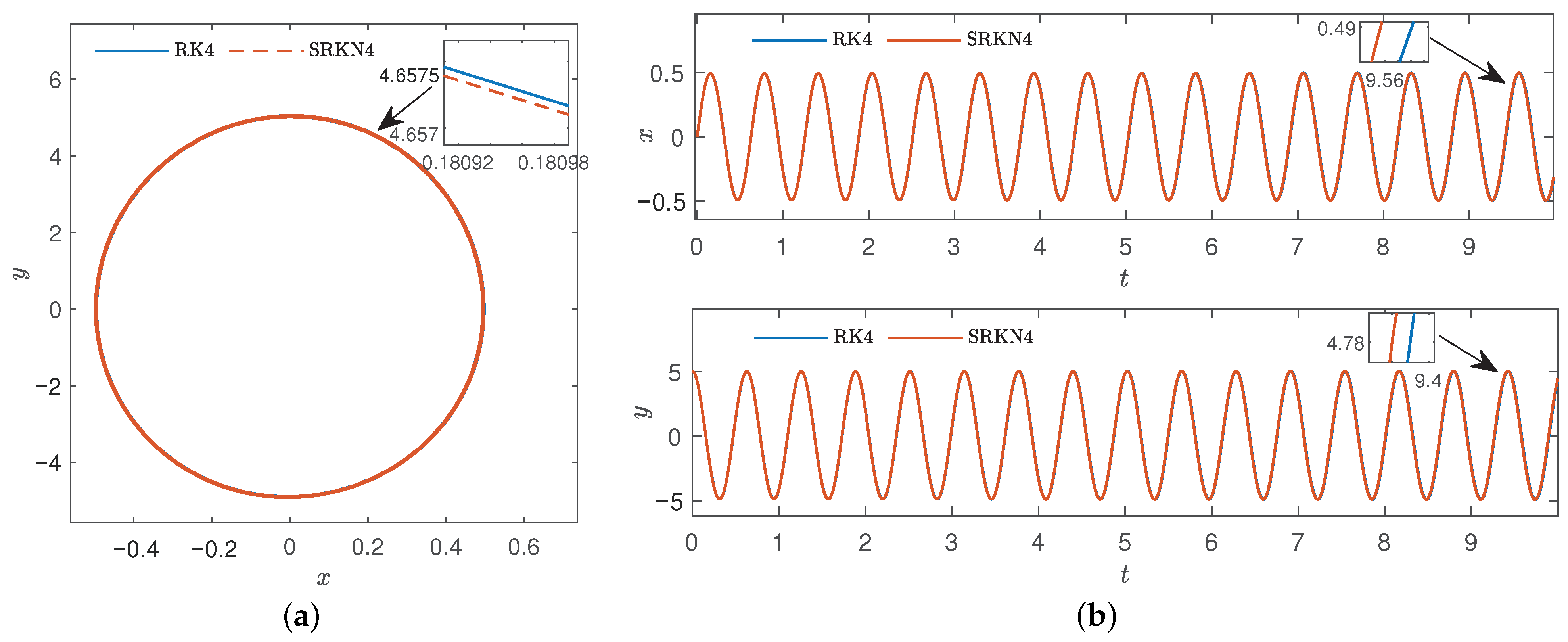
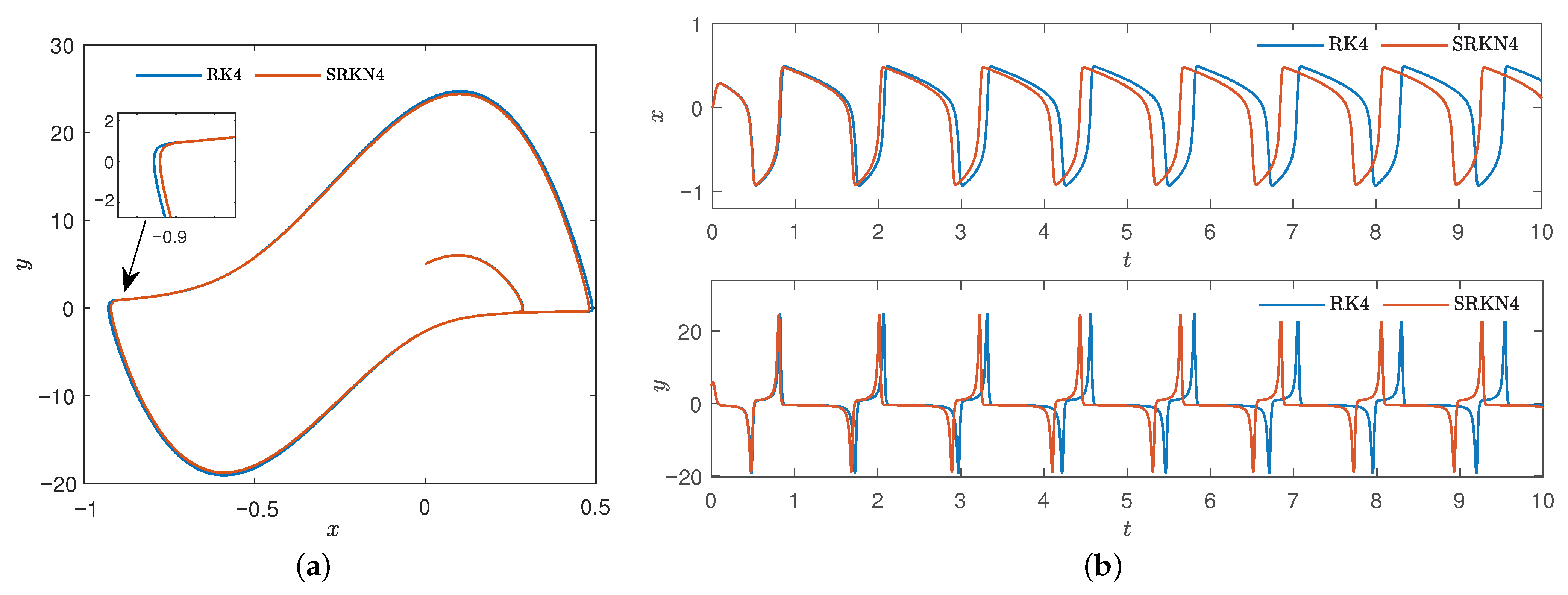
3.4.2. Runge–Kutta Method and Symplectic Runge–Kutta–Nyström Method

a. ξ = 0.1
As in Section 3.3.2, when ξ = 0.1 , we analyzed the classic four-order Runge–Kutta method and four-order symplectic Runge–Kutta–Nyström method.
Case 1: h = 0.01 .
Here, set the starting point to ( 0 , 5 ) , given ξ = 0.1 , Δ 1 = 16 , Δ 2 = 8 , ω 0 = 10 , and set the step h = 0.01 , the number of iterations is n = 10,000. Then, the comparison of classic four-order Runge–Kutta method and four-order symplectic Runge–Kutta–Nyström phase trajectories and displacement component changes of time series were obtained in Figure 10.
From Figure 10, it can be found that both methods preserved the structure and symmetry of system well, but the computation time of symplectic method is faster than that of non-symplectic method. For further analysis, we increased the step.
Case 2: h = 0.09 .
As in case 1, we only increase the step h, let h = 0.09 , the number of iterations is n = 10,000, and other conditions remain unchanged, resulting in Figure 11.
According to Figure 11, when the step increased, the trajectory trend obtained by Runge–Kutta method will be quickly decoupled from the periodic one and instantaneously collapse, and the structure cannot be preserved. However, the stability properties of the periodic orbit and symmetry are preserved by the symplectic Runge–Kutta–Nyström method. Then, we calculate the Hamiltonian under classic four-order Runge–Kutta method and four-order symplectic Runge–Kutta–Nyström method when ξ is small enough, as shown in Table 3.
Therefore, a comparison diagram of error trends of different methods is presented, as shown in Figure 12.
When ξ is sufficiently small, the Hamiltonian of symplectic Runge–Kutta method still remain within a certain range, however, the classic Runge–Kutta method diverges and does not preserve the structure. Through the comparison, the symplectic method is shown to have a higher coincidence with the exact solution and the structure is preserved.
b. ξ = 20
In order to further illustrate the superiority of the symplectic method, we set ξ = 20 and adjust the step h based on this, also consider the description of two cases.
Case 1: h = 0.001 .
When the value of ξ is very large, given ξ = 20 , likewise Δ 1 = 16 , Δ 2 = 8 , ω 0 = 10 , the number of iterations n = 10,000, set the step h = 0.001 , Figure 13 shows the phase plane and time traces between the classic four-order Runge–Kutta method and four-order symplectic Runge–Kutta–Nyström method.
Obviously, from Figure 13, symplectic method is more reliable in structure preserving performance and convergent faster than non-symplectic method.
Case 2: h = 0.02 .
As in case 1, we only increase the step h, and let h = 0.02 , other conditions remain unchanged, resulting in Figure 14.
According to Figure 14, when the step increased, the trajectory trend obtained by classic Runge–Kutta method will be quickly decoupled from the periodic one and instantaneous collapsed.
Through case 1 and case 2 of Section 3.4.1 and Section 3.4.2, under ξ = 0.1 and ξ = 20 , in the case of long-time and large step numerical integration, symplectic method can still better maintain the characteristics of the system than non-symplectic method. That is, the symplectic method can preserve the structure well. In particular, when the perturbation term is small, the system tends to be a Hamiltonian system, and the symplectic method can maintain the symmetry of the system.

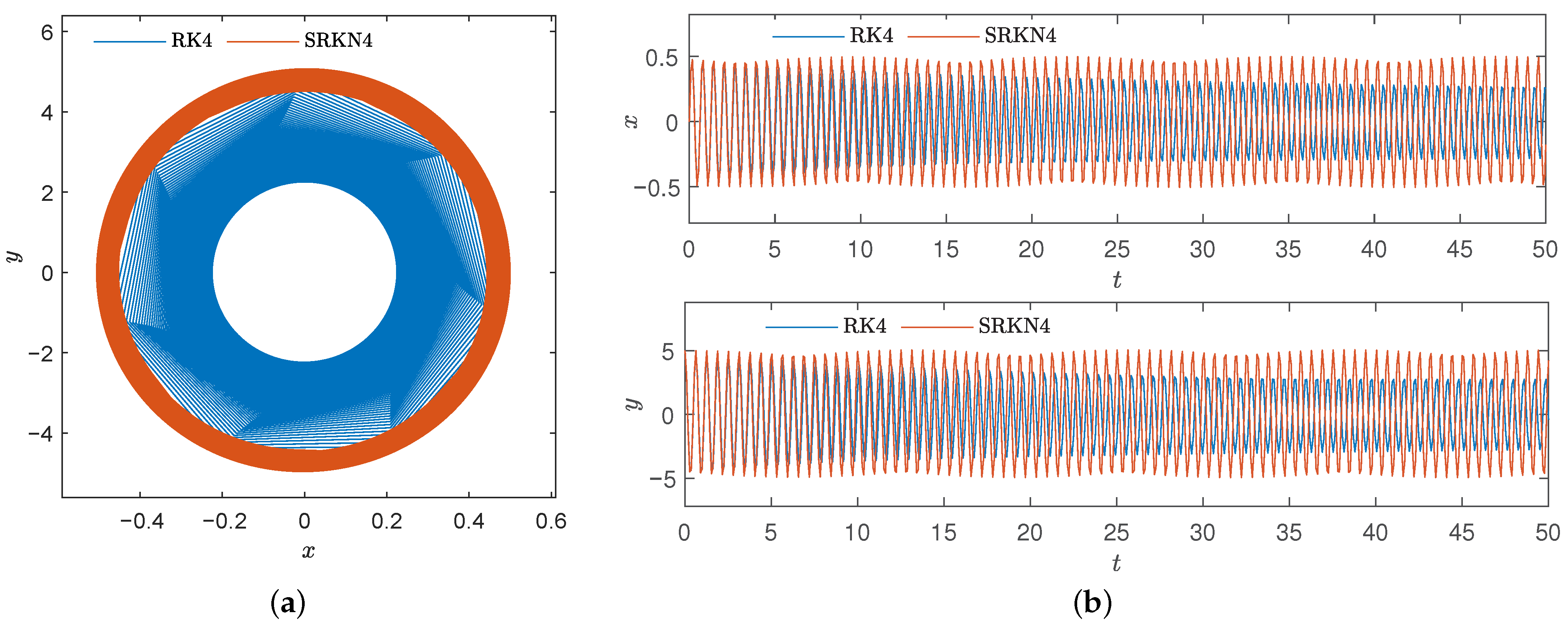
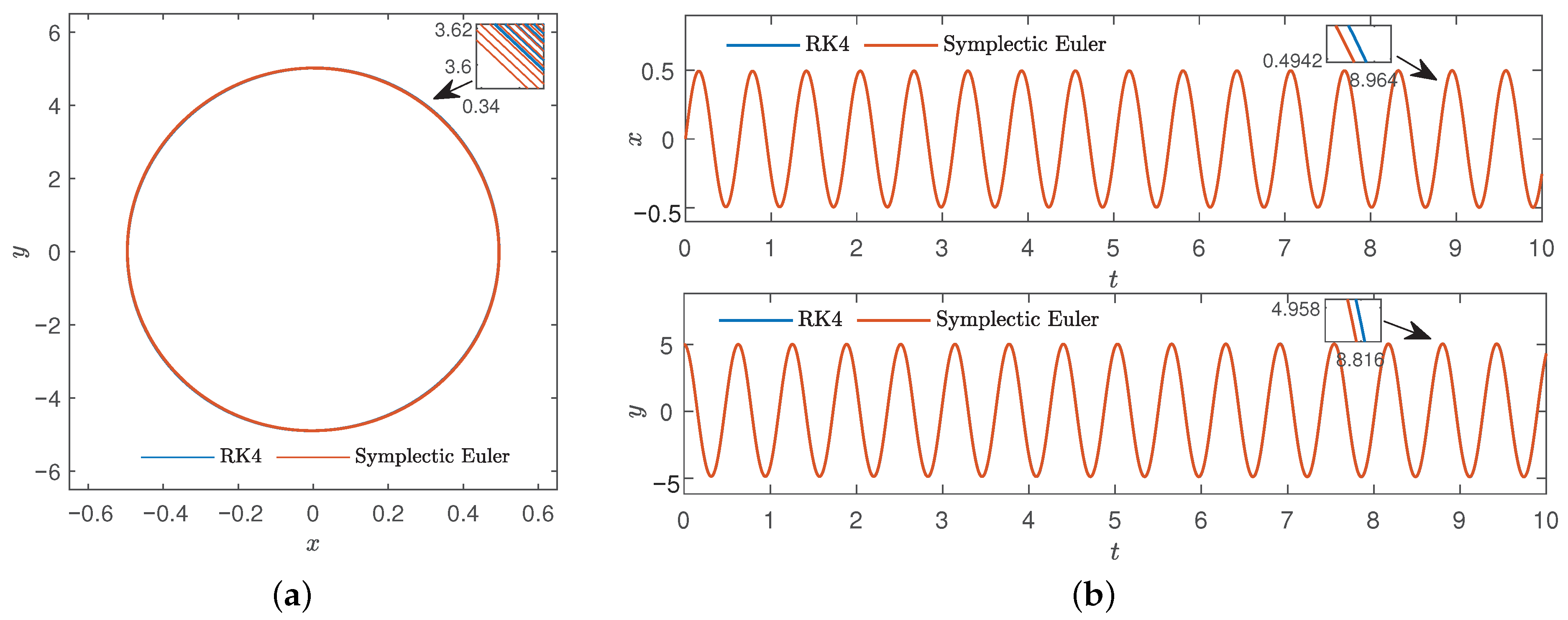
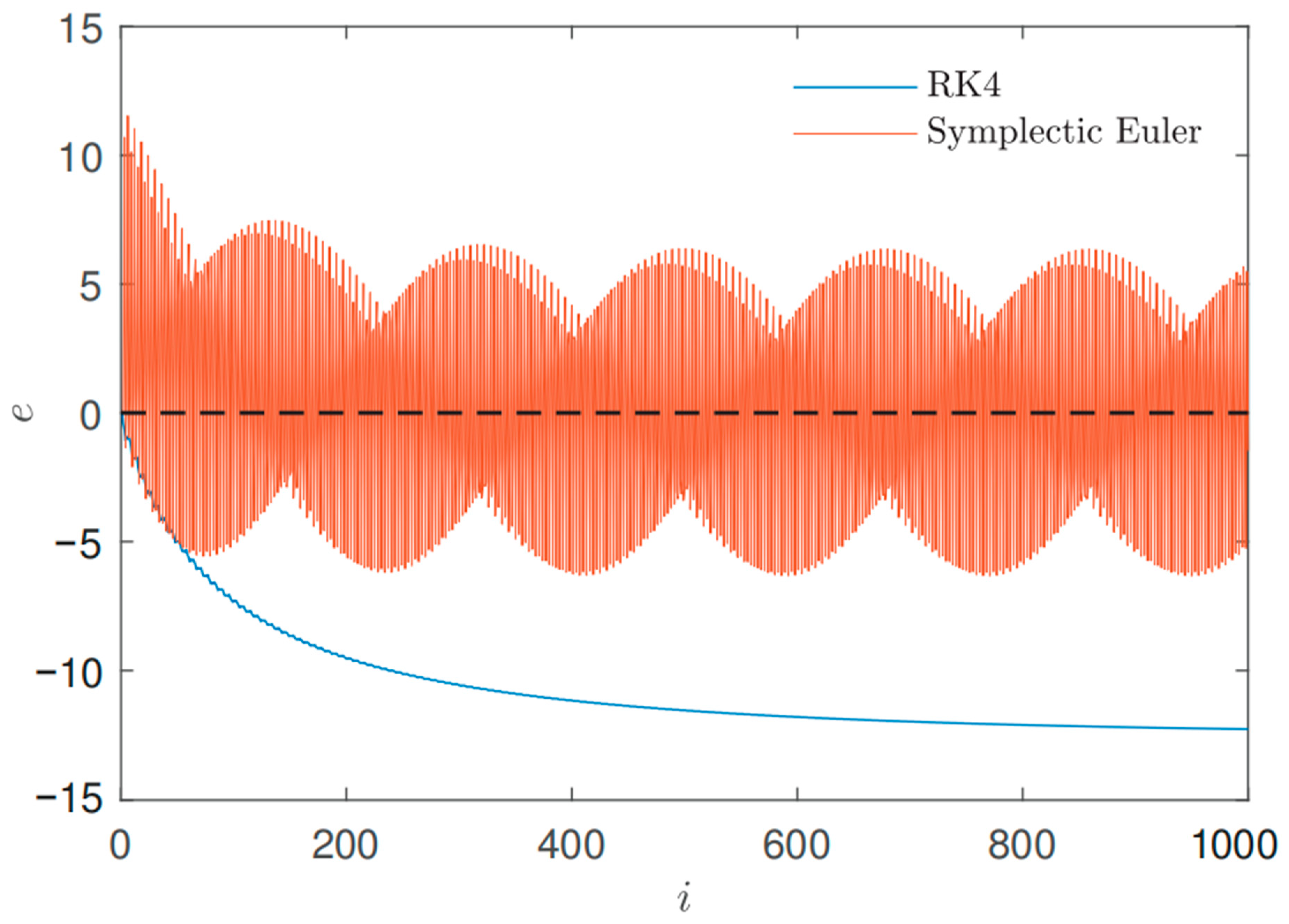
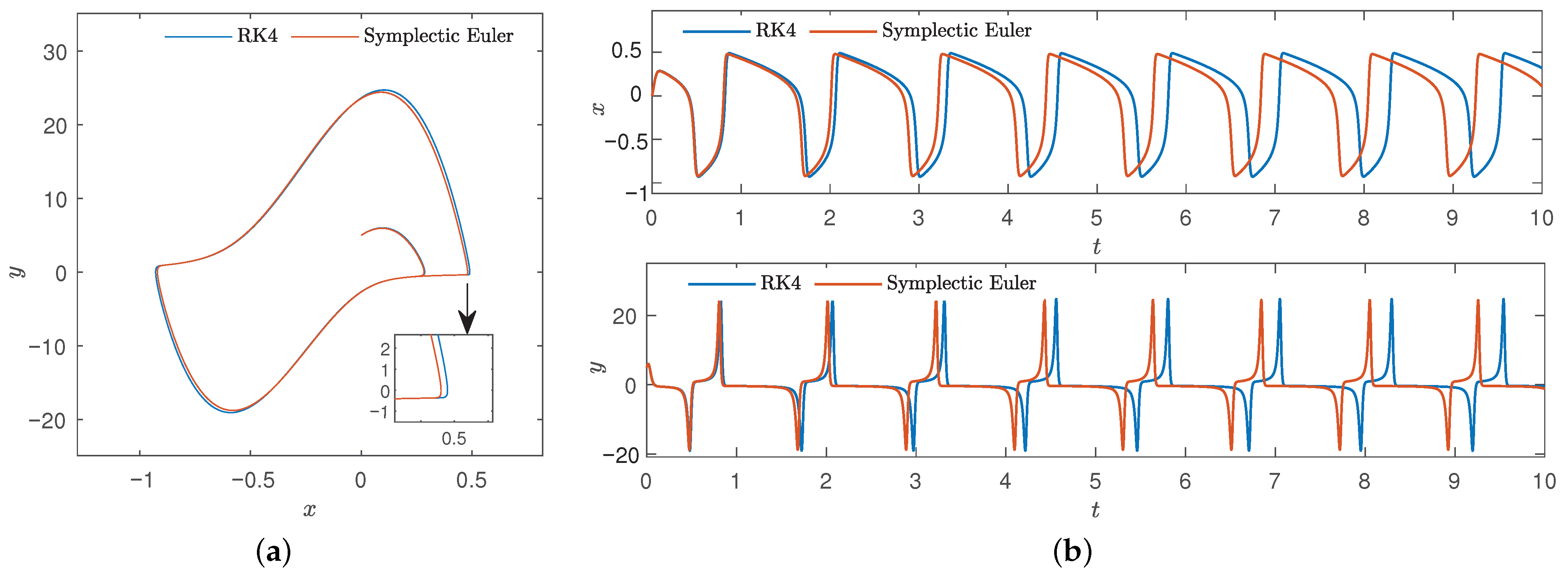
3.4.3. Symplectic Euler Method and Four-Order Runge–Kutta Method

In the previous sections, we compare the symplectic and classical methods of Euler method and Runge–Kutta method, respectively. In this section, we consider comparing the symplectic Euler method with the classical four-order Runge–Kutta method.
a. ξ = 0.1
As in Section 3.3.2, when ξ = 0.1 , we analyzed the classic four-order Runge–Kutta method and symplectic Euler method.
Case 1: h = 0.001 .
Set the starting point to ( 0 , 5 ) , given ξ = 0.1 , Δ 1 = 16 , Δ 2 = 8 , ω 0 = 10 , and set the step h = 0.001 , the number of iterations is n = 10,000. Then, the comparison of classic four-order Runge–Kutta method and symplectic Euler phase trajectories and displacement component changes of time series were obtained in Figure 15.
From Figure 15, it can be found that both methods preserved the structure and symmetry of the system well, but the computation time of symplectic Euler method is faster than that of classic Runge–Kutta method. For further analysis, we increased the step.
Case 2: h = 0.1 .
As in case 1, we only increase the step h, let h = 0.1 , the number of iterations is n = 10,000 and other conditions remain unchanged, resulting in Figure 16.
According to Figure 16, when the step increases, the trajectory trend obtained by the classical Runge–Kutta method will be decoupled from the periodic trend, resulting in instantaneous collapse and the structure cannot be preserved. Meanwhile, the symplectic Euler method did not structure preserved well in the end, but it did not collapse, nor did it collapse in time. Then, we calculate the Hamiltonian under classic four-order Runge–Kutta method and symplectic Euler method when ξ is small enough, as shown in Table 4.
Then, comparison diagram of error trends of different methods is presented, resulting in Figure 17.
The ξ is sufficiently small, the Hamiltonian of the classic Runge–Kutta method diverges and does not preserve the structure, and the errors produced by symplectic Euler method are also larger, but compared with Runge–Kutta method, it is still remain within a certain range.
b. ξ = 20 , h = 0.001
In order to further illustrate the contrast between symplectic Euler and classical Runge–Kutta method. When the value of ξ is very large, given ξ = 20 , likewise Δ 1 = 16 , Δ 2 = 8 , ω 0 = 10 , the number of iterations n = 10,000, set the step h = 0.001 , Figure 18 shows the phase plane and time traces between the classic four-order Runge–Kutta method and symplectic Euler method.
From Figure 18, symplectic Euler method is more reliable in structure preserving performance and convergent faster than classic four-order Runge–Kutta method. Furthermore, In this case, we did not compare the methods when the steps increased, so it was unnecessary to preserve the structure of the system. Moreover, the above method has obvious advantages in speed and has also achieved victory in structure preserving.

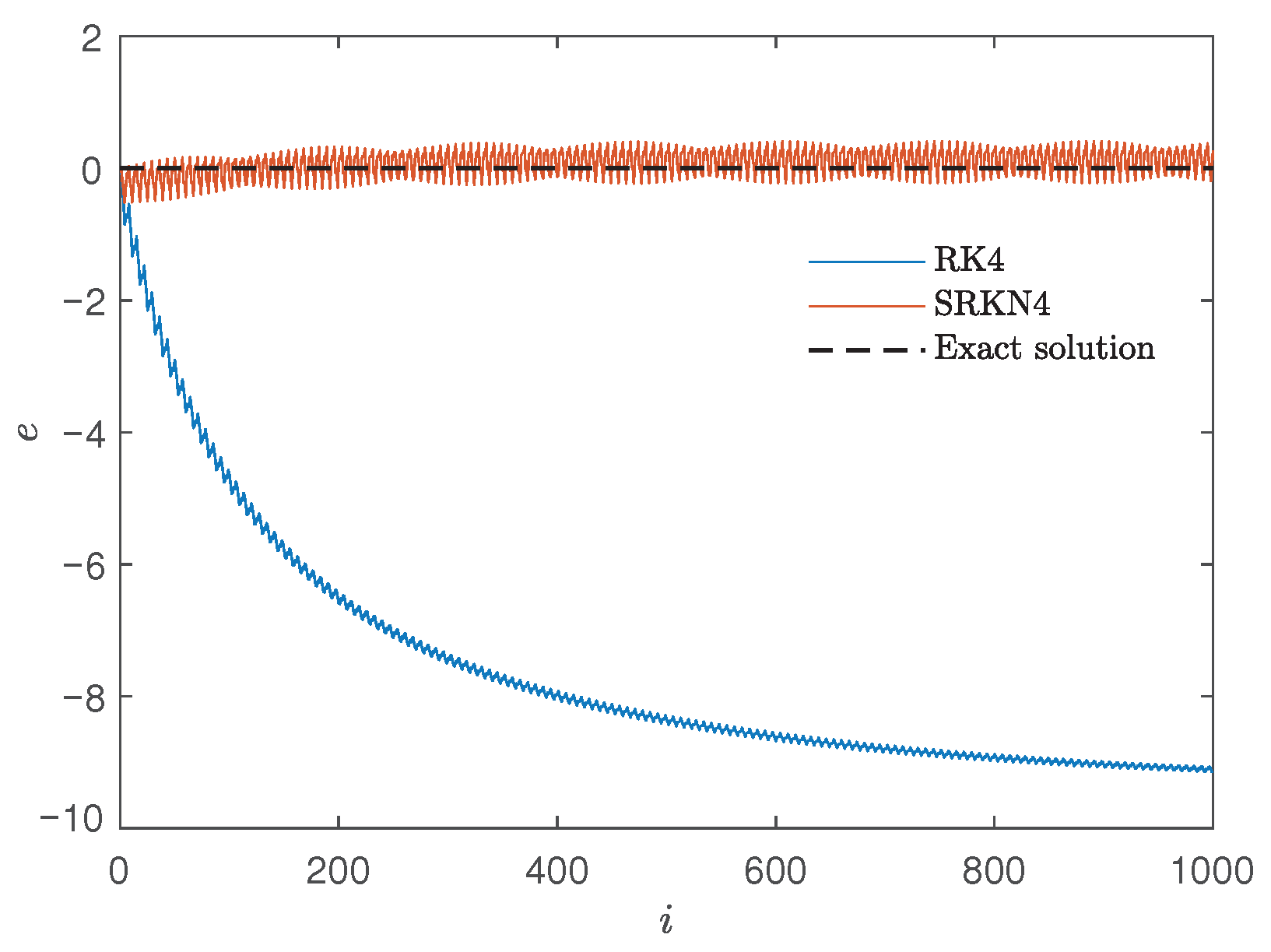
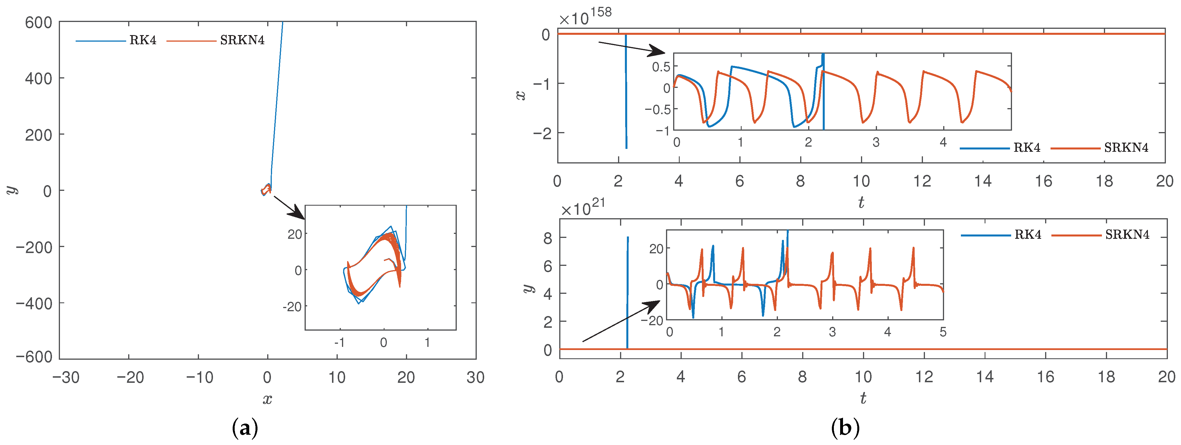
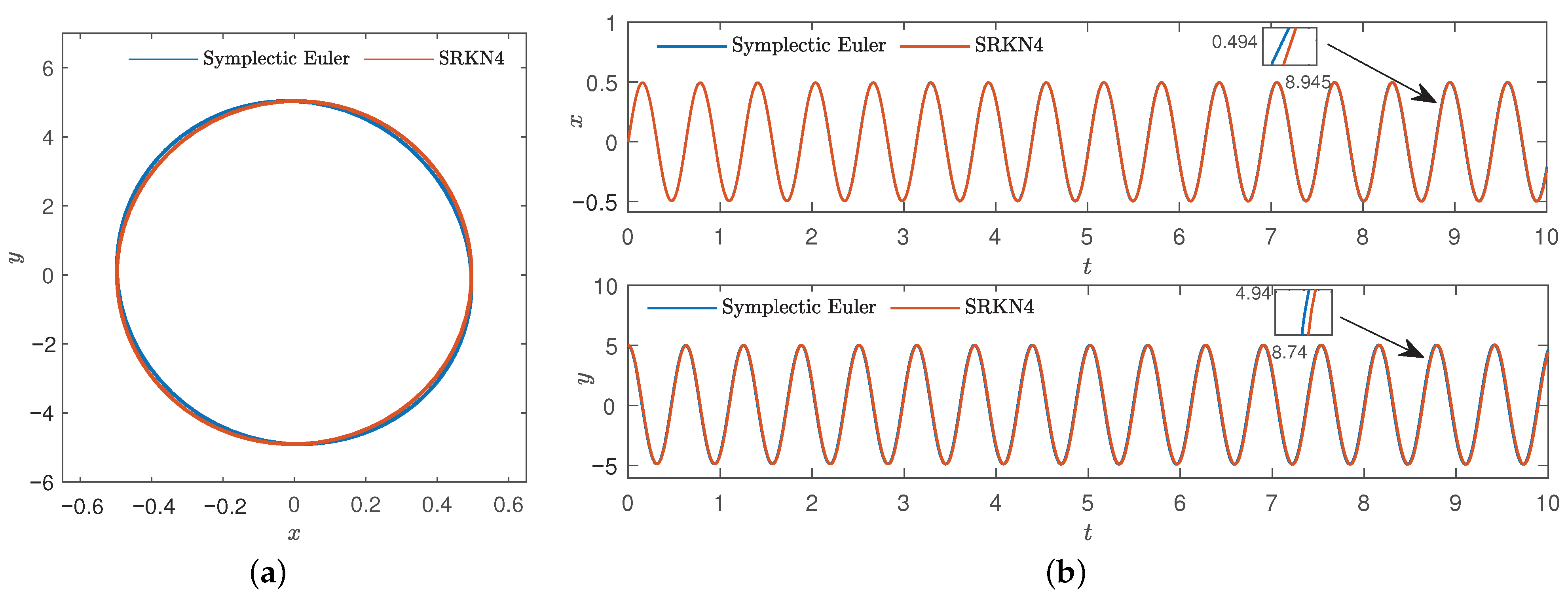
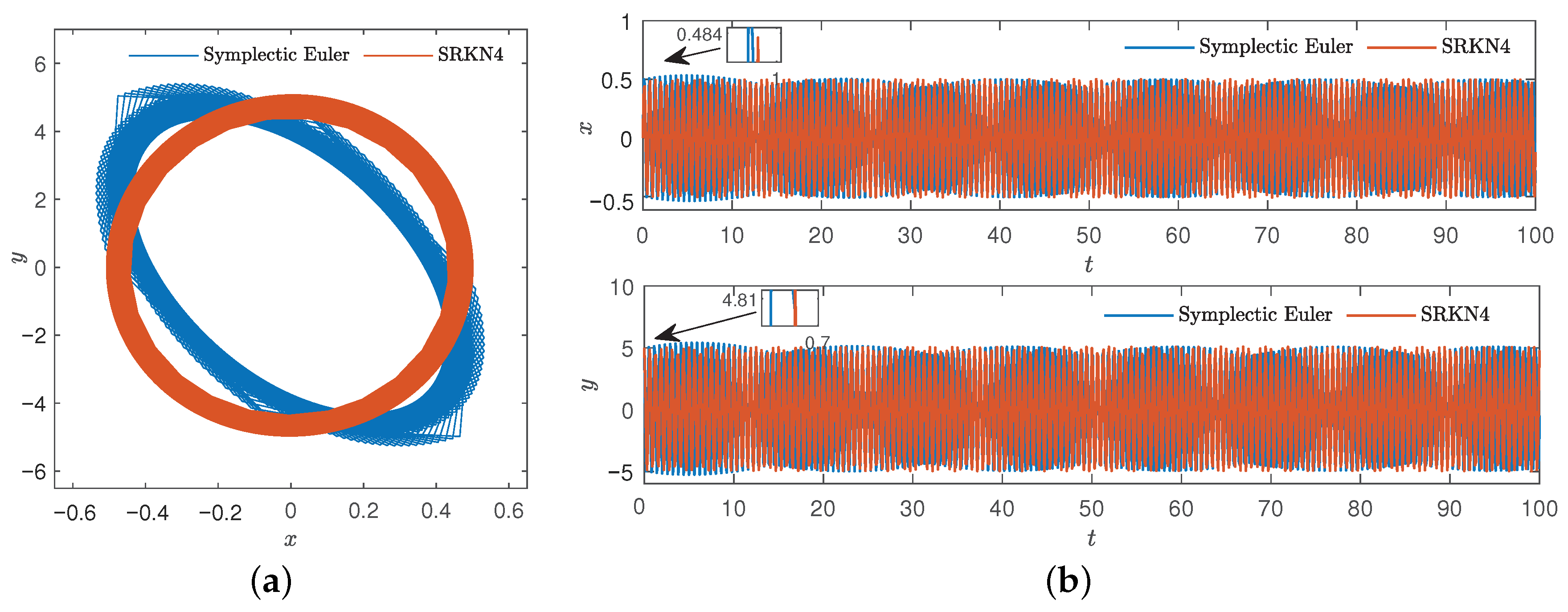
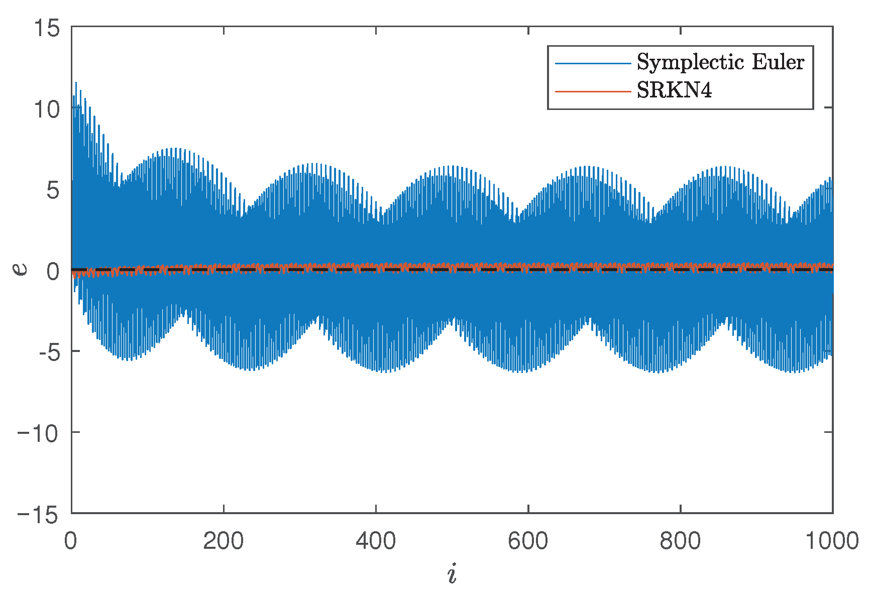
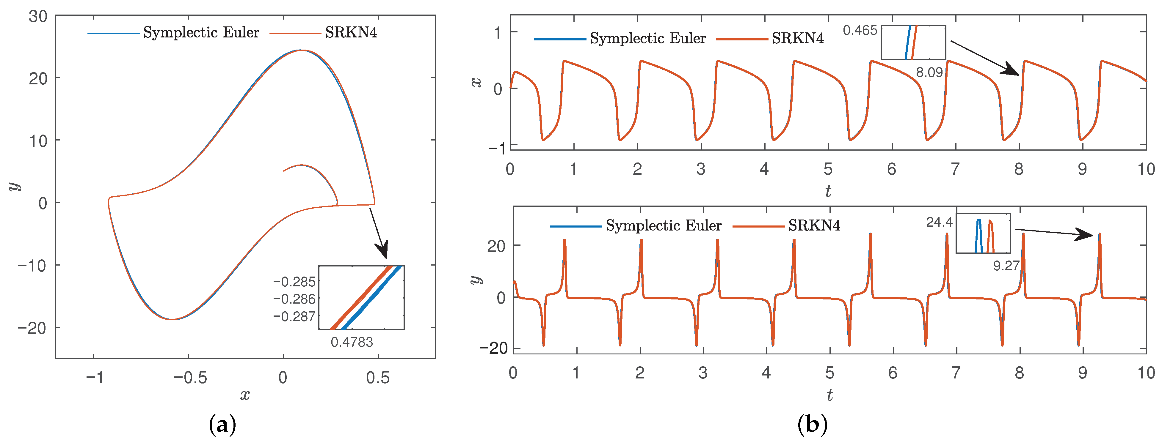
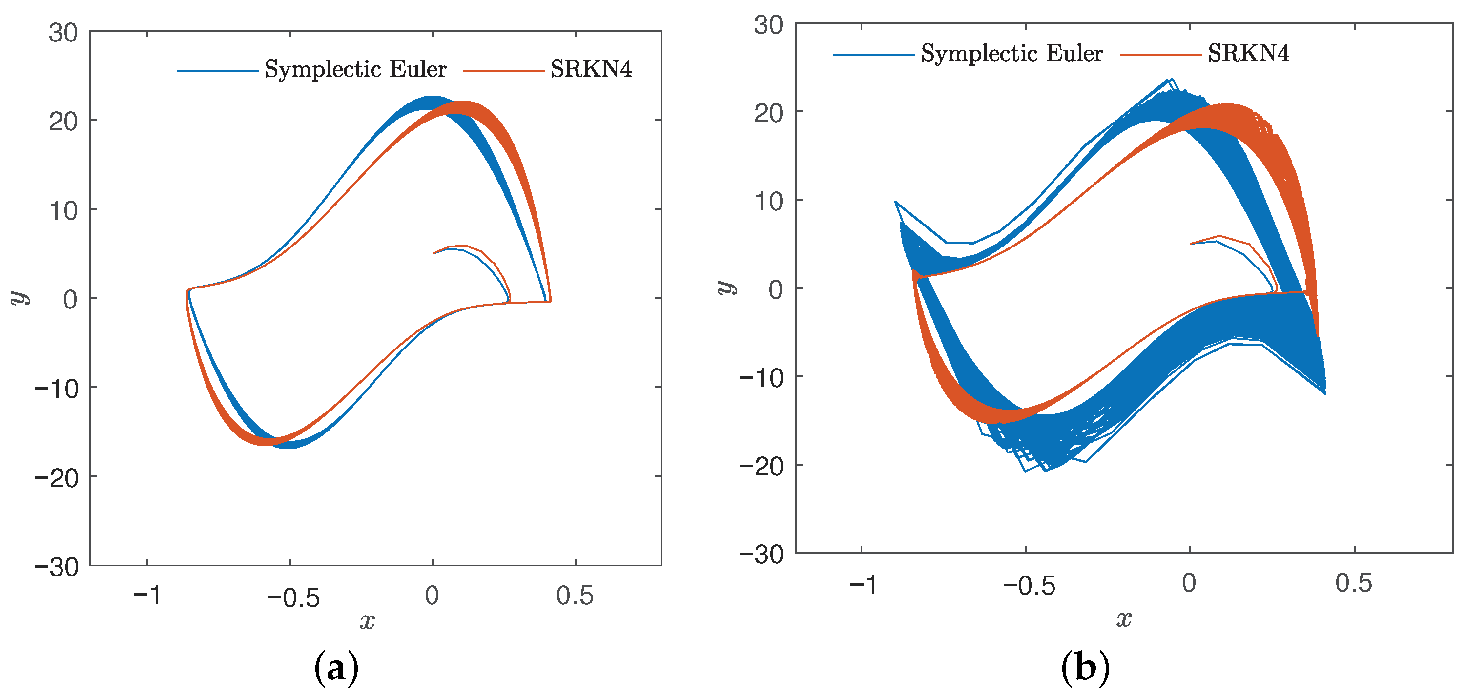
3.4.4. Symplectic Euler Method and Symplectic Runge–Kutta–Nyström Method

a. ξ = 0.1
When ξ = 0.1 , we analyzed the symplectic Euler method and four-order symplectic Runge–Kutta–Nyström method.
Case 1: h = 0.01 .
Similarly, set the starting point to ( 0 , 5 ) , given ξ = 0.1 , Δ 1 = 16 , Δ 2 = 8 , ω 0 = 10 , and set the step h = 0.01 , the number of iterations is n = 10,000. Then, the comparison of the symplectic Euler and four-order symplectic Runge–Kutta–Nyström phase trajectories and displacement component changes of time series were obtained in Figure 19.
From Figure 19, it can be found that both methods preserved the structure and symmetry of system well, but the computation time of symplectic Euler method is faster than that of symplectic Runge–Kutta–Nyström method. For further analysis, we increased the step.
Case 2: h = 0.1 .
As in case 1, we only increase the step h, let h = 0.1 , the number of iterations is n = 10,000, and other conditions remain unchanged, resulting in Figure 20.
According to Figure 20, when the step increases, the trajectory trend of the symplectic Euler method is decoupled from the periodic one, and the structure cannot be preserved. However, symplectic Runge–Kutta–Nyström preserves symmetry and structure, while the symplectic Euler method has an advantage in calculating speed. Then, we calculate the Hamiltonian under symplectic Euler method and four-order symplectic Runge–Kutta–Nyström method when ξ is small enough, as shown in Table 5.
Therefore, a comparison diagram of error trends of different methods is presented, as shown in Figure 21.
From above, when ξ is sufficiently small and step increases, the symplectic Runge–Kutta–Nyström method’s Hamiltonian remains within a certain range, while the symplectic Euler method diverges, but remains within a certain range (albeit a large one). By comparison, the symmetry and structure of the symplectic Runge–Kutta–Nyström method are better under the condition of small perturbation and large step.
b. ξ = 20
To further illustrate the conditions of symplectic method and the characteristics of each methods, we set ξ = 20 and adjust the step h based on this, also consider the description of two cases.
Case 1: h = 0.001 .
When the value of ξ is large, given ξ = 20 , likewise Δ 1 = 16 , Δ 2 = 8 , ω 0 = 10 , the number of iterations n = 10,000, set the step h = 0.001 , Figure 22 shows the phase plane and time traces between the symplectic Euler method and four-order symplectic Runge–Kutta–Nyström method.
From Figure 22, the symplectic Euler method and symplectic Runge–Kutta–Nyström method both preserve the structure of the system well, but the symplectic Euler method is superior in computing speed by comparison.
Case 2: Large step.
As in case 1, we only increase the step h, and make the step change constantly, other conditions remain unchanged, resulting in Figure 23.
According to Figure 23, it can be seen from the figure that when the step increases, h = 0.01 , the symplectic Euler method and the four-order symplectic Runge–Kutta–Nyström method do not well preserve the system structure. When the step continues to increase and h = 0.0159 , the trajectory trend obtained by the symplectic Euler method is decoupled from the periodic trend first, and the system structure is no longer preserved. Meanwhile, if the step size continues to increase, both methods can no longer preserve the system structure.
Through the discussion of various cases in Section 3.4, we conclude that the symplectic method maintains the characteristics of the system better than the non-symplectic method in the case of large and long numerical integrals over long time. In particular, when the perturbation is very small, the system tends to be Hamiltonian, and symplectic methods can preserve the symmetry and structure of the system better than classic methods. Meanwhile, when the method is not confined to the comparison of the two symplectic methods, the perturbation is very small, the symplectic methods do not differ much. When the perturbation becomes larger, the step becomes the key to influence the numerical integration, that is, when the step is larger, the symplectic Runge–Kutta–Nyström method wins, but the computational speed of the symplectic Euler method is better than that of the symplectic Runge–Kutta–Nyström method.

4. Primary and Subharmonic Simultaneous Resonance of Forced van der Pol Oscillator

Due to the interaction between self-excited oscillation and forced oscillation, complex dynamic phenomena appear in the van der Pol non-autonomous system with a sinusoidal forcing term. Many resonance phenomena occur in non-autonomous dynamical systems under forced excitation, especially under multi-frequency excitation. In this section, the primary and subharmonic simultaneous resonances of van der Pol oscillators are studied.

4.1. First-Order Approximate Solution of Primary and Subharmonic Simultaneous Resonance

A memristor circuit based on forced van der Pol oscillator system excited by multiple frequencies can be described as system (4). The parameters are specified as follows: ω 1 = ω 0 + ξ ψ 1 , ω 2 = 3 ω 0 + ξ ψ 2 , A 1 = ξ f , f = O ( 1 ) , ψ 1 = O ( 1 ) , ψ 2 = O ( 1 ) , the system (4) changes into
x ¨ + ω 0 2 x = ξ ( 1 Δ 1 x 2 Δ 2 x ) x ˙ + f cos ω 1 t + A 2 cos ω 2 t
where, ω 0 is the natural frequency of the linearized system (2). A multi-scale method [59] is applied to study the first-order approximate solution of the system. Suppose that the solution form of the system (23) is as follows:
x ( t ) = x 0 ( T 0 , T 1 ) + ξ x 1 ( T 0 , T 1 )
where, time scales are T 0 = t , T 1 = ξ t , and substituting Equation (24) into Equation (23), by comparing the same power of, a system of partial differential equations is obtained:
D 0 2 x 0 + ω 0 2 x 0 = A 2 cos ( 3 ω 0 T 0 + ψ 2 T 1 )
D 0 2 x 1 + ω 0 2 x 1 = 2 D 0 D 1 x 0 + f cos ( ω 0 T 0 + ψ 1 T 1 ) + 2 D 0 ( 1 Δ 1 x 0 2 Δ 2 x 0 ) x 0
Then, the general solution of Equation (25) is x 0 ( T 0 , T 1 ) = a ( T 1 ) cos ω 0 T 0 + b ( T 1 ) + A 2 ω 0 2 ω 1 2 cos ( 3 ω 0 T 0 + ψ 2 T 1 ) and it can also be written as plural form:
x 0 ( T 0 , T 1 ) = K ( T 1 ) e j ω 0 T 0 + P e j ( 3 ω 0 T 0 + ψ 2 T 1 ) + c
where, K ( T 1 ) = a ( T 1 ) e j b ( T 1 ) 2 , P = A 2 2 ( ω 0 2 ω 1 2 ) , c is the conjugate of all the preceding terms. a ( T 1 ) , b ( T 1 ) are slowly varying amplitude and phase, respectively. Substitute Equation (27) into Equation (26), eliminate the secular term and separating real and imaginary parts. The differential equations satisfied by slowly varying amplitude a ( T 1 ) and phase b ( T 1 ) are obtained
D 1 a = ξ ψ 1 a 2 B 24 ω 0 sin ( 3 b ψ 2 T 1 ) f 2 ω 0 sin ( b ψ 1 T 1 ) ξ ψ 1 a 6 a D 1 b = ξ a 6 ω 0 + ξ Δ 1 a P 2 12 ω 0 + ξ Δ 1 a 2 P 6 ω 0 cos ( 3 b ψ 2 T 1 ) f 2 ω 0 cos ( b ψ 1 T 1 ) + ξ Δ 1 a 3 6 ω 0
Consequently, the first-order approximate solution of system (23) can be expressed as
x 0 ( t ) = 2 P cos ( ω 2 t ) + a cos ( ω 0 t + b )
where, a and b determined by the Equation (28).

4.2. Steady Solution and Its Stability Conditions

From above, the necessary conditions for the existence of steady solutions are b ψ 1 T 1 and 3 b ψ 2 T 1 are constants from Equation (27), where ψ 2 = 3 ψ 1 , ω 2 = 3 ω 1 . In other words, the steady solution of primary and subharmonic simultaneous resonance can be obtained only when the two excitation frequencies are sufficient to a specific multiple relationship. Let 3 ψ = 3 ψ 1 = ψ 2 , b ψ 1 T 1 = γ , then Equation (28) can be written as autonomous differential equations:
D 1 a = ξ ψ 1 a 2 P 24 ω 0 sin ( 3 γ ) f 2 ω 0 sin ( γ ) ξ ψ 1 a 6 a D 1 b = ξ a 6 ω 0 + ξ Δ 1 a P 2 12 ω 0 + ξ Δ 1 a 2 P 6 ω 0 cos ( 3 γ ) f 2 ω 0 cos ( γ ) + ξ Δ 1 a 3 6 ω 0
The corresponding first-order approximate solution becomes
x ( t ) = a cos ( ω 1 t + γ ) + 2 P cos ( ω 2 t )
where, ω 2 = 3 ω 1 . To verify the accuracy of the first-order approximate solution of Equation (31). The Runge–Kutta method with variable step length is used to calculate the system (4), and it is compared with the first-order approximate solution of Equation (31). According to the above section, let ξ = 0.1 , Δ 1 = 16 , Δ 2 = 8 , ω 0 = 2.5 , ω 2 = 3 ω 1 = 7.5 , A 1 = 0.2 , A 2 = 2 and the simulation duration t = 50 . The transient response is called when the initial time t ( 0 , 20 ) . Figure 24 shows the transient responses times.
Then, let the last time t ( 20 , 50 ) , and the response amplitude as the steady-state amplitude, take the initial value ( a 0 , γ 0 ) = ( 0.72 , 1.51 ) , the steady-state response is shown in Figure 25.
As can be seen from Figure 24 and Figure 25, when ω 2 = 3 ω 1 , the approximation between numerical solution and analytical solution is better, and the multiple solutions and unstability phenomena of the system are mainly dominated by a cos ( ω 1 t + γ ) of system (31). Therefore, in the subsequent study of the dynamical behaviors of system (4), only ω 1 in the external excitation needs to be studied.

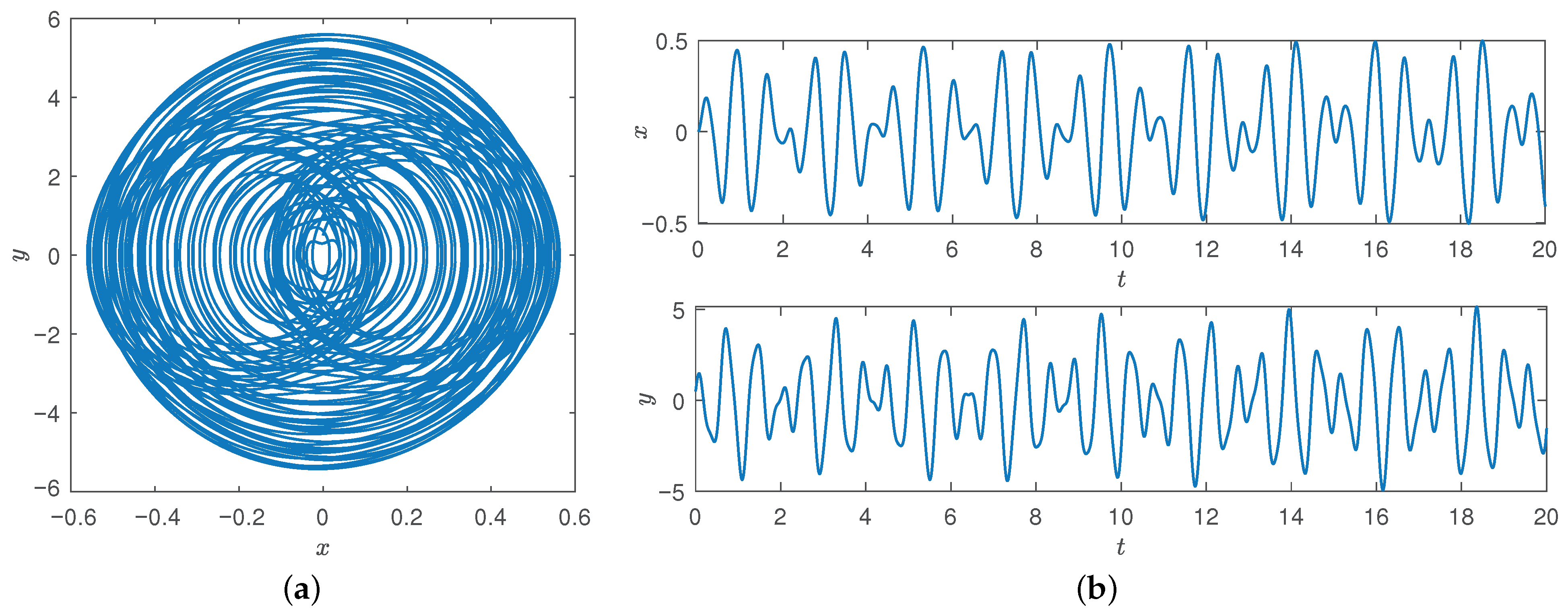
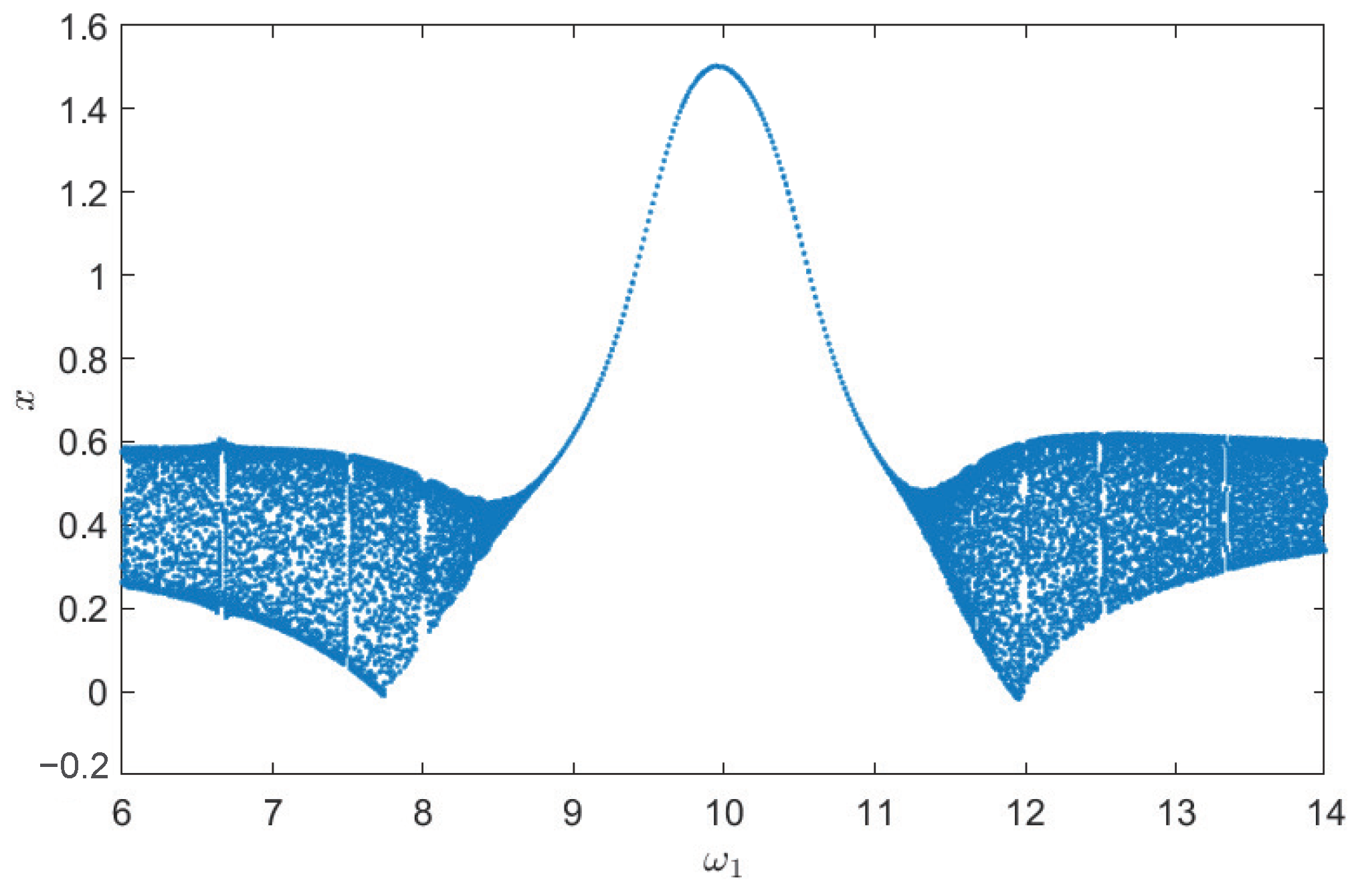
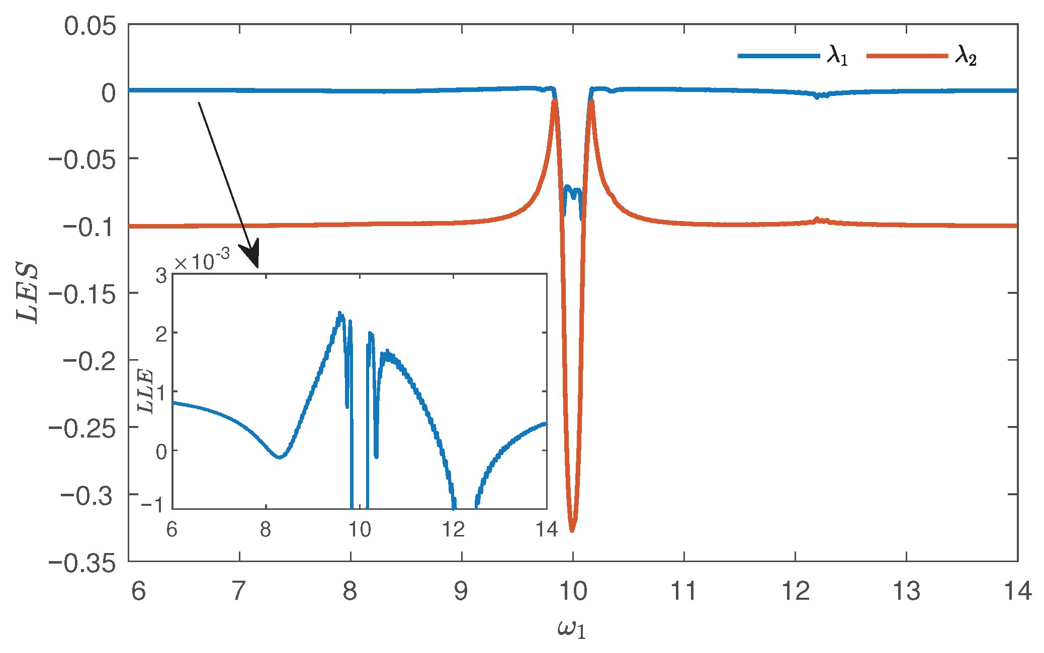
4.3. Analysis of Chaotic Dynamics

In the resonance analysis in Section 4.1 and Section 4.2, we get ω 2 = 3 ω 1 , then the system (4) becomes
x ˙ = y y ˙ = ξ ( 1 Δ 1 x 2 Δ 2 x ) y ω 0 2 x + A 1 cos ( ω 1 t ) + A 2 cos ( 3 ω 1 t )
Then, the system (32) will have different and complex dynamical behaviors when changing ξ , and we will analyze these dynamical behaviors under different ξ .

4.3.1. Dynamical Behaviors of ξ = 0.1

The 2D nonlinear non-autonomous systems can produce chaotic behaviors, and chaos will occur when the nonlinearity of a memristor circuit based on its van der Pol oscillators is strong. When ξ = 0.1 , with Δ 1 = 16 , Δ 2 = 8 , ω 0 = 10 , A 1 = 12 , A 2 = 8 and ω 1 = 7.1 , the initial value x , y = 0 , 0.5 is selected. The chaotic attractor and time series are shown in Figure 26.
Under the same parameters, when control parameters ω 1 6 , 14 , the bifurcation diagram of the system (32) is shown in Figure 27.
Figure 27 shows a bifurcation diagram of x as a function of ω 1 , and the system undergoes a variety of dynamical behaviors. In addition, to further verify the existence of chaos, we give the Lyapunov exponential spectrum and the largest Lyapunov exponential trend diagram in Figure 28.
The Lyapunov exponential spectrum in Figure 28 shows rich dynamical behaviors and shows that the largest Lyapunov exponential is positive. The largest Lyapunov exponential diagram has the same results as the bifurcation diagram. These results also agree with the analysis of van der Pol oscillators.

4.3.2. Dynamical Behaviors of ξ = 5

Similarly, when ξ = 5 , with Δ 1 = 16 , Δ 2 = 8 , ω 0 = 10 , A 1 = 10 , A 2 = 5 and ω 1 = 3.7 , the initial value x , y = 0 , 0.5 is selected. The chaotic attractor and zoom in on Poincaré section are shown in Figure 29.
From Figure 29, the chaotic attractor generates a type relaxation oscillator configuration, and the continuously dense point shows chaotic behavior. Then, we change the value of ω 1 to get the phase diagram and Poincaré section with different parameters and the states of periodic 1, periodic 2 and periodic3 can be obtained, as shown in Figure 30.
When control parameters ω 1 0 , 9 , the bifurcation diagram of the system (32) is shown in Figure 31.
From above, it can be seen that many narrow periodic windows are embedded in chaotic regions, and it contains rich dynamical behaviors. Thus, the forced parameter ξ and ω 1 can be used to tune the memristor circuit to different chaotic or periodic oscillations.

5. Conclusions

A memristor circuit based on its van der Pol oscillator is introduced, and the stability and dynamic characteristics of memristor circuit are studied. Meanwhile, the differences of the van der Pol oscillation model of memristor between the Euler method and symplectic Euler method, four-order Runge–Kutta method and four-order symplectic Runge–Kutta–Nyström method, symplectic Euler method and four-order Runge–Kutta method, symplectic Euler method and four-order symplectic Runge–Kutta–Nyström method in preserving symmetry and structure are compared from theoretical and numerical simulation: The symplectic scheme can better simulate the oscillate process of the oscillator and keep the conservation of the harmonic oscillator accurately in the time domain for a long time. Secondly, the analytic solution of the primary and subharmonic (1/3 order) simultaneous resonance of the van der Pol oscillation system is obtained by using the multi-scale method, and the stability condition of the steady solution is obtained by using Lyapunov stability theory. Finally, the dynamical behaviors of the system is studied from the resonance relationship, which is helpful to understand the oscillation characteristics of other nonlinear oscillation problems in the form of van der Pol equation later. In the future, we will consider comparing more structure preserving symplectic methods with classical integral methods to demonstrate the advantages of symplectic methods, and which will be used in aerospace, nanomaterials and other applications. Meanwhile, we will further study the memristor system on the electronic circuit, and the global dynamics and infinite behaviors of the system are considered.

Author Contributions

Conceptualization, Z.W. and B.Y.; methodology, Z.W. and B.Y.; software, H.T. and J.L.; validation, Z.W., B.Y., H.T. and J.L.; formal analysis, B.Y., H.T. and J.L.; writing—original draft preparation, B.Y. and H.T.; writing—review and editing, Z.W., B.Y., H.T. and J.L. All authors have read and agreed to the published version of the manuscript.

Funding

This research was funded by the Natural Science Basic Research Program of Shaanxi (2021JM-533, 2021JQ-880, 2020JM-646), the Innovation Capability Support Program of Shaanxi (2018GHJD-21), the Science and Technology Program of Xi’an (2019218414GXRC020CG021-GXYD20.3), the Support Plan for Sanqin Scholars Innovation Team in Shaanxi Province of China, the Scientific Research Program Funded by Shaanxi Provincial Education Department (21JK0960), the Youth Innovation Team of Shaanxi Universities and the Scientific Research Foundation of Xijing University (XJ21B01), the Scientific Research Foundation of Xijing University (XJ210203).

Institutional Review Board Statement

Not applicable.

Informed Consent Statement

Not applicable.

Data Availability Statement

Not applicable.

Acknowledgments

The authors acknowledge the referees and the editor for carefully reading this paper and giving many helpful comments. The authors also express their gratitude to the reviewers for their insightful comments.

Conflicts of Interest

The authors declare no conflict of interest.

References

  1. Van Der Pol, B. VII. Forced oscillations in a circuit with non-linear resistance. (Reception with reactive triode). Lond. Edinb. Dublin Philos. Mag. J. Sci. 1927, 3, 65–80. [Google Scholar] [CrossRef]
  2. Kpomahou, Y.J.F.; Miwadinou, C.H.; Agbokpanzo, R.G.; Hinvi, L.A. Nonlinear dynamics of a RLC series circuit modeled by a generalized van der Pol oscillator. Int. J. Nonlinear Sci. Numer. Simul. 2021, 22, 479–494. [Google Scholar] [CrossRef]
  3. Semenov, A.; Semenova, O.; Osadchuk, O.; Osadchuk, I.; Baraban, S.; Rudyk, A.; Safonyk, A.; Voznyak, O. Van der Pol Oscillators Based on Transistor Structures with Negative Differential Resistance for Infocommunication System Facilities; Springer: Berlin/Heidelberg, Germany, 2021. [Google Scholar]
  4. Liang, H.; Wang, Z.; Yue, Z.; Lu, R. Generalized synchronization and control for incommensurate fractional unified chaotic system and applications in secure communication. Kybernetika 2012, 48, 190–205. [Google Scholar]
  5. Raja, M.A.Z.; Shah, F.H.; Syam, M.I. Intelligent computing approach to solve the nonlinear van der Pol system for heartbeat model. Neural Comput. Appl. 2018, 30, 3651–3675. [Google Scholar] [CrossRef]
  6. Zhang, S.; Zhang, C.; Wang, Z.; Kong, W. Combining sparse representation and singular value decomposition for plant recognition. Appl. Soft Comput. 2018, 67, 164–171. [Google Scholar] [CrossRef]
  7. He, L.; Yi, L.; Tang, P. Numerical scheme and dynamic analysis for variable-order fractional van der Pol model of nonlinear economic cycle. Adv. Differ. Equ. 2016, 2016, 195. [Google Scholar] [CrossRef] [Green Version]
  8. Chua, L.O. Memristor-the missing circuit element. IEEE Trans. Circuit Theory 1971, 18, 507–519. [Google Scholar] [CrossRef]
  9. Strukov, D.B.; Snider, G.S.; Stewart, D.R.; Williams, R.S. The missing memristor found. Nature 2008, 453, 80–83. [Google Scholar] [CrossRef]
  10. Kim, H.; Sah, M.P.; Yang, C.; Cho, S.; Chua, L.O. Memristor emulator for memristor circuit applications. IEEE Trans. Circuits Syst. I Regul. Pap. 2012, 59, 2422–2431. [Google Scholar]
  11. Li, C.; Yang, Y.; Du, J.; Chen, Z. A simple chaotic circuit with magnetic flux-controlled memristor. Eur. Phys. J. Spec. Top. 2021, 230, 1723–1736. [Google Scholar] [CrossRef]
  12. Madan, R.N. Chua’s Circuit: A Paradigm for Chaos; World Scientific: Singapore, 1993. [Google Scholar]
  13. Itoh, M.; Chua, L.O. Dynamics of memristor circuits. Int. J. Bifurc. Chaos 2014, 24, 1430015. [Google Scholar] [CrossRef]
  14. Jang, Y.H.; Kim, W.; Kim, J.; Woo, K.S.; Lee, H.J.; Jeon, J.W.; Shim, S.K.; Han, J.; Hwang, C.S. Time-varying data processing with nonvolatile memristor-based temporal kernel. Nat. Commun. 2021, 12, 5727. [Google Scholar] [CrossRef]
  15. Talukdar, A.; Radwan, A.G.; Salama, K.N. Nonlinear dynamics of memristor based 3rd order oscillatory system. Microelectron. J. 2012, 43, 169–175. [Google Scholar] [CrossRef] [Green Version]
  16. Corinto, F.; Forti, M. Complex dynamics in arrays of memristor oscillators via the flux–charge method. IEEE Trans. Circuits Syst. I Regul. Pap. 2017, 65, 1040–1050. [Google Scholar] [CrossRef]
  17. Ishaq Ahamed, A.; Lakshmanan, M. Nonsmooth bifurcations, transient hyperchaos and hyperchaotic beats in a memristive Murali–Lakshmanan–Chua circuit. Int. J. Bifurc. Chaos 2013, 23, 1350098. [Google Scholar] [CrossRef] [Green Version]
  18. Varshney, V.; Sabarathinam, S.; Prasad, A.; Thamilmaran, K. Infinite number of hidden attractors in memristor-based autonomous duffing oscillator. Int. J. Bifurc. Chaos 2018, 28, 1850013. [Google Scholar] [CrossRef]
  19. Sun, J.; Zhao, X.; Fang, J.; Wang, Y. Autonomous memristor chaotic systems of infinite chaotic attractors and circuitry realization. Nonlinear Dyn. 2018, 94, 2879–2887. [Google Scholar] [CrossRef]
  20. Wang, Z.; Parastesh, F.; Rajagopal, K.; Hamarash, I.I.; Hussain, I. Delay-induced synchronization in two coupled chaotic memristive Hopfield neural networks. Chaos Solitons Fractals 2020, 134, 109702. [Google Scholar] [CrossRef]
  21. Hairer, E.; Hochbruck, M.; Iserles, A.; Lubich, C. Geometric numerical integration. Oberwolfach Rep. 2006, 3, 805–882. [Google Scholar] [CrossRef] [Green Version]
  22. McLachlan, R.I.; Quispel, G.R.W. Geometric integrators for ODEs. J. Phys. A Math. Gen. 2006, 39, 5251. [Google Scholar] [CrossRef] [Green Version]
  23. De Vogelaere, R. Methods of Integration Which Preserve the Contact Transformation Property of the Hamilton Equations; Technical Report; University of Notre Dame: Notre Dame, IN, USA, 1956. [Google Scholar]
  24. Feng, K.; Qin, M. The Symplectic Methods for the Computation of Hamiltonian Equations; Springer: Berlin/Heidelberg, Germany, 1987. [Google Scholar]
  25. Channell, P.J.; Scovel, C. Symplectic integration of Hamiltonian systems. Nonlinearity 1990, 3, 231. [Google Scholar] [CrossRef]
  26. Sanz-Serna, J.M. Runge-Kutta schemes for Hamiltonian systems. BIT Numer. Math. 1988, 28, 877–883. [Google Scholar] [CrossRef]
  27. Lasagni, F. Canonical runge-kutta methods. Z. Angew. Math. Phys. 1988, 39, 952–953. [Google Scholar] [CrossRef]
  28. Ruth, R.D. A canonical integration technique. IEEE Trans. Nucl. Sci. 1983, 30, 2669–2671. [Google Scholar] [CrossRef]
  29. Yoshida, H. Construction of higher order symplectic integrators. Phys. Lett. A 1990, 150, 262–268. [Google Scholar] [CrossRef]
  30. Qin, M.; Meiqing, Z. Multi-stage symplectic schemes of two kinds of Hamiltonian systems for wave equations. Comput. Math. Appl. 1990, 19, 51–62. [Google Scholar]
  31. Berg, J.; Warnock, R.; Ruth, R.; Forest, E. Construction of symplectic maps for nonlinear motion of particles in accelerators. Phys. Rev. E 1994, 49, 722. [Google Scholar] [CrossRef] [Green Version]
  32. Yoshida, H. Non-existence of the modified first integral by symplectic integration methods. Phys. Lett. A 2001, 282, 276–283. [Google Scholar] [CrossRef]
  33. Cieśliński, J.L.; Ratkiewicz, B. Long-time behaviour of discretizations of the simple pendulum equation. J. Phys. A Math. Theor. 2009, 42, 105204. [Google Scholar] [CrossRef]
  34. Hashemi, M.S. Constructing a new geometric numerical integration method to the nonlinear heat transfer equations. Commun. Nonlinear Sci. Numer. Simul. 2015, 22, 990–1001. [Google Scholar] [CrossRef]
  35. Cieśliński, J.L.; Kobus, A. Locally Exact Integrators for the Duffing Equation. Mathematics 2020, 8, 231. [Google Scholar] [CrossRef] [Green Version]
  36. Curry, C.; Owren, B. Variable step size commutator free Lie group integrators. Numer. Algorithms 2019, 82, 1359–1376. [Google Scholar] [CrossRef] [Green Version]
  37. Zadra, F.; Bravetti, A.; Seri, M. Geometric numerical integration of Liénard systems via a contact Hamiltonian approach. Mathematics 2021, 9, 1960. [Google Scholar] [CrossRef]
  38. Chen, Z.; Raman, B.; Stern, A. Structure-Preserving Numerical Integrators for Hodgkin–Huxley-Type Systems. SIAM J. Sci. Comput. 2020, 42, B273–B298. [Google Scholar] [CrossRef] [Green Version]
  39. Kobus, A.; Cieśliński, J.L. Para-Hamiltonian form for General Autonomous ODE Systems: Introductory Results. Entropy 2022, 24, 338. [Google Scholar] [CrossRef]
  40. Tian, H.; Wang, Z.; Zhang, P.; Chen, M.; Wang, Y. Dynamic analysis and robust control of a chaotic system with hidden attractor. Complexity 2021, 2021, 8865522. [Google Scholar] [CrossRef]
  41. Jahanshahi, H.; Orozco-López, O.; Munoz-Pacheco, J.M.; Alotaibi, N.D.; Volos, C.; Wang, Z.; Sevilla-Escoboza, R.; Chu, Y.M. Simulation and experimental validation of a non-equilibrium chaotic system. Chaos Solitons Fractals 2021, 143, 110539. [Google Scholar] [CrossRef]
  42. Wang, Z.; Baruni, S.; Parastesh, F.; Jafari, S.; Ghosh, D.; Perc, M.; Hussain, I. Chimeras in an adaptive neuronal network with burst-timing-dependent plasticity. Neurocomputing 2020, 406, 117–126. [Google Scholar] [CrossRef]
  43. Wang, Z.; Wei, Z.; Sun, K.; He, S.; Wang, H.; Xu, Q.; Chen, M. Chaotic flows with special equilibria. Eur. Phys. J. Spec. Top. 2020, 229, 905–919. [Google Scholar] [CrossRef]
  44. Tian, H.; Wang, Z.; Zhang, H.; Cao, Z.; Zhang, P. Dynamical analysis and fixed-time synchronization of a chaotic system with hidden attractor and a line equilibrium. Eur. Phys. J. Spec. Top. 2022, 1–12. [Google Scholar] [CrossRef]
  45. Shen, Y.; Yang, S.; Xing, H. Super-harmonic resonance of fractional-order Duffing oscillator. Chin. J. Theor. Appl. Mech. 2012, 44, 762–768. [Google Scholar]
  46. Han, X.; Lin, W.; Xu, Y.; Mo, J. Asymptotic solution to the generalized Duffing equation for disturbed oscillator in stochastic resonance. Acta Phys. Sin. 2014, 63, 35–39. [Google Scholar]
  47. Niu, J.; Liu, R.; Shen, Y.; Yang, S. Chaos detection of Duffing system with fractional-order derivative by Melnikov method. Chaos Interdiscip. J. Nonlinear Sci. 2019, 29, 123106. [Google Scholar] [CrossRef] [PubMed]
  48. Shen, Y.; Yang, S.; Xing, H.; Gao, G. Primary resonance of Duffing oscillator with fractional-order derivative. Commun. Nonlinear Sci. Numer. Simul. 2012, 17, 3092–3100. [Google Scholar] [CrossRef]
  49. Hassan, A. On the third superharmonic resonance in the Duffing oscillator. J. Sound Vib. 1994, 172, 513–526. [Google Scholar] [CrossRef]
  50. Van Khang, N.; Chien, T.Q. Subharmonic resonance of Duffing oscillator with fractional-order derivative. J. Comput. Nonlinear Dyn. 2016, 11, 051018. [Google Scholar] [CrossRef]
  51. Yang, S.; Nayfeh, A.H.; Mook, D.T. Combination resonances in the response of the Duffing oscillator to a three-frequency excitation. Acta Mech. 1998, 131, 235–245. [Google Scholar] [CrossRef]
  52. Li, H.; Shen, Y.; Li, X.; Han, Y.; Peng, M. Primary and subharmonic simultaneous resonance of Duffing oscillator. Chin. J. Theor. Appl. Mech. 2020, 52, 514–521. [Google Scholar]
  53. Nayfeh, A.H.; Mook, D.T. Nonlinear Oscillations; John Wiley & Sons: Hoboken, NJ, USA, 2008. [Google Scholar]
  54. Chua, L.O.; Kang, S.M. Memristive devices and systems. Proc. IEEE 1976, 64, 209–223. [Google Scholar] [CrossRef]
  55. Lu, Y.; Huang, X.; He, S.; Wang, D.; Zhang, B. Memristor based van der Pol oscillation circuit. Int. J. Bifurc. Chaos 2014, 24, 1450154. [Google Scholar] [CrossRef] [Green Version]
  56. Zhang, Z.; Ding, T.; Huang, W. Qualitative Theory of Differential Equations; Science Press: Beijing, China, 1985. [Google Scholar]
  57. Zhang, J.; Feng, B. Geometric Theory of Ordinary Differential Equations and Bifurcation Problems; Peking University Press: Beijing, China, 2000. [Google Scholar]
  58. Cieśliński, J.L.; Ratkiewicz, B. On simulations of the classical harmonic oscillator equation by difference equations. Adv. Differ. Equ. 2006, 2006, 040171. [Google Scholar] [CrossRef] [Green Version]
  59. Yang, S.; Shen, Y. Singularity and Bifurcation of Hysteretic Nonlinear System; Science Press: Beijing, China, 2003. [Google Scholar]
Figure 1. Dual-excitation source memristor circuit based on its van der Pol oscillator.
Symmetry 14 01251 g001
Figure 2. Emulator for the voltage-controlled generic memristor.
Symmetry 14 01251 g002
Figure 3. Multisim simulation results of the hysteresis curves and time series. (a) Characteristic fingerprint of the memristor. (b) Time series.
Symmetry 14 01251 g003
Figure 4. The phase diagram and time series of the exact solution of the Equation (10). (a) Phase diagram. (b) Time series.
Symmetry 14 01251 g004
Figure 5. Comparison diagram of Euler and symplectic Euler method of ξ = 0.1 , h = 0.001 . (a) Phase diagram. (b) Time series.
Symmetry 14 01251 g005
Figure 6. Comparison diagram of exact solution and symplectic Euler method.
Symmetry 14 01251 g006
Figure 7. Error trends under classic Euler method and symplectic Euler method.
Symmetry 14 01251 g007
Figure 8. Comparison diagram of Euler and symplectic Euler method of ξ = 20 , h = 0.001 . (a) Phase diagram. (b) Time series.
Symmetry 14 01251 g008
Figure 9. Comparison diagram of Euler and symplectic Euler method of ξ = 20 , large step h = 0.01 . (a) Phase diagram. (b) Time series.
Symmetry 14 01251 g009
Figure 10. Comparison diagram of classic four-order Runge–Kutta method and four-order symplectic Runge–Kutta–Nyström method of ξ = 0.1 , h = 0.01 . (a) Phase diagram. (b) Time series.
Symmetry 14 01251 g010
Figure 11. Comparison diagram of classic four-order Runge–Kutta method and four-order symplectic Runge–Kutta–Nyström method of ξ = 0.1 , h = 0.09 . (a) Phase diagram. (b) Time series.
Symmetry 14 01251 g011
Figure 12. Error trends under classic four-order Runge–Kutta method and four-order symplectic Runge–Kutta–Nyström method.
Symmetry 14 01251 g012
Figure 13. Comparison diagram of classic four-order Runge–Kutta method and four-order symplectic Runge–Kutta–Nyström method of of ξ = 20 , h = 0.001 . (a) Phase diagram. (b) Time series.
Symmetry 14 01251 g013
Figure 14. Comparison diagram of classic four-order Runge–Kutta method and four-order symplectic Runge–Kutta–Nyström method of ξ = 20 , large step h = 0.02 . (a) Phase diagram. (b) Time series.
Symmetry 14 01251 g014
Figure 15. Comparison diagram of classic four-order Runge–Kutta method and symplectic Euler method of ξ = 0.1 , h = 0.001 . (a) Phase diagram. (b) Time series.
Symmetry 14 01251 g015
Figure 16. Comparison diagram of classic four-order Runge–Kutta method and symplectic Euler method of ξ = 0.1 , h = 0.1 . (a) Phase diagram. (b) Time series.
Symmetry 14 01251 g016
Figure 17. Error trends under classic four-order Runge–Kutta method and symplectic Euler method.
Symmetry 14 01251 g017
Figure 18. Comparison diagram of classic four-order Runge–Kutta method and symplectic Euler method of ξ = 20 , h = 0.001 . (a) Phase diagram. (b) Time series.
Symmetry 14 01251 g018
Figure 19. Comparison diagram of symplectic Euler method and four-order symplectic Runge–Kutta–Nyström method of ξ = 0.1 , h = 0.01 . (a) Phase diagram. (b) Time series.
Symmetry 14 01251 g019
Figure 20. Comparison diagram of symplectic Euler method and four-order symplectic Runge–Kutta–Nyström method of ξ = 0.1 , h = 0.1 . (a) Phase diagram. (b) Time series.
Symmetry 14 01251 g020
Figure 21. Error trends under symplectic Euler method and four-order symplectic Runge–Kutta–Nyström method.
Symmetry 14 01251 g021
Figure 22. Comparison diagram of the symplectic Euler method and four-order symplectic Runge–Kutta–Nyström method of ξ = 20 , h = 0.001 . (a) Phase diagram. (b) Time series.
Symmetry 14 01251 g022
Figure 23. Comparison diagram of the symplectic Euler method and four-order symplectic Runge–Kutta–Nyström method of ξ = 20 and different large step. (a) h = 0.01 . (b) h = 0.0159 .
Symmetry 14 01251 g023
Figure 24. Transient-responses times of system (4).
Symmetry 14 01251 g024
Figure 25. Steady-state responses times of system (4).
Symmetry 14 01251 g025
Figure 26. Chaotic attractors and time series of system (32) with ξ = 0.1 . (a) Phase diagram. (b) Time series.
Symmetry 14 01251 g026
Figure 27. Bifurcation diagram of system (31) with ξ = 0.1 .
Symmetry 14 01251 g027
Figure 28. Lyapunov exponents spectrum and Largest Lyapunov exponent of system (32) with ξ = 0.1 .
Symmetry 14 01251 g028
Figure 29. Chaotic attractors and zoom in on Poincaré section of system (32) with ξ = 5 . (a) Phase diagram. (b) Poincaré section.
Symmetry 14 01251 g029
Figure 30. Phase diagram and Poincaré section of system (32) with ξ = 5 at different ω 1 . (a) Phase diagram of ω 1 = 8.1 , ω 1 = 4.3 and ω 1 = 3 , respectively. (b) Poincaré section of ω 1 = 8.1 , ω 1 = 4.3 and ω 1 = 3 , respectively.
Symmetry 14 01251 g030
Figure 31. Bifurcation diagram of system (32) with ξ = 5 .
Symmetry 14 01251 g031
Table 1. The equilibrium state of system (6).
Conditions of ξ EquilibriaEquilibria Properties
ξ > 2 ω 0 O 0 , 0 Unstable Node
ξ = 2 ω 0 O 0 , 0 Unstable Degenerate Node
0 < ξ < 2 ω 0 O 0 , 0 Unstable Focus
ξ = 0 O 0 , 0 Center
2 ω 0 < ξ < 0 O 0 , 0 Stable Focus
ξ 2 ω 0 O 0 , 0 Stable Node
Table 2. Exact solution, symplectic and non-symplectic Hamiltonian of ξ = 0.1 .
IterationsEulerSymplectic Euler
112.500012.5000
212.503812.5011
312.507412.5022
999922.161312.5596
10,00022.169312.5627
Table 3. Exact solution, symplectic and non-symplectic Hamiltonian of ξ = 0.1 and h = 0.09 .
IterationsRK4SRKN4
112.500012.5000
212.204412.3024
312.009812.1816
99993.351612.5290
10,0003.355412.7716
Table 4. Exact solution, symplectic and non-symplectic Hamiltonian of ξ = 0.1 and h = 0.1 .
IterationsRK4Symplectic Euler
112.500012.5000
212.085212.5613
311.848923.2033
9999 5.7256 × 10 11 8.1131
10,000 5.6771 × 10 11 18.6570
Table 5. Symplectic Euler and four-order symplectic Runge–Kutta–Nyström methods’ Hamiltonian of ξ = 0.1 and h = 0.1 .
IterationsSymplectic EulerSRKN4
112.500012.5000
212.561312.2914
323.203312.2471
99998.113112.7378
10,00018.657012.5994
Publisher’s Note: MDPI stays neutral with regard to jurisdictional claims in published maps and institutional affiliations.

