Parameter Sensitivity Analysis and Identification of an Improved Symmetrical Hysteretic Model for RC Hollow Columns

Abstract

An innovative symmetrical hysteresis model for reinforced concrete (RC) rectangular hollow columns is presented. The Bouc–Wen–Baber–Noori (BWBN) model was selected to depict the inelastic restoring forces and was improved by introducing a coefficient to describe the relationship between stiffness degradation and peak displacement. Sensitivity analysis was conducted at the local and global levels to clarify the importance of each parameter in the improved BWBN model. As such, a hybrid intelligence algorithm named PSOGSA was employed to identify the parameters of the BWBN model utilizing quasi-static tests of 16 hollow columns. The empirical formulas were regressed to bridge the connection between the BWBN model and design parameters of hollow columns. The results showed that the hysteresis curves of the improved BWBN model calibrated by the PSOGSA agreed well with the measured loops. In addition, the accuracy of the empirical prediction method of hysteretic parameters was checked through comparison with other hollow members. The calibrated improved BWBN model produced more precise hysteretic responses for RC hollow columns, since the peak and residual performance levels were simultaneously considered.

1. Introduction

By post-earthquake investigations of a large number of seismic events, reinforced concrete columns were confirmed to be the most vulnerable elements that suffer severe damage or even collapse due to the great inertial forces transmitted from bridge superstructures [1,2]. Due to complex behaviors such as concrete cracks, bond slip between reinforcement and concrete, and cumulative seismic damage under strong earthquakes, RC columns exhibit highly nonlinear hysteretic characteristics, including strength and stiffness degradation and the pinch effect [3]. Refined solid models that consider physical nonlinear mechanisms are not always appropriate due to their massive computational costs and time consumption, especially for preliminary seismic design and fast seismic assessments of structures. In fact, the aforementioned degraded and pinched nonlinearity of RC members can be expressed in a macroscopic hysteretic model [4]. The hysteretic model is a mathematical expression obtained by highly simplifying the physical nonlinearity, but it reflects accurate restoring characteristics of the structure, which have been widely used in probabilistic seismic demand analysis [5,6], the inelastic response spectrum [7,8], and the residual displacement spectrum [9].

A great number of hysteretic models have been put forward in recent decades, which can be roughly classified into broken-line and smooth types in light of the smoothness of the curve [10]. The broken-line type describes the hysteretic characteristics of the structure in the form of piecewise straight lines. Examples are the elasto-plastic model (1965) [11], clough bilinear degrading stiffness model (1966) [12], Takeda degrading stiffness model (1970) [13], Q-hysteresis model (1979) [14], shear hysteretic model (1989) [15], pivot hysteretic model (1998) [16], energy-based hysteretic model (2004) [17], and IMK pinching hysteretic model (2005) [18]. However, with simple mathematical equations, there are sudden changes in the stiffness variations of these hysteretic models, which easily accumulate errors during the simulation process. In particular, the complex hysteretic characteristics, such as the pinch effect and stiffness degradation, of reinforced concrete piers during unloading cannot be predicted appropriately. As a result, the applicability of the aforesaid broken-line-type models is limited to some situations, such as the residual displacement needed in the structural resilience analysis [5,9,19]. To overcome these defects, some continuous and smooth hysteretic models that were expressed differentially were developed. Of these, the Bouc–Wen (BW) model [20,21] and the Bouc–Wen–Baber–Noori (BWBN) model [22,23] were extensively utilized in various engineering applications, since they can obtain a wide range of hysteresis shapes for different RC members [24].

Although the BWBN model embodies excellent nonlinear hysteretic behaviors, the parameters in the mathematical model need to be calibrated based on quasi-static experiments. Unlike the broken-line-type model, several key points (cracking, yielding, peaking, etc.) are inadequate to depict the larger number of parameters required to calibrate the BW or BWBN model. To address this issue, many intelligent optimization algorithms have been introduced. For instance, Ajavakom et al. [25] used global sensitivity analysis to optimize the traditional differential evolution (DE) algorithm and designed a new system parameter identification method to accurately identify the hysteretic model parameters of the structure. Sengupta and Li [26,27] identified the parameters of RC joints and RC shear walls combined with a genetic algorithm (GA) and LSODE solver. Yu et al. [28] utilized a differential evolution (DE) algorithm to identify the control parameters of the BWBN model for shear-critical RC columns. Han et al. [29] applied the unscented Kalman filter (UKF) method to estimate the parameters of a modified BW model catering to different failure types of RC bridge columns. Zhong et al. [30] used the group search optimizer (GSO) algorithm to enhance the automation and accuracy of BW parameter identification for BRBs.

In summary, BW and BWBN hysteretic models identified through optimization algorithms (GA, DE, UKF, GSO, etc.) have been successfully implemented for RC frames, beam-column joints, walls, and columns. However, there is no literature concerning the hysteretic models of RC hollow columns because numerous parameters need to be identified in BW or BWBN, and there is in an insufficient number of hollow elements. The seismic damage mechanism of hollow columns is different from that of solid columns due to the weakness of their cross-section [31,32,33]. The unloading stiffness of the RC rectangular hollow column degrades greatly with increasing peak displacement. However, the existing hysteretic model cannot well reflect this phenomenon, which may result in big error in assessing the post-earthquake residual displacement. Meanwhile, most of the parameter identification methods are based on the measured hysteretic curves of RC members, greatly restraining the application scope of the calibrated hysteretic model. For a large number of members lacking measured hysteretic curves in practical engineering, there is still a lack of simple and reliable parameter prediction methods for hysteretic models.

The paper is organized as follows. In Section 2, the original BWBN model is briefly described, and the improved BWBN model is developed by introducing a coefficient connecting the relationship between the stiffness degradation and peak displacement of hollow columns. In Section 3, the sensitivity of the parameters in the improved BWBN hysteretic model is analyzed at the local and global levels, to capture the control parameters. In Section 4, we present the identification and calibration of parameters using the PSOGSA algorithm for the improved BWBN model based on 16 hollow columns. In Section 5, the empirical equations for predicting the BWBN model’s parameters in view of the design parameters for the RC columns are given, and the accuracy using additional experimental specimen is demonstrated. Conclusions are in Section 6.

2. Degraded and Pinched Hysteretic Model for RC Hollow Columns

2.1. The Original BWBN Hysteretic Model

For completeness and convenience, the original BWBN model [22,23] is briefly introduced in this section. As written in Equation (1), the total restoring force F of RC hollow columns is divided into elastic component F_el and hysteretic component F_h:

$$F=F_{{}^{el}}\left(t\right)+F_{{}^h}\left(t\right)=\alpha kx+\left(1-\alpha \right)kz$$

(1)

where x is the translational displacement, z is the hysteretic displacement, k is the initial elastic stiffness, and α is the postyield stiffness ratio. The relationship between the translational displacement x and the hysteretic displacement z can be given as:

$$\dot{z}\left(t\right)=h\left(\dot{x},z,\epsilon \right)\frac{\dot{x}\left(t\right)-\nu \left(\epsilon \right)\left(\beta \left|\dot{x}\left(t\right)\right|{\left|z\right|}^{n-1}z+\gamma \dot{x}\left(t\right){\left|z\right|}^n\right)}{\eta \left(\epsilon \right)}$$

(2)

$$\nu \left(\epsilon \right)=1+{\delta }_{\nu }\epsilon$$

(3)

$$\eta \left(\epsilon \right)=1+{\delta }_{\eta }\epsilon$$

(4)

$$\epsilon \left(t\right)=\left(1-\alpha \right){\omega }_0^2{\displaystyle {\int }_0^{t}z\left(t\right)\dot{x}\left(t\right)dt}$$

(5)

where β, γ, and n are the shape parameters; ν and η are the strength and stiffness degradation parameters, respectively; δ_ν and δ_η are the strength and stiffness degradation rates, respectively; ε is the cumulative hysteretic dissipated energy; and ω₀ is the natural frequency of the structure. The influences of δ_ν and δ_η on the strength and stiffness degradation are shown in Figure 1 and Figure 2, and α equals 0 for ease of comparison. The strength degrades as δ_ν increases, and a similar trend exists for the stiffness with increasing δ_η.

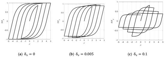
Figure 1. The influence of parameter δ_ν on strength degradation.

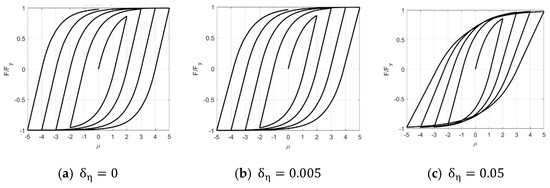
Figure 2. The influence of parameter δ_η on stiffness degradation.

Another nonlinear behavior, the pinching effect, is defined using function h as:

$$h\left(\dot{x},z,\epsilon \right)=1-{\zeta }_1{e}^{-{\left[z\cdot \mathrm{sign}(\dot{x})-q{z}_{\max }\right]}^2/{\zeta }_2^2}$$

(6)

$$z_{\max }={\left[\nu \left(\beta +\gamma \right)\right]}^{-1/n}$$

(7)

$${\zeta }_1\left(\epsilon \right)={\zeta }_s\left[1-e^{\left(-p\epsilon \right)}\right]$$

(8)

$${\zeta }_2\left(\epsilon \right)=\left(\psi +{\delta }_{\psi }\epsilon \right)\left(\lambda +{\zeta }_1\right)$$

(9)

where p, q, ζ_s, λ, ψ, and δ_ψ are all the parameters determining the pinching effect, which are explained in detail in the literature [28]. Specifically, ζ₁ sets the pinching severity, and ζ₂ sets the region where the pinching will spread. The influences of the key parameters ζ_s and λ are shown in Figure 3 and Figure 4. The decrease in loading and unloading stiffness in a certain region above and below the x-axis results in the whole cure pinching inward in the middle, which is the so-called pinching effect. The pinching phenomenon becomes more obvious as ζ_s increases. When λ equals 0.5, 1.0, or 2.0, the pinching region in the y-axis is [−0.3, 0.3], [−0.4, 0.4], or [−0.6, 0.6], respectively, indicating that the pinching scope increases as λ increases.

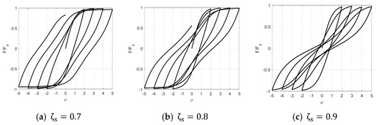
Figure 3. The influence of parameter ζ_s on pinching shape.

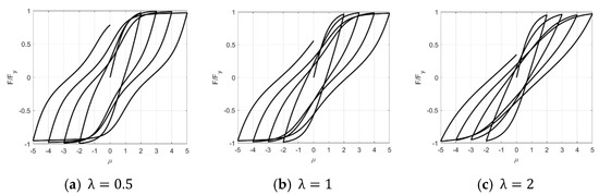
Figure 4. The influence of parameter λ on pinching shape.

2.2. Quasi-Static Experiment of RC HOLLOW Columns

Fourteen rectangular RC hollow columns, including seven square hollow columns, were tested under low-cycle reversed loading. The geometry of the cross-section is shown in Figure 5. The exterior dimensions were 800 mm × 500 mm (500 mm × 500 mm), and the web thickness was 120 mm. The design parameters are summarized in Table 1. The control variables included the section shape (rectangular and square), aspect ratio (h/b₁ = 4–8), longitudinal rebar ratio (ρ₀ = 1.63–2.69%), and volumetric stirrup ratio (ρ_v = 1.26–3.04%). All specimens were casted in C40 concrete (f_c = 40 MPa) with HRB 400 longitudinal rebar (f_y = 400 MPa) and HRB335 stirrup (f_ys = 335 MPa). According to engineering practice, the axial load ratios η_a of hollow bridge columns are usually approximately 5%; thus, all the specimens were loaded with a constant axial compression ratio of 5%. A schematic diagram of the loading system is shown in Figure 6. Vertical compression was applied using a jack with a spherical hinge and roller shaft to ensure the rotation and translation of the column tip. Horizontal lateral reversed loading was applied using an MTS hydraulic actuator.

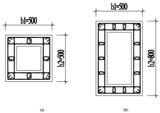
Figure 5. The geometry of the cross-section (units: mm). (a) Square hollow section, (b) Rectangular hollow section.

Table 1. Specimen design parameters for the quasi-static experiment.

ID	Depth b1/mm	Width b2/mm	Web Thickness d/mm	Column Height h/mm	Longitudinal Rebar Ratio ρ0/%	Stirrup Ratio ρv/%
D-1	500	500	120	1950	2.12	1.83
D-2	500	500	120	2950	2.12	1.83
D-3	500	500	120	3950	2.12	1.83
E-1	500	500	120	2950	2.12	2.51
E-2	500	500	120	2950	2.12	1.26
F-1	500	500	120	2950	1.87	1.83
F-2	500	500	120	2950	2.37	1.83
G-1	500	800	120	1950	2.15	2.13
G-2	500	800	120	2950	2.15	2.13
G-3	500	800	120	3950	2.15	2.13
H-1	500	800	120	2950	2.15	3.04
H-2	500	800	120	2950	2.15	1.42
I-1	500	800	120	2950	1.63	2.13
I-2	500	800	120	2950	2.69	2.13

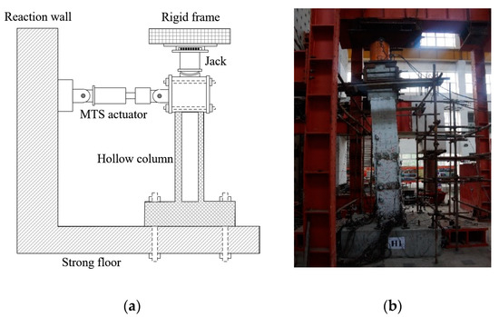
Figure 6. The schematic diagram of the loading system. (a) Schematic diagram of loading system, (b) Loading scene.

The force-displacement hybrid loading protocol was used as per the Specification for Seismic Test of Buildings [34]. Before the yielding of the specimen, the force-control mode was used. The yielding displacement was determined by sectional fiber analysis. The force applied at the column tip was repeated once in each level, that is, a certain proportion of the lateral load V_y = M_y/h (M_y is moment corresponding to the yielding displacement and h is the column height). The displacement-control mode was used after the yielding of specimen—namely, the column was put through displacement cycles twice at each loading level, as per the recommendation of ACI 374.2R-13 [35]. The amplitudes of displacement runs were the integral multiples of nominal yield displacement. The test was terminated when the lateral loading capacity dropped to 85% of the previous maximum force [34]. More design details, phenomena, and data analysis concerning the experiment can be found in the previous publication [33]. In this study, we focused on the hysteretic behaviors of hollow columns.

As revealed in the literature, due to the expansion of concrete cracks, along with the gradual crushing of kernel concrete in the compression area, the hollow column stiffness will decrease more severely with damage accumulation [36]. The stiffness characteristics during the unloading process directly determine the remaining performance. For example, residual displacement is the main factor controlling its repairable performance. Thus, the establishment of a hysteretic model that can accurately reflect the degradation of column stiffness would have significance, due also to the interest devoted to the maximum response before. Herein, the stiffness degradation index λ_s can be written as:

$${\lambda }_s=\frac{K_s^{+}/K_{sy}^{+}+K_s^{-}/K_{sy}^{-}}{2}$$

(10)

where $K_{\mathrm{s}}^{+}$ and $K_{\mathrm{s}}^{-}$ are the secant stiffness of the positive and negative loading directions in the loading cycle, respectively, and $K_{\mathrm{sy}}^{+}$ and $K_{\mathrm{sy}}^{-}$ are the corresponding secant stiffness levels at the equivalent yield points, respectively. The stiffness degradation index λ_s of each specimen measured in the quasi-static test above is shown in Figure 7. The peak displacement ductility coefficient μ_Max is defined as the ratio of the maximum inelastic displacement at each loading level to the equivalent yield displacement. As observed, there is a significant correlation between the stiffness degradation index of the column and its peak ductility coefficient. When the RC member reaches a new peak displacement, its overall stiffness decreases significantly.

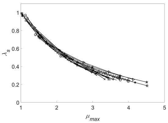
Figure 7. Stiffness degradation index λ_s.

2.3. The Improved BWBN Hysteretic Model

Given that the stiffness degradation index of an RC hollow column is roughly an exponential function with the ductility coefficient μ_Max, an exponential function with the peak displacement influencing factor r and ductility μ_Max is introduced to the stiffness degradation parameter η.

$$\eta =(1+{\delta }_{\eta }\epsilon )e^{r{\mu }_{\max }}$$

(11)

For intuitive comparison, the parameters in both BWBN models for RC members are taken as $\left[{\omega }_0, \alpha , \beta ,\gamma ,n,{\delta }_{\eta },{\delta }_{\nu },p,q, {\zeta }_{\mathrm{s}},\lambda ,\psi ,{\delta }_{\psi }\right]=$ $\left[1, 0.05, 0.5, 0.5, 2, 0.005, 0.05, 2.5, 0.15, 0.85, 1.5, 0.1, 0.005\right]$ as per the suggestion by Goda et al. [6]. For r = 0.05, the hysteretic curves of the original BWBN model and the improved BWBN model are shown in Figure 8. The y-axis is the ratio of restoring force F to yield force F_y, and the x-axis is the displacement ductility factor. By observing the slope change of the loading and unloading curves, it can be seen that the loading and unloading stiffness of the improved BWBN model decreases significantly as peak ductility increases, even outside the pinching region. This phenomenon clearly reveals that the degradation degree of member stiffness gradually intensifies with increasing lateral displacement. Furthermore, the unloading stiffness decreases significantly after reaching the new peak displacement. Thus, the unloading residual displacement can be adjusted accordingly by changing the r value.

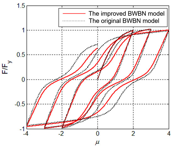
Figure 8. Comparison between improved and original BWBN model.

The influence of the peak displacement coefficient r (0.05, 0.10, and 0.15) on the shape of the hysteretic loops is shown in Figure 9. As observed, a larger r implies more obvious degradation of unloading stiffness as peak displacement increases and less residual displacement after unloading.

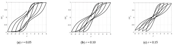
Figure 9. The influence of parameter r on the hysteretic shape.

To capture the inelastic restoring force of the improved BWBN hysteretic model, the hysteretic displacement z should be solved first. Note that z is given in the form of an implicit ordinary differential equation, so the fourth-order Runge–Kutta method was adopted because of calculation accuracy and efficiency.

3. Parameter Sensitivity Analysis of the Improved BWBN Model

Sensitivity analysis is a method to quantitatively describe the importance of input variables to output variables. In the improved BWBN hysteretic model, there are 13 undetermined parameters, including 4 shape parameters (α, β, γ, n), 3 degradation parameters (δ_η, r, δ_ν), and 6 pinch parameters (p, q, ζ_s, λ, ψ, δ_ψ). Changing each parameter within a reasonable range and studying and predicting the impact of each change on the hysteretic model is the so-called parameter sensitivity analysis of the hysteretic model. The sensitivity coefficient was used to quantitatively characterize the influences of the abovementioned parameters. The main purpose of parameter sensitivity analysis is to obtain the sensitivity coefficient ranking of these parameters and thereby screen out the core parameters of the hysteretic model to put further focus on the follow-up research. The scope of sensitivity analysis can be local or global. Local sensitivity analysis can only separately evaluate the impact of a single variable in the model, whereas global sensitivity analysis can consider the coupling between variables for comprehensive evaluation, and it is also known as importance analysis.

3.1. Local Sensitivity Analysis

3.1.1. The Procedure of Local Sensitivity Analysis

Local sensitivity analysis independently evaluates each parameter of the hysteretic model, which has strong operability due to convenience and simplicity. In this method, only one parameter is changed at a time, whereas other parameters are fixed as basic values. The sensitivity coefficient is constructed to evaluate the influences of parameter changes on the characteristics of the hysteretic model. The main purpose of the improved BWBN hysteretic model is to simulate the inelastic mechanical behavior of a structure during nonlinear dynamic time history analysis (NDTHA). Therefore, its sensitivity is defined by the influences of parameter changes on the results of NDTHA. The specific steps are presented next.

• According to the typical hysteretic characteristics of the object, the appropriate basic parameters were selected and taken into the hysteretic model for NDTHA. Based on the work by Ma et al. [37], the basic parameters in the improved BWBN model were $\left[\alpha ,\beta ,\gamma ,n\right]=\left[0.05, 0.5, 0.5, 2\right]$, $\left[{\delta }_{\eta },r,{\delta }_{\nu }\right]=\left[0.005, 0.1, 0.05\right]$, and $\left[p,q,{\zeta }_s,\lambda ,\psi ,{\delta }_{\psi }\right]=\left[2.5, 0.15, 0.85, 1.5, 0.1, 0.005\right]$, as shown in Figure 10.
  

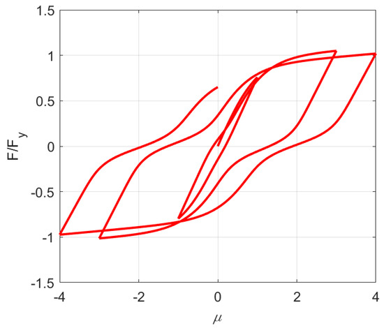  Figure 10. Shape diagram of the basic hysteretic curve.
• We changed only one parameter and kept the other parameters unchanged, followed by NDTHA again. Each parameter was changed by multiplying the current value by (1 + S_r), where S_r is a member of the set −50%, −30%, −20%, −10%, 10%, 20%, 30%, and 50%.
• We took all displacement responses obtained from NDTHA as the evaluation object. The displacement error function E_u can be defined as:

$$E_u{}_i=\frac{1}{t_m}\sqrt{{{\displaystyle \sum }}_{t=1}^{t_m}{\left[u_i\left(t\right)-u_0\left(t\right)\right]}^2}$$

(12)

where i is the parameter ID of the hysteretic model, 1–13; t is the time point of ground motion; t_m is the total number of time points; u₀ (t) is the displacement response at time t calculated by the basic model; and u_i (t) is the corresponding response after changing parameter i at time t. Each parameter will change 8 times, and the maximum error function calculated at each change is defined as the sensitivity coefficient of the parameter. The above process is repeated for each parameter in turn—that is, the sensitivity coefficients of each parameter can be obtained.

The excitation for local sensitivity analysis should possess a rich spectrum [37], so ground motions from actual seismic events are more suitable than artificial synthetic waves due to rich frequency characteristics. According to the investigation of highway bridge damage by the Wenchuan earthquake (M_w = 8.0) in China [38], the majority of damaged bridges are located in Type II sites according to the Chinese seismic code of highway bridges [39]. Thus, five earthquake records with V_s30 (average shear wave velocity in the top 30 m [40]) corresponding to Type II sites (260 < V_s30 < 510 m/s) were chosen from the NGA-West2 database as the input excitations. The information about records is listed in Table 2. The time history curves were scaled to a moderate PGA of 0.5 g (see Figure 11), which ensured the occurrence of strength and stiffness degradation and the pinching effect in RC hollow columns within a reasonable displacement ductility range [33]. The frequency spectrum of each scaled ground motion is shown in Figure 12. The Fourier spectra of these motions are different and consist of rich frequencies. Therefore, the results of local sensitivity analysis induced from the selected records would be applicable for a large class of cyclic excitation [37]. In the nonlinear dynamic time history analysis, the damping ratio of the structure is 0.05 and the natural vibration period of the structure is 1 s.

Table 2. The details of selected ground motions.

No.	Year	Record Name	Moment Magnitude	Rupture Distance/Km	Vs30/(m/s)	PGA/g	Mechanism
E1	1980	RSN287_ITALY_A-BOV000	6.9	46.25	356.39	0.0464	Normal
E2	1989	RSN731_LOMAP_A10000	6.93	41.97	391.91	0.1029	Reverse oblique
E3	1992	RSN826_CAPEMEND_EUR000	7.01	40.23	337.46	0.1552	Reverse
E4	1995	RSN1107_KOBE_KAK000	6.9	22.5	312.0	0.2476	Strike slip
E5	1979	RSN4459_MONTENE.GRO_VEL000	7.1	104.24	389.54	0.2739	Reverse

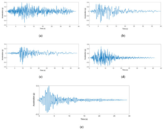
Figure 11. The time history curves of scaled ground motion records. (a) Ground motion E1, (b) Ground motion E2, (c) Ground motion E3, (d) Ground motion E4, (e) Ground motion E5.

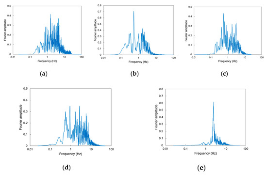
Figure 12. The frequency spectra of scaled ground motion records. (a) Ground motion E1, (b) Ground motion E2, (c) Ground motion E3, (d) Ground motion E4, (e) Ground motion E5.

3.1.2. The Results of Local Sensitivity Analysis

Five ground motion records were used for local sensitivity analysis, and the error function E_ui of each parameter is shown in Figure 13. When subjected to the same record, the ranking of E_ui at the same S_r indicates the sensitivity of the parameters to the improved BWBN model. The error function E_ui increases with increasing S_r, but the sensitivity ranking remains unchanged for most parameters. For the calculation results of different ground motion records, the sensitivity ranking of each parameter is slightly different, but the overall rankings are approximately the same.

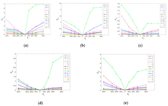
Figure 13. Error function corresponding to each ground motion. (a) Ground motion E1, (b) Ground motion E2, (c) Ground motion E3, (d) Ground motion E4, (e) Ground motion E5.

The maximum value of the error function calculated by eight S_r variation points is regarded as the sensitivity coefficient of the parameter. For a clear and detailed presentation, the tornado graphs of parameters, each corresponding to a ground motion dataset, are shown in Figure 14. It can be concluded that the parameter with the highest local sensitivity is ζ_s, which controls the degree of pinch. The rankings of parameters $\alpha$, $\beta$, $\gamma$, $n$, and $\psi$, which are the shape parameters in the original Bouc–Wen model [20,21], exhibit some discrepancies when excited with different records, yet they are consistently ranked highly, and they can be termed core parameters. The rankings of parameters r, δ_ν, q, and λ mainly controlling degradation and pinching are in the middle, and they can be termed important parameters in consideration of their explicit physical meanings. The sensitivity of the remaining parameters is low, and they can be taken as secondary parameters. For the massive computation of the improved BWBN model, it is often necessary to select parameters for analysis according to the research purpose.

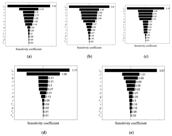
Figure 14. Tornado graph of hysteretic model parameters. (a) Ground motion E1, (b) Ground motion E2, (c) Ground motion E3, (d) Ground motion E4, (e) Ground motion E5.

3.2. Global Sensitivity Analysis

3.2.1. The Procedure of Global Sensitivity Analysis

The global sensitivity analysis can comprehensively consider the influence of the coupling effect on the final output in relation to multiple parameters, making it more refined than local sensitivity analysis (considering only one parameter). The main steps are outlined as follows.

• Define the target function as Y = f(X), which can be decomposed into the following form by ANOVA (analysis of variance):

$$f\left(X\right)=f_0+{\displaystyle \sum }_{s=1}^n{\displaystyle \sum }_{i_1<\dots <i_s}^{}{f}_{i_1\dots i_s}\left(x_{i_1},\dots ,x_{i_s}\right)$$

(13)

where X is an n-dimensional vector representing n input parameters, and each parameter obeys a [0, 1] uniform distribution.

2.

Sobol proposed a variance sensitivity analysis method that can consider the coupling between parameters based on the decomposed variance. The total variance of f(X) defined in this method is:

$$D=f^2\left(X\right)dX-f_0^2$$

(14)

The variance of each subitem is:

$$D_{i_1\dots i_s}={\displaystyle \int \dots }{\displaystyle \int f_{i_1\dots i_s}^2\left(x_{i_1},\dots ,x_{i_s}\right)d{x}_{i_1}\dots d{x}_{i_s}}$$

(15)

In particular, when the subitem contains only one input parameter, there are:

$$D_i={\displaystyle \int f_i^2\left(x_i\right)d{x}_i}$$

(16)

The Sobol method defines the first-order sensitivity $S_i$ coefficient of the ith parameter x_i as follows:

$$S_i=\frac{D_i}{D}$$

(17)

Coefficient $S_i$ reflects the influence of x_i alone on model output response f(X) in the form of variance change. That is, a larger $S_i$ means a greater influence of parameter x_i, which indicates that the system is more sensitive to this parameter. Similarly, the higher-order sensitivity coefficient ${\mathrm{S}}_{i_1\dots i_{\mathrm{s}}}$ representing the sensitivity under the combined action of parameters can be written as:

$$S_{i_1\dots i_s}=\frac{D_{i_1\dots i_s}}{D}$$

(18)

The overall sensitivity coefficient $S_i^{Tol}$ is defined as the sum of sensitivity coefficients with regard to x_i.

$$S_i^{Tol}=S_i+{\displaystyle \sum }_{i\ne j}{S}_{ij}+\dots +S_{1,2\dots ,i\dots ,n}=1-\frac{D_{~i}}{D}$$

(19)

where $D_{–i}$ is the sum of the variances of the subitems excluding that of x_i, which can be obtained by subtracting $D_{–i}$ from the total variance D.

The Sobol method not only reflects the sensitivity of parameter x_i but also better reflects the sensitivity of this parameter and other parameters under all coupling conditions. Obviously, X = {x₁, x₂... x₁₃} are the 13 undetermined parameters in the improved BWBN hysteretic model, and Y is the target variable after NDTHA using a set of model parameters. As per the literature [5,6,7,8,9], the peak displacement and residual displacement are taken as the target variables.

3.

The Monte Carlo method is used to estimate the variance of the model output and thereby complete the aforementioned global sensitivity analysis procedure.

3.2.2. The Results of Global Sensitivity Analysis

The ground motion records used in NDTHA to obtain the target variables for the global sensitivity analysis were the same as those used in the local sensitivity analysis. The overall sensitivity coefficients $S_i^{Tol}$ corresponding to the peak displacement and residual displacement are shown in Table 3 and Table 4, respectively. For the peak displacement, the rankings of the overall sensitivity coefficients $S_i^{Tol}$ under different ground motions are almost the same, indicating that the influence of input excitations is insignificant. The parameters of $\alpha$, $\beta$, and $\gamma$ in the original Bouc–Wen model [20,21] and the parameter ${\zeta }_{\mathrm{s}}$ controlling the pinching rank first, so they are the core parameters. The parameters $n$, $\psi$, $r$, $q, \mathrm{and} \lambda$ are taken as important parameters, and the remaining parameters are defined as secondary parameters. In regard to the residual displacement, r, regarded as a core parameter, ascends from 5–8 to 2–3. As a result, the improved BWBN utilizing r is reasonable, since the peak and residual performance are both given great attention in the repairable-based seismic design.

Table 3. Global sensitivity $S_i^{Tol}$ coefficients of peak displacement.

Parameter	E1		E2		E3		E4		E5
	${\mathit{S}}_{\mathit{i}}^{\mathit{T}\mathit{o}\mathit{l}}$	Rank	${\mathit{S}}_{\mathit{i}}^{\mathit{T}\mathit{o}\mathit{l}}$	Rank	${\mathit{S}}_{\mathit{i}}^{\mathit{T}\mathit{o}\mathit{l}}$	Rank	${\mathit{S}}_{\mathit{i}}^{\mathit{T}\mathit{o}\mathit{l}}$	Rank	${\mathit{S}}_{\mathit{i}}^{\mathit{T}\mathit{o}\mathit{l}}$	Rank
$\alpha$	0.0435	3	0.0985	3	0.1410	3	0.1325	4	0.1126	3
$\beta$	0.3916	1	0.4433	1	0.4081	1	0.2700	1	0.4373	1
$\gamma$	0.2474	2	0.2561	2	0.2061	2	0.1811	2	0.2869	2
$n$	0.0079	7	0.0106	7	0.0159	5	0.0123	7	0.0104	7
${\delta }_{\eta }$	0.0003	12	0.0007	11	0.0009	11	0.0016	11	0.0009	10
${\delta }_{\nu }$	0.0040	9	0.0053	8	0.0010	10	0.0068	10	0.0007	11
$r$	0.0266	6	0.0187	5	0.0015	8	0.0341	5	0.0417	5
${\zeta }_{\mathrm{s}}$	0.0267	5	0.0363	4	0.0199	4	0.1349	3	0.0421	4
$q$	0.0022	10	0.0003	12	0.0003	13	0.0071	8	0.0012	9
$\psi$	0.0328	4	0.0111	6	0.0081	6	0.0253	6	0.0231	6
$\lambda$	0.0076	8	0.0028	9	0.0030	7	0.0068	9	0.0075	8
$p$	0.0001	13	0.0002	13	0.0003	12	0.0001	13	0.0000	13
${\delta }_{\psi }$	0.0004	11	0.0009	10	0.0013	9	0.0003	12	0.0001	12

Table 4. Global sensitivity $S_i^{Tol}$ coefficients of residual displacement.

Parameter	E1		E2		E3		E4		E5
	${\mathit{S}}_{\mathit{i}}^{\mathit{T}\mathit{o}\mathit{l}}$	Rank	${\mathit{S}}_{\mathit{i}}^{\mathit{T}\mathit{o}\mathit{l}}$	Rank	${\mathit{S}}_{\mathit{i}}^{\mathit{T}\mathit{o}\mathit{l}}$	Rank	${\mathit{S}}_{\mathit{i}}^{\mathit{T}\mathit{o}\mathit{l}}$	Rank	${\mathit{S}}_{\mathit{i}}^{\mathit{T}\mathit{o}\mathit{l}}$	Rank
$\alpha$	0.4422	1	0.7859	1	0.3592	4	0.4828	3	0.4193	3
$\beta$	0.3739	3	0.5855	3	0.5483	1	0.5305	1	0.8060	1
$\gamma$	0.3666	4	0.4447	5	0.4516	2	0.4803	4	0.3157	5
$n$	0.0971	8	0.1519	9	0.2118	6	0.1534	6	0.0962	7
${\delta }_{\eta }$	0.0027	12	0.0857	10	0.0183	11	0.0523	10	0.0015	13
${\delta }_{\nu }$	0.0284	10	0.0007	13	0.0492	10	0.0259	11	0.0133	11
$r$	0.3771	2	0.7555	2	0.3773	3	0.5259	2	0.4902	2
${\zeta }_{\mathrm{s}}$	0.3198	5	0.4886	4	0.2400	5	0.4648	5	0.3607	4
$q$	0.1357	7	0.3521	6	0.1339	8	0.1481	7	0.1006	6
$\psi$	0.1845	6	0.2787	8	0.1684	7	0.1373	8	0.0905	9
$\lambda$	0.0518	9	0.3072	7	0.0961	9	0.1017	9	0.0949	8
$p$	0.0017	13	0.0031	12	0.0014	13	0.0019	13	0.0016	12
${\delta }_{\psi }$	0.0218	11	0.0387	11	0.0177	12	0.0238	12	0.0207	10

Although the importance of parameters in the improved BWBN hysteretic model was clarified using the local and global-level methods, the hysteretic curves of hollow columns are the specific combinations of these parameters. Note that there are a total of thirteen parameters in the improved BWBN model, and the PSOGSA algorithm [41] was implemented in this study for identification based on quasi-static tests.

4. Parameter Identification for the RC Hollow Columns

4.1. Review of PSOGSA Algorithm

The hybrid population-based algorithm (PSOGSA) is a combination of particle swarm optimization (PSO) and the gravitational search algorithm (GSA) [41]. To combine these algorithms, Equation (20) is used as follows:

$$V_i(t+1)=w\times V_i(t)+{c^{\prime }}_1\times rand\times a_i(t)+{c^{\prime }}_2\times rand\times [gbest-X_i(t)]$$

(20)

$$X_i(t+1)=X_i(t)+V_i\left(t+1\right)$$

(21)

where X_i(t) and V_i(t) are the position and velocity of agent i at iteration t; w is a weighting function; $c_1^{\prime }$ and $c_2^{\prime }$ are the weighting factors; rand is a random number between 0 and 1; and gbest is the best solution thus far. In each iteration, the positions of the particles are updated as in Equation (21). a_i(t) is the acceleration of agent i at iteration t, which can be calculated as:

$$a_i(t)=\frac{F_i(t)}{M_i(t)}$$

(22)

$$F_i(t)={\displaystyle {\sum }_{j=1,j\ne i}^{N}ran{d}_j{F}_{ij}^d(t)}$$

(23)

where t is a specific time; M_i(t) is the mass of object i; F_i(t) is the total force that acts on agent i in a problem space with dimensions d. The gravitational forces from agent j on agent i at a specific time t are defined as:

$$F_{ij}^d(t)=G(t)\frac{M_{pi}(t)M_{aj}(t)}{R_{ij}+{\epsilon }_{\mathrm{con}}}[X_i(t)-X_j(t)]$$

(24)

where M_pi(t) and M_aj(t) are the passive and active gravitational mass related to agent i and agent j, respectively; G(t) is a gravitational constant at time t; ε_con is a small constant; and R_ij is the Euclidian distance between two agents i and j. In each iteration, the best solution thus far should be updated. After calculating the accelerations and updating the best solution thus far, the velocities of all agents can be calculated using Equation (20). Finally, the positions of agents are defined as Equation (21). The process of updating velocities and positions will be stopped by meeting an end criterion.

In the process of parameter identification using the PSOGSA algorithm, a set of parameter vectors Φ is defined, which produced the 14 parameters in the improved BWBN model. The goal of parameter identification is to find the optimal parameter Φ that produces the smallest error between the restoring force of the predicted hysteretic model and measured loops. Here, the function E, for quantitatively describing the error, is defined as follows:

$$E=\frac{1}{\max [F_e(t)]}\sqrt{\frac{1}{N}{\displaystyle {\sum }_{t=1}^N{[F_e(t)-F_m(t)]}^2}}$$

(25)

where t is the loading step; F_e(t) and F_m(t) are the measured restoring force and simulated restoring force at each step, respectively; and N is the total loading steps. The error function contains all the measured data points of the hysteretic curve. Each identification needs to analyze the simulation accuracy of all data points in the whole loading process to ensure the accuracy of the final identification.

4.2. Identification of the Hysteretic Model

Since the axial load is the significant parameter influencing the shape of a hysteretic curve, two specimens by Mander et al. [42] were added as members of the hollow column database. The design parameters of the two supplied columns are listed in Table 5, the main distinction being axial values of 0.1 and 0.3. To ensure the generality of the parameter identification, the measured hysteretic curve was normalized by the yield displacement and yield force in the x-axis and y-axis, respectively. The identified parameters of the improved BWBN model for these sixteen hollow specimens are presented in Table 6, along with the range of each parameter, as shown in Table 7. The predicted and experimental hysteretic curves of sixteen hollow columns are shown in Figure 15. As seen, the hysteretic model with the parameters identified by PSOGSA can fully describe the restoring force characteristics of the specimen. The phenomena of strength and stiffness degradation and the pinching effect are clearly displayed. Furthermore, the fitness function set in the parameter identification process contains all the data for the whole loading process. The loading history of the tested and identified restoring forces of six hollow columns with different aspect ratios are shown in Figure 16. It is clear that the loading steps of the improved BWBN hysteretic model almost coincide with the measured data.

Table 5. Design parameters of specimens by Mander et al. [42].

ID	b1/mm	b2/mm	d/mm	h/mm	ηa	${\rho }_0$/%	${\rho }_v$/%	$f_y$/MPa	$f_c$/MPa
M-A	750	750	120	3250	0.1	1.55	0.74	335	30
M-C	750	750	120	3250	0.3	1.55	0.83	335	29

Table 6. Identified parameters of the improved BWBN hysteretic model for hollow columns.

ID	$\mathit{\alpha }$	$\mathit{\beta }$	$\mathit{\gamma }$	$\mathit{n}$	${\mathit{\delta }}_{\mathit{\eta }}$	${\mathit{\delta }}_{\mathit{\nu }}$	$\mathit{r}$	${\mathit{\zeta }}_{\mathit{s}}$	$\mathit{p}$	$\mathit{q}$	$\mathit{\psi }$	${\mathit{\delta }}_{\mathit{\psi }}$	$\mathit{\lambda }$
D-1	0.07	0.75	−0.06	1.15	1.04 × 10−5	0.08	0.06	0.63	0.46	0.05	0.57	1.58 × 10−4	1.73
D-2	0.02	0.95	−0.35	0.84	1.08 × 10−4	0.07	0.03	0.72	0.20	0.05	0.58	1.61 × 10−4	2.57
D-3	0.02	1.36	−0.50	0.94	1.00 × 10−5	0.11	0.11	0.69	0.91	0.05	0.33	1.54 × 10−4	4.68
E-1	0.06	1.34	−0.26	1.74	1.00 × 10−5	0.11	0.05	0.61	0.71	0.09	0.37	1.54 × 10−4	3.91
E-2	0.04	0.80	−0.01	0.91	1.00 × 10−5	0.05	0.08	0.66	0.63	0.08	0.56	1.56 × 10−4	1.99
F-1	0.04	1.13	−0.50	1.22	5.51 × 10−5	0.07	0.09	0.64	0.50	0.18	0.40	1.51 × 10−4	4.60
F-2	0.04	1.21	−0.49	1.73	1.00 × 10−5	0.09	0.10	0.59	0.75	0.14	0.31	1.57 × 10−4	2.80
G-1	0.02	0.71	−0.40	0.88	1.00 × 10−5	0.08	0.17	0.63	0.59	0.07	0.54	1.50 × 10−4	3.39
G-2	0.04	0.54	−0.12	1.25	2.13 × 10−4	0.09	0.06	0.64	0.50	0.17	0.44	1.23 × 10−4	1.61
G-3	0.03	1.26	−0.46	1.14	1.09 × 10−5	0.11	0.12	0.66	1.02	0.28	0.35	1.48 × 10−4	3.80
H-1	0.02	0.59	−0.28	1.50	1.00 × 10−5	0.30	0.15	0.60	0.64	0.18	0.27	1.78 × 10−4	3.64
H-2	0.02	0.70	−0.34	0.89	2.47 × 10−4	0.15	0.20	0.58	0.62	0.06	0.53	1.48 × 10−4	4.37
I-1	0.03	0.90	−0.50	0.93	4.92 × 10−5	0.06	0.15	0.61	0.41	0.06	0.62	1.74 × 10−4	2.76
I-2	0.04	0.85	−0.16	1.24	1.00 × 10−5	0.09	0.06	0.69	0.47	0.05	0.51	1.42 × 10−4	1.83
M-A	0.05	1.38	−0.34	1.47	4.75 × 10−5	0.12	0.05	0.72	1.03	0.17	0.41	1.15 × 10−4	2.70
M-C	0.02	0.70	−0.17	2.12	1.09 × 10−4	0.12	0.12	0.67	0.56	0.05	0.70	1.97 × 10−4	1.59

Table 7. Reasonable ranges of hysteretic parameters for hollow columns.

Parameters	$\mathit{\alpha }$	$\mathit{\beta }$	$\mathit{\gamma }$	$\mathit{n}$	${\mathit{\delta }}_{\mathit{\eta }}$	${\mathit{\delta }}_{\mathit{\nu }}$	$\mathit{r}$	${\mathit{\zeta }}_{\mathit{s}}$	$\mathit{p}$	$\mathit{q}$	$\mathit{\psi }$	${\mathit{\delta }}_{\mathit{\psi }}$	$\mathit{\lambda }$
Lower bound	0.02	0.5	−0.5	0.8	1.00 × 10−5	0.05	0.05	0.55	0.2	0.05	0.3	1.50 × 10−4	1.5
Upper bound	0.07	1.5	0	2	2 × 10−4	0.2	0.2	0.8	1	0.2	0.7	2 × 10−4	4.6

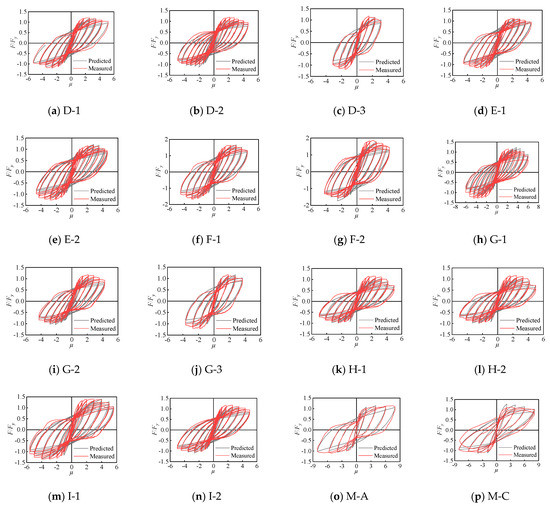
Figure 15. The predicted and measured hysteresis curves.

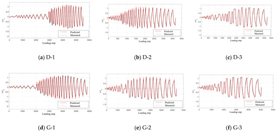
Figure 16. The predicted and measured loading step curves.

In mathematical statistics, the coefficient of determination R² is usually used to evaluate the fitting degree of the numerical model to the measured values:

$$R^2=1-\frac{{{\displaystyle \sum }}_{i=1}^n{\left(y_i-{\widehat{y}}_i\right)}^2}{{{\displaystyle \sum }}_{i=1}^n{\left(y_i-\overline{y_i}\right)}^2}$$

(26)

where $y_{\mathrm{i}}$ is the measured value, ${\widehat{y}}_i$ is the predicted value, and $\overline{y_i}$ is the average value of the measured data. The closer R² is to 1, the more accurate the numerical model. The coefficient of determination R² and error function E of the hysteretic curves predicted by the improved BWBN model, with regard to the measured ones, are shown in Table 8. The values of R² are all larger than 0.96, and E is less than 0.004, indicating that the BWBN model identified by PSOGSA matched all experimental loops with satisfactory and reasonable accuracy.

Table 8. R² and E for hollow column specimens.

ID	D-1	D-2	D-3	E-1	E-2	F-1	F-2	G-1	G-2	G-3	H-1	H-2	I-1	I-2	M-A	M-C	Mean
R2	0.9786	0.9763	0.9824	0.9878	0.9828	0.9791	0.9758	0.9677	0.9801	0.9821	0.9734	0.9831	0.9828	0.9862	0.9723	0.9742	0.9790
E	0.0007	0.0011	0.0009	0.0008	0.001	0.0009	0.0007	0.001	0.0008	0.001	0.0007	0.0007	0.0008	0.0007	0.0036	0.0029	0.0011

5. Prediction and Validation of the Improved BWBN Model

To simulate the hysteretic curve of elements with the improved BWBN hysteretic model, the important thing is obtaining the parameters accurately. For a hollow column whose hysteretic curve has been obtained by testing, the parameters can be directly acquired by an intelligent optimization algorithm. However, the hollow columns often lack tested hysteretic loops, and for these it is necessary to develop an effective empirical prediction method relating the improved BWBN model parameters and the design physical parameters of RC hollow columns.

5.1. Regression of Hysteretic Model Parameters

Obviously, the empirical prediction does not need to take into account all parameters. According to the previous local and global sensitivity analyses, ${\delta }_{\eta }$, $p$, and ${\delta }_{\psi }$ are the secondary parameters that have little influence on the hysteretic characteristics. Thus, they can be taken as constants, that is, ${\delta }_{\eta }=1\times {10}^{-5}$, $p=0.5$, and ${\delta }_{\psi }=1.5\times {10}^{-5}$, as listed in Table 7. The other ten parameters can be categorized into two groups. That is, parameters $\alpha$, $\beta$, $n$, ${\delta }_{\nu }$, $r$, ${\zeta }_{\mathrm{s}}$, $\lambda$, $\psi$, $q$, and $\lambda$ belong to P₁, and parameter r belongs to P₂. If the relationship of P₁ and P₂ and design parameters are given, the improved BWBN hysteretic model of hollow columns can be determined independent of quasi-static tests. As per the literature and experiments in this study, the primary design parameters of hollow columns include section depth b₁, section width b₂, web thickness d, column height h, axial load ratio η_a, longitudinal rebar ratio ${\rho }_0$, volumetric stirrup ratio ${\rho }_{\mathrm{v}}$, yield strength of longitudinal rebar $f_y$, and concrete compressive strength $f_c$. In regression analysis, dimensionless treatment of design parameters can ensure the universality of regression results. Thus, the design parameters with dimensions of length are normalized by the section depth b₁ along the loading direction, and the yield strength of longitudinal rebar f_y is normalized by the compressive strength of concrete f_c. The exponential functions are used to express the relationships between the design parameters and hysteretic model parameters, and are written as follows:

$$P_1=e^{x_1\times b_2/b_1+x_2\times d/b_1+x_3\times h/b_1+x_4\times \eta +x_5\times {\rho }_0+x_6\times {\rho }_{sv}+x_7\times f_y/f_c+x_8}$$

(27)

$$P_2=-e^{x_1\times b_2/b_1+x_2\times d/b_1+x_3\times h/b_1+x_4\times \eta +x_5\times {\rho }_0+x_6\times {\rho }_{sv}+x_7\times f_y/f_c+x_8}$$

(28)

where P₁ is associated with $\alpha$, $\beta$, $n$, ${\delta }_{\nu }$, $r$, ${\zeta }_s$, $\lambda$, $\psi$, $q$, and $\lambda$; and P₂ is only associated with r. x_i (i = 1–8) are the empirical coefficients, reflecting the importance of hysteretic model parameters influenced by pier design parameters. The greater the absolute value of the coefficient xi, the stronger the correlation between the corresponding design parameters and hysteretic model parameters. As the influences of the design parameters on the 10 parameters of the improved BWBN model are different, the eight empirical coefficients corresponding to each hysteretic model parameter need to be determined separately. Using the least square method for nonlinear regression analysis, the empirical coefficient xi for each hysteretic parameter can be obtained based on the identified parameters of the improved BWBN model in Table 6.

Based on Equations (27) and (28), and the regressed coefficients x_i in Table 9, the empirical prediction method can be summarized as follows.

Table 9. Empirical coefficient of parameters for the hollow column hysteretic model.

	${\mathit{x}}_1$	${\mathit{x}}_2$	${\mathit{x}}_3$	${\mathit{x}}_4$	${\mathit{x}}_5$	${\mathit{x}}_6$	${\mathit{x}}_7$	${\mathit{x}}_8$
$\alpha$	−0.993	−2.600	−0.172	−5.049	0.372	0.298	0.122	−2.473
$\beta$	−0.524	−5.445	0.169	−3.676	0.000	0.150	0.116	−0.051
$\gamma$	−0.310	−16.783	0.261	−2.943	−1.211	0.202	−0.265	5.768
$n$	−0.436	−5.623	0.003	1.451	0.412	0.424	0.090	−0.397
${\delta }_{\nu }$	0.194	19.570	0.086	−1.908	0.212	1.000	0.838	−16.067
$r$	1.151	0.725	−0.035	5.272	−0.519	−0.266	−0.304	−0.305
${\zeta }_s$	−0.043	1.485	0.018	−0.443	0.071	−0.016	0.071	−1.447
$q$	0.618	5.006	0.316	−7.662	−0.093	0.475	0.624	−10.946
$\psi$	0.245	−19.424	−0.114	4.005	−0.307	−0.340	−0.607	9.579
$\lambda$	−0.226	−3.248	0.150	−2.645	−0.423	0.160	−0.031	2.237

• Substitute the coefficients xi in Table 9 into Equations (27) and (28), and the prediction formulas of 10 parameters for BWBN model are obtained. For example,

$$\begin{array}{l}{\omega }_0=exp(-0.248\times b_2/b_1-0.268\times d/b_1+0.101\times h/b_1-0.678\times \eta -0.102\times {\rho }_0-0.093\times {\rho }_{sv}\\ +-0.058\times f_y/f_c+1.103)\end{array}$$

(29)

$$\begin{array}{l}\gamma =-\exp (-0.310\times b_2/b_1-16.783\times d/b_1+0.261\times h/b_1-2.943\times \eta -1.211\times {\rho }_0+0.202\times {\rho }_{sv}\\ -0.265\times f_y/f_c+5.768)\end{array}$$

(30)

2.

The design parameters of the hollow column are substituted into the prediction formulas to obtain each hysteretic parameter.

3.

Take the 10 parameters above, along with ${\delta }_{\eta }=1\times {10}^{-5}, p=0.5$, and ${\delta }_{\psi }=1.5\times {10}^{-5}$, into the improved BWBN model. Once the loading history is offered, the hysteretic curves of the hollow column can be predicted using such an empirical method.

5.2. Validation of the Empirical Prediction Method

To check the applicability of the empirical prediction method, the hollow column specimen by Zhang et al. [43] was selected. The design parameters of the selected member (ID = RC) are shown in Table 10. Taking these design parameters into the prediction equations (e.g., Equation (29) or Equation (30)), the predicted parameters needed for the improved BWBN hysteretic model are listed in Table 11. The predicted and measured hysteretic curves of selected RC hollow column are compared in Figure 17. It is obvious that the improved BWBN model with predicted parameters can well match the original test loops. The inelastic behavior, including strength and stiffness degradation, and the pinching phenomenon of the hollow column, can be well reproduced. The R² is 0.83 for the selected hollow specimen, and although slightly lower than that for method using the direct identification by PSOGSA, is still over 0.80, implying reasonable accuracy. Furthermore, a comparison of the predicted and measured residual displacements is shown in Figure 18. It is clear that the improved BWBN hysteretic model equipped with the empirical prediction method can offer accurate residual displacement in addition to the peak responses. In short, the overall and residual hysteretic behaviors of the RC hollow columns can be obtained quickly if the parameters of the improved BWBN model are given by an empirical method.

Table 10. Design parameters of the selected hollow column.

ID	b1/mm	b2/mm	d/mm	h/mm	η	${\mathit{\rho }}_0/\%$	${\mathit{\rho }}_{\mathit{v}}/\%$	${\mathit{f}}_{\mathit{y}}/\mathbf{MPa}$	${\mathit{f}}_{\mathit{c}}/\mathbf{MPa}$
RC	360	360	100	1600	0.1	1.4	0.72	335	38.7

Table 11. Predicted parameters of the selected hollow column.

ID	ω0	α	β	γ	n	δη	δν	r	ζs	p	q	Ψ	δψ
RC	1.25	0.03	0.55	−0.11	0.56	1.18 × 10−4	0.14	0.12	0.71	0.34	0.07	0.2	2.15

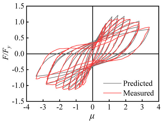
Figure 17. The predicted and measured hysteresis curves.

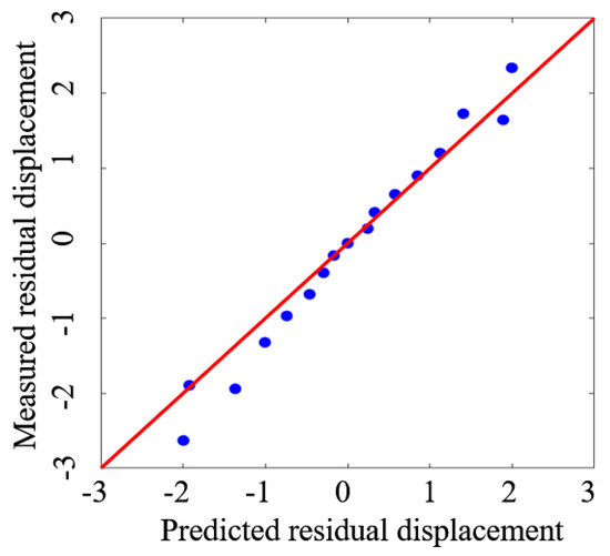
Figure 18. The predicted and measured residual displacement.

6. Conclusions

In this study, an improved symmetrical BWBN hysteretic model was proposed, and sensitivity analysis was performed. The improved BWBN parameters were further identified and calibrated based on a set of 16 hollow columns. Based on the work implemented, the main conclusions are as follows:

(1)

The coefficient r introduced to the original BWBN model can reflect the correlation between column stiffness degradation and maximum displacement. r can directly control the residual displacement of the hysteretic model; thus, the accuracy of residual displacement can be improved apart from the existing inelastic behavior, via factors such as strength and stiffness degradation, and a pinching effect.

(2)

In the improved BWBN model, $\alpha$, $\beta$, $\gamma$, and ${\zeta }_{\mathrm{s}}$ are the core parameters according to both local and global sensitivity analyses; $n$, $\psi$, $r$, $q$, and $\lambda$ are at least important according to local or global sensitivity analysis; and $p$, ${\delta }_{\eta }$, and ${\delta }_{\psi }$ are the parameters that have little influence. In particular, r can be taken as a core parameter if focused on the residual displacement.

(3)

The hybrid intelligence algorithm PSOGSA can accurately identify the parameters of the improved BWBN hysteretic model for the rectangular hollow column, which is an efficient and powerful tool for such parameter identification of hysteretic models of other RC members.

(4)

Empirical prediction equations were regressed to build the relationship between the BWBN model and design parameters of hollow columns, which can be an efficient and convenient way to obtain hysteretic curves for members without experimental loops. Although the accuracy of the predicted hysteretic loops was slightly lower than that of the directly calibrated loops, it was still sufficient for engineering practice.

(5)

Widespread applicability of empirical equations predicting the parameters of the improved BWBN model for the hollow columns should be validated by more experimental tests in the future research.

References

- Kawashima, K.; Unjoh, S. The damage of highway bridges in the 1995 hyogo-ken nanbu earthquake and its impact on Japanese seismic design. J. Earthq. Eng. 1997, 3, 505–541. [Google Scholar] [CrossRef]
- Sun, Z.; Wang, D.; Guo, X.; Si, B.; Huo, Y. Lessons Learned from the Damaged Huilan Interchange in the 2008 Wenchuan Earthquake. J. Bridg. Eng. 2012, 17, 15–24. [Google Scholar] [CrossRef]
- Ma, F.; Ng, C.H.; Ajavakom, N. On system identification and response prediction of degrading structures. Struct. Control Health Monit. 2005, 13, 347–364. [Google Scholar] [CrossRef]
- Zhang, Y.; Han, S. Hysteretic Model for Flexure-shear Critical Reinforced Concrete Columns. J. Earthq. Eng. 2018, 22, 1639–1661. [Google Scholar] [CrossRef]
- Ruiz-García, J.; Miranda, E. Probabilistic estimation of residual drift demands for seismic assessment of multi-story framed buildings. Eng. Struct. 2010, 32, 11–20. [Google Scholar] [CrossRef]
- Goda, K.; Hong, H.P.; Lee, C.S. Probabilistic Characteristics of Seismic Ductility Demand of SDOF Systems with Bouc-Wen Hysteretic Behavior. J. Earthq. Eng. 2009, 13, 600–622. [Google Scholar] [CrossRef]
- Iervolino, I.; Chioccarelli, E.; Baltzopoulos, G. Inelastic displacement ratio of near-source pulse-like ground motions. Earthq. Eng. Struct. Dyn. 2012, 41, 2351–2357. [Google Scholar] [CrossRef]
- Ning, C.; Cheng, Y.; Yu, X.-H. A Simplified Approach to Investigate the Seismic Ductility Demand of Shear-Critical Reinforced Concrete Columns Based on Experimental Calibration. J. Earthq. Eng. 2019, 25, 1958–1980. [Google Scholar] [CrossRef]
- Ruiz-Garcia, J. On the influence of strong-ground motion duration on residual displacement demands. Earthquakes Struct. 2010, 1, 327–344. [Google Scholar] [CrossRef]
- Sivaselvan, M.V.; Reinhorn, A.M. Hysteretic Models for Deteriorating Inelastic Structures. J. Eng. Mech. 2000, 126, 633–640. [Google Scholar] [CrossRef]
- Veletsos, A.S.; Newmark, N.M.; Chelapati, C.V. Deformation spectra for elastic and elastoplastic systems subjected to ground shock and earthquake motions. In Proceedings of the 3rd World Conference on Earthquake Engineering, Auckland/Wellington, New Zealand, 22 January–1 February 1965; pp. 663–682. [Google Scholar]
- Clough, R.W.; Johnston, S.B. Effect of stiffness degradation on earthquake ductility requirements. In Proceedings of the Second Japan National Conference on Earthquake Engineering Symposium, Tokyo, Japan; 1966; pp. 227–232. Available online: http://library.jsce.or.jp/Image_DB/eq1994/proc/ab/id44006.html (accessed on 1 January 2022).
- Takeda, T.; Sozen, M.A.; Nielsen, N.N. Reinforced Concrete Response to Simulated Earthquakes. J. Struct. Div. 1970, 96, 2557–2573. [Google Scholar] [CrossRef]
- Saidi, M.; Sozen, M.A. Simple and complex models for nonlinear seismic response of reinforced concrete structures. In A Report to the National Science Foundation; University of Illinois at Urbana-Champaign: Urbana, IL, USA, 1979. [Google Scholar]
- Ozcebe, G.; Saatcioglu, M. Hysteretic Shear Model for Reinforced Concrete Members. J. Struct. Eng. 1989, 115, 132–148. [Google Scholar] [CrossRef]
- Dowell, R.K.; Seible, F.; Wilson, E.L. Pivot hysteresis model for reinforced concrete members. ACI Struct. J. 1998, 95, 607–617. [Google Scholar]
- Sucuoglu, H.; Erberik, A. Energy based hysteresis and damage models for deteriorating systems. Earthq. Eng. Struct. Dyn. 2004, 33, 69–88. [Google Scholar] [CrossRef]
- Ibarra, L.F.; Medina, R.A.; Krawinkler, H. Hysteretic models that incorporate strength and stiffness deterioration. Earthq. Eng. Struct. Dyn. 2005, 34, 1489–1511. [Google Scholar] [CrossRef]
- Li, J.Z.; Guan, Z.G. Research progress on bridge seismic design: Target from seismic alleviation to post-earthquake structural resilience. China J. Highw. Transp. 2017, 30, 1–9, 59. (In Chinese) [Google Scholar]
- Bouc, R. Forced vibration of mechanical systems with hysteresis. In Proceedings of the Fourth Conference on Nonlinear Oscillation, Prague, Czechoslovakia, 5–9 September 1967; pp. 315–318. [Google Scholar]
- Wen, Y.-K. Method for Random Vibration of Hysteretic Systems. J. Eng. Mech. Div. 1976, 102, 249–263. [Google Scholar] [CrossRef]
- Baber, T.T.; Wen, Y.-K. Random Vibration of Hysteretic, Degrading Systems. J. Eng. Mech. Div. 1981, 107, 1069–1087. [Google Scholar] [CrossRef]
- Baber, T.T.; Noori, M.N. Random Vibration of Degrading, Pinching Systems. J. Eng. Mech. 1985, 111, 1010–1026. [Google Scholar] [CrossRef]
- Loh, C.-H.; Mao, C.-H.; Huang, J.-R.; Pan, T.-C. System identification and damage evaluation of degrading hysteresis of reinforced concrete frames. Earthq. Eng. Struct. Dyn. 2010, 40, 623–640. [Google Scholar] [CrossRef]
- Ajavakom, N.; Ng, C.; Ma, F. Performance of nonlinear degrading structures: Identification, validation, and prediction. Comput. Struct. 2008, 86, 652–662. [Google Scholar] [CrossRef]
- Sengupta, P.; Li, B. Modified Bouc–Wen model for hysteresis behavior of RC beam–column joints with limited transverse reinforcement. Eng. Struct. 2013, 46, 392–406. [Google Scholar] [CrossRef]
- Sengupta, P.; Li, B. Hysteresis Behavior of Reinforced Concrete Walls. J. Struct. Eng. 2014, 140, 4014030. [Google Scholar] [CrossRef]
- Yu, B.; Ning, C.-L.; Li, B. Hysteretic Model for Shear-Critical Reinforced Concrete Columns. J. Struct. Eng. 2016, 142, 4016056. [Google Scholar] [CrossRef]
- Han, Q.; Dong, H.H.; Guo, J. Hysteresis model and parameter identification of RC bridge piers considering strength and stiffness degradation and pinching effect. J. Vib. Eng. 2015, 28, 381–393. (In Chinese) [Google Scholar]
- Zhong, G.Q.; Zhou, Y.; Li, L.J.; Gong, C. Parametric identification of BRB based on improved Bouc-Wen model using GSO algorithm. J. Build. Struct. 2018, 39, 387–391. (In Chinese) [Google Scholar]
- Shao, C.; Qi, Q.; Wang, M.; Xiao, Z.; Wei, W.; Hu, C.; Xiao, L. Experimental study on the seismic performance of round-ended hollow piers. Eng. Struct. 2019, 195, 309–323. [Google Scholar] [CrossRef]
- Qi, Q.; Shao, C.; Wei, W.; Xiao, Z.; He, J. Seismic performance of railway rounded rectangular hollow tall piers using the shaking table test. Eng. Struct. 2020, 220, 110968. [Google Scholar] [CrossRef]
- Shao, C.J.; Qi, Q.M.; Wei, W.; Xiao, Z.H.; He, J.M. Experimental study on ductile seismic performance of rectangular hollow concrete columns. J. Southwest Jiaotong Univ. 2022, 57, 129–157. (In Chinese) [Google Scholar]
- JGJ/T 101-2015; Specification for Seismic Test of Buildings. Ministry of Housing and Urban-Rural Development of the People’s Republic of China: Beijing, China, 2015. (In Chinese)
- ACI 374.2R-13; Guide for Testing Reinforced Concrete Structural Elements under Slowly Applied Simulated Seismic Loads. American Concrete Institute: Farmington Hills, MI, USA, 2013.
- Calvi, G.M.; Pavese, A.; Rasulo, A.; Bolognini, D. Experimental and Numerical Studies on the Seismic Response of R.C. Hollow Bridge Piers. Bull. Earthq. Eng. 2005, 3, 267–297. [Google Scholar] [CrossRef]
- Ma, F.; Zhang, H.; Bockstedte, A.; Foliente, G.; Paevere, P. Parameter Analysis of the Differential Model of Hysteresis. J. Appl. Mech. 2004, 71, 342–349. [Google Scholar] [CrossRef]
- Chen, L.S. Investigation of Highway Earthquake Damage in Wenchuan Earthquake: Bridge; People’s Communications Press: Beijing, China, 2012. (In Chinese) [Google Scholar]
- JTG/T 2231-01-2020; Specifications for Seismic Design of Highway Bridges. Ministry of Transport of the People’s Republic of China: Beijing, China, 2020. (In Chinese)
- Bulajić, B.Đ.; Bajić, S.; Stojnić, N. The effects of geological surroundings on earthquake-induced snow avalanche prone areas in the Kopaonik region. Cold Reg. Sci. Technol. 2018, 149, 29–45. [Google Scholar] [CrossRef]
- Mirjalili, S.; Hashim, S.Z.M. A new hybrid PSOGSA algorithm for function optimization. In Proceedings of the 2010 International Conference on Computer and Information Application, Tianjin, China, 3–5 December 2010; pp. 374–377. [Google Scholar]
- Mander, J.B.; Priestley, M.J.N.; Park, R. Behavior of ductile hollow reinforced concrete columns. New Zealand Natl. Soc. Earthq. Eng. 1983, 16, 273–290. [Google Scholar] [CrossRef]
- Zhang, Y.-Y.; Harries, K.A.; Yuan, W.-C. Experimental and numerical investigation of the seismic performance of hollow rectangular bridge piers constructed with and without steel fiber reinforced concrete. Eng. Struct. 2013, 48, 255–265. [Google Scholar] [CrossRef]
Publisher’s Note: MDPI stays neutral with regard to jurisdictional claims in published maps and institutional affiliations. |
© 2022 by the authors. Licensee MDPI, Basel, Switzerland. This article is an open access article distributed under the terms and conditions of the Creative Commons Attribution (CC BY) license (https://creativecommons.org/licenses/by/4.0/).