The Role of the Second Law of Thermodynamics in Continuum Physics: A Muschik and Ehrentraut Theorem Revisited

Abstract

In continuum physics, constitutive equations model the material properties of physical systems. In those equations, material symmetry is taken into account by applying suitable representation theorems for symmetric and/or isotropic functions. Such mathematical representations must be in accordance with the second law of thermodynamics, which imposes that, in any thermodynamic process, the entropy production must be nonnegative. This requirement is fulfilled by assigning the constitutive equations in a form that guaranties that second law of thermodynamics is satisfied along arbitrary processes. Such an approach, in practice regards the second law of thermodynamics as a restriction on the constitutive equations, which must guarantee that any solution of the balance laws also satisfy the entropy inequality. This is a useful operative assumption, but not a consequence of general physical laws. Indeed, a different point of view, which regards the second law of thermodynamics as a restriction on the thermodynamic processes, i.e., on the solutions of the system of balance laws, is possible. This is tantamount to assuming that there are solutions of the balance laws that satisfy the entropy inequality, and solutions that do not satisfy it. In order to decide what is the correct approach, Muschik and Ehrentraut in 1996, postulated an amendment to the second law, which makes explicit the evident (but rather hidden) assumption that, in any point of the body, the entropy production is zero if, and only if, this point is a thermodynamic equilibrium. Then they proved that, given the amendment, the second law of thermodynamics is necessarily a restriction on the constitutive equations and not on the thermodynamic processes. In the present paper, we revisit their proof, lighting up some geometric aspects that were hidden in therein. Moreover, we propose an alternative formulation of the second law of thermodynamics, which incorporates the amendment. In this way we make this important result more intuitive and easily accessible to a wider audience.

1. Introduction

Let B be a continuous body undergoing a thermomechanical transformation, whose evolution in the spacetime is ruled by the system of balance laws

$$U_{\beta ,t}+U_{\beta ,j}{v}_j+{\mathsf{\Phi }}_{k,k}^{\beta }=r_{\beta },\beta =1\dots \omega ,$$

(1)

with $v_j$ as the components of the velocity field on B entering the total time derivative, ${\mathsf{\Phi }}_k^{\beta }$ as the components of the flux of $U_{\beta }$, and $r_{\beta }$ as the production of $U_{\beta }$ (for the sake of simplicity, we assume that the supplies are zero). Moreover, the symbols $f_{,t}$ and $f_{,j}$ mean the partial derivatives of function f with respect to time and to the spatial coordinate $x_j,j=1,2,3$, respectively.

For instance, in classical rational thermodynamics, Equation (1) is the balance of mass, linear momentum, angular momentum, and energy [1,2],

$$\begin{array}{cc}\hfill & {\rho }_{,t}+{\rho }_{,i}{v}_i+\rho v_{j,j}=0,\hfill \end{array}$$

(2)

$$\begin{array}{cc}\hfill & \rho v_{i,t}+\rho v_{i,j}{v}_j-T_{ij,j}=\rho b_i,\hfill \end{array}$$

(3)

$$\begin{array}{cc}\hfill & T_{ij}=T_{ji},\hfill \end{array}$$

(4)

$$\begin{array}{cc}\hfill & \rho {\epsilon }_{,t}+\rho {\epsilon }_{,j}{v}_j-T_{ij}{v}_{i,j}+q_{j,j}=\rho r,\hfill \end{array}$$

(5)

where $\rho$ denotes the mass density, $\epsilon$ the specific internal energy, r the energy supply, $v_i$, $q_i$, and $b_i$ the components of velocity, heat flux, and body force, respectively, and $T_{ij}$ are the components of the Cauchy stress [1,2], while in the extended non-equilibrium thermodynamic theories, taking the fluxes as independent variables, the set of field equations includes the balance laws for the independent fluxes [3,4,5,6,7].

We suppose that the fields $U_{\beta }$, the fluxes ${\mathsf{\Phi }}_k^{\beta }$, and the productions $r_{\beta }$ depend on $\omega$ unknown fields $z_{\alpha }(x_j,t)$ and on their spatial derivatives $z_{\alpha ,j}(x_j,t)$. Then, suitable constitutive equations must be assigned for them. Such equations must account for material symmetry, namely, the invariance of certain physical properties with respect to a group of coordinate transformations (symmetry group). Thus, suitable representation theorems for symmetric and/or isotropic functions must be applied [8]. Through the constitutive equations, material symmetry reflects itself in the Equation (1) field, which inherit from them particular mathematical properties. Meaningful examples of such reciprocal influences are illustrated in [9], where some important equations of continuum physics are studied by the Lie symmetry analysis of differential equations. On the other hand, the mathematical representation of material symmetry cannot neglect the constraint dictated by the second law of thermodynamics, which imposes the local entropy production

$${\sigma }^{\left(s\right)}=\rho s_{,t}+\rho s_{,j}{v}_j+J_{k,k}-\rho (r/\vartheta ),$$

(6)

where s is the specific entropy, $J_k$ are the components of the entropy flux, and $\vartheta$ the absolute temperature, are nonnegative, namely,

$${\sigma }^{\left(s\right)}\ge 0,$$

(7)

whatever the thermodynamic process is [1,2]. Indeed, the unilateral differential constraint (7) can be interpreted either as a restriction on the solutions of Equation (1), or as a restriction on the constitutive equations that characterize the fields $U_{\beta }$, ${\mathsf{\Phi }}_k^{\beta }$, $r_{\beta }$, s, and $J_k$. In the first case, it leads to the following assumption:

Assumption 1.

Among the mathematical solutions of Equation (1), we must find those that are physically realizable by substituting them into the Inequality (7) and checking the sign.

In the second case, instead, it leads to a different assumption, namely:

Assumption 2.

The constitutive equations for $U_{\beta }$, ${\mathsf{\Phi }}_k^{\beta }$, $r_{\beta }$, s, and $J_k$ must be assigned in such a way that the constraint (7) is satisfied along arbitrary thermodynamic processes.

Modern constitutive theories of continuum thermodynamics are based on the second statement, which was formulated for the first time by Coleman and Noll [1] in 1963, and is universally known as the entropy (or dissipation) principle [10]. On the other hand, since the determination of solutions of Equation (1) is, in general, very difficult, the Coleman–Noll approach is the most convenient one used for determining the consequences of the second law. Two rigorous mathematical procedures for analyzing the restrictions dictated by the second law on the constitutive equations are based on such an assumption, namely, the Coleman–Noll and Liu procedures [1,11,12].

In order to investigate if the entropy principle, as formulated by Coleman and Noll, is just an operative assumption or a consequence of a general physical law, Muschik and Ehrentraut in 1996 proved their celebrated theorem in [13], which we revisit here within a geometric perspective. Since the theorem has a complex mathematical formulation, herein we limit ourselves to provide a sketch of the result, referring the reader to reference [13] for details. Their starting point is the following concept of equilibrium for a thermodynamic system.

A thermodynamic system is said to be in equilibrium (stable or metastable), if isolation of the system from its environment does not affect the observables of the system (or in other words, if the state of the isolated system is the same as the state of the system prior to insulation).

Then, they define the process direction vectors as those vectors that are tangent to the curve representative of a process in the state space. Moreover, they show that in a fixed point of such a curve, the entropy production is linear in the process direction vectors $y_{\alpha }$. The vectors $y_{\alpha }$ are said irreversible, if ${\sigma }^{\left(s\right)}\left(y_{\alpha }\right)>0$, reversible, if ${\sigma }^{\left(s\right)}\left(y_{\alpha }\right)=0$, non-real, if ${\sigma }^{\left(s\right)}\left(y_{\alpha }\right)<0$. In particular, a vector $y_{\alpha }$ such that ${\sigma }^{\left(s\right)}\left(y_{\alpha }\right)=0$, is called the reversible process direction.

At this point, Muschik and Ehrentraut prove their fundamental.

Proposition 1.

If in a point of non-equilibrium of the curve representative of the process in the state space there exist both irreversible and non-real process directions, then, in that point, it is possible to obtain a reversible process direction as a linear combination of the latter.

Such a result is unphysical, since in a non-equilibrium point the entropy production can be zero. In order to overcome such a discrepancy, Muschik and Ehrentraut add to the classical formulation of the second law, represented by the Inequality (7), the following amendment.

Except in equilibria, reversible process directions in state space do not exist.

The consequences of the amendment are severe, because it implies that, in a given point, the process directions are either all irreversible (or reversible, in the limit of quasi-static transformation), or all non-real. On the other hand, since non-real process directions do not exist in nature, we must choose the first option. As a consequence, non-real process directions that must be excluded by the second law do not exist. Moreover, since the point on the curve of the process is arbitrary, we are led to conclude that there are no non-real thermodynamic processes to be forbidden by the second law and, hence, the last necessarily restricts the constitutive equations and not the thermodynamic processes. In this way, the classical Coleman–Noll approach follows by a rigorous proof.

It is worth observing that Proposition 1 and its consequences are not aimed at giving more deep physical insight on some basic concepts of thermodynamics, such as equilibrium and reversibility, since in [13] those concepts are the classical ones. Indeed, Proposition 1 aims at answering the following question, which is fundamental from the methodological point of view: is the Coleman–Noll interpretation of the second law, as a constraint on the constitutive equations, a mathematical consequence of the basic laws of thermodynamics or an additional operative assumption that does not follow from those laws? The answer, given by Proposition 1, is that such an interpretation is a consequence of the second law, provided the amendment is postulated. In the absence of the amendment, the Coleman–Noll approach would be an arbitrary assumption and, hence, it could be questioned. The present paper is motivated by the observation that the important result illustrated above can be put in a more general and accessible form within a geometric framework. To achieve that task, we use the results in references [14,15], where a geometric perspective on non-equilibrium thermodynamics has been given. The chosen state space is different with respect to that considered reference [13], because we do not include in it the time derivatives. In this way, the constitutive equations we deal with are suitable to satisfy the principle of material indifference [2]. After defining the space of the higher derivatives, we introduce the definitions of the real, ideal, and over-ideal vector of the higher derivatives. For thermodynamic processes, we give the definitions of irreversible, reversible, and over-reversible process, by analyzing the properties of its representative curve in the fiber bundle of the configuration spaces. Once the geometric framework is complete, we reformulate the second law of thermodynamics, both locally and globally, in space and time, in order to encompass the amendment. In this way, we are able to prove a new formulation of the Muschik and Ehrentraut theorem. In the discussion in Section 5, we highlight some of the main advantages of the geometric approach presented here. We underline that our generalized formulation of the second law seems to be more adapt for some recent thermodynamic theories that analyze real transformations, which occur in a finite time, and not by quasi-static transformations, which require an infinite time to be realized [16,17,18]. Moreover, we will see that the use of the fiber bundle allows to provide, in a very intuitive manner, the mathematical definition of reversible and irreversible processes, and to generalize, in a natural way, local results to global ones. Finally, our approach leads to a physically sound interpretation of the principle of local equilibrium [19], which provides the theoretical justification of the definition of entropy and temperature outside the equilibrium.

The paper runs as follows.

In Section 2, we construct a new thermodynamic framework for non-equilibrium processes. In Section 3, we present a new formulation, both locally and globally, of the second law of thermodynamics. In Section 4, we prove the Muschik and Ehrentraut theorem. In Section 5, we discuss our results and present some open problems that will be considered in future research.

2. The Thermodynamic Framework

In this section, we construct a geometric framework where our main results can be formulated. To this end, we begin by providing some basic definitions.

Definition 1.

The space $C_t$ of the configurations at the instant t is represented by a ω-dimensional vector space spanned by the solutions $z_{\alpha }(x_j,t)$ of Equation (1) with a structure of a finite-dimensional manifold.

We assume that the total configuration space is given by the disjointed union

$$\mathcal{C}=\bigcup _{t\in [0,\infty ]}\left\{t\right\}\times C_t,$$

(8)

with a given natural structure of a fiber bundle over the real line $\mathbb{R}$ where time flows [14,15].

Definition 2.

$\mathcal{C}$ is called the configuration bundle.

Under the natural assumption that $C_t$ does not vary in time, namely, $C_t=C\forall t$, then $\mathcal{C}$ has the topology of the Cartesian product

$$\mathcal{C}=\mathbb{R}\times C.$$

(9)

Definition 3.

A vector valued function $\pi :t\in [{\tau }_0,{\tau }_0+\tau ]\subseteq \mathbb{R}\to z_{\alpha }(x_j,t)\in \mathcal{C}$ is said to be a thermodynamic process π of duration τ. Moreover, $\pi =\pi \left(t\right)$ is the parametric equation of the curve $\mathsf{\Gamma }$ representative of π in $\mathcal{C}$.

Definition 4.

For $t_0\in [{\tau }_0,{\tau }_0+\tau ]$, a vector valued function $p:t\in [t_0,{\tau }_0+\tau ]\subseteq \mathbb{R}\to z_{\alpha }(x_j,t)\in \mathcal{C}$ is said to be a restricted thermodynamic process p of initial point $t_0$ and duration ${\tau }_0+\tau -t_0$, reference [14]. Moreover, $p=p\left(t\right)$ is the parametric equation of the curve γ representative of p in $\mathcal{C}$.

Remark 1.

For $t_0={\tau }_0$ we have $p\left(t\right)=\pi \left(t\right)$, for $t_0={\tau }_0+\tau$, $p\left(t\right)$ is the process of duration 0, i.e., the null process.

As said in Section 2, in order to find the fields $z_{\alpha }(x_j,t)$, i.e., to solve the system (1), for the quantities $U_{\beta }$, ${\mathsf{\Phi }}_k^{\alpha }$ and $r_{\alpha }$ constitutive equations must be assigned on a suitable state space.

Definition 5.

The $4\omega$-dimensional vector space with the structure of a finite-dimensional manifold

$${\Sigma }_t=\left\{z_{\alpha }(x_j,t),z_{\alpha ,j}(x_j,t)\right\}.$$

(10)

for any value of the time variable t, it represents a local in the time state space and it is called state space at the instant t.

Definition 6.

The disjoint union

$$\mathcal{S}=\bigcup _{t\in [0,\infty ]}\left\{t\right\}\times {\Sigma }_t,$$

(11)

with a given natural structure of a fiber bundle over the real line $\mathbb{R}$ where time flows, it represents the total configuration space and it is said to be the thermodynamic bundle.

Again, under the natural assumption that ${\Sigma }_t$ does not vary in time, namely, ${\Sigma }_t=\Sigma \forall t$, then $\mathcal{S}$ has the topology of the Cartesian product

$$\mathcal{S}=\mathbb{R}\times \Sigma .$$

(12)

Of course,

$$C_t\subset {\Sigma }_t,\mathcal{C}\subset \mathcal{S}.$$

(13)

The balance Equation (1) on the local in time state space ${\Sigma }_t$ reads

$$\frac{\partial U_{\beta }}{\partial z_{\alpha }}{z}_{\alpha ,t}+\frac{\partial U_{\beta }}{\partial z_{\alpha ,j}}{z}_{\alpha ,jt}+\frac{\partial U_{\beta }}{\partial z_{\alpha }}{z}_{\alpha ,j}{v}_j+\frac{\partial U_{\beta }}{\partial z_{\alpha ,k}}{z}_{\alpha ,kj}{v}_j+\frac{\partial {\mathsf{\Phi }}_k^{\beta }}{\partial z_{\alpha }}{z}_{\alpha ,k}+\frac{\partial {\mathsf{\Phi }}_k^{\beta }}{\partial z_{\alpha ,j}}{z}_{\alpha ,jk}=r_{\beta }.$$

(14)

In Equation (14), we may individuate the $10\omega$ higher derivatives $\left\{z_{\alpha ,t},z_{\alpha ,jt},z_{\alpha ,jk}\right\}$, which are the space and time derivatives of the elements of ${\Sigma }_t$.

Definition 7.

The local in time $10\omega$-dimensional vector space

$$H_t=\left\{z_{\alpha ,t}(x_j,t),z_{\alpha ,jt}(x_j,t),z_{\alpha ,jk}(x_j,t)\right\},$$

(15)

and the fiber bundle

$$\mathcal{H}=\bigcup _{t\in [0,\infty ]}\left\{t\right\}\times H_t.$$

(16)

represent the space of the higher derivatives at time t and its fiber bundle, respectively.

Definition 8.

A point $P\in B$ is said to be in a state of equilibrium at the instant t, if

$$z_{\alpha ,t}(P,t)+z_{\alpha ,j}(P,t)v_j=0\forall t,$$

and

$$z_{\alpha ,jt}(P,t)+z_{\alpha ,jk}(P,t)v_k=0\forall t.$$

The Definition 8 leads to

Definition 9.

The equilibrium subspace of $H_t$ and its fiber bundle are given by

$${\widehat{E}}_t=\left\{z_{\alpha ,jk}(x_j,t)\right\},$$

(17)

and

$$\widehat{\mathcal{E}}=\bigcup _{t\in [0,\infty ]}\left\{t\right\}\times {\widehat{E}}_t.$$

(18)

Analogously, the entropy inequality on the state space reads

$$\rho \frac{\partial s}{\partial z_{\alpha }}{z}_{\alpha ,t}+\rho \frac{\partial s}{\partial z_{\alpha ,j}}{z}_{\alpha ,jt}+\rho \frac{\partial s}{\partial z_{\alpha }}{z}_{\alpha ,j}{v}_j+\rho \frac{\partial s}{\partial z_{\alpha ,k}}{z}_{\alpha ,kj}{v}_j+\frac{\partial J_k}{\partial z_{\alpha }}{z}_{\alpha ,k}+\frac{\partial J_k}{\partial z_{\alpha ,j}}{z}_{\alpha ,jk}\ge 0.$$

(19)

Definition 10.

The local in time $10\omega$-dimensional vector space at time t

$$W_t=\left\{z_{\alpha ,t}(x_j,t),z_{\alpha ,jt}(x_j,t),z_{\alpha ,jk}(x_j,t)\right\},$$

(20)

and the fiber bundle

$$\mathcal{W}=\bigcup _{t\in [0,\infty ]}\left\{t\right\}\times W_t.$$

(21)

define the vector space and the fiber bundle of the higher derivatives, respectively, whose state vectors satisfy the entropy inequality. Moreover, the equilibrium subspace of $W_t$ and its fiber bundle are given by

$$E_t=\left\{z_{\alpha ,jk}(x_j,t)\right\},$$

(22)

and

$$\mathcal{E}=\bigcup _{t\in [0,\infty ]}\left\{t\right\}\times E_t.$$

(23)

Remark 2.

We defined two different spaces of the higher derivatives, one for the balance equations and another for the entropy inequality, related to the fundamental focus of the present investigation, namely, to determine the conditions, if any, under which all of the solutions of the balance laws are also solutions of the entropy inequality. This will be discussed in detail in the next section.

The relations in Equations (14) and (19) can be arranged as follows

$$\frac{\partial U_{\beta }}{\partial z_{\alpha }}{z}_{\alpha ,t}+\frac{\partial U_{\beta }}{\partial z_{\alpha ,j}}{z}_{\alpha ,jt}+\left(\frac{\partial U_{\beta }}{\partial z_{\alpha ,k}}{v}_j+\frac{\partial {\mathsf{\Phi }}_j^{\beta }}{\partial z_{\alpha ,k}}\right)z_{\alpha ,kj}=r_{\beta }-\frac{\partial U_{\beta }}{\partial z_{\alpha }}{z}_{\alpha ,j}{v}_j-\frac{\partial {\mathsf{\Phi }}_j^{\beta }}{\partial z_{\alpha }}{z}_{\alpha ,j}.$$

(24)

$$\rho \frac{\partial s}{\partial z_{\alpha }}{z}_{\alpha ,t}+\rho \frac{\partial s}{\partial z_{\alpha ,j}}{z}_{\alpha ,jt}+\left(\rho \frac{\partial s}{\partial z_{\alpha ,k}}{v}_i+\frac{\partial J_i}{\partial z_{\alpha ,k}}\right)z_{\alpha ,ki}\ge -\rho \frac{\partial s}{\partial z_{\alpha }}{z}_{\alpha ,j}{v}_j-\frac{\partial J_i}{\partial z_{\alpha }}{z}_{\alpha ,i}.$$

(25)

Let us now define the $10\omega \times 1$ column vector function

$$y_{\alpha }\equiv {\left(z_{\alpha ,t},z_{\alpha ,jt},z_{\alpha ,kj}\right)}^T,$$

(26)

the $\omega \times 1$ column vector

$$C_{\beta }\equiv r_{\beta }-\frac{\partial U_{\beta }}{\partial z_{\alpha }}{z}_{\alpha ,j}{v}_j-\frac{\partial {\mathsf{\Phi }}_j^{\beta }}{\partial z_{\alpha }}{z}_{\alpha ,j},\beta =1\dots \omega ,$$

(27)

and the $\omega \times 10\omega$ matrix

$$A_{\beta \alpha }\equiv \left[\frac{\partial U_{\beta }}{\partial z_{\alpha }},\frac{\partial U_{\beta }}{\partial z_{\alpha ,j}},\left(\frac{\partial U_{\beta }}{\partial z_{\alpha ,k}}{v}_j+\frac{\partial {\mathsf{\Phi }}_j^{\beta }}{\partial z_{\alpha ,k}}\right)\right],j,k=1,2,3,$$

(28)

with $C_{\beta }$ and $A_{\beta \alpha }$ defined on $\mathcal{S}$. In this way, the balance Equation (24) can be rearranged as

$$A_{\beta \alpha }\left(\mathcal{S}\right)y_{\alpha }=C_{\beta }\left(\mathcal{S}\right).$$

(29)

Analogously, after defining the $10\omega \times 1$ column vector function

$$B_{\alpha }\left(\mathcal{S}\right)\equiv {\left(\rho \frac{\partial s}{\partial z_{\alpha }},\rho \frac{\partial s}{\partial z_{\alpha ,j}},\left(\rho \frac{\partial s}{\partial z_{\alpha ,k}}{v}_i+\frac{\partial J_i}{\partial z_{\alpha ,k}}\right)\right)}^T,$$

(30)

and the scalar function

$$D\left(\mathcal{S}\right)\equiv -\rho \frac{\partial s}{\partial z_{\alpha }}{z}_{\alpha ,j}{v}_j-\frac{\partial J_i}{\partial z_{\alpha }}{z}_{\alpha ,i},$$

(31)

we can write the Inequality (25) as

$$B_{\alpha }\left(\mathcal{S}\right)y_{\alpha }\ge D\left(\mathcal{S}\right).$$

(32)

Remark 3.

It is worth observing that the higher derivatives entering the system (29) are elements of $H_t$, while those entering the Inequality (32) are elements of $W_t$.

From now on, we pursue our analysis under the hypothesis that B occupies the whole space. Then, for arbitrary $t_0\in [{\tau }_0,{\tau }_0+\tau ]$, we consider the restricted process p of the initial instant $t_0$ and duration ${\tau }_0+\tau -t_0$, and suppose that it corresponds to the solution of the Cauchy problem for the system (29) with initial conditions

$$z_{\alpha }(x_j,t_0)=z_{\alpha 0}\left(x_j\right),\forall P\in C.$$

(33)

If $A_{\beta \alpha }$ and $C_{\beta }$ are regular, and $A_{\beta \alpha }$ is invertible, the theorem of Cauchy–Kovalevskaya ensures that the Cauchy problem (29) and (33) has a unique solution continuously depending on the initial data (33), reference [20]. However, such a solution does not necessarily correspond to a thermodynamic process that is physically realizable, since the physically admissible solutions of (29) and (33) are only those solutions, which additionally satisfy the unilateral differential constraint (32). On the other hand, the problems (29) and (33) are very difficult to solve, in general, so that finding a solution, and verifying ex post if it also satisfies (32), does not seem to be a convenient procedure. For that reason, Coleman and Noll [1] in 1963 postulated the constitutive principle referred in Section 2, reference [10]. It is important to investigate if the Coleman and Noll postulate is a consequence of a general physical law or an arbitrary, although very useful, assumption, as observed by Muschik and Ehrentraut [13]. Such a study will be carried out in the following sections.

3. Local and Global Formulations of the Second Law of Thermodynamics

Let us consider now a fixed point $P_0\in B$ whose vector position will be indicated by ${\mathbf{x}}_0$, a fixed instant of time $t_0\in [{\tau }_0,{\tau }_0+\tau ]$. We note that, whatever is $t_0$, it can can ever be considered as the initial time of a restricted process of duration ${\tau }_0+\tau -t_0$. Moreover, let ${\Sigma }_0$, $H_0$, and $E_0$ the vector spaces ${\Sigma }_t(P_0,t_0)$, $H_t(P_0,t_0)$, and $E_t(P_0,t_0)$. When evaluated in $(P_0,t_0)$, the balance Equation (29) and the entropy Inequality (32) transform in the algebraic relations:

$$A_{\beta \alpha }\left({\Sigma }_0\right)y_{\alpha }=C_{\beta }\left({\Sigma }_0\right),$$

(34)

$$B_{\alpha }\left({\Sigma }_0\right)y_{\alpha }\ge D\left({\Sigma }_0\right).$$

(35)

In this way, we can regard the $\omega \times 10\omega$ matrix $A_{\beta \alpha }\left({\Sigma }_0\right)$ as a linear morphism from $H_0$ to the $\omega$-dimensional Euclidean vector space defined on ${\Sigma }_0$. Analogously, the vector $B_{\alpha }\left({\Sigma }_0\right)$ can be regarded as a linear application from $H_0$ in $\mathbb{R}$, so that $B_{\alpha }\left({\Sigma }_0\right)$ belongs to the dual space $H_0^{*}$ of $H_0$. It is worth observing that, since $A_{\beta \alpha }$ is supposed to be invertible (otherwise the Cauchy problem (29) and (33) would not admit a unique solution), the algebraic relations (34) allow to determine $\omega$ of the $10\omega$ components of $y_{\alpha }$. Moreover, by spatial derivation of the initial conditions (33), we have

$$z_{\alpha ,jk}(x_j,t_0)=z_{\alpha 0,jk}\left(x_j\right),$$

(36)

which, once evaluated in $P_0$, allow to determine $6\omega$ components of $y_{\alpha }$. It is worth observing that, since the initial conditions can be assigned arbitrarily, such $6\omega$ quantities can assume arbitrary values. Moreover, there are further $3\omega$ components of the vector $y_{\alpha }$ that remain completely arbitrary, since the system (34) and the initial relations (36) allow to determine only $7\omega$ of the $10\omega$ components of $y_{\alpha }$. It is not guaranteed that the Inequality (35) is satisfied whatever is $y_{\alpha }\in H_0$. Thus, we define the space $W_0\subseteq H_0$ constituted by the vectors of $H_0$, which satisfy both Equation (34) and the Inequality (35).

Remark 4.

It is worth observing that, although it is not guaranteed that the Inequality (35) is satisfied, whatever is $y_{\alpha }\in H_0$, at this stage, we do not have elements to exclude such a possibility. In other words, we do not have elements to decide if, actually, $W_0$ is a proper subspace of $H_0$ or if it coincides with $H_0$.

In order to decide if $W_0\subset H_0$, or $W_0=H_0$, we follow the way paved by Muschik and Ehrentraut [13], who observed that such a decision cannot be ensued solely by the second law of thermodynamics, because such a law does not contain information regarding Equation (34) or the initial conditions (36). In order to fill this gap, Muschik and Ehrentraut completed the information contained in the Inequality (35) by an amendment that clarifies how the reversible transformations can be realized from the operative point of view. Here, we followed their strategy, but we propose a more general approach that includes the amendment into a new formulation of the second law. To achieve that task, we needed some preliminary definitions. To this end, we observed that, in the real world, reversible thermodynamic transformations do not exist, but they are approximated by very slow (quasi-static) transformations in which, in any point $P_0\in B$, the system is close to the thermodynamic equilibrium. From an ideal point of view, a quasi-static transformation requires an infinite time to occur, and in any point of the system, the value of the state variable is constant in time.

Remark 5.

Alternative formulations of the thermodynamic laws that consider realistic transformations occurring in a finite time are proposed within the framework of finite time thermodynamics [16,17,18].

As far as the thermodynamic framework is concerned, if B undergoes a quasi-static transformation, along with Muschik and Ehrentraut [13], we say that, in any point $(P_0,t_0)$, the vectors of the higher derivatives are elements of $E_0$. Such an observation suggests the following definitions.

Definition 11.

A vector $y_{\alpha }\in H_0$ is said:

• Real, if it satisfies the relation $B_{\alpha }\left({\Sigma }_0\right)y_{\alpha }>D\left({\Sigma }_0\right)$;
• Ideal, if it satisfies the relation $B_{\alpha }\left({\Sigma }_0\right)y_{\alpha }=D\left({\Sigma }_0\right)$;
• Over-ideal, if it satisfies the relation $B_{\alpha }\left({\Sigma }_0\right)y_{\alpha }<D\left({\Sigma }_0\right)$.

We can establish the following, owing to the definitions above:

Postulate 1 (A local formulation of the second law of thermodynamics).

Let B be a body, and let the couple $(P_0,t_0)$ represent an arbitrary point of B at an arbitrary instant $t_0\in [{\tau }_0,{\tau }_0+\tau ]$. Suppose B undergoes an arbitrary thermodynamic process of initial instant $t_0$ and duration ${\tau }_0+\tau -t_0$. Then, the local space of the higher derivatives $W_0$ does not contain over-ideal vectors. Moreover, a vector $y_{\alpha }\in W_0$ is ideal if, and only if, $(P_0,t_0)$ is in thermodynamic equilibrium.

The postulate, the above traduces the experimental evidence, in that, in a thermodynamic process, the entropy production cannot be negative at any point $P_0$ of B at any instant $t_0$. Moreover, it also expresses the further experimental fact, which is often tacit in the formulations of the second law of thermodynamics—that the entropy production can be zero only in the points of B that are in equilibrium. In particular, if the point $P_0\in B$ at the instant $t_0$ is in a thermodynamic equilibrium, then $W_0=E_0$. Hence, $y_{\alpha }\in E_0$ is ideal if, and only if, $(P_0,t_0)$ is in a thermodynamic equilibrium. Finally, a vector $y_{\alpha }\in W_0$ is either real or over-ideal if, and only if, $(P_0,t_0)$ is not in a thermodynamic equilibrium.

Remark 6.

We should note that the local formulation of the second law of thermodynamics prohibits that over-ideal vectors be in $W_0$, but it does not prevent that they be in $H_0$. Whether $H_0$ contains over-ideal vectors (or not) is the focus of the present investigation.

Definition 12.

Let B be a body undergoing an arbitrary thermodynamic process p of the initial instant $t_0$ and duration ${\tau }_0+\tau -t_0$, and let γ be the curve representative of the process in $\mathcal{C}$. The process p is said to be:

• Irreversible, if there exists at least a point $z_{\alpha }(P,t)$ of γ in which the vector of the higher derivatives $y_{\alpha }(P,t)$ is real;
• Reversible, if in any point $z_{\alpha }(P,t)$ of γ the vector of the higher derivatives $y_{\alpha }(P,t)$ is ideal;
• Over-reversible, if there exists at least a point $z_{\alpha }(P,t)$ of γ in which the vector of the higher derivatives $y_{\alpha }(P,t)$ is over-ideal.

The definitions above allow us to enunciate the following:

Postulate 2 (The global formulation of the second law of thermodynamics).

Over-reversible processes do not occur in nature. Moreover, a thermodynamic process is reversible if, and only if, any point $P\in B$, at any instant t, is in a thermodynamic equilibrium.

The previous formulations (local and global) of the second law of thermodynamics include information not present in the classical ones—that the reversible transformations are necessarily quasi-static and, hence, they need an infinite time to occur. Thus, they represent ideal processes, which, in nature, are approximated by very slow transformations. Here, we take into account such a situation by admitting that this is possible if, and only if, at any point of the body, at any instant t, there is a state of thermodynamic equilibrium. On the other hand, this implies that at any point of $\gamma$, the vector of the higher derivatives $y_{\alpha }(P,t)$ lie in the equilibrium bundle $\mathcal{E}$, and is ideal.

4. The Muschik and Ehrentraut Theorem Revisited

In this section, we present a novel formulation of the Muschik and Ehrentraut theorem proved in reference [13]. To this end, we use the thermodynamic framework and the generalized formulations of the second law established above.

Theorem 1.

Let B be a body, and let the couple $(P_0,t_0)$ represent an arbitrary point of B at an arbitrary instant $t_0\in [{\tau }_0,{\tau }_0+\tau ]$. Then, $H_0$ = $W_0$.

Proof. 

To prove the theorem, it is enough to demonstrate that the vectors of $H_0$ are all (and only) the vectors of $W_0$. To this end, we observe that, in the generic point $(P_0,t_0)$, fixed values of $A_{\beta \alpha }\left({\Sigma }_0\right)$, $C_{\beta }\left({\Sigma }_0\right)$, $B_{\alpha }\left({\Sigma }_0\right)$, and $D\left({\Sigma }_0\right)$ correspond to infinite vectors $y_{\alpha }(P_0,t_0)$, because only $\omega$ components of $y_{\alpha }(P_0,t_0)$ are determined by the balance equations while the remaining $9\omega$ are completely arbitrary (see discussion in Section 3). Moreover, if all the $y_{\alpha }$ in $H_0$ are over-ideal, the vector space $W_0$ would be empty, because the second law of thermodynamics prohibits that it contains over-ideal vectors. As a consequence, in $(P_0,t_0)$, no process would be possible. On the other hand, since $(P_0,t_0)$ is arbitrary, no thermodynamic transformation could occur in B in the interval of time $[{\tau }_0,{\tau }_0+\tau ]$. So, in $(P_0,t_0)$, the space $H_0$ contains, in principle, both real/ideal vectors and over-ideal ones.

Let us suppose that in $(P_0,t_0)$, the space $H_0$ contains an ideal vector $y_{\alpha }^1$ and an over-ideal vector $y_{\alpha }^2$. Since the existence of $y_{\alpha }^1$ is possible if, and only if, $(P_0,t_0)$ is in the thermodynamic equilibrium, while $y_{\alpha }^2$ exists if, and only if $(P_0,t_0)$ is not in the thermodynamic equilibrium, such a situation is impossible to be realized.

Analogously, let us suppose that $y_{\alpha }^1$ is ideal and $y_{\alpha }^2$ is real. Again, such a situation is impossible, because it would require $(P_0,t_0)$ to be in equilibrium and not in equilibrium.

Finally, let $y_{\alpha }^1$ be a real vector, and $y_{\alpha }^2$ be an over-ideal one. Such a situation is possible, in principle, provided $(P_0,t_0)$ is not in equilibrium.

In such a case, due to the local formulation of the second law, neither $y_{\alpha }^1$ nor $y_{\alpha }^2$ are elements of $E_0$.

Let us consider the linear combination $y_{\alpha }^3=\lambda y_{\alpha }^1+(1-\lambda )y_{\alpha }^2$, with $\lambda \in ]0,1[$. Since $y_{\alpha }^1$ and $y_{\alpha }^2$ are in $H_0$, they satisfy the following equations

$$A_{\beta \alpha }\left({\Sigma }_0\right)y_{\alpha }^1=C_{\beta }\left({\Sigma }_0\right),$$

(37)

$$A_{\beta \alpha }\left({\Sigma }_0\right)y_{\alpha }^2=C_{\beta }\left({\Sigma }_0\right).$$

(38)

The combination of Equation (37) multiplied by $\lambda$ and Equation (38) multiplied by $(1-\lambda )$ leads to

$$A_{\beta \alpha }\left({\Sigma }_0\right)y_{\alpha }^3=C_{\beta }\left({\Sigma }_0\right),$$

(39)

namely, $y_{\alpha }^3$ is also a solution of Equation (34), i.e., it is in $H_0$. On the other hand, the local entropy production corresponding to $y_{\alpha }^3$ can be written as

$${\sigma }^3=\lambda \left[B_{\alpha }\left({\Sigma }_0\right)y_{\alpha }^1-D\left({\Sigma }_0\right)\right]+(1-\lambda )\left[B_{\alpha }\left({\Sigma }_0\right)y_{\alpha }^2-D\left({\Sigma }_0\right)\right]=$$

(40)

$$=B_{\alpha }\left({\Sigma }_0\right)\left[\lambda y_{\alpha }^1+(1-\lambda )y_{\alpha }^2\right]-D\left({\Sigma }_0\right).$$

Since $\lambda$ is arbitrary in $]0,1[$, nothing prevents choosing it as

$$\lambda =\frac{D\left({\Sigma }_0\right)-B_{\alpha }\left({\Sigma }_0\right)y_{\alpha }^2}{B_{\alpha }\left({\Sigma }_0\right)\left[y_{\alpha }^1-y_{\alpha }^2\right]},$$

(41)

because, as it is easily seen, the right-hand side of Equation (41) is in the interval $]0,1[$. In fact, being $y_{\alpha }^2$ over-ideal we have $D\left({\Sigma }_0\right)-B_{\alpha }\left({\Sigma }_0\right)y_{\alpha }^2>0$. Moreover, being $y_{\alpha }^1$ real, we have $B_{\alpha }\left({\Sigma }_0\right)\left[y_{\alpha }^1-y_{\alpha }^2\right]>D\left({\Sigma }_0\right)-D\left({\Sigma }_0\right)$, namely, $B_{\alpha }\left({\Sigma }_0\right)\left[y_{\alpha }^1-y_{\alpha }^2\right]>0$. Hence, $\lambda >0$. Moreover, being $y_{\alpha }^1$ real, we also have $B_{\alpha }\left({\Sigma }_0\right)\left[y_{\alpha }^1-y_{\alpha }^2\right]>D\left({\Sigma }_0\right)-B_{\alpha }\left({\Sigma }_0\right)y_{\alpha }^2$ and, hence, $\lambda <1$.

Consequently, the right-hand side of Equation (40) vanishes, so that $y_{\alpha }^3$ is in $E_0$. However, this is impossible, otherwise $(P_0,t_0)$ would be in a thermodynamic equilibrium. Thus, it is forbidden that in $(P_0,t_0)$ there are both real and over-ideal vectors that are solutions of the local balance laws (34).

Furthermore, suppose that both $y_{\alpha }^1$ and $y_{\alpha }^2$ are real. Then, it is easy to verify by direct calculations that $\lambda$ can be taken, such that ${\sigma }^3>0$.

Finally, if $(P_0,t_0)$ is a point of equilibrium, then the entropy production related to $y_{\alpha }^1$ and $y_{\alpha }^2$ vanishes, so that by Equation (40), it follows that ${\sigma }^3$ is zero.

The considerations above show the impossibility that, in a point $P_0$ of B, at a given instant $t_0$, the solutions of Equation (34) can be of different types. Moreover, they cannot be over-ideal only, because this contradicts the local form of the second law of thermodynamics. Thus, $H_0$ may contain either only real vectors, and in such a case, $(P_0,t_0)$ is a point of non-equilibrium, or only ideal vectors, and in such a case, $(P_0,t_0)$ is a point of equilibrium. This conclusion proves the theorem.   □

Corollary 2.

$\mathcal{H}$ = $\mathcal{W}$.

Proof. 

This corollary is an immediate consequence of the arbitrariness of the initial instant $t_0$, and of the point $P_0$. In particular, whatever $t_0$ is, we can ever consider it as the initial instant of the restricted process of duration ${\tau }_0+\tau -t_0$, so that $H_0\equiv H_t(P_0,t_0)$ has dimension $10\omega$. Moreover, only $7\omega$ of components of the vectors of $H_0$ can be determined by the algebraic relations (34) and (36) while the further $3\omega$ components are completely arbitrary. Thus, to $H_0$ can be applied to the conclusions established in Theorem 1. This is enough to prove that, for any $t\in [{\tau }_0,{\tau }_0+\tau ]$, the space of the higher derivatives $H_t$ contains only real or ideal vectors.  □

Remark 7.

The Corollary 2 also implies $\widehat{\mathcal{E}}$ = $\mathcal{E}$.

Corollary 3.

The unilateral differential constraint (32) is a restriction on the constitutive quantities $U_{\beta }$, $r_{\beta }$, s, and $J_k$, and not on the thermodynamic processes p.

Proof. 

In fact, any process $p:t\in [{\tau }_0,{\tau }_0+\tau ]\subseteq \mathbb{R}\to z_{\alpha }(x_j,t)\in \mathcal{C}$, where $z_{\alpha }(x_j,t)$ is a solution of the balance laws (29), can only be either irreversible or reversible but not over-reversible, because otherwise its representative curve $\gamma$ would contain at least an over-ideal point against Corollary 2. On the other hand, such a property of the solutions of the system of balance laws is not guaranteed, whatever $A_{\beta \alpha }$ and $C_{\beta }$ are, and for arbitrary s and $J_k$, because, given the state space, only particular forms of those functions defined on it lead to a nonnegative entropy production. Then, the role of the unilateral differential constraint in Equation (32) is just to select such forms.  □

5. Discussion

Exploitation of the second law of thermodynamics is based on the assumption that the constitutive equations modeling material properties must be assigned in such a way that all solutions of the field equations satisfy the entropy inequality. An alternative interpretation of the second law consequences is that we must exclude from the set of solutions of the balance equations ones that do not guarantee a nonnegative entropy production. The problem of the choice between the two interpretations above was solved in 1996 by Muschik and Ehrentraut [13], by postulating an amendment to the second law, which states that, at a fixed instant of time and in any point of the body, the entropy production is zero if, and only if, this point is in a thermodynamic equilibrium. Muschik and Ehrentraut proved that, under the validity of the amendment, the constitutive equations and not the thermodynamic processes are restricted by the second law of thermodynamics. Such a result provides the theoretical basis to the rigorous mathematical procedures for the exploitation of the second law proposed by Coleman and Noll in 1963 [1], and by Liu in 1972 [12].

In the present paper, we revisited the Muschik and Ehrentraut theorem, highlighting some geometric aspects that were hidden in reference [13]. Moreover, we proposed a generalized formulation of the second law of thermodynamics that incorporates the amendment. Progresses in the analysis of the entropy principle achieved in this way are the following:

• In the analysis of the efficiency of the thermodynamic systems, the concept of the Carnot cycle plays a fundamental role. Carnot was the first to prove that the efficiency of a quasi-static transformation is maximum for a Carnot cycle. However, since quasi-static transformations require an infinite time, the Carnot efficiency is not suitable to describe the performance of real heat engines, which produce irreversible transformations taking over in a finite time. Thus, for real processes, it is important to investigate how much the efficiency deteriorates when the cycle is operated in a finite time. This is the task of finite time thermodynamics, a modern non-equilibrium theory, which has been developed in the last four decades [16,17,18]. Since the global formulation of the second law of thermodynamics proposed here explicitly mentions the fact that a reversible transformation lies in the equilibrium bundle $\mathcal{E}$, it seems to be more appropriate for finite time thermodynamics with respect to the classical formulation, which does not contain such information.
• Owing to the Definitions 11 and 12, we have given a general but intuitive definition of reversible and irreversible processes, by analyzing the properties of its representative curve in the fiber bundle of the configuration spaces. To the best of our knowledge, such a definition has never been presented in literature. Furthermore, such properties provide a generalized formulation, both local and global, of the second law of thermodynamics, leading to the main results of the present paper, namely, Theorem 1.
• As a final consideration, we observe that, in non-equilibrium thermodynamics, the concepts of entropy and temperature are still open problems, since their definitions, far from equilibrium, are questionable [6]. Usually, the problem is solved by postulating the principle of the local equilibrium, which assumes that, at least locally, the thermodynamic functions defined at the equilibrium can describe the thermodynamic properties of the materials in non-equilibrium situations [19]. Thus, our geometric framework, providing a meaningful representation of the state spaces involved in equilibrium and non-equilibrium processes, allows to interpret the validity of the principle of the local equilibrium as the extension of some properties that are valid in the subspace $\mathcal{E}$ of $\mathcal{H}$, to the whole $\mathcal{H}$. In Figure 1, we provide a sketch of the analysis of the entropy principle developed in the present paper and its relation with the Muschik and Ehrentraut theory.
  

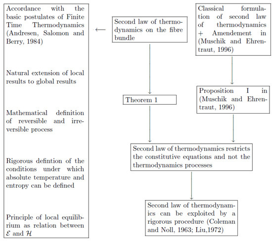  Figure 1. A schematized explanation of the analysis of the entropy principle developed in the present paper, and of its relation to the Muschik and Ehrentraut theory. An Amendment to second law of thermodynamics has been proposed by Muschik and Ehrentraut in 1996 [13]; rigorous procedures for the exploitation of the entropy principle have been formulated by Coleman and Noll in 1963 [1], and by Liu in 1972 [12]; the general tenets of Finite Time Thermodynamics have been summarized by Andresen, Salomon and Berry in 1984 [17].

In reference [21], the results in [13] were extended in order to encompass non-regular processes. Such an investigation deserves consideration, since thermodynamic processes involving discontinuous solutions are frequent in physics. In future research studies, we will aim to reanalyze the results in [21], within the mathematical framework presented here.

References

- Coleman, B.D.; Noll, W. The thermodynamics of elastic materials with heat conduction and viscosity. Arch. Ration. Mech. Anal. 1963, 13, 167–178. [Google Scholar] [CrossRef]
- Truesdell, C. Rational Thermodynamics, 2nd ed.; Springer: New York, NY, USA, 1984. [Google Scholar]
- Grad, H. On the kinetic theory of rarefied gases. Commun. Pure Appl. Math. 1949, 2, 331–407. [Google Scholar] [CrossRef]
- Jou, D.; Casas-Vázquez, J.; Lebon, G. Extended Irreversible Thermodynamics, 4th ed.; Springer: Berlin, Germany, 2010. [Google Scholar]
- Müller, I.; Ruggeri, T. Rational Extended Thermodynamics, 2nd ed.; Springer: New York, NY, USA, 1998. [Google Scholar]
- Sellitto, A.; Cimmelli, V.A.; Jou, D. Mesoscopic Theories of Heat Transport in Nanosystems; Springer: Berlin, Germany, 2016. [Google Scholar]
- Szucs, M.; Kovacs, R.; Simic, S. Open Mathematical Aspects of Continuum Thermodynamics: Hyperbolicity, Boundaries and Nonlinearities. Symmetry 2020, 12, 1469. [Google Scholar] [CrossRef]
- Smith, G.F. On isotropic functions of symmetric tensors, skew-symmetric tensors and vectors. Int. J. Eng. Sci. 1971, 9, 899–916. [Google Scholar] [CrossRef]
- Oliveri, F. Lie Symmetries of Differential Equations: Classical Results and Recent Contributions. Symmetry 2010, 2, 658–706. [Google Scholar] [CrossRef] [Green Version]
- Cimmelli, V.A.; Jou, D.; Ruggeri, T.; Ván, P. Entropy Principle and Recent Results in Non-Equilibrium Theories. Entropy 2014, 16, 1756–1807. [Google Scholar] [CrossRef] [Green Version]
- Triani, V.; Papenfuss, C.; Cimmelli, V.A.; Muschik, W. Exploitation of the Second Law: Coleman-Noll and Liu Procedure in Comparison. J. Non-Equilib. Thermodyn. 2008, 33, 47–60. [Google Scholar] [CrossRef] [Green Version]
- Liu, I.-S. Method of Lagrange multipliers for exploitation of the entropy principle. Arch. Ration. Mech. Anal. 1972, 46, 131–148. [Google Scholar] [CrossRef]
- Muschik, W.; Ehrentraut, H. An Amendment to the Second Law. J. Non-Equilib. Thermodyn. 1996, 21, 175–192. [Google Scholar] [CrossRef]
- Dolfin, M.; Francaviglia, M.; Rogolino, P. A Geometric Perspective on Irreversible Thermodynamics with Internal Variables. J. Non-Equilib. Thermodyn. 1998, 23, 250–263. [Google Scholar] [CrossRef]
- Dolfin, M.; Francaviglia, M.; Rogolino, P. A geometric model for the thermodynamics of simple materials. Period. Polytech. Mech. Eng. 1999, 43, 29–37. [Google Scholar]
- Andresen, B.; Berry, R.S.; Nitzan, A.; Salomon, P. Thermodynamics in finite time. I. The step-Carnot cicle. Phys. Rev. A 1977, 15, 2086–2093. [Google Scholar] [CrossRef]
- Andresen, B.; Salomon, P.; Berry, R.S. Thermodynamics in finite time. Phys. Today 1984, 37, 62–70. [Google Scholar] [CrossRef]
- Hoffmann, K.H. Recent Developments in Finite Time Thermodynamics. Tech. Mech. 2002, 22, 14–25. [Google Scholar]
- De Groot, S.R.; Mazur, P. Nonequilibrium Thermodynamics; North-Holland Publishing Company: Amsterdam, The Netherlands, 1962. [Google Scholar]
- Courant, R.; Hilbert, D. Methods of Mathematical Physics: Partial Differential Equations; John Wiley and Sons: New York, NY, USA, 1989; Volume II. [Google Scholar]
- Triani, V.; Cimmelli, V.A. Interpretation of Second Law of Thermodynamics in the presence of interfaces. Contin. Mech. Thermodyn. 2012, 24, 165–174. [Google Scholar] [CrossRef]
Publisher’s Note: MDPI stays neutral with regard to jurisdictional claims in published maps and institutional affiliations. |
© 2022 by the authors. Licensee MDPI, Basel, Switzerland. This article is an open access article distributed under the terms and conditions of the Creative Commons Attribution (CC BY) license (https://creativecommons.org/licenses/by/4.0/).