Skorokhod Reflection Problem for Delayed Brownian Motion with Applications to Fractional Queues

Abstract

Several queueing systems in heavy traffic regimes are shown to admit a diffusive approximation in terms of the Reflected Brownian Motion. The latter is defined by solving the Skorokhod reflection problem on the trajectories of a standard Brownian motion. In recent years, fractional queueing systems have been introduced to model a class of queueing systems with heavy-tailed interarrival and service times. In this paper, we consider a subdiffusive approximation for such processes in the heavy traffic regime. To do this, we introduce the Delayed Reflected Brownian Motion by either solving the Skorohod reflection problem on the trajectories of the delayed Brownian motion or by composing the Reflected Brownian Motion with an inverse stable subordinator. The heavy traffic limit is achieved via the continuous mapping theorem. As a further interesting consequence, we obtain a simulation algorithm for the Delayed Reflected Brownian Motion via a continuous-time random walk approximation.

1. Introduction

Queueing theory is a widely studied branch of mathematics, thanks to its numerous applications. Aside from the classical ones in telecommunications [1] and traffic engineering [2], one can cite the ones in computing [3] (with particular attention to scheduling) and economics (see, for instance, [4]), together with the fact that such a branch clearly shares different models with population dynamics (see also [5]). The simplest building block of such a theory is given by the $M/M/1$ queue, which is the prototype of a Markovian queueing model. While, on one hand, the study of this queueing model at its stationary phase can be achieved without too much effort (see, for instance, [6,7]), the determination of its distribution during the transient phase is a quite difficult task that requires much more attention (see, for instance, [8,9]).

The main feature of the $M/M/1$ queue is the Markov property, which, on one hand, gives a quite tractable model, while, on the other, it precludes any possibility of including memory effects. To overcome such a problem, one can extend the study to the class of semi-Markov processes, introduced by Lévy in [10]. A special class of semi-Markov processes can be obtained by means of a time change, i.e., the introduction of a non-Markov stochastic clock in the model. This is done, for instance, by composing a parent Markov process with the inverse of a subordinator. In the specific case of the $\alpha$-stable subordinator, one refers to such a new process as a fractional version of the parent one, due to the link between this time-change procedure and fractional calculus, as one can see from [11,12,13,14,15,16,17], to cite some of the several works on the topic. Together with a purely mathematical interest, let us stress that this procedure leads also to some interesting applications (see, for instance, [18] in economics, [19] in computing and [20] in computational neurosciences). In the context of queueing theory, this has been first done in [4], in the case of the $M/M/1$ queue, and then extended in [21,22] to the case of $M/M/1$ queues with catastrophes, [23] in the case of Erlang queues and [24] for the $M/M/\infty$ queues.

Another quite interesting feature of the classical $M/M/1$ queue is given by its link with the Brownian motion. It is well known that the behavior of the queue is widely influenced by the traffic intensity $\rho$. In particular, if $\rho <1$, the queue is ergodic (and thus admits a stationary state), while for $\rho \ge 1$, this is no longer true. In a certain sense, we can see the critical value $\rho =1$ as a bifurcation of the system (as seen as some sort of integral curve in the space of probability measures), in which it loses its globally asymptotically stable equilibrium point. Thus, a natural question one can ask concerns what happens, at a proper scaling, to the queueing model as $\rho$ is near 1. This is called the heavy traffic regime. In the case of the $M/M/1$ queue, it is well known that, up to a proper scaling, the queue length process in the heavy traffic regime can be approximated by means of a Reflected Brownian Motion with negative drift (see [25]), i.e., a Brownian motion with negative drift whose velocity is symmetrically regulated as soon as it touches 0. More precisely, the Reflected Brownian Motion is the solution of the Skorokhod reflection problem on the trajectory of a drifted Brownian motion. This process is of independent importance, as it provides the stochastic representation of the solution of the heat equation with Neumann boundary condition (see [26]).

The time-change procedure described before has been also applied to the Brownian motion, obtaining the so-called Delayed Brownian Motion (see [27]). Despite the name, it is interesting to observe that such a process is not necessarily delayed: it is true that it exhibits some intervals of constancy; nevertheless, on short times, it can vary faster than the parent Brownian motion, as evidenced from its expected lifetime in fractal sets (see [28]). Once this procedure has been applied to the Brownian motion, one could ask what happens as we adopt a time-change also to the Reflected Brownian Motion.

In this paper, we introduce the Delayed Reflected Brownian Motion (DRBM) as the solution of the Skorokhod reflection problem for the trajectories of the Delayed Brownian Motion (DBM). In particular, we prove that the process obtained in this way coincides with the one achieved by time-changing the Reflected Brownian Motion via an inverse stable subordinator. As a consequence, we can obtain some alternative representations of the process as a direct counterpart of the ones in the classical case. Among them, it is interesting to cite that we are able to exhibit a representation analogous to the one of [29] in terms of time-changed stochastic differential equations (introduced in [30]). We then use such a process to characterize the heavy traffic regime of a fractional $M/M/1$ queue. The results that we obtain have a twofold interest. One one hand, we achieve a subdiffusive approximation of the fractional $M/M/1$ queue in the heavy traffic regime, which is a quite powerful tool to study the properties of such queueing models. On the other hand, if we take a look at the results from a different point of view, we have a continuous-time random walk approximation of the Delayed Reflected Brownian Motion. The latter can be used to provide simulation algorithms that do not require us to simulate the inverse subordinator or to provide some inverse Laplace transforms (both of them being expensive computational tasks in terms of errors and time). The motivation of the paper is indeed in this twofold result: we want to provide a new tool to study the properties of the fractional $M/M/1$ queue introduced in [4] in the heavy traffic regime, while, at the same time, exploiting and better investigating the power of the discrete event simulation algorithm (see [31]) via continuous-time random walk approximations of a subdiffusive process.

The paper is organized as follows: in Section 2, we introduce the Skorokhod’s reflection problem and the Reflected Brownian Motion, while in Section 3, we investigate the Delayed Reflected Brownian Motion, with particular attention to the scaling properties of the two processes. The heavy traffic approximation for both the classical and the fractional $M/M/1$ queues is discussed in Section 4, together with some scaling properties of the classical $M/M/1$ queueing system. In this section, we also refine (and, in a certain sense, complete) the analysis of the queueing model introduced in [4], by proving the respective independence of the interarrival and the service times (recall that they are not mutually independent) and providing their distributions (with a different strategy with respect to [21] that does not require any further conditioning). Finally, in Section 5, we exhibit the simulation algorithm for the fractional $M/M/1$ queue and how to use it to simulate a Delayed Reflected Brownian motion, together with some heuristic considerations on stopping criteria.

2. The Reflected Brownian Motion

2.1. Skorokhod’s Reflection Problem

Let us denote by $C\left({\mathbb{R}}_0^{+}\right)$ (where ${\mathbb{R}}_0^{+}:=[0,+\infty )$) the space of continuous functions $f:{\mathbb{R}}_0^{+}\to \mathbb{R}$. In the following, we also need the space of cádlág functions $D\left({\mathbb{R}}_0^{+}\right)$, i.e., the space of functions $f:{\mathbb{R}}_0^{+}\to \mathbb{R}$ that are right-continuous and such that the left limits exist finite. Let us denote, for simplicity, $D_0\left({\mathbb{R}}_0^{+}\right):=\{y\in D\left({\mathbb{R}}_0^{+}\right):y\left(0\right)\ge 0\}$ and $C_0\left({\mathbb{R}}_0^{+}\right):=\{y\in C\left({\mathbb{R}}_0^{+}\right):y\left(0\right)\ge 0\}$, which are convex cones. Let us also recall that any monotone function $a:{\mathbb{R}}_0^{+}\to \mathbb{R}$ is locally of bounded variation and thus admits a distributional derivative ${\phantom{(}\mathrm{d}}^{}a$ that is a Radon measure (see [32]).

Definition 1.

Let $y\in D_0\left({\mathbb{R}}_0^{+}\right)$. We say that a pair $(z,a)\in D\left({\mathbb{R}}_0^{+}\right)\times D\left({\mathbb{R}}_0^{+}\right)$ is a solution of the one-dimensional Skorokhod reflection problem if

(i)

$z=y+a$;

(ii)

$z\left(t\right)\ge 0$ for any $t\ge 0$;

(iii)

a is nondecreasing, $a\left(0\right)=0$ and ${\phantom{(}\mathrm{d}}^{}a$ is supported on $\{s\in {\mathbb{R}}_0^{+}:z\left(s\right)=0\}$

Practically, we are asking if it is possible to construct a path z starting from y by adding a term a in such a way that whenever y touches 0, it is instantaneously symmetrically reflected (by using the function a), so that the resulting path z is conditioned to remain non-negative. For these reasons, the function a is called the regulator, while z is called the regulated path. Let us emphasize that the problem can be extended to the n-dimensional setting for any $n\in \mathbb{N}$—for instance, asking that the regulated path is conditioned to remain in a certain orthant (so that the path is symmetrically reflected as soon as it touches a coordinate hyperplane) or a polyedral region; see [33]. Let us recall that the one-dimensional Skorokhod problem admits a unique solution.

Theorem 1.

Let $y\in D_0\left({\mathbb{R}}_0^{+}\right)$. Then, there exists a unique solution $(z,a)\in D\left({\mathbb{R}}_0^{+}\right)\times D\left({\mathbb{R}}_0^{+}\right)$ of the one-dimensional Skorokhod reflection problem (given in Definition 1). In particular,

$$a\left(t\right)=\underset{s\le t}{sup}{y}^{-}\left(s\right)$$

where $y^{-}\left(t\right)=max\{-y\left(t\right),0\}$. Moreover, if $y\in C_0\left({\mathbb{R}}_0^{+}\right)$, then $(z,a)\in C\left({\mathbb{R}}_0^{+}\right)\times C\left({\mathbb{R}}_0^{+}\right)$.

With the previous theorem in mind, one can define the reflection map as $\mathrm{\Psi }:D_0\left({\mathbb{R}}_0^{+}\right)\to D\left({\mathbb{R}}_0^{+}\right)$ such that, for any $y\in D_0\left({\mathbb{R}}_0^{+}\right)$, $\mathrm{\Psi }\left(y\right)=z$, where $(z,a)$ is the unique solution of the Skorokhod problem. We also have that $\mathrm{\Psi }:C_0\left({\mathbb{R}}_0^{+}\right)\to C\left({\mathbb{R}}_0^{+}\right)$ is well defined.

Concerning the continuity of the reflection map on $D_0\left({\mathbb{R}}_0^{+}\right)$, we first have to consider some topology on it (see [25] (Chapter 3)).

Definition 2.

Let us consider the space $D\left(\right[0,T\left]\right)$ of the cádlág functions $f:[0,T]\to \mathbb{R}$. We denote by U the uniform topology, induced on $D\left(\right[0,T\left]\right)$ by the metric

$$d_U(x_1,x_2)=\underset{t\in [0,T]}{sup}|x_1\left(t\right)-x_2\left(t\right)|,x_1,x_2\in D\left([0,T]\right).$$

Let us denote by ι the identity map on $[0,T]$, i.e., $\iota \left(t\right)=t$ for any $t\in [0,T]$. Moreover, let

$$\mathrm{\Lambda }\left(\right[0,T\left]\right)=\{\lambda :[0,T]\to [0,T]:\lambda is strictly incrasing and \lambda (0)=0,\lambda (T)=T\}.$$

We denote by $J_1$ the topology on $D\left(\right[0,T\left]\right)$ defined by the metric

$$d_{J_1}(x_1,x_2)=\underset{\lambda \in \mathrm{\Lambda }\left(\right[0,T\left]\right)}{inf}max\{d_U(x_1\circ \lambda ,x_2),d_U(\lambda ,\iota )\},x_1,x_2\in D\left([0,T]\right),$$

where $\circ :D\left(\right[0,T\left]\right)\times D\left(\right[0,T\left]\right)\to D\left(\right[0,T\left]\right)$ is the composition map, i.e.,

$$(x_1\circ x_2)\left(t\right):=\circ (x_1,x_2)\left(t\right)=x_1\left(x_2\left(t\right)\right),t\in [0,T],x_1,x_2\in D\left([0,T]\right).$$

We denote by $x_n\stackrel{U}{\to }x$ and $x_n\stackrel{J_1}{\to }x$ the convergence in $D\left(\right[0,T\left]\right)$, respectively, in U and $J_1$. It is clear that if $x_n\stackrel{U}{\to }x$, then $x_n\stackrel{J_1}{\to }x$. We say that $x_n\stackrel{J_1}{\to }x$ in $D\left({\mathbb{R}}_0^{+}\right)$ if $x_n\stackrel{J_1}{\to }x$ in $D\left([0,T_k]\right)$ for a sequence ${\left\{T_k\right\}}_{k\ge 0}$ of continuity points of x such that $T_k\to +\infty$. This topology is metrizable and we still denote the metric as $d_{J_1}$.

In general, if we have a sequence of $D\left({\mathbb{R}}_0^{+}\right)$-valued random variables, we denote $X_n\Rightarrow X$ whenever $X_n$ converges in distribution to a $D\left({\mathbb{R}}_0^{+}\right)$-valued random variable X with respect to the $J_1$ topology.

Now, we can describe the continuity properties of the reflection map (see [25] (Lemma $\mathrm{13.5.1}$ and Theorem $\mathrm{13.5.1}$) for the compact domain case and extend it with [25] (Theorem $\mathrm{12.9.4}$) to the non-compact domain case).

Theorem 2.

The map $\mathrm{\Psi }:D_0\left([0,T]\right)\to D\left([0,T]\right)$ is Lipschitz-continuous in both U and $J_1$ topology with Lipschitz constant 2, i.e.,

$$d_U(\mathrm{\Psi }\left(x_1\right),\mathrm{\Psi }\left(x_2\right))\le 2d_U(x_1,x_2)$$

and

$$d_{J_1}(\mathrm{\Psi }\left(x_1\right),\mathrm{\Psi }\left(x_2\right))\le 2d_{J_1}(x_1,x_2).$$

(1)

Moreover, $\mathrm{\Psi }:D_0\left([0,+\infty )\right)\to D\left([0,+\infty )\right)$ is Lipschitz-continuous in the $J_1$ topology with Lipschitz constant 2, i.e., Equation (1) still holds in this case.

Let us also denote

$$\tilde{\mathrm{\Lambda }}=\{\lambda :{\mathbb{R}}_0^{+}\to {\mathbb{R}}_0^{+}:\lambda \mathrm{is} \mathrm{continuous}, \mathrm{nondecreasing} \mathrm{and} \lambda \left(0\right)=0\}$$

and observe the following elementary properties of the reflection map (which are particular cases of [25] (Lemma 13.5.2)).

Lemma 1.

The following properties are true:

(i)

For any $x\in D_0\left({\mathbb{R}}_0^{+}\right)$ and $b>0$, it holds that

$$\mathrm{\Psi }\left(bx\right)=b\mathrm{\Psi }\left(x\right);$$

(ii)

For any $x\in D_0\left({\mathbb{R}}_0^{+}\right)$ and $\lambda \in \tilde{\mathrm{\Lambda }}$, it holds that

$$\mathrm{\Psi }(x\circ \lambda )=\mathrm{\Psi }\left(x\right)\circ \lambda .$$

Proof. 

Let us first observe that, clearly, ${\left(bx\right)}^{-}=b{x}^{-}$. Then it holds, for any $t\ge 0$, by Theorem 1, that

$$\mathrm{\Psi }\left(bx\right)\left(t\right)=bx\left(t\right)+\underset{s\le t}{sup}{\left(bx\right)}^{-}\left(s\right)=b(x\left(t\right)+\underset{s\le t}{sup}{x}^{-}\left(s\right))=b\mathrm{\Psi }\left(x\right)\left(t\right),$$

proving property (i).

Concerning property (ii), let us observe that ${(x\circ \lambda )}^{-}=x^{-}\circ \lambda$. Define the running supremum $a\left(x\right)\left(t\right)={sup}_{s\le t}x\left(s\right)$ for any $t\ge 0$. Then, $a\left(x^{-}\right)\in D\left({\mathbb{R}}_0^{+}\right)$ by Theorem 1. Moreover, we have $a\left(x^{-}\right)\circ \lambda =a(x^{-}\circ \lambda )$. Indeed, let us define the set $\mathcal{F}$ of maps $f:{\mathbb{R}}_0^{+}\to 2^{\mathbb{R}}$ and the range map $\mathcal{R}:D\left({\mathbb{R}}_0^{+}\right)\to \mathcal{F}$ as $\mathcal{R}\left(z\right)\left(t\right)=\{y\in \mathbb{R}:\exists s\le t:z(s)=y\}$ for any $t\ge 0$ and any $z\in D\left({\mathbb{R}}_0^{+}\right)$. Then, $\lambda$ being increasing and continuous, we have

$$\begin{array}{cc}\hfill \mathcal{R}(x^{-}\circ \lambda )\left(t\right)& =\{y\in \mathbb{R}:\exists s\le t:x^{-}\left(\lambda \left(s\right)\right)=y\}\hfill \\ \hfill & =\{y\in \mathbb{R}:\exists \lambda \left(s\right)\le \lambda \left(t\right):x^{-}\left(\lambda \left(s\right)\right)=y\}\hfill \\ \hfill & =\{y\in \mathbb{R}:\exists \tau \le \lambda \left(t\right):x^{-}\left(\tau \right)=y\}=\mathcal{R}\left(x^{-}\right)\left(\lambda \left(t\right)\right).\hfill \end{array}$$

Hence,

$$a(x^{-}\circ \lambda )\left(t\right)=sup\mathcal{R}(x^{-}\circ \lambda )\left(t\right)=sup\mathcal{R}\left(x^{-}\right)\left(\lambda \left(t\right)\right)=a\left(x^{-}\right)\left(\lambda \left(t\right)\right)$$

and finally

$$\begin{array}{cc}\hfill \mathrm{\Psi }(x\circ \lambda )\left(t\right)& =x\left(\lambda \left(t\right)\right)+a(x^{-}\circ \lambda )\left(t\right)\hfill \\ \hfill & =x\left(\lambda \left(t\right)\right)+a\left(x^{-}\right)\left(\lambda \left(t\right)\right)=\mathrm{\Psi }\left(x\right)\left(\lambda \left(t\right)\right).\hfill \end{array}$$

   □

2.2. The Reflected Brownian Motion

Let us fix a complete filtered probability space $(\mathrm{\Omega },\mathcal{F},{\left\{{\mathcal{F}}_t\right\}}_{t\ge 0},\mathbb{P})$, supporting all the following random variables and processes. Let $W=\left\{W\right(t),t\ge 0\}$ be a standard Brownian motion and $W^{\eta ,{\sigma }^2}=\{W^{\eta }\left(t\right),t\ge 0\}$ be the Brownian motion with drift $\eta \in \mathbb{R}$ and diffusion parameter ${\sigma }^2$ with $\sigma >0$ (we denote it as $W^{\eta ,{\sigma }^2}\sim \mathrm{BM}(\eta ,{\sigma }^2)$) defined as

$$W^{\eta ,{\sigma }^2}\left(t\right)=\sigma W\left(t\right)+\eta t,t\ge 0.$$

If $\sigma =1$, we denote $W^{\eta }\sim \mathrm{BM}\left(\eta \right)$, and if, additionally, $\eta =0$, we denote $W\sim \mathrm{BM}$. In any case, we set $\mathbb{P}(W^{\eta ,{\sigma }^2}\left(0\right)=0)=1$. It is well known that $\mathbb{P}(W^{\eta ,{\sigma }^2}\in C\left({\mathbb{R}}_0^{+}\right))=1$; thus, we can solve the Skorokhod problem on each sample path of $W^{\eta ,{\sigma }^2}$.

Definition 3.

The Reflected Brownian Motion (RBM) with drift η and diffusion parameter ${\sigma }^2$ is given by the process ${\tilde{W}}^{\eta ,{\sigma }^2}=\{{\tilde{W}}^{\eta ,{\sigma }^2}\left(t\right),t\ge 0\}$ defined as

$${\tilde{W}}^{\eta ,{\sigma }^2}=\mathrm{\Psi }\left(W^{\eta ,{\sigma }^2}\right),$$

and we denote ${\tilde{W}}^{\eta ,{\sigma }^2}\sim \mathrm{RBM}(\eta ,{\sigma }^2)$. If ${\sigma }^2=1$, we denote it by ${\tilde{W}}^{\eta }\sim \mathrm{RBM}\left(\eta \right)$. If additionally $\eta =0$, we denote it by $\tilde{W}\sim \mathrm{RBM}$.

It is clear, by definition, that an RBM is almost surely non-negative. This is achieved thanks to the regulator, which provides a symmetrization of the velocity with which the original BM tries to cross 0. This additive component symmetrizes perfectly such an effort, thus preventing the process from crossing the 0 threshold. However, in this case, the regulator is a singular function; thus, we cannot properly speak about velocity. The symmetrizing effect of the regulator is instead clearer in the processes that are linked to the queueing systems, as will be shown in Section 4. First, we want to prove a simple scaling property. To do this, let us denote ${\iota }_b\in \tilde{\mathrm{\Lambda }}$ as ${\iota }_b\left(t\right)=bt$. Obviously, ${\iota }_1\equiv \iota$. Extending the arguments in [25] (Theorem $\mathrm{5.7.9}$), we have the following result.

Proposition 1.

Let ${\tilde{W}}^{\eta ,{\sigma }^2}\sim \mathrm{RBM}(\eta ,{\sigma }^2)$. The following properties hold true.

(i)

For any $b,c>0$, it holds that

$$c{\tilde{W}}^{\eta ,{\sigma }^2}\circ {\iota }_b\sim \mathrm{RBM}(\eta bc,{\sigma }^2{c}^{2}b);$$

(ii)

If $\eta \ne 0$, it holds that

$${\tilde{W}}^{\eta ,{\sigma }^2}\stackrel{d}{=}\frac{{\sigma }^2}{\left|\eta \right|}{\tilde{W}}^{sign\left(\eta \right)}\circ {\iota }_{\frac{{\eta }^2}{{\sigma }^2}};$$

(iii)

If $\eta =0$, it holds that

$${\tilde{W}}^{0,{\sigma }^2}\stackrel{d}{=}\tilde{W}\circ {\iota }_{{\sigma }^2}$$

(iv)

If $\eta =0$, it holds that

$${\tilde{W}}^{0,{\sigma }^2}\stackrel{d}{=}\sigma \tilde{W}.$$

Proof. 

Let us first prove property (i). Consider $W^{\eta ,{\sigma }^2}\sim \mathrm{BM}(\eta ,{\sigma }^2)$ such that ${\tilde{W}}^{\eta ,{\sigma }^2}=\mathrm{\Psi }\left({\tilde{W}}^{\eta ,{\sigma }^2}\right)$. The self-similarity of the Brownian motion implies that

$$\begin{array}{c}\hfill c{W}^{\eta ,{\sigma }^2}\circ {\iota }_b=c\sigma W\circ {\iota }_b+{\iota }_{c\eta b}\stackrel{d}{=}c\sigma \sqrt{b}W+{\iota }_{c\eta b}=W^{\eta bc,{\sigma }^2{c}^{2}b}.\end{array}$$

Applying the reflection map on both sides, we conclude the proof by Lemma 1.

Property (ii) follows from property (i) applied on ${\tilde{W}}^{sign\left(\eta \right)}$ by choosing $b=\frac{{\eta }^2}{{\sigma }^2}$ and $c=\frac{{\sigma }^2}{\left|\eta \right|}$. Property (iii) follows from property (i) applied on $\tilde{W}$ by choosing $b={\sigma }^2$ and $c=1$. Finally, property (iv) follows from (i) applied on $\tilde{W}$ by choosing $b=1$ and $c=\sigma$.    □

From now on, we will focus on the case ${\sigma }^2=1$, as any other case can be deduced from this one. Let us stress that the one-dimensional distribution of ${\tilde{W}}^{\eta }$ is well known (see [25] (Theorem $\mathrm{5.7.7}$) or [34] (Section $3.6$)).

Theorem 3.

For ${\tilde{W}}^{\eta }\sim \mathrm{RBM}\left(\eta \right)$, $y\ge 0$ and $t>0$, it holds that

$$\mathbb{P}({\tilde{W}}^{\eta }\left(t\right)>y)=\mathrm{\Phi }\left(\frac{-y+\eta t}{\sqrt{t}}\right)+e^{2\eta y}\mathrm{\Phi }\left(\frac{-y-\eta t}{\sqrt{t}}\right),$$

where Φ is the cumulative distribution function (CDF) of a standard normal random variable, i.e.,

$$\mathrm{\Phi }\left(x\right)=\frac{1}{\sqrt{2\pi }}{\int }_{-\infty }^x{e}^{-\frac{y^2}{2}}dy,x\in \mathbb{R}.$$

Remark 1.

It is clear that $\mathbb{P}({\tilde{W}}^{\eta }\left(t\right)>y)=1$ for any $y<0$ by definition. Let us also observe that, if $\eta =0$, then the one-dimensional distribution of $\tilde{W}$ is a folded Gaussian distribution. This will be made clearer in the following subsection.

As a consequence of the previous theorem, we have the following corollary (see [35] (Corollary 1.1.1)).

Corollary 1.

For ${\tilde{W}}^{\eta }\sim \mathrm{RBM}\left(\eta \right)$ with $\eta <0$ and $t>0$, it holds that

$$\mathbb{E}\left[{\tilde{W}}^{\eta }\left(t\right)\right]=\frac{1}{2\left|\eta \right|}-\frac{({\eta }^{2}t+1)}{\left|\eta \right|}(1-\mathrm{\Phi }(\left|\eta \right|\sqrt{t}\left)\right)+\sqrt{t}\phi \left(\right|\eta |\sqrt{t}),$$

where φ is the probability density function (PDF) of a standard normal random variable, i.e.,

$$\phi \left(x\right)={\mathrm{\Phi }}^{\prime }\left(x\right)=\frac{1}{\sqrt{2\pi }}{e}^{-\frac{x^2}{2}},x\in \mathbb{R}.$$

2.3. Alternative Construction of the Reflected Brownian Motion

One can provide a different construction of the Reflected Brownian Motion by means of the absolute value of an Itô process. To do this, let us observe, as done in [36], that, whenever $y\left(0\right)=0$, it holds that

$$\mathrm{\Psi }\left(y\right)\left(t\right)=\underset{s\le t}{sup}(y\left(t\right)-y\left(s\right)).$$

Using this characterization, together with the fact that $W^{\eta }\left(0\right)=0$, we have

$${\tilde{W}}^{\eta }\left(t\right)=\underset{s\le t}{sup}(\eta t+W\left(t\right)-\eta s-W\left(s\right))=\underset{s\le t}{sup}(-\eta (s-t)-(W\left(s\right)-W\left(t\right))).$$

It is clear that $\widehat{W}=-W$ is still a Brownian motion and we can write

$${\tilde{W}}^{\eta }\left(t\right)=\underset{s\le t}{sup}(-\eta (s-t)+(\widehat{W}\left(s\right)-\widehat{W}\left(t\right)))={\widehat{M}}^{-\eta }\left(t\right)-{\widehat{W}}^{-\eta }\left(t\right),$$

where ${\widehat{W}}^{-\eta }\sim \mathrm{BM}(-\eta )$ and ${\widehat{M}}^{-\eta }\left(t\right)={max}_{s\le t}{\widehat{W}}^{-\eta }\left(s\right)$ is the running maximum of ${\widehat{W}}^{-\eta }$. Combining the previous argument with [29] (Theorem 1), we get the following result.

Theorem 4.

For ${\tilde{W}}^{\eta }\sim \mathrm{RBM}\left(\eta \right)$, the following properties are true.

(i)

There exists a process $W^{-\eta }\sim \mathrm{BM}(-\eta )$ such that, denoting by $M^{-\eta }\left(t\right)={sup}_{s\le t}{W}^{-\eta }\left(s\right)$, it holds that

$${\tilde{W}}^{\eta }=M^{-\eta }-W^{-\eta }.$$

(ii)

Let $W\sim \mathrm{BM}$ and consider $X^{\eta }$ the unique strong solution of the stochastic differential equation

$$d{X}^{\eta }\left(t\right)=\eta sign\left(X^{\eta }\left(t\right)\right)dt+dW\left(t\right),X^{\eta }\left(0\right)=0.$$

(2)

Then, it holds that

$${\tilde{W}}^{\eta }\stackrel{d}{=}\left|X^{\eta }\right|.$$

Remark 2.

• In the case $\eta =0$, the previous theorem tells that $\tilde{W}\stackrel{d}{=}\left|W\right|$, i.e., it is a folded Gaussian process, as observed in the previous subsection.
• The equality in law $M^0-W\stackrel{d}{=}\left|W\right|$ has been proven by Lévy prior to [29]; see [37] (Chapter VI, Theorem $2.3$).

The previous characterization of the RBM can be fruitfully used for stochastic simulation. Indeed, Equation (2) can be discretized by means of the Euler scheme (see [38]), which is weakly convergent of order 1. On the other hand, one could also simulate ${\tilde{W}}^{\eta }$ by means of the reflection map. However, such an algorithm is weakly convergent of order $1/2$. In any case, one can provide not only algorithms with improved weak convergence order, but also exact simulation algorithms for ${\tilde{W}}^{\eta }\left(t\right)$ at some grid points $t\ge 0$ (see [39]). Other approaches to generate the sample paths of the RBM are based on the Gauss–Markov nature of the Drifted Brownian Motion (see [40,41]). There is also another approximate simulation method that makes use of a continuous-time random walk (CTRW) approximation. The latter is made clearer in Section 5.

3. The Reflected Brownian Motion Delayed by the Inverse Stable Subordinator

3.1. Inverse Stable Subordinators and Semi-Markov Processes

Let us first introduce the inverse stable subordinator. To do this, we recall the following definitions (we refer to [42,43,44]).

Definition 4.

For any $\alpha \in (0,1)$, a standard α-stable subordinator ${\sigma }_{\alpha }=\{{\sigma }_{\alpha }\left(t\right),t\ge 0\}$ is an increasing Lévy process with ${\sigma }_{\alpha }\left(0\right)=0$ almost surely (a.s.) and such that

$$\mathbb{E}\left[e^{-\lambda {\sigma }_{\alpha }\left(t\right)}\right]=e^{t{\lambda }^{\alpha }},t\ge 0,\lambda \ge 0.$$

(3)

We call the inverse α-stable subordinator the process $L_{\alpha }=\{L_{\alpha }\left(t\right),t\ge 0\}$ defined as

$$L_{\alpha }\left(t\right)=inf\{y\ge 0:{\sigma }_{\alpha }\left(y\right)>t\},t\ge 0.$$

We denote by $\mathcal{L}$ the Laplace transform operator, i.e., for a function $f\in L_{\mathrm{loc}}^1\left({\mathbb{R}}_0^{+}\right)$,

$$\mathcal{L}\left[f\right]\left(\lambda \right)={\int }_0^{+\infty }{e}^{-\lambda t}f\left(t\right)dt,$$

and

$$\mathrm{abs}\left(f\right)=inf\{\lambda \in \mathbb{R}:\mathcal{L}[f\left]\right(\lambda \left) \mathrm{is} \mathrm{well}\text{-}\mathrm{defined} \mathrm{and} \mathrm{finite}\right\},$$

the abscissa of convergence of f. It is well known that $\mathcal{L}\left[f\right]\left(\lambda \right)$ is well defined for any $\lambda >\mathrm{abs}\left(f\right)$ (see [45] (Proposition $\mathrm{1.4.1}$)).

In the following proposition, we recall some of the main properties of the stable subordinator and its inverse (see [44]).

Proposition 2.

Let $\alpha \in (0,1)$ and ${\sigma }_{\alpha }$ an α-stable subordinator with inverse $L_{\alpha }$. Then,

(i)

${\sigma }_{\alpha }$ is a strictly increasing process with a.s. pure jump sample paths;

(ii)

$L_{\alpha }$ is an increasing process with a.s. continuous sample paths;

(iii)

For any fixed $t>0$, ${\sigma }_{\alpha }\left(t\right)$ is an absolutely continuous random variable with PDF $g_{\alpha }(s;t)$ satisfying

$$g_{\alpha }(s;t)=t^{-\frac{1}{\alpha }}{g}_{\alpha }\left(s{t}^{-\frac{1}{\alpha }}\right),s>0,$$

where $g_{\alpha }(·):=g_{\alpha }(·;1)$. This means that ${\sigma }_{\alpha }\left(t\right)\stackrel{d}{=}{t}^{\frac{1}{\alpha }}{\sigma }_{\alpha }\left(1\right)$;

(iv)

For any fixed $t>0$, $L_{\alpha }\left(t\right)$ is an absolutely continuous random variable with PDF $f_{\alpha }(s;t)$ satisfying

$$f_{\alpha }(s;t)=\frac{t}{\alpha }{s}^{-1-\frac{1}{\alpha }}{g}_{\alpha }\left(t{s}^{-\frac{1}{\alpha }}\right),s>0;$$

(v)

For any fixed $s>0$, it holds that $\mathrm{abs}\left(f_{\alpha }(s;·)\right)=0$ and

$$\mathcal{L}\left[f_{\alpha }(s,·)\right]\left(\lambda \right)={\lambda }^{\alpha -1}{e}^{-s{\lambda }^{\alpha }},\lambda >0.$$

Remark 3.

Remark that, while ${\sigma }_{\alpha }$ is a Lévy process and then a strong Markov process, $L_{\alpha }$ is not even a Markov process.

As it is clear from the previous proposition, explicit formulae for the one-variable function $g_{\alpha }$ lead to analogous ones for the density of the stable subordinator and its inverse. However, such explicit formulae are not so easy to handle. First of all, there are several integral representations of $g_{\alpha }$ (see [46] and references therein). Among them, let us recall the so-called Mikusinski representation:

$$g_{\alpha }\left(s\right)=\frac{1}{\pi }\frac{\alpha }{1-\alpha }\frac{1}{s}{\int }_0^{\pi }{s}^{-\frac{\alpha }{1-\alpha }}{\left(\frac{sin\left(\alpha \tau \right)}{sin\left(\tau \right)}\right)}^{\frac{\alpha }{1-\alpha }}\frac{sin\left(\right(1-\alpha \left)\tau \right)}{sin\left(\tau \right)}{e}^{s^{-\frac{\alpha }{1-\alpha }}{\left(\frac{sin\left(\alpha \tau \right)}{sin\left(\tau \right)}\right)}^{\frac{\alpha }{1-\alpha }}\frac{sin\left(\right(1-\alpha \left)\tau \right)}{sin\left(\tau \right)}}d\tau .$$

This representation is shown to be quite useful both to determine asymptotic properties of $g_{\alpha }$ and to evaluate it numerically (see [47]). The function $g_{\alpha }$ can be also expressed in several ways as a function series (see [48]). Let us refer, among them, to the following formula:

$$g_{\alpha }\left(s\right)=\frac{1}{\pi }\sum _{j=1}^{\infty }\frac{{(-1)}^{j+1}}{j!s^{1+\alpha j}}\mathsf{\Gamma }(1+\alpha j)sin\left(\pi \alpha j\right).$$

The latter leads to a quite interesting representation of $f_{\alpha }(s;t)$, which can be also used to prove some regularity results (as, for instance, done in [49]). Further discussion on the various representations of $g_{\alpha }$ and $f_{\alpha }$ is given, for instance, in the Appendix of [50].

In the following, we want to apply a time-change procedure on $\tilde{W}$ by using as a stochastic clock the process $L_{\alpha }$. Thus, it could be useful to recall the notion of the semi-Markov process, as introduced in [10].

Definition 5.

A real valued cádlág process $X=\left\{X\right(t),t\ge 0\}$ is semi-Markov if, denoting by $\gamma =\left\{\gamma \right(t),t\ge 0\}$ its age process, i.e., $\gamma \left(t\right)=sup\{{\epsilon }_0>0:\forall \epsilon \in (0,{\epsilon }_0),X(t-\epsilon )=X\left(t\right)\}$, for any $0\le s<t$ and any $A\in \mathcal{B}\left(\mathbb{R}\right)$, where $\mathcal{B}\left(\mathbb{R}\right)$ is the Borel σ-algebra of $\mathbb{R}$, it holds that

$$\mathbb{P}(X\left(t\right)\in A|{\mathcal{F}}_s)=\mathbb{P}(X\left(t\right)\in A|X\left(s\right),\gamma \left(s\right)).$$

In particular, if we consider a strong Markov process $X=\left\{X\right(t),t\ge 0\}$ and an independent inverse $\alpha$-stable subordinator $L_{\alpha }$, we can define the time-changed process $X_{\alpha }=X\circ L_{\alpha }$. In [51], it is shown that, if we define the process $V:=\left\{V\right(t),t\ge 0\}$ as $V\left(t\right)=t-{\sigma }_{\alpha }(L_{\alpha }\left(t\right)-)$ for any $t\ge 0$, the couple $(X_{\alpha },V)$ is a strong Markov process. This implies (actually, it is equivalent) that $X_{\alpha }$ is a semi-Markov process. The semi-Markov property of $X_{\alpha }$, in particular, follows from the fact that $(X,{\sigma }_{\alpha })$ is a Markov additive process in the sense of [52] (see [51] for details). Finally, let us recall that such a semi-Markov property actually tells us that the process $X_{\alpha }$ satisfies a (strong) regenerative property (in the sense of [53]) with the regenerative set given by

$$\mathcal{M}:=\{s\ge 0:\exists t\ge 0,{\sigma }_{\alpha }\left(t\right)=s\},$$

i.e., the process $X_{\alpha }$ satisfies the strong Markov property on any random time $\mathcal{T}$ such that $\mathcal{T}\left(\omega \right)\in \mathcal{M}\left(\omega \right)$ for almost any $\omega \in \mathrm{\Omega }$. Actually, a regenerative property is common for any semi-Markov process and could be informally stated as follows: a semi-Markov process exhibits the strong Markov property at each time in which it changes its state.

3.2. The Reflected Brownian Motion Delayed by the Inverse Stable Subordinator

We are now ready to introduce the Delayed Reflected Brownian Motion.

Definition 6.

Let ${\tilde{W}}^{\eta ,{\sigma }^2}\sim \mathrm{RBM}(\eta ,{\sigma }^2)$, $\alpha \in (0,1)$ and $L_{\alpha }$ be an inverse stable subordinator independent of ${\tilde{W}}^{\eta ,{\sigma }^2}$. We define the Reflected Brownian Motion delayed by an inverse α-stable subordinator (DRBM) as the process ${\tilde{W}}_{\alpha }^{\eta ,{\sigma }^2}={\tilde{W}}^{\eta ,{\sigma }^2}\circ L_{\alpha }$, we denote it as ${\tilde{W}}_{\alpha }^{\eta ,{\sigma }^2}\sim \mathrm{DRBM}(\eta ,{\sigma }^2;\alpha )$ and we call ${\tilde{W}}^{\eta ,{\sigma }^2}$ its parent process. As before, if $\sigma =1$, we denote it as ${\tilde{W}}_{\alpha }^{\eta }\sim \mathrm{DRBM}(\eta ;\alpha )$, and if furthermore $\eta =0$, we denote it as ${\tilde{W}}_{\alpha }\sim \mathrm{DRBM}\left(\alpha \right)$.

First of all, let us stress that the arguments in the previous subsection tell us that ${\tilde{W}}_{\alpha }^{\eta ,{\sigma }^2}$ is semi-Markov. Together with ${\tilde{W}}_{\alpha }^{\eta ,{\sigma }^2}$, we can define the Delayed Brownian Motion $W_{\alpha }^{\eta ,{\sigma }^2}:=W^{\eta ,{\sigma }^2}\circ L_{\alpha }$, where $W^{\eta ,{\sigma }^2}\sim \mathrm{BM}(\eta ,{\sigma }^2)$ and $L_{\alpha }$ is an inverse $\alpha$-stable subordinator independent of it (see, for instance, [27]). We denote this as $W_{\alpha }^{\eta ,{\sigma }^2}\sim \mathrm{DBM}(\eta ,{\sigma }^2;\alpha )$ and we call $W^{\eta ,{\sigma }^2}$ its parent process.

Another natural definition for the DRBM could be obtained by simply considering $\mathrm{\Psi }\left(W_{\alpha }^{\eta ,{\sigma }^2}\right)$. In the following proposition, we observe that such a definition is equivalent to the one we have given.

Proposition 3.

Let $W_{\alpha }^{\eta ,{\sigma }^2}\sim \mathrm{DBM}(\eta ,{\sigma }^2;\alpha )$ with parent process $W^{\eta ,{\sigma }^2}$. Let ${\tilde{W}}^{\eta ,{\sigma }^2}=\mathrm{\Psi }\left(W^{\eta ,{\sigma }^2}\right)$ and ${\tilde{W}}_{\alpha }^{\eta ,{\sigma }^2}\sim \mathrm{DRBM}(\eta ,{\sigma }^2;\alpha )$ with parent process ${\tilde{W}}^{\eta ,{\sigma }^2}$. Then, ${\tilde{W}}_{\alpha }^{\eta ,{\sigma }^2}=\mathrm{\Psi }\left(W_{\alpha }^{\eta ,{\sigma }^2}\right)$ almost surely.

Proof. 

This proposition easily follows from property (ii) of Lemma 1 after observing that $\mathbb{P}(L_{\alpha }\in \tilde{\mathrm{\Lambda }})=1$.    □

Remark 4.

The couple $({\tilde{W}}_{\alpha }^{\eta ,{\sigma }^2},a\left({\left(W_{\alpha }^{\eta ,{\sigma }^2}\right)}^{-}\right))$ is the unique solution of the Skorokhod problem in Definition 1 for the sample paths of $W_{\alpha }^{\eta ,{\sigma }^2}$.

We can also deduce a scaling property for the DRBM in the spirit of Proposition 1.

Proposition 4.

Let ${\tilde{W}}_{\alpha }^{\eta ,{\sigma }^2}\sim \mathrm{DRBM}(\eta ,\sigma ;\alpha )$. The following properties hold true.

(i)

For any $c>0$, it holds that

$$c{\tilde{W}}_{\alpha }^{\eta ,{\sigma }^2}\sim \mathrm{DRBM}(\eta c,{\sigma }^2{c}^2;\alpha );$$

(ii)

It holds that

$${\tilde{W}}_{\alpha }^{\eta ,{\sigma }^2}\stackrel{d}{=}\sigma {\tilde{W}}_{\alpha }^{\eta /\sigma }.$$

Proof. 

Let us first show property (i). Let ${\tilde{W}}^{\eta ,{\sigma }^2}\sim \mathrm{RBM}(\eta ,{\sigma }^2)$ be the parent process of ${\tilde{W}}_{\alpha }^{\eta ,{\sigma }^2}$, and $L_{\alpha }$ be the involved inverse $\alpha$-stable subordinator. By Proposition 1 with $b=1$, we get $c{\tilde{W}}^{\eta ,{\sigma }^2}\sim \mathrm{RBM}\left(\eta c,{\sigma }^2{c}^2\right)$. By the Skorokhod representation theorem (see, for instance, [54]), we can suppose, without loss of generality, that there exists a process ${\tilde{W}}^{\eta c,{\sigma }^2{c}^2}\sim \mathrm{RBM}\left(\eta c,{\sigma }^2{c}^2\right)$ such that ${\tilde{W}}^{\eta c,{\sigma }^2{c}^2}=c{\tilde{W}}^{\eta ,{\sigma }^2}$ almost surely. This clearly implies that also ${\tilde{W}}^{\eta c,{\sigma }^2{c}^2}$ is independent of $L_{\alpha }$. Thus, composing both sides of the equality with $L_{\alpha }$, we conclude the proof of (i). Property (ii) follows from (i) applied to ${\tilde{W}}_{\alpha }^{\eta /\sigma }$ with $c=\sigma$.    □

Remark 5.

Thanks to the previous proposition, we can always reduce to the case ${\sigma }^2=1$. However, we cannot reduce to the case $\eta =\pm 1,0$. This is due to the fact that the composition operator is not symmetric and $L_{\alpha }\circ {\iota }_b\ne {\iota }_b\circ L_{\alpha }$ in general.

Thus, from now on, let us consider ${\sigma }^2=1$. Concerning the one-dimensional distribution, we get a subordination principle from a simple conditioning argument.

Proposition 5.

For ${\tilde{W}}_{\alpha }^{\eta }\sim \mathrm{DRBM}(\eta ,\alpha )$, $y\ge 0$ and $t>0$, it holds that

$$\mathbb{P}({\tilde{W}}_{\alpha }^{\eta }\left(t\right)>y|{\tilde{W}}_{\alpha }^{\eta }\left(0\right)=x)={\int }_0^{+\infty }\left(\mathrm{\Phi }\left(\frac{-y+\eta s}{\sqrt{s}}\right)+e^{2\eta y}\mathrm{\Phi }\left(\frac{-y-\eta s}{\sqrt{s}}\right)\right)f_{\alpha }(s;t)ds.$$

Proof. 

Let us rewrite $\mathbb{P}({\tilde{W}}_{\alpha }^{\eta }\left(t\right)>y|{\tilde{W}}_{\alpha }^{\eta }\left(0\right)=x)$ as a conditional expectation. Precisely, if we let ${\mathbf{1}}_A$ be the indicator function of the set $A\in \mathcal{B}\left(\mathbb{R}\right)$, that is to say,

$${\mathbf{1}}_A\left(x\right)=\left\{\begin{array}{cc}1\hfill & x\in A\hfill \\ 0\hfill & x\notin A,\hfill \end{array}\right.$$

it holds that

$$\begin{array}{cc}\hfill \mathbb{P}({\tilde{W}}_{\alpha }^{\eta }\left(t\right)>y)& =\mathbb{E}\left[{\mathbf{1}}_{(y,+\infty )}\left({\tilde{W}}_{\alpha }^{\eta }\left(t\right)\right)\right]=\mathbb{E}\left[{\mathbf{1}}_{(y,+\infty )}\left({\tilde{W}}^{\eta }\left(L_{\alpha }\left(t\right)\right)\right)\right],\hfill \end{array}$$

where ${\tilde{W}}^{\eta }$ is the parent process of ${\tilde{W}}_{\alpha }^{\eta }$ and $L_{\alpha }$ is independent of ${\tilde{W}}^{\eta }$. Using the tower property of conditional expectations, we achieve

$$\begin{array}{c}\hfill \mathbb{E}\left[{\mathbf{1}}_{(y,+\infty )}\left({\tilde{W}}^{\eta }\left(L_{\alpha }\left(t\right)\right)\right)\right]=\mathbb{E}\left[\mathbb{E}\left[{\mathbf{1}}_{(y,+\infty )}\left({\tilde{W}}^{\eta }\left(L_{\alpha }\left(t\right)\right)\right)\right|L_{\alpha }\left(t\right)]\right].\end{array}$$

We can set $\mathbb{E}\left[{\mathbf{1}}_{(y,+\infty )}\left({\tilde{W}}^{\eta }\left(L_{\alpha }\left(t\right)\right)\right)\right|L_{\alpha }\left(t\right)]=F\left(L_{\alpha }\left(t\right)\right)$ with   

$$\begin{array}{cc}\hfill F\left(s\right)& =\mathbb{E}\left[{\mathbf{1}}_{(y,+\infty )}\left({\tilde{W}}^{\eta }\left(L_{\alpha }\left(t\right)\right)\right)\right|L_{\alpha }\left(t\right)=s]\hfill \\ \hfill & =\mathbb{E}\left[{\mathbf{1}}_{(y,+\infty )}\left({\tilde{W}}^{\eta }\left(s\right)\right)\right]\hfill \\ \hfill & =\mathrm{\Phi }\left(\frac{-y+\eta s}{\sqrt{s}}\right)+e^{2\eta y}\mathrm{\Phi }\left(\frac{-y-\eta s}{\sqrt{s}}\right),\hfill \end{array}$$

where we also use the fact that $L_{\alpha }$ is independent of ${\tilde{W}}^{\eta }$ and Theorem 3. Finally, we have

$$\begin{array}{cc}\hfill \mathbb{E}\left[{\mathbf{1}}_{(y,+\infty )}\left({\tilde{W}}^{\eta }\left(L_{\alpha }\left(t\right)\right)\right)\right]& =\mathbb{E}\left[F\left(L_{\alpha }\left(t\right)\right)\right]\hfill \\ \hfill & ={\int }_0^{+\infty }F\left(s\right)f_{\alpha }(s;t)ds,\hfill \end{array}$$

concluding the proof.    □

With the same exact argument, we can prove the following statement.

Corollary 2.

For ${\tilde{W}}_{\alpha }^{\eta }\sim \mathrm{DRBM}\left(\eta \right)$ with $\eta <0$ and $t>0$, it holds that

$$\mathbb{E}\left[{\tilde{W}}_{\alpha }^{\eta }\left(t\right)\right]=\frac{1}{2\left|\eta \right|}-{\int }_0^{+\infty }\left(\frac{({\eta }^{2}s+1)}{\left|\eta \right|}(1-\mathrm{\Phi }(\left|\eta \right|\sqrt{s}\left)\right)+\sqrt{s}\phi \left(\right|\eta |\sqrt{s})\right)f_{\alpha }(s;t)ds.$$

As for the classical case, we could ask if there are some alternative representations of the DRBM in terms of the solution of some particular SDE. This is done by generalizing Theorem 4.

Theorem 5.

For ${\tilde{W}}_{\alpha }^{\eta }\sim \mathrm{DRBM}(\eta ;\alpha )$, the following properties are true.

(i)

There exists a process $W_{\alpha }^{-\eta }\sim \mathrm{DBM}(-\eta ;\alpha )$ such that, denoting by $M_{\alpha }^{-\eta }\left(t\right)={sup}_{s\le t}{W}_{\alpha }^{-\eta }\left(s\right)$ its running maximum, it holds that

$${\tilde{W}}_{\alpha }^{\eta }=M_{\alpha }^{-\eta }-W_{\alpha }^{-\eta }$$

almost surely.

(ii)

Let $W_{\alpha }\sim \mathrm{DBM}(\eta ;\alpha )$ and consider $X_{\alpha }^{\eta }$ the unique strong solution of the time-changed stochastic differential equation (in the sense of [30])

$$d{X}_{\alpha }^{\eta }\left(t\right)=\eta sign\left(X_{\alpha }^{\eta }\left(t\right)\right)d{L}_{\alpha }\left(t\right)+d{W}_{\alpha }\left(t\right),X_{\alpha }^{\eta }\left(0\right)=0.$$

(4)

Then, it holds that

$${\tilde{W}}_{\alpha }^{\eta }\stackrel{d}{=}\left|X_{\alpha }^{\eta }\right|.$$

Proof. 

Let us first prove property (i). Let ${\tilde{W}}^{\eta }$ be the parent process of ${\tilde{W}}_{\alpha }^{\eta }$. By item (i) of Theorem 4, we know that there exists $W^{-\eta }\sim \mathrm{BM}(-\eta )$ such that, setting $M^{-\eta }\left(t\right)={sup}_{s\le t}{W}^{-\eta }\left(s\right)$, it holds that

$${\tilde{W}}^{\eta }=M^{-\eta }-W^{-\eta }$$

(5)

Let $W_{\alpha }^{-\eta }\sim \mathrm{DBM}(-\eta ;\alpha )$ with parent process $W^{-\eta }$ and define $M_{\alpha }^{-\eta }$ as in the statement. Arguing as in Lemma 1, the fact that $\mathbb{P}(L_{\alpha }\in \tilde{\mathrm{\Lambda }})=1$ implies $M_{\alpha }^{-\eta }=M^{-\eta }\circ L_{\alpha }$ almost surely. Thus, applying the composition with $L_{\alpha }$ on both sides of equality (5), we conclude the proof of (i). To prove the second item, let us define $X^{\eta }$ as the unique strong solution of Equation (2), where W is the parent process of $W_{\alpha }$. Observe that, $L_{\alpha }$ being almost surely continuous, W is in synchronization with $L_{\alpha }$ (in the sense of [30] (p. 793)) and then we can use the duality theorem [30] (Theorem $4.2$) to state that $X_{\alpha }^{\eta }:=X^{\eta }\circ L_{\alpha }$ is the unique strong solution of

$$d{X}_{\alpha }^{\eta }\left(t\right)=\eta sign\left(X_{\alpha }^{\eta }(t-)\right)d{L}_{\alpha }\left(t\right)+d{W}_{\alpha }\left(t\right),X_{\alpha }^{\eta }\left(0\right)=0.$$

Continuity of $X_{\alpha }^{\eta }$ leads to Equation (4). Vice versa, if $X_{\alpha }^{\eta }$ is the unique strong solution of Equation (4), then the duality theorem tells us that $X^{\eta }$ is the unique strong solution of Equation (2). Thus, we observe that $X_{\alpha }^{\eta }$ is the unique strong solution of Equation (4) if and only if $X_{\alpha }^{\eta }=X^{\eta }\circ L_{\alpha }$, and the statement directly follows from item (ii) of Theorem 4.    □

One could try to use the previous characterization to provide an algorithm for the simulation of the DRBM. Such an approach requires, first of all, the simulation of a stable subordinator, which can be done by means of the Chambers–Mallow–Stuck algorithm [55], which is a generalization of the Box–Müller algorithm. As underlined in [43] (Section 5), one can simulate a time-changed process $X_{\alpha }=X\circ L_{\alpha }$ by setting a grid ${\left\{t_n\right\}}_{n\le N}$ (with $t_1<t_2<\cdots <t_N$), simulating ${\left\{{\sigma }_{\alpha }\left(t_n\right)\right\}}_{n\le N}$ and then the parent process X up to $t_N$. Finally, an approximate trajectory of the process $X_{\alpha }$ is obtained by a step plot between the nodes ${\left\{(X\left(t_n\right),{\sigma }_{\alpha }\left(t_n\right))\right\}}_{n\in N}$. Let us stress that such an algorithm can be generalized to any subordinator, but in this case, Laplace inversion could be required. Moreover, in the case of the DRBM, this involves the simulation of an RBM. We can bypass such a step by using a CTRW approximation of ${\tilde{W}}_{\alpha }^{\eta }$, at least for $\eta <0$. This follows from an analogous approach for the RBM, which will be discussed in the following sections.

4. Heavy Traffic Approximation of the Fractional $\mathit{M}/\mathit{M}/\mathbf{1}$ Queue

4.1. The Heavy Traffic Approximation of the Classical $M/M/1$ Queue

4.1.1. The Queueing Model

Let us first introduce the $M/M/1$ queueing model. Consider a system in which, at a certain average rate $\lambda$, a job (client) enters the system to be processed by a server, which takes a certain amount of time of mean $1/\mu$ to perform. If a job is currently being served and another job enters the system, it waits in line in a queue. Jobs that are waiting are then processed, as soon as the server is free, via a First In First Out (FIFO) policy. To model such a system, we assume in any case that the interarrival times (i.e., the time interval between the arrival of two jobs) are i.i.d. and so are the service times.

In this first case, i.e., the M/M/1 queueing system, we also suppose that:

• service times and interarrival times are independent of each other;
• the jobs enter the system following a Poisson arrival process;
• service times are exponentially distributed.

Thus, we consider two sequences $U={\left(U_k\right)}_{k\ge 1}$ and $V={\left(V_k\right)}_{k\ge 1}$ of i.i.d. exponential random variables of parameters, respectively, $\lambda >0$ and $\mu >0$ that are independent of each other, representing, respectively, the interarrival and the service times. We can define the sequence of the arrival times (i.e., the time instants in which the jobs enter the system) $S^U={\left(S_k^U\right)}_{k\ge 0}$ as

$$S_k^U=\sum _{j=1}^k{U}_j,$$

where we set $S_0^U=0$. Let $A=\left\{A\right(t),t\ge 0\}$ be the arrival counting process, i.e., $A\left(t\right)$ is the number of arrivals up to time t. It is defined as

$$A\left(t\right)=max\{k\ge 0:S_k^u\le t\}.$$

In the case of a M/M/1 system, as we supposed before, A is a Poisson process of parameter $\lambda$ and we denote it by $A\sim \mathrm{Pois}\left(\lambda \right)$. We can also define the sequence $S^V={\left(S_k^V\right)}_{k\ge 0}$, which is, for any $k\ge 0$, the total amount of time that is necessary to process the first k-th jobs, as 

$$S_k^V=\sum _{j=1}^k{V}_j,$$

where we set $S_0^V=0$, and the cumulative input process $C=\left\{C\right(t),t\ge 0\}$ as   

$$C\left(t\right)=\sum _{j=1}^{A\left(t\right)}{V}_j=S_{A\left(t\right)}^V,$$

i.e., the necessary service times to process all the tasks that entered the system up to time t. Let us stress that $S_k^V$ is not the time of completion of the k-th task, as there could have been some idle periods. By using the cumulative input process, we can introduce the net input process $X=\left\{X\right(t),t\ge 0\}$ as

$$X\left(t\right)=C\left(t\right)-t.$$

The net input process takes, in a certain sense, a balance between the total service time that is necessary to process all the tasks and the time that has passed since the system is initialized. By definition, X is a cádlág process that decreases with continuity while it increases only by jumping. Moreover, $X\left(0\right)=0$, and thus $X\in D_0\left({\mathbb{R}}_0^{+}\right)$ almost surely, and we can define the workload process $WL=\left\{WL\right(t),t\ge 0\}$ via the Skorokhod reflection map as $WL=\mathrm{\Psi }\left(X\right)$. One can visualize how $WL$ works: when it is positive, the process $WL$ decreases linearly with slope $-1$ until it reaches 0; once 0 has been reached, it remains constant (while the net input $X\left(t\right)$ could be still decreasing); each time X jumps, so does $WL$. Thus, it is clear that $WL$ is 0 during idle periods and it is positive while a job is being served. We can state that $WL$, in a certain sense, measures how much residual time is needed to process all the tasks. Here, the effect of the regulator is much clearer than in the RBM case. Indeed, the process $WL\left(t\right)$ tries to cross 0 with a fixed slope of $-1$. As soon as $WL\left(t\right)$ touches 0, the regulator symmetrizes such a slope, thus adding a linear term with slope 1 to the process. The sum of the symmetric effects of the proper velocity of $WL\left(t\right)$ (or, in other words, the effort that $X\left(t\right)$ puts into driving $WL\left(t\right)$ against 0) and the velocity of the regulator is the main motivation for which the process $WL\left(t\right)$ stabilizes on 0 until it increases jumping away. Such an example actually shows how the threshold 0 works as a mirror for the velocity of the process and how the regulator provides a symmetric additional term to such a velocity. Moreover, it is clear that, for any $t\ge 0$, it holds that $WL\left(t\right)\le C\left(t\right)$: they increase together with the same amount, but $WL$ decreases with continuity in the meantime. As C measures the total amount of necessary service time, up to time t, to process all the jobs, and $WL$, the remaining amount of time to process all the waiting jobs, up to time t, their difference represents the total amount of time, up to time t, in which the server was actually working. We call such a process the cumulative busy time process $B=\left\{B\right(t),t\ge 0\}$, where $B\left(t\right)=C\left(t\right)-WL\left(t\right)$. The cumulative busy time process is increasing and piecewise linear. It remains constant during idle periods; otherwise, it grows with slope 1. Thus, if we consider B as the clock of the process, we are only neglecting the idle periods. Thus, if we count service times only on this clock, we obtain the exact number of processed jobs. Hence, we consider a counting process $N=\left\{N\right(t),t\ge 0\}$ of the service times, i.e., 

$$N\left(t\right)=max\{k\ge 0:S_k^V\le t\},$$

and then we define the departure process $D=\left\{D\right(t),t\ge 0\}$ as $D\left(t\right)=N\left(B\right(t\left)\right)$. Finally, the balance between the number of arrivals and the number of departures, i.e., the number of jobs that are currently in the system, gives us the queue length process $Q=\left\{Q\right(t),t\ge 0\}$, i.e., $Q\left(t\right)=A\left(t\right)-D\left(t\right)$. Since we are mainly interested in the process Q, we resume the full construction with the notation $Q\sim \mathrm{M}/\mathrm{M}/1(\lambda ,\mu )$. In any case, we will adopt the full notation that we introduced before, since the previously constructed processes will still play a role. Moreover, if we write $Q^{\left(c\right)}\sim \mathrm{M}/\mathrm{M}/1(\lambda ,\mu )$, then all the involved processes will present the same apex.

It is clear that the traffic of the system can be expressed in terms of the constant $\rho =\frac{\lambda }{\mu }$. As $\rho <1$, Q admits a stationary distribution and, in particular, is ergodic, while $\rho \ge 1$ implies that Q is not ergodic. The threshold $\rho =1$ thus divides the ergodic behavior with the non-ergodic one. We are interested in what happens when $\rho <1$ but $1-\rho \approx 0$. In this situation, we say that the queueing system is in the heavy traffic regime.

4.1.2. The Heavy Traffic Approximation

It is well known that, under a suitable rescaling, a $M/M/1$ queueing system in the heavy traffic regime can be approximated (in distribution) with a Reflected Brownian Motion. The following theorem, which is practically [25] (Section $9.6$), resumes the heavy traffic approximation result.

Theorem 6.

Fix $\lambda >0$ and let ${\left({\rho }_n\right)}_{n\ge 1}$ be a sequence such that $0<{\rho }_n\le 1$ for any $n\ge 1$, ${\rho }_n\to 1$ and $\sqrt{n}(1-{\rho }_n)\to \zeta >0$. Set ${\mu }_n=\lambda {\rho }_n^{-1}$, $\eta =-{\lambda }^{-1}\zeta$ and ${\sigma }^2=\frac{2}{{\lambda }^2}$. Let ${\widehat{Q}}_n\sim \mathrm{M}/\mathrm{M}/1(\lambda ,{\mu }_n)$ and define $Q^{\left(n\right)}=n^{-\frac{1}{2}}{\widehat{Q}}_n\circ {\iota }_n$. Then, there exists a process $\tilde{Q}\sim \mathrm{RBM}({\lambda }^2\eta ,{\lambda }^3{\sigma }^2)$ such that, as $n\to +\infty$,

$$Q^{\left(n\right)}\Rightarrow \tilde{Q}.$$

Proof. 

Let ${\left(U_k^{\left(n\right)}\right)}_{k\ge 1}$ and ${\left(V_k^{\left(n\right)}\right)}_{k\ge 1}$ be the sequences of interarrival and service times of $Q^{\left(n\right)}$ and ${\left(S_k^{U,\left(n\right)}\right)}_{k\ge 1}$, and ${\left(S_k^{V,\left(n\right)}\right)}_{k\ge 1}$ be the arrival and cumulative service times. Observe that we can construct the n-th sequence of service times by rescaling the ones of the first model, i.e., we can set ${\left(V_k^{\left(n\right)}\right)}_{k\ge 1}=\frac{{\mu }_n}{{\mu }_1}{\left(V_k^{\left(1\right)}\right)}_{k\ge 1}$, while ${\left(U_k^{\left(n\right)}\right)}_{k\ge 1}$ is independent of n and thus can be considered to be equal to ${\left(U_k^{\left(1\right)}\right)}_{k\ge 1}$. Let us define the processes ${\tilde{S}}^{U,\left(n\right)}=\{{\tilde{S}}^{U,\left(n\right)}\left(t\right),t\ge 0\}$ and ${\tilde{S}}^{V,\left(n\right)}=\{{\tilde{S}}^{V,\left(n\right)}\left(t\right),t\ge 0\}$ as

$$\begin{array}{cc}\hfill {\tilde{S}}^{U,\left(n\right)}\left(t\right)& =n^{-\frac{1}{2}}(S_{\lfloor nt\rfloor }^{U,\left(n\right)}-{\lambda }^{-1}nt)\hfill \\ \hfill {\tilde{S}}^{V,\left(n\right)}\left(t\right)& =n^{-\frac{1}{2}}(S_{\lfloor nt\rfloor }^{V,\left(n\right)}-{\mu }_n^{-1}nt).\hfill \end{array}$$

Observing that, for any $k\ge 1$,

$$\begin{array}{ccc}\hfill \mathbb{E}\left[U_k^{\left(n\right)}\right]={\lambda }^{-1}& \hfill & \hfill \mathrm{Var}\left[U_k^{\left(n\right)}\right]={\lambda }^{-2}\\ \hfill \mathbb{E}\left[V_k^{\left(n\right)}\right]={\mu }_n^{-1}& \hfill & \hfill \mathrm{Var}\left[V_k^{\left(n\right)}\right]={\mu }_n^{-2},\end{array}$$

and that $S^{U,\left(n\right)}$ and $S^{V,\left(n\right)}$ are independent of each other, we know, by Donsker’s theorem (see [25] (Theorem $\mathrm{4.3.2}$)), that there exist two independent Brownian motions $W_i\sim \mathrm{BM}$, $i=1,2$, such that, as $n\to +\infty$,

$$\begin{array}{cc}\hfill {\tilde{S}}^{U,\left(n\right)}& \Rightarrow {\lambda }^{-1}{W}_1\hfill \\ \hfill {\tilde{S}}^{V,\left(n\right)}& \Rightarrow {\lambda }^{-1}{W}_2,\hfill \end{array}$$

where we also use the fact that ${\mu }_n\to \lambda$. Since $W_1$ and $W_2$ are almost surely continuous, we can use both [25] (Theorems $\mathrm{9.3.3}$ and $\mathrm{9.3.4}$) to conclude that $Q^{\left(n\right)}\Rightarrow \tilde{Q}$ with

$$\tilde{Q}=\lambda (\mathrm{\Phi }\left(W_3\right)\circ {\iota }_{\lambda }),$$

where $W_3\sim \mathrm{BM}(\eta ,{\sigma }^2)$ and $\eta ,{\sigma }^2$ are defined in the statement of the theorem. Denoting $\tilde{W}=\mathrm{\Phi }\left(W_3\right)$, we know that $\tilde{W}\sim \mathrm{RBM}(\eta ,{\sigma }^2)$, and then, by property (i) of Proposition 1, we get

$$\tilde{Q}\sim \mathrm{RBM}({\lambda }^2\eta ,{\lambda }^3{\sigma }^2),$$

concluding the proof.    □

In the previous theorem, we considered a space–time scaling $Q^{\left(n\right)}=n^{-\frac{1}{2}}{\widehat{Q}}_n\circ {\iota }_n$. However, in place of the time one, we could consider an appropriate scaling of the arrival and service rates. From now on, we will denote the fact that a random variable T is exponentially distributed with parameter $\lambda >0$ with $T\sim \mathrm{Exp}\left(\lambda \right)$. We have the following scaling property.

Proposition 6.

Let $Q\sim \mathrm{M}/\mathrm{M}/1(\lambda ,\mu )$ and $Q^{\left(c\right)}\sim \mathrm{M}/\mathrm{M}/1(c\lambda ,c\mu )$. Then, the following equalities hold:

$$\begin{array}{ccccc}\hfill U^{\left(c\right)}\stackrel{d}{=}{c}^{-1}U& \hfill & \hfill & \hfill & \hfill V^{\left(c\right)}\stackrel{d}{=}{c}^{-1}U\\ \hfill S^{U,\left(c\right)}\stackrel{d}{=}{c}^{-1}{S}^U& \hfill & \hfill & \hfill & \hfill S^{V,\left(c\right)}\stackrel{d}{=}{c}^{-1}{S}^V\\ \hfill A^{\left(c\right)}\stackrel{d}{=}A\circ {\iota }_c& \hfill & \hfill & \hfill & \hfill N^{\left(c\right)}\stackrel{d}{=}N\circ {\iota }_c\\ \hfill C^{\left(c\right)}\stackrel{d}{=}{c}^{-1}C\circ {\iota }_c& \hfill & \hfill W{L}^{\left(c\right)}\stackrel{d}{=}{c}^{-1}WL\circ {\iota }_c& \hfill & \hfill B^{\left(c\right)}\stackrel{d}{=}{c}^{-1}B\circ {\iota }_c\\ \hfill D^{\left(c\right)}\stackrel{d}{=}D\circ {\iota }_c& \hfill & & \hfill & \hfill Q^{\left(c\right)}\stackrel{d}{=}Q\circ {\iota }_c.\end{array}$$

Proof. 

Since $U_k\sim \mathrm{Exp}\left(\lambda \right)$ and $V_k\sim \mathrm{Exp}\left(\mu \right)$, it holds that $c^{-1}{U}_k\sim \mathrm{Exp}\left(c\lambda \right)$ and $c^{-1}{V}_k\sim \mathrm{Exp}\left(c\lambda \right)$. This, together with the independence of the involved variables, implies $U^{\left(c\right)}\stackrel{d}{=}{c}^{-1}U$ and $V^{\left(c\right)}\stackrel{d}{=}{c}^{-1}V$. As a direct consequence, it holds that $S^{U,\left(c\right)}\stackrel{d}{=}{c}^{-1}{S}^U$, $S^{V,\left(c\right)}\stackrel{d}{=}{c}^{-1}{S}^V$. By definition, one can easily check that, for the counting processes (which are Poisson processes), it holds that $A^{\left(c\right)}\stackrel{d}{=}A\circ {\iota }_c$ and $N^{\left(c\right)}\stackrel{d}{=}N\circ {\iota }_c$. The independence of $A^{\left(c\right)}$ and $V^{\left(c\right)}$ leads to

$$C\left(ct\right)=\sum _{j=1}^{A\left(ct\right)}{V}_j=c\sum _{j=1}^{A\left(ct\right)}{c}^{-1}{V}_j\stackrel{d}{=}c\sum _{j=1}^{A^{\left(c\right)}\left(t\right)}{V}_j^{\left(c\right)}=c{C}^{\left(c\right)}\left(t\right),$$

and, in particular, $C\circ {\iota }_c\stackrel{d}{=}c{C}^{\left(c\right)}$. Moving to the net input processes, we clearly get $X\circ {\iota }_c\stackrel{d}{=}c(C^{\left(c\right)}-\iota )=c{X}^{\left(c\right)}$. Since the Skorokhod reflection mapping is continuous, we have

$$WL\circ {\iota }_c=\mathrm{\Psi }(X\circ {\iota }_c)\stackrel{d}{=}\mathrm{\Psi }\left(c{X}^{\left(c\right)}\right)=c\mathrm{\Psi }\left(X^{\left(c\right)}\right)=cW{L}^{\left(c\right)}.$$

Next, consequently, we have

$$B\circ {\iota }_c=C\circ {\iota }_c-WL\circ {\iota }_c\stackrel{d}{=}c(C^{\left(c\right)}-L^{\left(c\right)})=c{B}^{\left(c\right)}.$$

Now, let us focus on the queue length processes. To show the equality in law, we need to use a different representation of the queue length, due to [56] and widely exploited in [57]. Precisely, if we consider another sequence $\tilde{V}={\left({\tilde{V}}_k\right)}_{k\ge 1}$ of i.i.d. random variables with ${\tilde{V}}_k\sim \mathrm{Exp}\left(\mu \right)$, we can define the sequence $S^{\tilde{V}}={\left(S_k^{\tilde{V}}\right)}_{k\ge 0}$, with $S_k^{\tilde{V}}={\sum }_{j=1}^k{\tilde{V}}_k$ and $S_0^{\tilde{V}}=0$, and the counting process $\tilde{N}=\{\tilde{N}\left(t\right),t\ge 0\}$, where

$$\tilde{N}\left(t\right)=inf\{k\ge 0:S_k^{\tilde{V}}\ge t\}.$$

In particular, we obtain that, for the process $\tilde{X}\left(t\right)=A\left(t\right)-\tilde{N}\left(t\right)$, one has

$$Q\stackrel{d}{=}\mathrm{\Psi }\left(\tilde{X}\right).$$

Arguing as before, we get

$$Q\circ {\iota }_c\stackrel{d}{=}\mathrm{\Psi }\left(\tilde{X}\right)\circ {\iota }_c=\mathrm{\Psi }(\tilde{X}\circ {\iota }_c)\stackrel{d}{\mathrm{\Psi }}\left({\tilde{X}}^{\left(c\right)}\right)\stackrel{d}{=}{Q}^{\left(c\right)}.$$

Finally, the property of the departure process follows by difference.    □

Remark 6.

The fact that ${\tilde{V}}_k$ is distributed as the service times is typical of the M/M/1 case. If one considers a multi-channel queue, ${\left({\tilde{V}}_k\right)}_{k\ge 1}$ represents the potential service times, i.e., the service times one gets if the servers are not shut down when they are idle. This means that, in the multi-channel case, in place of having a single sequence of service times, each one associated with a job, one has many sequences of service times and each sequence is associated with one server (as if the systems admits as many queues as servers). It is clear that in the M/M/1 queues, this makes no difference and ${\left({\tilde{V}}_k\right)}_{k\ge 1}$ is really the sequence of service times ${\left(V_k\right)}_{k\ge 1}$. In particular, this means that the queue length process Q can be written as the reflection of the process $\tilde{X}\left(t\right)=A\left(t\right)-N\left(t\right)$. In general, Q can be written as the reflection of the process $\tilde{X}\left(t\right)=A\left(t\right)-\tilde{N}\left(t\right)$, which is called the modified net input process.

We can restate Theorem 6 in terms of such a scaling property.

Corollary 3.

Fix $\lambda >0$ and let ${\left({\rho }_n\right)}_{n\ge 1}$ be a sequence such that $0<{\rho }_n\le 1$ for any $n\ge 1$, ${\rho }_n\to 1$ and $\sqrt{n}(1-{\rho }_n)\to \zeta >0$. Set ${\lambda }_n=n\lambda$, ${\mu }_n=n\lambda {\rho }_n^{-1}$, $\eta =-{\lambda }^{-1}\zeta$ and ${\sigma }^2=\frac{2}{{\lambda }^2}$. Let $Q^{\left(n\right)}\sim \mathrm{M}/\mathrm{M}/1({\lambda }_n,{\mu }_n)$. Then, there exists a process $\tilde{Q}\sim \mathrm{RBM}({\lambda }^2\eta ,{\lambda }^3{\sigma }^2)$ such that, as $n\to +\infty$,

$$n^{-\frac{1}{2}}{Q}^{\left(n\right)}\Rightarrow \tilde{Q}.$$

Proof. 

The statement follows from Theorem 6 after observing from Proposition 6 that $Q^{\left(n\right)}\stackrel{d}{=}{\widehat{Q}}_n\circ {\iota }_n$, where ${\widehat{Q}}_n\sim \mathrm{M}/\mathrm{M}/1(n^{-1}{\lambda }_n,n^{-1}{\mu }_n)$, $n^{-1}{\lambda }_n=\lambda$ and $n^{-1}{\mu }_n=\lambda {\rho }_n^{-1}$.    □

4.2. The Heavy Traffic Approximation of the Fractional M/M/1 Queue

4.2.1. The Queueing Model

Now, we need to introduce the model that we are interested in. Precisely, we refer to the fractional M/M/1 queue, first defined in [4].

Definition 7.

Let $Q\sim \mathrm{M}/\mathrm{M}/1(\lambda ,\mu )$, $\alpha \in (0,1)$ and $L_{\alpha }$ be an inverse stable subordinator independent of Q. We define a fractional M/M/1 queue by means of its queue length process $Q_{\alpha }:=Q\circ L_{\alpha }$ and we denote it as $Q_{\alpha }\sim \mathrm{M}/\mathrm{M}/1(\lambda ,\mu ;\alpha )$. We call Q its parent process and we extend the definition to $\alpha =1$, by setting $Q_{\alpha }$ as a classical M/M/1 queue length process.

Since the process is defined by means of a time-change procedure, we know that it is a semi-Markov process. On the other hand, the interpretation of $Q_{\alpha }$ as a queueing model is unclear unless we define some other quantities. In place of proceeding with a forward construction as done for the M/M/1 queue, here, we need to consider a backward construction to define the main quantities of a queueing system. Indeed, we can recognize the arrival times $S^{U^{\alpha }}={\left(S_k^{U^{\alpha }}\right)}_{k\ge 0}$ by setting $S_0^{U^{\alpha }}=0$ and then

$$S_k^{U^{\alpha }}=inf\{t\ge S_{k-1}^{U^{\alpha }},Q^{\alpha }\left(t\right)-Q^{\alpha }(t-)=1\},k\ge 1.$$

Hence, the interarrival times $U^{\alpha }={\left(U_k^{\alpha }\right)}_{k\ge 1}$ are defined by setting

$$U_k^{\alpha }=S_k^{U^{\alpha }}-S_{k-1}^{U^{\alpha }},k\ge 1.$$

Analogously, one can define the departure times $D{T}^{\alpha }={\left(D{T}_k^{\alpha }\right)}_{k\ge 0}$ by setting $D{T}_0^{\alpha }=0$ and

$$D{T}_k^{\alpha }=inf\{t\ge D{T}_{k-1}^{\alpha },Q^{\alpha }(t-)-Q^{\alpha }\left(t\right)=1\},k\ge 1.$$

To identify the service times, we have to distinguish between two cases. Indeed, if $Q^{\alpha }\left(D{T}_{k-1}^{\alpha }\right)\ne 0$, then, as soon as the $k-1$-th job leaves the system, the k-th one is already being served. Thus, its service time is $D{T}_k^{\alpha }-D{T}_{k-1}^{\alpha }$. Otherwise, as soon as the $k-1$-th job leaves the system, to identify the service time, we have to wait for the k-th job to enter the system. Hence, we can define the service times $V^{\alpha }={\left(V_k^{\alpha }\right)}_{k\ge 1}$ as

$$V_k^{\alpha }=\left\{\begin{array}{cc}D{T}_k^{\alpha }-D{T}_{k-1}^{\alpha }\hfill & Q^{\alpha }\left(D{T}_{k-1}^{\alpha }\right)\ne 0\hfill \\ D{T}_k^{\alpha }-S_k^{U^{\alpha }}\hfill & Q^{\alpha }\left(D{T}_{k-1}^{\alpha }\right)=0.\hfill \end{array}\right.$$

Once the sequences $U^{\alpha }$ and $V^{\alpha }$ are defined, we can reconstruct all the quantities involved in the queueing model, as done in Section 4.1.1, and thus we will use the same notation with the apex $\alpha$ to denote the respective fractional counterpart. We are also interested in the interevent times $T^{\alpha }={\left(T_k^{\alpha }\right)}_{k\ge 1}$. To define them, let us first define the event times $S^{T^{\alpha }}={\left(S_k^{T^{\alpha }}\right)}_{k\ge 0}$ by setting $S_0^{T^{\alpha }}=0$ and

$$S_k^{T^{\alpha }}=inf\{t\ge S_{k-1}^{T^{\alpha }},Q^{\alpha }\left(t\right)-Q^{\alpha }(t-)\ne 0\},k\ge 1$$

and then set

$$T_k^{\alpha }=S_k^{T^{\alpha }}-S_{k-1}^{T^{\alpha }},k\ge 1.$$

In the case $\alpha =1$, the interevent time $T_k$ is exponentially distributed with parameter $\lambda +\mu$ if $Q\left(S_{k-1}^T\right)\ne 0$, while it is exponentially distributed with parameter $\lambda$ if $Q\left(S_{k-1}^T\right)=0$. In particular, if $S_{k-1}^{T^{\alpha }}=S_{j-1}^{U^{\alpha }}$ for some $j\in \mathbb{N}$, then $T_k^{\alpha }$ is the minimum between the interarrival time $U_j^{\alpha }$ and the residual service time

$$R{V}_k^{\alpha }:=min\{D{T}_j^{\alpha }:D{T}_j^{\alpha }\ge S_k^{T^{\alpha }}\}-S_k^{T^{\alpha }}.$$

If $S_{k-1}^{T^{\alpha }}=D{T}_{j-1}^{\alpha }$ for some $j\in \mathbb{N}$ and $Q\left(S_{j-1}^{V^{\alpha }}\right)\ne 0$, then $T_k^{\alpha }$ is the minimum between the service time $V_j^{\alpha }$ and the residual interarrival time

$$R{U}_k^{\alpha }:=min\{S_j^{U^{\alpha }}:S_j^{U^{\alpha }}\ge S_k^{T^{\alpha }}\}-S_k^{T^{\alpha }}.$$

Clearly, if $S_{k-1}^{T^{\alpha }}=D{T}_{j-1}^{\alpha }$ for some $j\in \mathbb{N}$ and $Q\left(S_{j-1}^{V^{\alpha }}\right)=0$, then $T_k^{\alpha }=R{U}_k^{\alpha }$. As $\alpha =1$, $R{V}_k^1$ and $R{U}_k^1$ are still independent and exponentially distributed with parameters $\lambda$ and $\mu$: this is due to the loss of memory property of the exponential distribution. Thus, the fact that, in the first two cases, $T_k$ is an exponential with parameter $\lambda +\mu$ can be seen as a consequence of the fact that it is the minimum of two independent exponential random variables.

This is, in general, not true for $\alpha \in (0,1)$. To describe the distribution of $U_k^{\alpha }$, $V_k^{\alpha }$ and $T_k^{\alpha }$, we need some additional definitions (see [58,59,60]).

Definition 8.

We denote by $E_{\alpha }$ the Mittag–Leffler function of order $\alpha \in (0,1]$, defined as

$$E_{\alpha }\left(t\right)=\sum _{j=0}^{+\infty }\frac{t^j}{\mathsf{\Gamma }(\alpha j+1)},t\in \mathbb{R}.$$

For $\alpha =1$, it holds that $E_{\alpha }\left(t\right)=e^t$.

We say that T is a Mittag–Leffler random variable of order $\alpha \in (0,1]$ and parameter $\lambda >0$ if

$$\mathbb{P}(T>t)=\left\{\begin{array}{cc}{E}_{\alpha }(-\lambda t^{\alpha })\hfill & t\ge 0\hfill \\ 1\hfill & t<0\hfill \end{array}\right.$$

and we denote it by $T\sim \mathrm{ML}(\lambda ;\alpha )$.

We say that T is a generalized Erlang random variable of order $\alpha \in (0,1]$, rate $\lambda >0$ and shape parameter $k=1,2,\cdots$ if

$$\mathbb{P}(T>t)=\left\{\begin{array}{cc}\sum _{n=0}^{k-1}\sum _{j=1}^{+\infty }{(-1)}^j\left(\genfrac{}{}{0pt}{}{n+j}{n}\right)\frac{{\left(\lambda t^{\alpha }\right)}^{j+1}}{\mathsf{\Gamma }\left(\alpha \right(j+n)+1)}\hfill & t\ge 0\hfill \\ 1\hfill & t<0\hfill \end{array}\right.$$

and we denote it by $T\sim \mathrm{GE}(k,\lambda ;\alpha )$. In particular, if $T_i\sim ML(\lambda /k;\alpha )$, $i=1,\cdots ,k$, are independent, then ${\sum }_{i=1}^k{T}_i\sim GE(k,\lambda ;\alpha )$.

Mittag–Leffler random variables naturally arise from the evaluation of an $\alpha$-stable subordinator ${\sigma }_{\alpha }$ in an independent exponential random variable.

Lemma 2.

Let $Y\sim \mathrm{Exp}\left(\lambda \right)$ be independent of ${\sigma }_{\alpha }$. Then, ${\sigma }_{\alpha }\left(Y\right)\sim \mathrm{ML}(\lambda ;\alpha )$.

Proof. 

It is clear that for $t<0$, it holds that $\mathbb{P}({\sigma }_{\alpha }\left(Y\right)>t)=1$. By using the independence of Y and ${\sigma }_{\alpha }$, we get, for $t\ge 0$,

$$\mathbb{P}({\sigma }_{\alpha }\left(Y\right)>t)=\mathbb{P}(Y>L_{\alpha }\left(t\right))=\mathbb{E}\left[\mathbb{P}(Y>L_{\alpha }\left(t\right))\right|L_{\alpha }\left(t\right)]=\mathbb{E}\left[e^{-\lambda L_{\alpha }\left(t\right)}\right]=E_{\alpha }(-\lambda t^{\alpha }),$$

where the last equality follows from the Laplace transform of the inverse $\alpha$-stable subordinator, as obtained in [61].    □

In the following, we will specify some distributional properties of $U^{\alpha }$, $V^{\alpha }$ and $T^{\alpha }$. Let us stress that the distribution of $T^{\alpha }$ has been already exploited in [4]. On the other hand, the distribution of $U^{\alpha }$ has been obtained in [21] under the condition that there are no departures between two arrivals: the conditioning arises from the fact that the proof is carried on by using the semi-Markov property and a modification of the Kolmogorov equations for the queueing system. A similar argument holds for $V^{\alpha }$ in [21]. Here, we use some different techniques that rely on the fact that ${\sigma }_{\alpha }$ is a Lévy process. As a consequence, as will be clear in the following statement, we do not have to consider any conditioning to obtain the distribution of $U^{\alpha }$ and $V^{\alpha }$. Moreover, we also obtain the independence, respectively, of the interarrival times and the service times, while the mutual independence of the two sequences holds only if $\alpha =1$, as observed in [4].

Proposition 7.

Let $Q^{\alpha }\sim \mathrm{M}/\mathrm{M}/1(\lambda ,\mu ;\alpha )$. Then,

1.

The variables $T_k^{\alpha }$ are independent of each other;

2.

For any $k\ge 1$, $T_k^{\alpha }\sim \mathrm{ML}(\lambda +\mu ;\alpha )$ conditioned to the event $\{Q^{\alpha }\left(T_{k-1}^{\alpha }\right)\ne 0\}$;

3.

For any $k\ge 1$, $T_k^{\alpha }\sim \mathrm{ML}(\lambda ;\alpha )$ conditioned to the event $\{Q^{\alpha }\left(T_{k-1}^{\alpha }\right)=0\}$;

4.

For any $k,h\ge 1$, $S_{k+h}^{T^{\alpha }}-S_k^{T^{\alpha }}\sim \mathrm{GE}(h,h(\lambda +\mu );\alpha )$ conditioned to the event $\{Q^{\alpha }\left(T_j^{\alpha }\right)\ne 0,\forall j=k,\cdots ,k+h-1\}$;

5.

The variables $U_k^{\alpha }$ are independent of each other;

6.

For any $k\ge 1$, it holds that $U_k^{\alpha }\sim \mathrm{ML}(\lambda ;\alpha )$;

7.

The variables $V_k^{\alpha }$ are independent of each other;

8.

For any $k\ge 1$, it holds that $V_k^{\alpha }\sim \mathrm{ML}(\mu ;\alpha )$;

9.

If $\alpha \in (0,1)$, the sequences $U^{\alpha }$ and $V^{\alpha }$ are not independent of each other.

Proof. 

To prove item $\left(1\right)$, let us first observe that $S_0^{T^{\alpha }}=0={\sigma }_{\alpha }\left(0\right)={\sigma }_{\alpha }\left(S_0^T\right)$ almost surely. Now, let us suppose that $S_{k-1}^{T^{\alpha }}={\sigma }_{\alpha }(S_{k-1}^T-)$. Arguing on $S_k^{T^{\alpha }}$, by definition, we get

$$\begin{array}{cc}\hfill S_k^{T^{\alpha }}& =inf\{t\ge S_{k-1}^{T^{\alpha }},Q^{\alpha }(t-)\ne Q^{\alpha }\left(t\right)\}\hfill \\ \hfill & =inf\{t\ge {\sigma }_{\alpha }\left(S_{k-1}^T\right),Q(L_{\alpha }\left(t\right)-)\ne Q^{\alpha }\left(L_{\alpha }\left(t\right)\right)\}.\hfill \end{array}$$

Since $L_{\alpha }\left(t\right)$ is constant for $t\in [{\sigma }_{\alpha }(y-),{\sigma }_{\alpha }\left(y\right))$, there exists a random variable $Y\ge 0$ such that $S_k^{T^{\alpha }}=\sigma (Y-)$ almost surely. Thus, we can rewrite

$$\begin{array}{cc}\hfill S_1^{T^{\alpha }}& =inf\{\sigma (y-),y\ge S_{k-1}^T,Q(L_{\alpha }\left(\sigma \left(y\right)\right)-)\ne Q^{\alpha }\left(L_{\alpha }\left(\sigma \left(y\right)\right)\right)\}\hfill \\ \hfill & =inf\{\sigma (y-),y\ge S_{k-1}^T,Q(y-)\ne Q^{\alpha }\left(y\right)\}.\hfill \end{array}$$

If ${\sigma }_{\alpha }$ is strictly increasing, we have that, almost surely,

$$S_k^{T^{\alpha }}={\sigma }_{\alpha }(inf\{y\ge S_{k-1}^T,Q(y-)\ne Q^{\alpha }\left(y\right)\}-)={\sigma }_{\alpha }(S_k^T-).$$

We conclude, by induction, that $S_k^{T^{\alpha }}={\sigma }_{\alpha }(S_k^T-)$ for any $k\ge 0$.

Now, let us consider two interevent times $T_k^{\alpha },T_j^{\alpha }$ with $1\le k<j$. By definition, it holds that $T_k^{\alpha }=S_k^{T^{\alpha }}-S_{k-1}^{T^{\alpha }}$ and $T_j^{\alpha }=S_j^{T^{\alpha }}-S_{j-1}^{T^{\alpha }}$. Fix $t_k,t_h\ge 0$ and observe that   

$$\begin{array}{c}\hfill \begin{array}{cc}\hfill \mathbb{P}& (T_k^{\alpha }\le t_k,T_j^{\alpha }\le t_j)=\mathbb{P}(S_k^{T^{\alpha }}-S_{k-1}^{T^{\alpha }}\le t_k,S_j^{T_{\alpha }}-S_{j-1}^{T_{\alpha }}\le t_j)\hfill \\ \hfill & =\mathbb{P}({\sigma }_{\alpha }(S_k^T-)-{\sigma }_{\alpha }(S_{k-1}^T-)\le t_k,{\sigma }_{\alpha }(S_j^T-)-{\sigma }_{\alpha }(S_{j-1}^T-)\le t_j)\hfill \\ \hfill & =\mathbb{E}\left[\mathbb{P}({\sigma }_{\alpha }(S_k^T-)-{\sigma }_{\alpha }(S_{k-1}^T-)\le t_k,{\sigma }_{\alpha }(S_j^T-)-{\sigma }_{\alpha }(S_{j-1}^T-)\le t_j|S_k^T,S_{k-1}^T,S_j^T,S_{j-1}^T)\right]\hfill \\ \hfill & =\mathbb{E}\left[\mathbb{P}({\sigma }_{\alpha }\left(S_k^T\right)-{\sigma }_{\alpha }\left(S_{k-1}^T\right)\le t_k,{\sigma }_{\alpha }\left(S_j^T\right)-{\sigma }_{\alpha }\left(S_{j-1}^T\right)\le t_j|S_k^T,S_{k-1}^T,S_j^T,S_{j-1}^T)\right],\hfill \end{array}\end{array}$$

(6)

where the last equality holds due to the fact that ${\sigma }_{\alpha }$ is stochastically continuous and $S^T$ is independent of ${\sigma }_{\alpha }$. Nevertheless, by the fact that $S^T$ is independent of ${\sigma }_{\alpha }$, if we define $F_4(s_1,s_2,s_3,s_4;t_k,t_j)=\mathbb{P}({\sigma }_{\alpha }\left(s_1\right)-{\sigma }_{\alpha }\left(s_2\right)\le t_k,{\sigma }_{\alpha }\left(s_3\right)-{\sigma }_{\alpha }\left(s_4\right)\le t_j)$, it holds that

$$\mathbb{P}(T_k^{\alpha }\le t_k,T_j^{\alpha }\le t_j)=\mathbb{E}\left[F_4(S_k^T,S_{k-1}^T,S_j^T,S_{j-1}^T;t_k,t_j)\right].$$

If ${\sigma }_{\alpha }$ is a Lévy process, whenever $s_2<s_1\le s_4<s_3$, it holds that $F_4(s_1,s_2,s_3,s_4;t_k,t_j)=F_1(s_1-s_2;t_k)F_1(s_3-s_4;t_j)$, where $F_1(s;t)=\mathbb{P}({\sigma }_{\alpha }\left(s\right)\le t)$. However, $S_{k-1}^T<S_k^T\le S_{j-1}^T<S_j^T$ almost surely; thus,

$$\mathbb{P}(T_k^{\alpha }\le t_k,T_j^{\alpha }\le t_j)=\mathbb{E}\left[F_1(S_k^T-S_{k-1}^T;t_k)F_1(S_j^T-S_{j-1}^T;t_j)\right]=\mathbb{E}\left[F_1(T_k;t_k)\right]\mathbb{E}\left[F_1(T_j;t_j)\right],$$

(7)

where we also use the fact that $T_k$ and $T_j$ are independent. Now, we need to determine $\mathbb{E}\left[F_1(T_k;t_k)\right]$. To do this, we use again the fact that ${\sigma }_{\alpha }$ is a Lévy process independent of the sequence T to obtain that

$$\mathbb{E}\left[F_1(T_k;t_k)\right]=\mathbb{P}({\sigma }_{\alpha }\left(S_k^T\right)-{\sigma }_{\alpha }\left(S_{k-1}^T\right)\le t_k)=\mathbb{P}(T_k^{\alpha }\le t_k).$$

(8)

Combining Equations (7) and (8), we have

$$\mathbb{P}(T_k^{\alpha }\le t_k,T_j^{\alpha }\le t_j)=\mathbb{P}(T_k^{\alpha }\le t_k)\mathbb{P}(T_j^{\alpha }\le t_j).$$

Properties (2) and (3) follow from Equation (8), as 

$$\mathbb{P}(T_k^{\alpha }\le t_k)=\mathbb{E}\left[F_1(T_k;t_k)\right]=\mathbb{P}({\sigma }_{\alpha }\left(T_k\right)\le t_k),$$

and Lemma 2. Property $\left(4\right)$ is a direct consequence of $\left(1\right)$, $\left(2\right)$ together with the decomposition property of the generalized Erlang distribution. The proof of item $\left(5\right)$ is analogous to the one of item $\left(1\right)$ applied to $S_k^{U^{\alpha }}$. Item $\left(6\right)$ follows from the equality $U_k^{\alpha }\stackrel{d}{=}{\sigma }_{\alpha }\left(U_k\right)$, which can be proven analogously as in the case of the interevent times, and Lemma 2. The proof of item $\left(5\right)$ is similar to the one of item $\left(1\right)$; however, once $k,j$ are fixed, one has to discuss separately

$$\begin{array}{c}\hfill \mathbb{P}(V_k^{\alpha }\le t_k,V_j^{\alpha }\le t_j,Q^{\alpha }\left(D{T}_{k-1}^{\alpha }\right)\ne 0,Q^{\alpha }\left(D{T}_{j-1}^{\alpha }\right)\ne 0),\\ \hfill \mathbb{P}(V_k^{\alpha }\le t_k,V_j^{\alpha }\le t_j,Q^{\alpha }\left(D{T}_{k-1}^{\alpha }\right)\ne 0,Q^{\alpha }\left(D{T}_{j-1}^{\alpha }\right)=0),\\ \hfill \mathbb{P}(V_k^{\alpha }\le t_k,V_j^{\alpha }\le t_j,Q^{\alpha }\left(D{T}_{k-1}^{\alpha }\right)=0,Q^{\alpha }\left(D{T}_{j-1}^{\alpha }\right)\ne 0),\\ \hfill \mathbb{P}(V_k^{\alpha }\le t_k,V_j^{\alpha }\le t_j,Q^{\alpha }\left(D{T}_{k-1}^{\alpha }\right)=0,Q^{\alpha }\left(D{T}_{j-1}^{\alpha }\right)=0).\end{array}$$

Item $\left(8\right)$ follows from $V_k^{\alpha }\stackrel{d}{=}\sigma \left(V_k\right)$ and Lemma 2. Finally, item $\left(9\right)$ follows from the fact that, despite $T_1^{\alpha }=min\{V_1^{\alpha },U_1^{\alpha }\}$, $\mathbb{P}(T_1^{\alpha }>t)\ne \mathbb{P}(V_1^{\alpha }>t)\mathbb{P}(U_1^{\alpha }>t)$, as a consequence of the lack of semigroup property of the Mittag–Leffler function for $\alpha <1$ (see [62]).    □

Remark 7.

It is clear from the previous proposition that the arrival counting process $A^{\alpha }$ is a fractional Poisson process (see [15,16]) of parameter λ and order α.

4.2.2. The Heavy Traffic Approximation

Now, we are ready to prove the heavy traffic limit for the fractional M/M/1 queue. It will be a clear consequence of the definition of the fractional M/M/1 queue, the classic heavy traffic approximation and the continuous mapping theorem.

Theorem 7.

Fix λ and let ${\left({\rho }_n\right)}_{n\ge 1}$ be a sequence such that $0<{\rho }_n\le 1$ for any $n\ge 1$, ${\rho }_n\to 1$ and $\sqrt{n}(1-{\rho }_n)\to \zeta >0$. Set ${\lambda }_n=n\lambda$, ${\mu }_n=n\lambda {\rho }_n^{-1}$, $\eta =-{\lambda }^{-1}\zeta$ and ${\sigma }^2=\frac{2}{{\lambda }^2}$. Let $Q^{\alpha ,\left(n\right)}\sim \mathrm{M}/\mathrm{M}/1({\lambda }_n,{\mu }_n;\alpha )$. Then, there exists a process ${\tilde{Q}}^{\alpha }\sim \mathrm{DRBM}({\lambda }^2\eta ,{\lambda }^3{\sigma }^2;\alpha )$ such that, as $n\to +\infty$,

$$n^{-\frac{1}{2}}{Q}^{\alpha ,\left(n\right)}\Rightarrow {\tilde{Q}}^{\alpha }.$$

(9)

Proof. 

Let $Q^{\left(n\right)}\sim \mathrm{M}/\mathrm{M}/1({\lambda }_n,{\mu }_n)$ be the parent process of $Q^{\alpha ,\left(n\right)}$ for any $n\ge 1$. By Corollary 3, we know that there exists $\tilde{Q}\sim \mathrm{RBM}({\lambda }^2\eta ,{\lambda }^3{\sigma }^2)$ such that

$$n^{-1/2}{Q}^{\left(n\right)}\Rightarrow \tilde{Q}.$$

Without loss of generality, we can suppose that $L_{\alpha }$ is independent of each $n^{-1/2}{Q}^{\left(n\right)}$ and $\tilde{Q}$. Then, we have that $(n^{-1/2}{Q}^{\left(n\right)},L_{\alpha })\Rightarrow (\tilde{Q},L_{\alpha })$ in $D\left({\mathbb{R}}_0^{+}\right)\times D\left({\mathbb{R}}_0^{+}\right)$. Now, let us denote by $\mathrm{Disc}(\circ )$ the set of discontinuity points of the composition map $\circ :D\left({\mathbb{R}}_0^{+}\right)\times D\left({\mathbb{R}}_0^{+}\right)\to D\left({\mathbb{R}}_0^{+}\right)$ with respect to the $J_1$ topology. Denoting by $D_{\uparrow }\left({\mathbb{R}}_0^{+}\right)=\{x\in D\left({\mathbb{R}}_0^{+}\right):x \mathrm{is} \mathrm{nodecreasing}\}$, it holds that $(\tilde{Q},L_{\alpha })\in C\left({\mathbb{R}}_0^{+}\right)\times D_{\uparrow }\left({\mathbb{R}}_0^{+}\right)$ almost surely. Moreover, $(C\left({\mathbb{R}}_0^{+}\right)\times D_{\uparrow }\left({\mathbb{R}}_0^{+}\right))\cap \mathrm{Disc}(\circ )=\varnothing$ (see [25] ($\mathrm{13.2.2}$)); thus, $\mathbb{P}((\tilde{Q},L_{\alpha })\in \mathrm{Disc}(\circ ))=0$. We get Equation (9) with ${\tilde{Q}}^{\alpha }=\tilde{Q}\circ L_{\alpha }$ by the continuous mapping theorem (see [25] (Theorem $\mathrm{3.4.3}$)).    □

5. Simulating a $\mathrm{DRBM}(\mathbf{\eta };\mathbf{\alpha })$ with $\mathbf{\eta }<\mathbf{0}$ via CTRW

In this section, we want to derive a simulation algorithm for the $\mathrm{DRBM}(\eta ;\alpha )$ with $\eta <0$ from the heavy traffic approximation of the fractional $M/M/1$ queue. To do this, we first need to investigate how to simulate the fractional $M/M/1$ queue. Let us anticipate that we will adapt the well-known Doob–Gillespie algorithm (see [63]) to this case. This has been already done in [4] and discussed for general discrete event systems in [31] (Chapter II, Section 6); however, for completeness, let us recall the main steps of such generalization.

5.1. Simulation of the M/M/1$(\lambda ,\mu ;\alpha )$

To achieve the simulation algorithm for the fractional $M/M/1$, we need to exploit some distributional properties of the $\alpha$-stable subordinator. First, let us define stable random variables.

Definition 9.

We say that a real random variable S is stable if there exist $\alpha \in (0,1)$, $\beta \in [-1,1]$, $\gamma \ge 0$ and $\delta \in \mathbb{R}$ such that

$$\mathbb{E}\left[e^{i\theta S}\right]=e^{i\theta \delta -{\gamma }^{\alpha }{\left|\theta \right|}^{\alpha }\left(1-i\beta sign\left(\theta \right)tan\left(\frac{\pi }{2}\alpha \right)\right)}$$

(10)

and we denote it as $S\sim \mathcal{S}(\alpha ,\beta ,\gamma ,\delta )$. We refer to [64] for the parametrization.

Comparing (3) with (10), it is clear that ${\sigma }_{\alpha }\left(1\right)\sim \mathcal{S}\left(\alpha ,1,{cos}^{\frac{1}{\alpha }}\left(\frac{\pi }{2}\alpha \right),0\right)$. The latter observation can be used to state the following lemma (see also [23] (Corollary $7.3$)).

Lemma 3.

Let $Y\sim \mathrm{Exp}\left(\lambda \right)$ and $S\sim \mathcal{S}\left(\alpha ,1,{cos}^{\frac{1}{\alpha }}\left(\frac{\pi }{2}\alpha \right),0\right)$ be independent of each other. Then, $Y^{\frac{1}{\alpha }}S\sim \mathrm{ML}(\lambda ;\alpha )$.

Proof. 

Let ${\sigma }_{\alpha }$ be an $\alpha$-stable subordinator independent of Y. Thus, it is clear, by simple conditioning arguments and property (iii) of Proposition 2, that ${\sigma }_{\alpha }\left(Y\right)\stackrel{d}{=}{Y}^{\frac{1}{\alpha }}{\sigma }_{\alpha }\left(1\right)\stackrel{d}{=}{Y}^{\frac{1}{\alpha }}S$. Finally, Lemma 2 concludes the proof.    □

Since we know how to simulate an exponential random variable by means of the inversion method (see [31] (Chapter II, Example 2.3)) and a stable random variable by means of the Chambers–Mallow–Stuck algorithm (see [55]), we are able to simulate Mittag–Leffler random variables. Moreover, let us stress that one can easily simulate discrete random variables (see [31] (Chapter II, Example 2.1)). We only need to understand how to combine all these simulation procedures to obtain the fractional M/M/1 queue for fixed $\lambda ,\mu >0$ and $\alpha \in (0,1]$.

To do this, we define the functions $r_{\lambda ,\mu },p_{\lambda ,\mu }:{\mathbb{N}}_0\to \mathbb{R}$ (where ${\mathbb{N}}_0$ is the set of non-negative integers) as

$$\begin{array}{ccc}\hfill r_{\lambda ,\mu }\left(x\right)=\left\{\begin{array}{cc}\lambda \hfill & x=0\hfill \\ \lambda +\mu \hfill & x>0\hfill \end{array}\right.& \hfill & \hfill p_{\lambda ,\mu }\left(x\right)=\left\{\begin{array}{cc}1\hfill & x=0\hfill \\ \frac{\lambda }{\lambda +\mu }\hfill & x>0.\hfill \end{array}\right.\end{array}$$

Let us define the sequence ${\mathcal{X}}^{\lambda ,\mu }={\left({\mathcal{X}}_k^{\lambda ,\mu }\right)}_{k\ge 1}$ by setting ${\mathcal{X}}_0^{\lambda ,\mu }=0$ and ${\mathcal{X}}_k^{\lambda ,\mu }$, for any $k\ge 1$, via the distribution

$$\begin{array}{ccc}\hfill \mathbb{P}({\mathcal{X}}_k^{\lambda ,\mu }-{\mathcal{X}}_{k-1}^{\lambda ,\mu }=1|{\chi }_{k-1}^{\lambda ,\mu }=x)=p_{\lambda ,\mu }\left(x\right),& \hfill & \hfill \mathbb{P}({\mathcal{X}}_k^{\lambda ,\mu }-{\mathcal{X}}_{k-1}^{\lambda ,\mu }=-1|{\chi }_{k-1}^{\lambda ,\mu }=x)=1-p_{\lambda ,\mu }\left(x\right).\end{array}$$

It is clear that ${\mathcal{X}}^{\lambda ,\mu }$ is the jump chain of the classical M/M/1 queue. Moreover, let us stress that the time-change procedure does not change the jump chain of a continuous-time random walk; thus, ${\mathcal{X}}^{\lambda ,\mu }$ is also the jump chain of the fractional M/M/1 queue. Concerning the interevent times, let us define the sequence ${\mathcal{T}}^{\lambda ,\mu ,\alpha }={\left({\mathcal{T}}_k^{\lambda ,\mu ,\alpha }\right)}_{k\ge 1}$ of i.i.d. random variables with distribution dictated by the following relation:

$$\mathbb{P}({\mathcal{T}}_k^{\lambda ,\mu ,\alpha }>t|{\chi }_{k-1}^{\lambda ,\mu }=x)=E_{\alpha }(-r_{\lambda ,\mu }\left(x\right)t^{\alpha }).$$

In general, we can define the sequence ${\mathcal{S}}^{\lambda ,\mu ,\alpha }$ by setting ${\mathcal{S}}_0^{\lambda ,\mu ,\alpha }=0$ and ${\mathcal{S}}_k^{\lambda ,\mu ,\alpha }={\mathcal{S}}_{k-1}^{\lambda ,\mu ,\alpha }+{\mathcal{T}}_k^{\lambda ,\mu ,\alpha }$ and the counting process ${\mathcal{N}}^{\lambda ,\mu ,\alpha }=\{{\mathcal{N}}^{\lambda ,\mu ,\alpha }\left(t\right),t\ge 0\}$ given by

$${\mathcal{N}}^{\lambda ,\mu ,\alpha }\left(t\right)=max\{k\ge 0:{\mathcal{S}}_k^{\lambda ,\mu ,\alpha }\le t\}.$$

Once ${\mathcal{N}}^{\lambda ,\mu ,\alpha }$ is defined, we can define the process ${\mathcal{Q}}^{\lambda ,\mu ,\alpha }=\{{\mathcal{Q}}^{\lambda ,\mu ,\alpha }\left(t\right),t\ge 0\}$ as ${\mathcal{Q}}^{\lambda ,\mu ,\alpha }\left(t\right)={\mathcal{X}}_{{\mathcal{N}}^{\lambda ,\mu ,\alpha }\left(t\right)}^{\lambda ,\mu }$. Since, by definition, the process $({\mathcal{X}}^{\lambda ,\mu },{\mathcal{T}}^{\lambda ,\mu ,\alpha })$ is a Markov-additive process, ${\mathcal{Q}}^{\lambda ,\mu ,\alpha }$ is a semi-Markov process (see [51]). For $\alpha =1$, it is well known that ${\mathcal{Q}}^{\lambda ,\mu ,1}\sim M/M/1(\lambda ,\mu )$ and the Markov-additive decomposition that we exploited before is the main tool behind the Doob–Gillespie algorithm [63]. Hence, it is clear that, to generalize the previous algorithm, we only need to show that ${\mathcal{Q}}^{\lambda ,\mu ,\alpha }\sim M/M/1(\lambda ,\mu ;\alpha )$.

Proposition 8.

Let ${\mathcal{Q}}^{\lambda ,\mu ,\alpha }$ and ${\mathcal{Q}}^{\lambda ,\mu ,1}$ be two processes as defined before, and let $L_{\alpha }$ be an inverse stable subordinator independent of both ${\mathcal{X}}^{\lambda ,\mu }$ and ${\mathcal{T}}^{\lambda ,\mu ,1}$. Then, ${\mathcal{Q}}^{\lambda ,\mu ,\alpha }\stackrel{d}{=}{\mathcal{Q}}^{\lambda ,\mu ,1}\circ L_{\alpha }$. As a consequence, ${\mathcal{Q}}^{\lambda ,\mu ,\alpha }\sim M/M/1(\lambda ,\mu ;\alpha )$.

Proof. 

First, let us observe that, if ${\mathcal{T}}^{\lambda ,\mu ,1}$ is independent of ${\sigma }_{\alpha }$, we have ${\sigma }_{\alpha }\left({\mathcal{T}}_k^{\lambda ,\mu ,1}\right)\stackrel{d}{=}{\mathcal{T}}_k^{\lambda ,\mu ,\alpha }$ for any $k\ge 1$ by Lemma 2. Arguing as in Proposition 7, one can prove by induction that ${\mathcal{S}}_k^{\lambda ,\mu ,\alpha }\stackrel{d}{=}{\sigma }_{\alpha }\left({\mathcal{S}}_k^{\lambda ,\mu ,1}\right)$ for any $k\ge 0$ and that ${\left({\sigma }_{\alpha }\left({\mathcal{T}}_k^{\lambda ,\mu ,1}\right)\right)}_{k\ge 1}$ is a sequence of independent random variables. Thus, we conclude that ${\mathcal{T}}^{\lambda ,\mu ,\alpha }\stackrel{d}{=}{\left(\sigma \left({\mathcal{T}}_k^{\lambda ,\mu ,\alpha }\right)\right)}_{k\ge 0}$. By Skorokhod’s representation theorem (see, for instance, [54]), we can suppose, without loss of generality, that the equality holds almost surely. Hence, we obtain that ${\mathcal{S}}_k^{\lambda ,\mu ,\alpha }\le t$ if and only if ${\mathcal{S}}_k^{\lambda ,\mu ,1}\le L_{\alpha }\left(t\right)$ for any $k\ge 1$ and any $t\ge 0$; that is to say, ${\mathcal{N}}^{\lambda ,\mu ,\alpha }={\mathcal{N}}^{\lambda ,\mu ,1}\circ L_{\alpha }$. This concludes the proof.    □

Now, we are ready to express the simulation algorithm. It is clear that we only need to simulate the following arrays:

• The state array ${\mathcal{X}}^{\lambda ,\mu }$, which contains the states of the queue length process;
• The calendar array ${\mathcal{S}}^{\lambda ,\mu ,\alpha }$, which contains the times in which an event happens.

Indeed, in such a case, one can recover ${\mathcal{Q}}^{\lambda ,\mu ,\alpha }\left(t\right)$ by finding k such that ${\mathcal{S}}_k^{\lambda ,\mu ,\alpha }\le t<{\mathcal{S}}_{k+1}^{\lambda ,\mu ,\alpha }$ and then setting ${\mathcal{Q}}^{\lambda ,\mu ,\alpha }\left(t\right)={\mathcal{X}}_k^{\lambda ,\mu }$, as done in Algorithm 1. Let us stress that all the algorithms will be given as procedures, so that we can recall each algorithm in other ones.

Algorithm 1 Generation of the queue length process from the state and calendar arrays

procedureGenerateQueue            ▹ Input: ${\mathcal{X}}^{\lambda ,\mu }$, ${\mathcal{S}}^{\lambda ,\mu ,\alpha }$

▹ Output: ${\mathcal{Q}}^{\lambda ,\mu ,\alpha }$

function ${\mathcal{Q}}^{\lambda ,\mu ,\alpha }$(t)

$\ell \leftarrow \mathrm{length}\left({\mathcal{S}}^{\lambda ,\mu ,\alpha }\right)$            ▹ Recall that the arrays start with 0

$t_{\mathrm{final}}\leftarrow {\mathcal{S}}_{\ell -1}^{\lambda ,\mu ,\alpha }$

if $t_{\mathrm{final}}<t$ then

Error

else

$k\leftarrow 0$

while $t>{\mathcal{S}}_{k+1}^{\lambda ,\mu ,\alpha }$ do

$k\leftarrow k+1$

end while

${\mathcal{Q}}^{\lambda ,\mu ,\alpha }\left(t\right)\leftarrow {\mathcal{X}}_k^{\lambda ,\mu }$

end if

end function

end procedure

Once we know how to generate the queue from the arrays, let us state Algorithm 2, which simulates them up to the N-th event.

Algorithm 2 Simulation of a $M/M/1(\lambda ,\mu ;\alpha )$ queue up to event $n_{\mathrm{final}}$

procedure SimulateArraysEvent         ▹ Input: $\lambda ,\mu >0$, $\alpha \in (0,1)$, $n_{\mathrm{final}}\in \mathbb{N}$

▹ Output: ${\mathcal{X}}^{\lambda ,\mu }$, ${\mathcal{S}}^{\lambda ,\mu ,\alpha }$

${\mathcal{X}}_0^{\lambda ,\mu }\leftarrow 0$

${\mathcal{S}}_0^{\lambda ,\mu ,\alpha }\leftarrow 0$

for $k=1,\cdots ,n_{\mathrm{final}}$ do

Simulate $\mathcal{U}$ uniform in $(0,1)$

if $\mathcal{U}<p_{\lambda ,\mu }\left({\mathcal{X}}_{k-1}^{\lambda ,\mu }\right)$ then

${\mathcal{X}}_k^{\lambda ,\mu }\leftarrow {\mathcal{X}}_{k-1}^{\lambda ,\mu }+1$

else

${\mathcal{X}}_k^{\lambda ,\mu }\leftarrow {\mathcal{X}}_{k-1}^{\lambda ,\mu }-1$

end if

Simulate $\mathcal{T}\sim \mathrm{Exp}\left(r_{\lambda ,\mu }\left({\mathcal{X}}_{k-1}^{\lambda ,\mu }\right)\right)$

Simulate $S\sim \mathcal{S}\left(\alpha ,1,{cos}^{\frac{1}{\alpha }}\left(\frac{\pi }{2}\alpha \right),0\right)$

${\mathcal{S}}_k^{\lambda ,\mu ,\alpha }\leftarrow {\mathcal{S}}_{k-1}^{\lambda ,\mu ,\alpha }+{\mathcal{T}}^{\frac{1}{\alpha }}S$

end for

end procedure

Algorithm 2 can be easily adapted to other stopping conditions. In the following, it will be useful to express how to simulate a $M/M/1(\lambda ,\mu ;\alpha )$ queue up to time $t_{\mathrm{stop}}>0$ (precisely, up to the time $min\{T_k^{\alpha }\ge t_{\mathrm{stop}}\}$). This is done in Algorithm 3, and some simulation results are shown in Figure 1.

Algorithm 3 Simulation of a $M/M/1(\lambda ,\mu ;\alpha )$ queue up to time $t_{\mathrm{stop}}>0$

procedure SimulateArraysTime         ▹ Input: $\lambda ,\mu >0$, $\alpha \in (0,1)$, $t_{\mathrm{stop}}>0$

▹ Output: ${\mathcal{X}}^{\lambda ,\mu }$, ${\mathcal{S}}^{\lambda ,\mu ,\alpha }$

${\mathcal{X}}_0^{\lambda ,\mu }\leftarrow 0$

${\mathcal{S}}_0^{\lambda ,\mu ,\alpha }\leftarrow 0$

$k\leftarrow 0$

while ${\mathcal{S}}_k^{\lambda ,\mu ,\alpha }<t_{\mathrm{stop}}$ do

$k\leftarrow k+1$

Simulate $\mathcal{U}$ uniform in $(0,1)$

if $\mathcal{U}<p_{\lambda ,\mu }\left({\mathcal{X}}_{k-1}^{\lambda ,\mu }\right)$ then

${\mathcal{X}}_k^{\lambda ,\mu }\leftarrow {\mathcal{X}}_{k-1}^{\lambda ,\mu }+1$

else

${\mathcal{X}}_k^{\lambda ,\mu }\leftarrow {\mathcal{X}}_{k-1}^{\lambda ,\mu }-1$

end if

Simulate $\mathcal{T}\sim \mathrm{Exp}\left(r_{\lambda ,\mu }\left({\mathcal{X}}_{k-1}^{\lambda ,\mu }\right)\right)$

Simulate $S\sim \mathcal{S}\left(\alpha ,1,{cos}^{\frac{1}{\alpha }}\left(\frac{\pi }{2}\alpha \right),0\right)$

${\mathcal{S}}_k^{\lambda ,\mu ,\alpha }\leftarrow {\mathcal{S}}_{k-1}^{\lambda ,\mu ,\alpha }+{\mathcal{T}}^{\frac{1}{\alpha }}S$

end while

end procedure

Figure 1. Simulated sample paths of $Q\sim M/M/1(\lambda ,\mu ;\alpha )$ up to time $t_{\mathrm{stop}}=100$ for different values of $\alpha$, $\lambda$ and $\mu$. Precisely, on the left $\rho <1$, while on the right $\rho >1$.

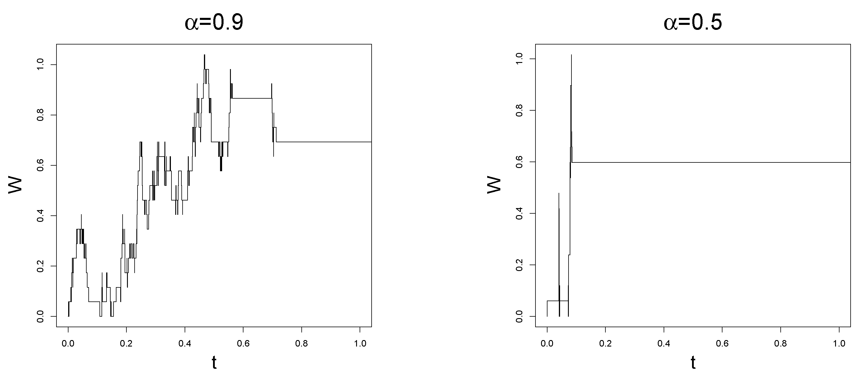
5.2. Simulation of the $\mathrm{DRBM}(\eta ;\alpha )$ with $\eta <0$

Now, we want to use Algorithm 3 to determine a simulation algorithm for the Delayed Reflected Brownian Motion with negative $\eta$. To do this, let us observe that the limit process in Theorem 7 is ${\tilde{Q}}^{\alpha }\sim \mathrm{DRBM}({\lambda }^2\overline{\eta },{\lambda }^3{\overline{\sigma }}^2;\alpha )$ for some constants $\overline{\eta }<0$ and $\overline{\sigma }>0$. Recalling that ${\overline{\sigma }}^2=2/{\lambda }^2$, we know that, in order to have $\mathrm{DRBM}(\eta ,1;\alpha )$, it must hold that $2\lambda =1$, i.e., $\lambda =1/2$, and then $\overline{\eta }=4\eta$. Now, set ${\rho }_n=1-\frac{\zeta }{\sqrt{n}}$, where $\zeta >0$ has to be chosen in a proper way, precisely $\zeta =-\overline{\eta }/2=-2\eta$. However, since we need ${\mu }_n=\frac{n}{2}{\rho }_n^{-1}>0$, it must hold that ${\rho }_n>0$, which is true if and only if $\zeta <\sqrt{n}$. Taking into account this requirement, we can develop an algorithm for the simulation of the DRBM with negative $\eta$ up to time $t_{\mathrm{stop}}>0$ and iteration $n_{\mathrm{it}}>4{\eta }^2$. Again, we only need to simulate the state and calendar arrays of the approximating queue length process and then generate the DRBM from them. This is done in Algorithms 4 and 5.

Algorithm 4 Simulation of a $\mathrm{DRBM}(\eta ;\alpha )$ for $\eta <0$ up to time $t_{\mathrm{stop}}>0$ and iteration $n_{\mathrm{it}}>4{\eta }^2$

procedureSimulateDRBM     ▹ Input: $\eta <0$, $\alpha \in (0,1)$, $t_{\mathrm{stop}}>0$, $n_{\mathrm{it}}>4{\eta }^2$

▹ Output: ${\tilde{W}}_{\alpha }^{\eta }$

$\lambda \leftarrow \frac{n_{\mathrm{it}}}{2}$

$\zeta \leftarrow -2\eta$

$\rho \leftarrow 1-\frac{\zeta }{\sqrt{n_{\mathrm{it}}}}$

$\mu \leftarrow \frac{\lambda }{\rho }$

${\mathcal{X}}_0^{\lambda ,\mu }\leftarrow 0$

${\mathcal{S}}_0^{\lambda ,\mu ,\alpha }\leftarrow 0$

$k\leftarrow 0$

while ${\mathcal{S}}_k^{\lambda ,\mu ,\alpha }<t_{\mathrm{stop}}$ do

$k\leftarrow k+1$

Simulate $\mathcal{U}$ uniform in $(0,1)$

if $\mathcal{U}<p_{\lambda ,\mu }\left({\mathcal{X}}_{k-1}^{\lambda ,\mu }\right)$ then

${\mathcal{X}}_k^{\lambda ,\mu }\leftarrow {\mathcal{X}}_{k-1}^{\lambda ,\mu }+1$

else

${\mathcal{X}}_k^{\lambda ,\mu }\leftarrow {\mathcal{X}}_{k-1}^{\lambda ,\mu }-1$

end if

Simulate $\mathcal{T}\sim \mathrm{Exp}\left(r_{\lambda ,\mu }\left({\mathcal{X}}_{k-1}^{\lambda ,\mu }\right)\right)$

Simulate $S\sim \mathcal{S}\left(\alpha ,1,{cos}^{\frac{1}{\alpha }}\left(\frac{\pi }{2}\alpha \right),0\right)$

${\mathcal{S}}_k^{\lambda ,\mu ,\alpha }\leftarrow {\mathcal{S}}_{k-1}^{\lambda ,\mu ,\alpha }+{\mathcal{T}}^{\frac{1}{\alpha }}S$

end while

${\tilde{W}}_{\alpha }^{\eta }\leftarrow$GenerateDRBM(${\mathcal{X}}^{\lambda ,\mu },{\mathcal{S}}^{\lambda ,\mu ,\alpha },n_{\mathrm{it}}$)

end procedure

Algorithm 5 Generation of the DRBM process from the state and calendar arrays

procedureGenerateDRBM          ▹ Input: ${\mathcal{X}}^{\lambda ,\mu }$, ${\mathcal{S}}^{\lambda ,\mu ,\alpha }$, $n_{\mathrm{it}}$

▹ Output: ${\tilde{W}}_{\alpha }^{\eta }$

function ${\tilde{W}}_{\alpha }^{\eta }$(t)

$\ell \leftarrow \mathrm{length}\left({\mathcal{S}}^{\lambda ,\mu ,\alpha }\right)$           ▹ Recall that the arrays start with 0

$t_{\mathrm{final}}\leftarrow {\mathcal{S}}_{\ell -1}^{\lambda ,\mu ,\alpha }$

if $t_{\mathrm{final}}<t$ then

Error

else

$k\leftarrow 0$

while $t>{\mathcal{S}}_{k+1}^{\lambda ,\mu ,\alpha }$ do

$k\leftarrow k+1$

end while

${\tilde{W}}_{\alpha }^{\eta }\left(t\right)\leftarrow {\mathcal{X}}_k^{\lambda ,\mu }/\sqrt{n_{\mathrm{it}}}$

end if

end function

end procedure

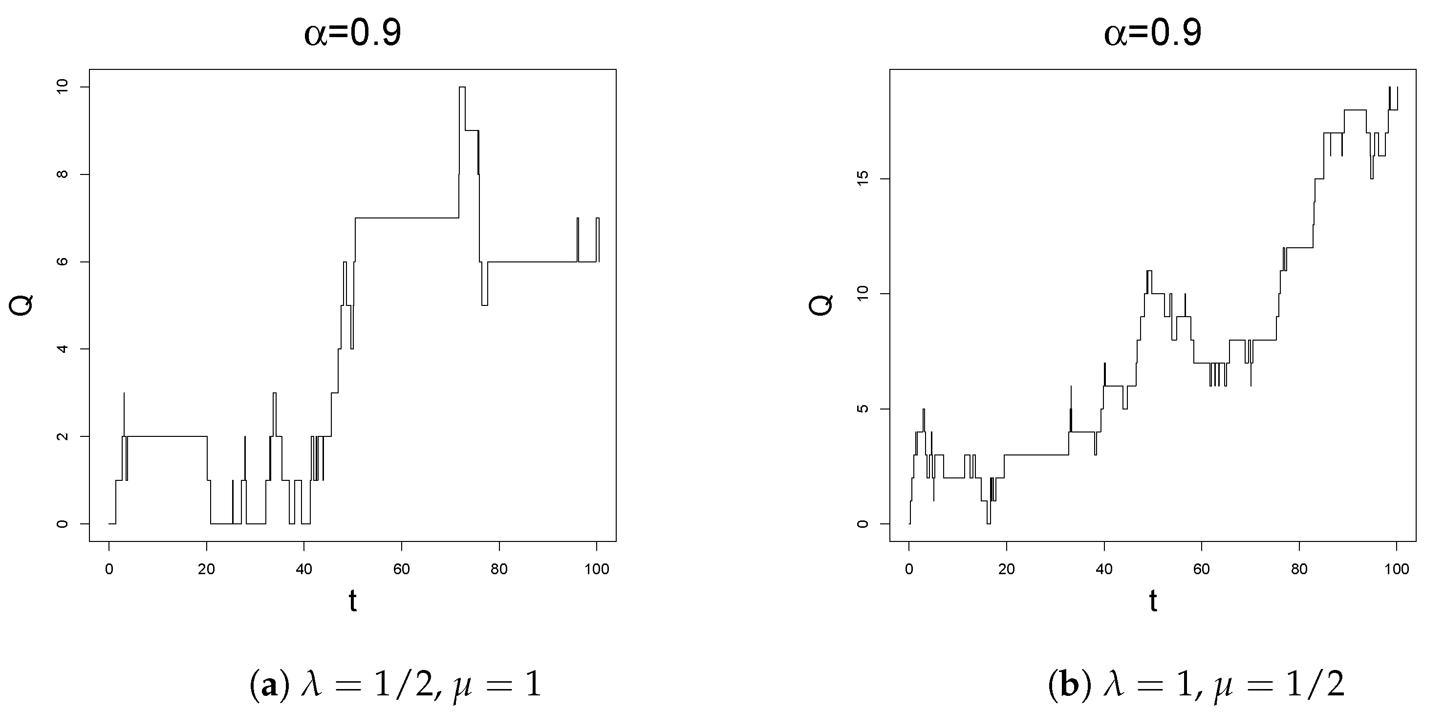
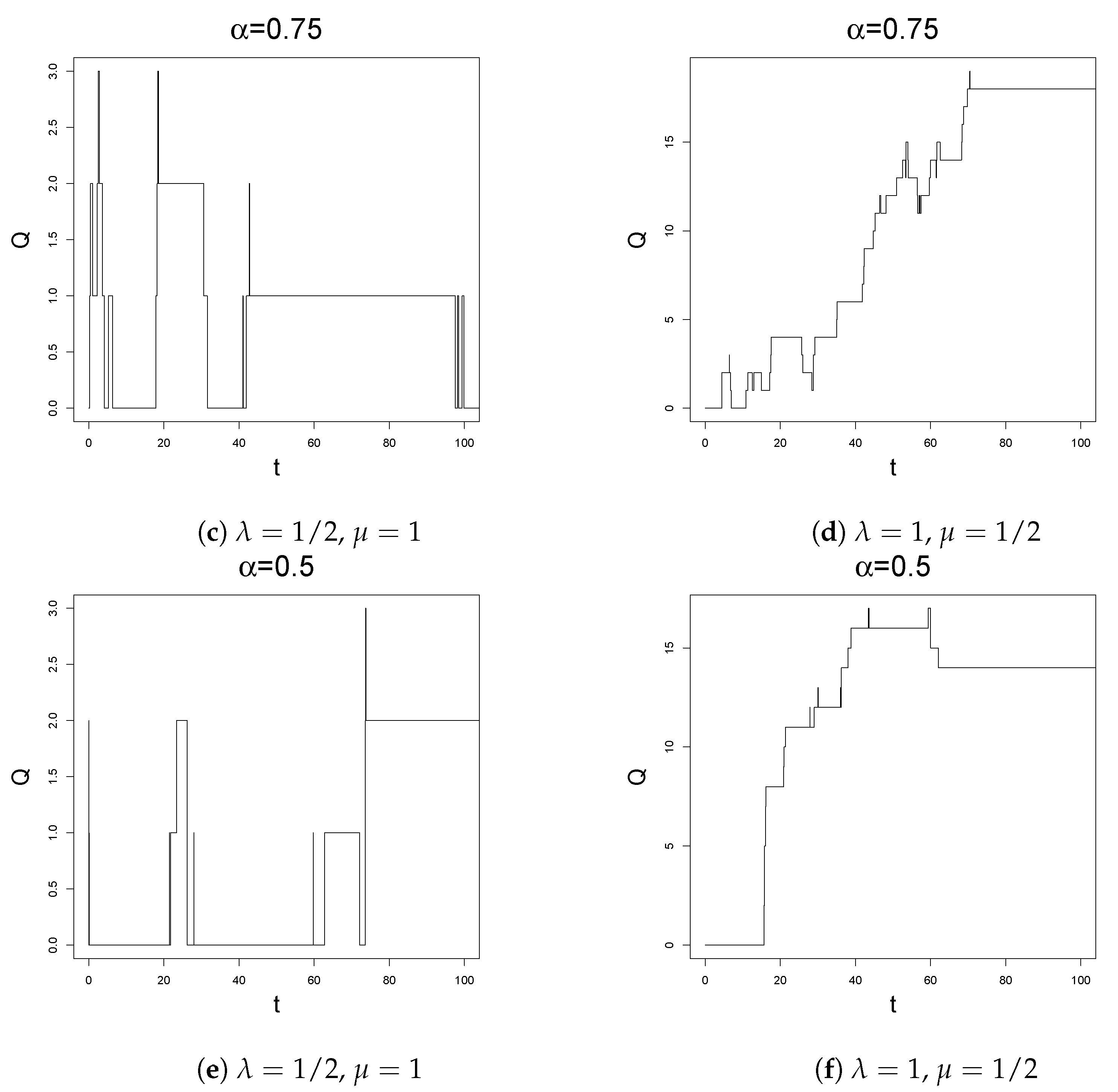
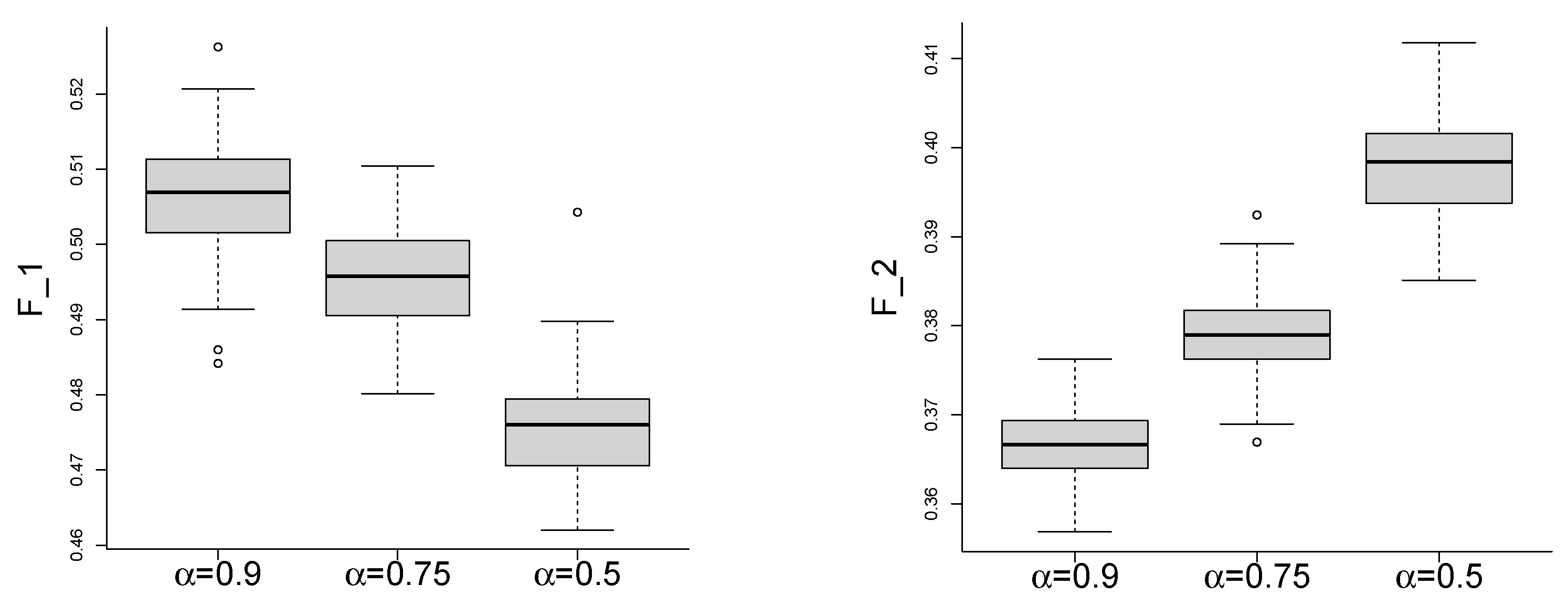
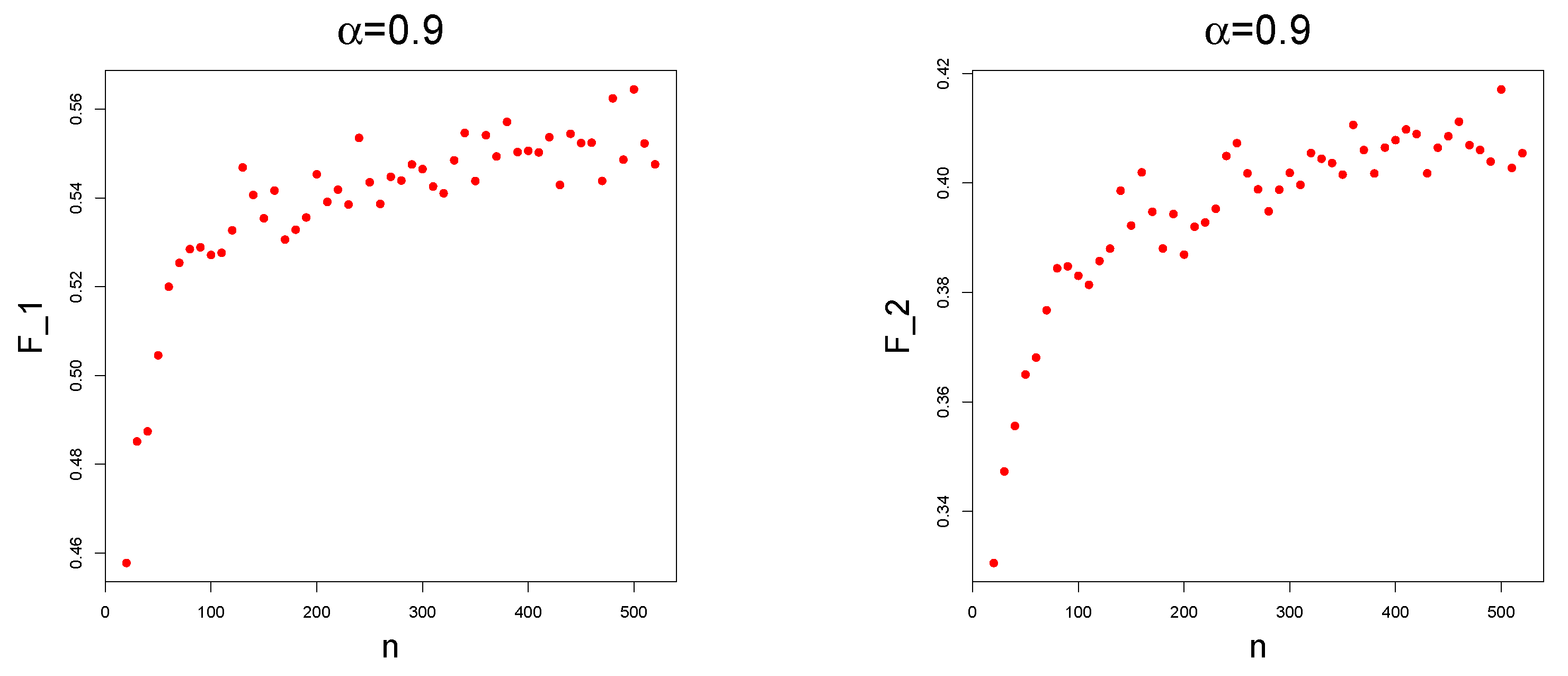
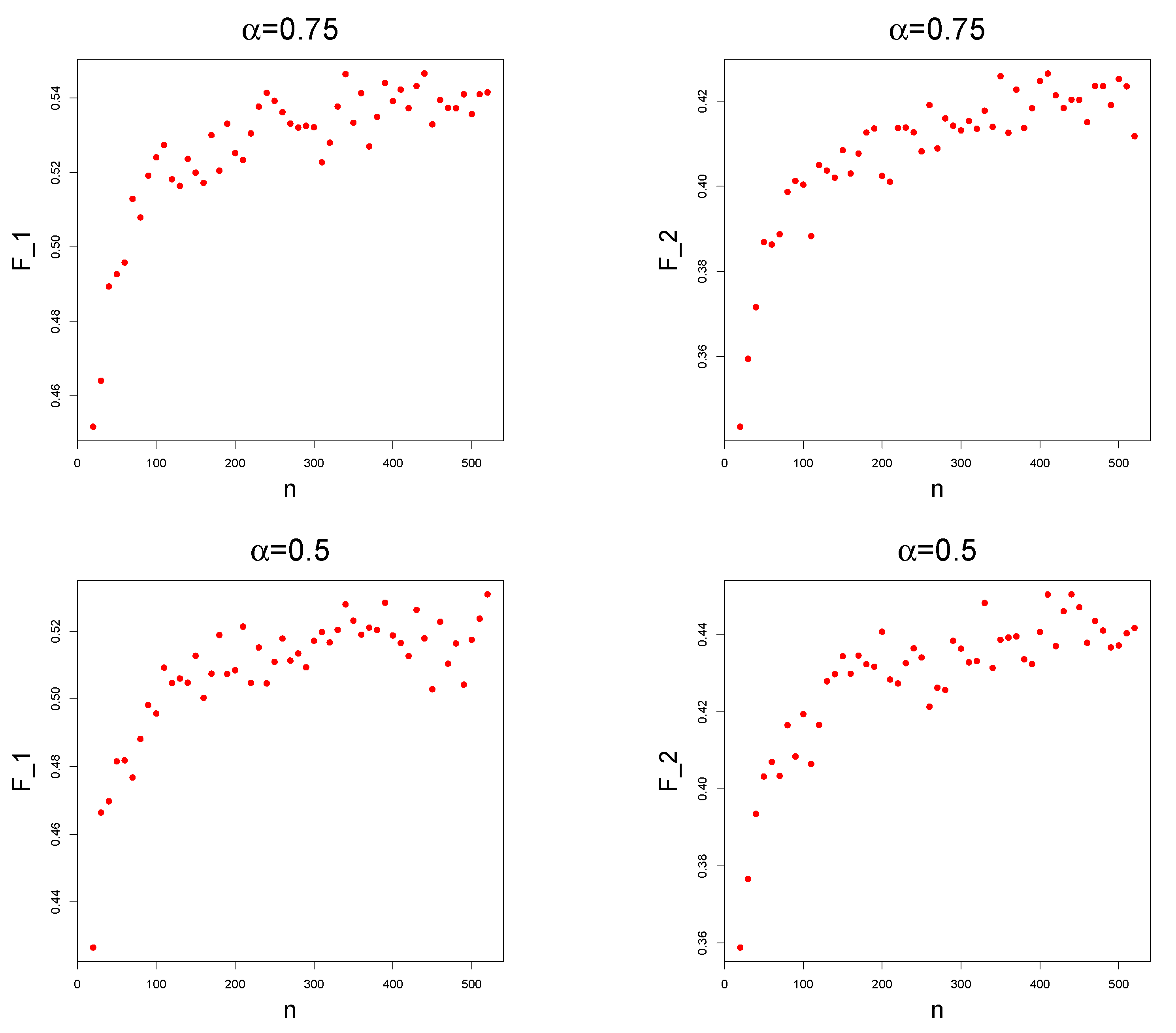
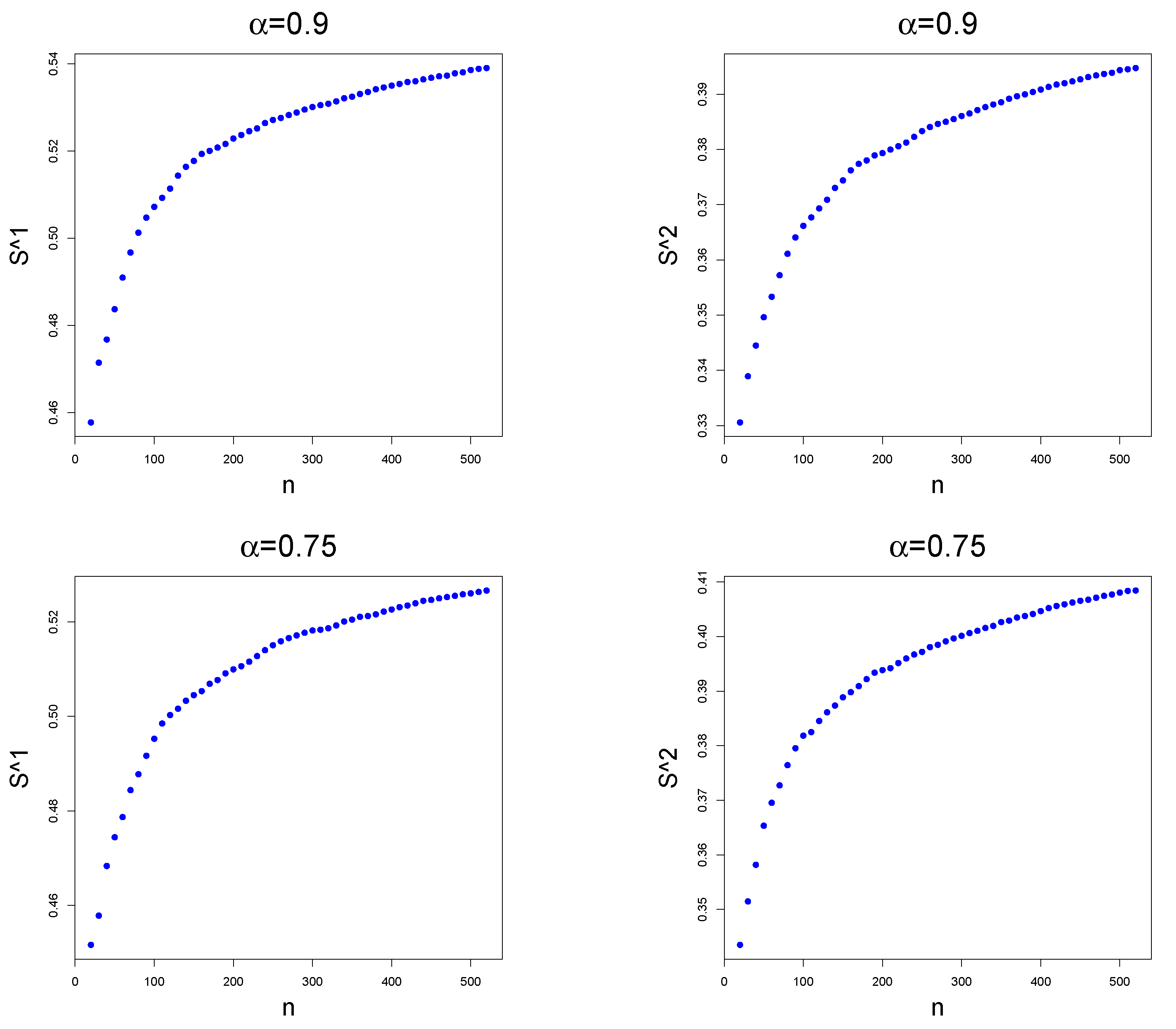
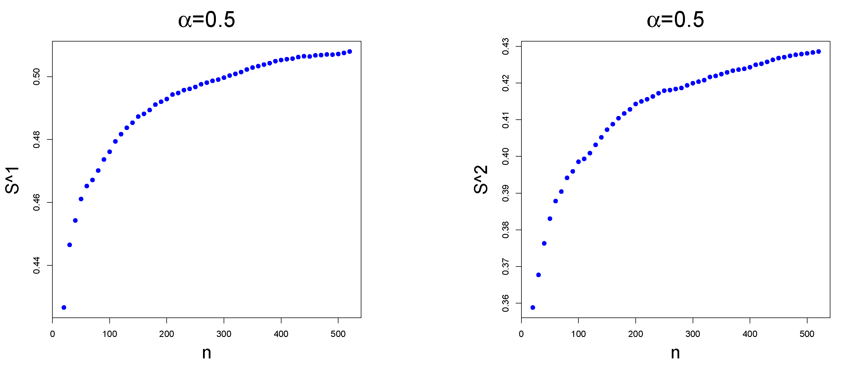
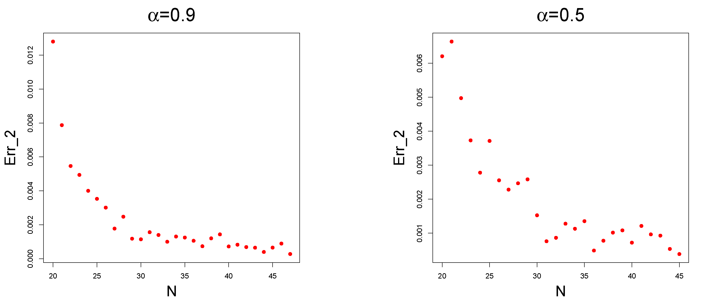
5.3. Numerical Results

In this section, we want to show some simulation results. However, how can one visualize the convergence in distribution?

By the Portmanteau Theorem (see [54] (Chapter 2, Section 3)) and Theorem 7, we know that, for any bounded functional $\mathcal{F}:D\left([0,t_{\mathrm{stop}}]\right)\to \in \mathbb{R}$ that is continuous in the $J_1$ topology, it holds that

$$\underset{n\to +\infty }{lim}\mathbb{E}\left[\mathcal{F}\left(\frac{Q_{\alpha }^{\left(n\right)}}{\sqrt{n}}\right)\right]=\mathbb{E}\left[\mathcal{F}\left({\tilde{W}}_{\alpha }^{\eta }\right)\right]$$

and thus we could study whether

$${\mathbf{e}}_{\mathcal{F}}^{\left(n\right)}:=\left|\mathbb{E}\left[\mathcal{F}\left(\frac{Q_{\alpha }^{\left(n\right)}}{\sqrt{n}}\right)\right]-\mathbb{E}\left[\mathcal{F}\left({\tilde{W}}_{\alpha }^{\eta }\right)\right]\right|$$

converges to 0. However, to do this, we should know $\mathbb{E}\left[\mathcal{F}\left({\tilde{W}}_{\alpha }^{\eta }\right)\right]$ a priori, which is not always possible. Moreover, let us observe that even the evaluation map $x\in D\left([0,t_{\mathrm{stop}}]\right)\mapsto x\left(t\right)\in \mathbb{R}$ is not continuous everywhere in the $J_1$ topology; hence, we need to enlarge the set of possible functionals $\mathcal{F}$. To do this, we need the following weaker version of the Portmanteau Theorem.

Proposition 9.

Let $X_n,X$ be a random variable with values in a metric space $\mathcal{M}$ such that $X_n\Rightarrow X$. Let also $\mathcal{F}:\mathcal{M}\to \mathbb{R}$ be a function such that the following properties hold true:

(i)

It holds that $\mathbb{P}(X\in \mathrm{Disc}(\mathcal{F}\left)\right)=0$;

(ii)

There exist two constants $\epsilon ,M>0$ such that $\mathbb{E}\left[{\left(\mathcal{F}\left(X_n\right)\right)}^{1+\epsilon }\right]\le M$ for any $n\in \mathbb{N}$.

Then,

$$\underset{n\to +\infty }{lim}\mathbb{E}\left[\mathcal{F}\left(X_n\right)\right]=\mathbb{E}\left[\mathcal{F}\left(X\right)\right].$$

Proof. 

By property (i) and the continuous mapping theorem (see [25] (Theorem $\mathrm{3.4.3}$)), we know that $\mathcal{F}\left(X_n\right)\Rightarrow \mathcal{F}\left(X\right)$. Moreover, property (ii) implies that $\mathcal{F}\left(X_n\right)$ are uniformly integrable. We conclude the proof by [54] (Chapter 2, Theorem 3.5).    □

Now, let us select two particular functionals. The first one is given by

$${\mathcal{F}}_1\left(x\right)=x\left(t_{\mathrm{stop}}\right),\forall x\in \mathcal{D}\left([0,t_{\mathrm{stop}}]\right),$$

i.e., it is an evaluation functional. To work with such a functional, we need to prove the following result.

Proposition 10.

The functional ${\mathcal{F}}_1$ satisfies the hypotheses of Proposition 9 with respect to the sequence ${\left(\frac{Q_{\alpha }^{\left(n\right)}}{\sqrt{n}}\right)}_{n\in \mathbb{N}}$.

Proof. 

Let us first observe that if ${\tilde{W}}_{\alpha }^{\eta }$ is continuous, it is clear that $\mathbb{P}({\tilde{W}}_{\alpha }^{\eta }\in \mathrm{Disc}\left({\mathcal{F}}_1\right))=0$; see [25] (Proposition 13.2.1). Thus, we only need to prove item (ii). To do this, let us select $\epsilon =1$ and remark that we need to estimate $n^{-1}\mathbb{E}\left[{\left(Q_{\alpha }^{\left(n\right)}\left(t_{\mathrm{stop}}\right)\right)}^2\right]$. Let $m_{n,\alpha }^{\left(2\right)}\left(t\right)=\mathbb{E}\left[{\left(Q_{\alpha }^{\left(n\right)}\left(t\right)\right)}^2\right]$ and observe that, by a simple conditioning argument,

$$m_{n,\alpha }^{\left(2\right)}\left(t\right)=\mathbb{E}\left[m_{n,1}^{\left(2\right)}\left(L_{\alpha }\left(t\right)\right)\right],$$

where $L_{\alpha }$ is an inverse $\alpha$-stable subordinator independent of $Q_{\alpha }^{\left(n\right)}\left(t\right)$. By [65], we know that $m_{n,1}^{\left(2\right)}$ is increasing. If also $L_{\alpha }$ is almost surely increasing, it is clear that $m_{n,\alpha }^{\left(2\right)}\left(t\right)$ is increasing and then

$$m_{n,\alpha }^{\left(2\right)}\left(t\right)\le \underset{t\to +\infty }{lim}{m}_{n,\alpha }^{\left(2\right)}\left(t\right).$$

Recalling that ${lim}_{t\to +\infty }{L}_{\alpha }\left(t\right)=+\infty$ almost surely, we have, by the monotone convergence theorem,   

$$m_{n,\alpha }^{\left(2\right)}\left(t\right)\le \underset{t\to +\infty }{lim}{m}_{n,1}^{\left(2\right)}\left(t\right).$$

If ${\rho }_n<1$ for any $n\in \mathbb{N}$, we can combine Equations $\left(3.24\right)$ and $\left(3.25\right)$ in [7] to get

$$m_{n,\alpha }^{\left(2\right)}\left(t\right)\le \frac{{\rho }_n(1+{\rho }_n)}{{(1-{\rho }_n)}^2}\le \frac{2n}{{\zeta }^2},$$

where we also use the fact that ${\rho }_n=1-\frac{\zeta }{\sqrt{n}}$. Hence, we finally get

$$\mathbb{E}\left[{\left({\mathcal{F}}_1\left(\frac{Q_{\alpha }^{\left(n\right)}\left(t_{\mathrm{stop}}\right)}{\sqrt{n}}\right)\right)}^2\right]\le \frac{2}{{\zeta }^2}<+\infty ,$$

concluding the proof.    □

The second functional that we consider is the integral functional

$${\mathcal{F}}_2\left(x\right)={\int }_0^{t_{\mathrm{stop}}}x\left(t\right)dt,\forall x\in \mathcal{D}\left([0,t_{\mathrm{stop}}]\right).$$

This time, we will directly prove the limit result.

Proposition 11.

It holds that

$$\underset{n\to +\infty }{lim}\mathbb{E}\left[{\mathcal{F}}_2\left(\frac{Q_{\alpha }^{\left(n\right)}}{\sqrt{n}}\right)\right]=\mathbb{E}\left[{\mathcal{F}}_2\left({\tilde{W}}_{\alpha }^{\eta }\right)\right].$$

Proof. 

Let us first rewrite

$$\mathbb{E}\left[{\mathcal{F}}_2\left(\frac{Q_{\alpha }^{\left(n\right)}}{\sqrt{n}}\right)\right]={\int }_0^{t_{\mathrm{stop}}}\frac{1}{\sqrt{n}}\mathbb{E}\left[Q_{\alpha }^{\left(n\right)}\left(t\right)\right]dt,$$

where we use Fubini’s theorem, being $Q_{\alpha }^{\left(n\right)}\left(t\right)\ge 0$ for all $t\in [0,t_{\mathrm{stop}}]$. By Propositions 9 and 10, we have that

$$\underset{n\to +\infty }{lim}\frac{1}{\sqrt{n}}\mathbb{E}\left[Q_{\alpha }^{\left(n\right)}\left(t\right)\right]=\mathbb{E}\left[{\tilde{W}}_{\alpha }^{\eta }\left(t\right)\right],\forall t\in [0,t_{\mathrm{stop}}].$$

Furthermore, arguing exactly as in the proof of Proposition 10 and using Equation $\left(3.24\right)$ in [7], we get

$$\frac{1}{\sqrt{n}}\mathbb{E}\left[Q_{\alpha }^{\left(n\right)}\left(t\right)\right]\le \frac{1}{\zeta },$$

and thus we can use the dominated convergence theorem to conclude the proof.    □

In particular, $\mathbb{E}\left[{\mathcal{F}}_i\left({\tilde{W}}_{\alpha }^{\eta }\right)\right]$, $i=1,2$, could be estimated numerically by means of Corollary 2 and Mikusinski’s representation of $g_{\alpha }$. However, one still needs to estimate $\mathbb{E}\left[{\mathcal{F}}_i(Q_{\alpha }^{\left(n\right)}/\sqrt{n})\right]$ for $i=1,2$, which is not an easy task since the distribution (and then the expected value) of the fractional $M/M/1$ queue admits some series representations (see [4,21]), which are not easy to evaluate numerically. To overcome this problem, we adopt a Monte Carlo method (with 5000 samples) to determine $\mathbb{E}\left[{\mathcal{F}}_i(Q_{\alpha }^{\left(n\right)}/\sqrt{n})\right]$. However, this means that we have to consider the fact that the evaluated value randomly oscillates around the exact one. For this reason, one cannot use the Cauchy-type error

$${\mathbf{e}}_{\mathcal{F},\mathrm{Cauchy}}^{\left(n\right)}:=\left|\mathbb{E}\left[\mathcal{F}\left(\frac{Q_{\alpha }^{(n+1)}}{\sqrt{n+1}}\right)\right]-\left[\mathcal{F}\left(\frac{Q_{\alpha }^{\left(n\right)}}{\sqrt{n}}\right)\right]\right|$$

to estimate the actual approximation error. In any case, a further investigation on the link between ${\mathbf{e}}_{\mathcal{F},\mathrm{Cauchy}}^{\left(n\right)}$ and ${\mathbf{e}}_{\mathrm{Cauchy}}^{\left(n\right)}$ will be carried out in future works. Let us also underline that, clearly, the oscillation of the Monte Carlo evaluation depends on the variance of ${\mathcal{F}}_i(Q_{\alpha }^{\left(n\right)}/\sqrt{n})$ and, thus, for fixed n, depends on $\alpha$. This is made clear in the boxplots in Figure 2. The plots of $\mathbb{E}\left[{\mathcal{F}}_i(Q_{\alpha }^{\left(n\right)}/\sqrt{n})\right]$ against n are given in Figure 3. The convergence of such a sequence is not so clear due the oscillations caused by the Monte Carlo method. Another visualization of the convergence of $\mathbb{E}\left[{\mathcal{F}}_i(Q_{\alpha }^{\left(n\right)}/\sqrt{n})\right]$ can be obtained by considering the fact that, for any $n_0,\delta \in \mathbb{N}$, the following Cesaro convergence holds:

$$\underset{N\to \infty }{lim}\frac{1}{N}\sum _{n=n_0}^{N+n_0}\mathbb{E}\left[{\mathcal{F}}_i(Q_{\alpha }^{\left(n\delta \right)}/\sqrt{n\delta })\right]=\mathbb{E}\left[{\mathcal{F}}_i\left({\tilde{W}}_{\alpha }^{\eta }\right)\right].$$

Figure 2. Boxplots of 100 simulations of $\mathbb{E}\left[{\mathcal{F}}_i(Q_{\alpha }^{\left(n\right)}/\sqrt{n})\right]$ (resp. $i=1$ on the right and $i=2$ on the left) via Monte Carlo method for $n=50$, $\eta =-1/2$, $t_{\mathrm{stop}}=1$ and different values of $\alpha$.

Figure 3. Point plots of $\mathbb{E}\left[{\mathcal{F}}_i(Q_{\alpha }^{\left(n\right)}/\sqrt{n})\right]$ (resp. $i=1$ on the right and $i=2$ on the left) against n for $\eta =-1/2$, $t_{\mathrm{stop}}=1$ and different values of $\alpha$.

Indeed, the sequence $S_N^{\left(i\right)}:=\frac{1}{N}{\sum }_{n=n_0}^{N+n_0}\mathbb{E}\left[{\mathcal{F}}_i(Q_{\alpha }^{\left(n\delta \right)}/\sqrt{n\delta })\right]$ provides some form of smoothing of the point plot and the convergence is much clearer in this case, as shown in Figure 4. As $S_N^{\left(i\right)}$ is smoother than the original sequence, one could still use the error

$${\tilde{\mathbf{e}}}_{{\mathcal{F}}^i,\mathrm{Cauchy}}^N=|S_{N+1}^{\left(i\right)}-S_N^{\left(i\right)}|$$

to impose a stopping criterion of the form ${\tilde{\mathbf{e}}}_{{\mathcal{F}}^i,\mathrm{Cauchy}}^N<{\epsilon }_{\mathrm{abs}}$ for the absolute error or ${\tilde{\mathbf{e}}}_{{\mathcal{F}}^i,\mathrm{Cauchy}}^N<{\epsilon }_{\mathrm{rel}}{S}_{N+1}^{\left(i\right)}$ for the relative error.

Figure 4. Point plots of $S_N^{\left(i\right)}$ (resp. $i=1$ on the right and $i=2$ on the left) against n for $\eta =-1/2$, $t_{\mathrm{stop}}=1$ and different values of $\alpha$.

With the procedure to simulate the DRBM and $\mathbb{E}\left[\mathcal{F}(Q_{\alpha }^{\left(n\right)}/\sqrt{n})\right]$ is given in Algorithm 6, a simulation algorithm that takes into consideration this stopping criterion is exploited in Algorithm 7. To show some simulated sample paths, we used Algorithm 7 with ${\mathcal{F}}_2$ (which takes into consideration the whole simulated trajectory). The results are illustrated in Figure 5, while the sequence ${\tilde{\mathbf{e}}}_{{\mathcal{F}}^2,\mathrm{Cauchy}}^N$ is plotted in Figure 6.

Algorithm 6 Simulation of $n_{\mathrm{traj}}\in \mathbb{N}$ trajectories of a $\mathrm{DRBM}(\eta ;\alpha )$ for $\eta <0$ up to time $t_{\mathrm{stop}}>0$ with iteration $n>4{\eta }^2$ and evaluation of the functional $\mathbb{E}\left[\mathcal{F}\left({\tilde{W}}_{\alpha }^{\eta }\right)\right]$

procedure SimDRBMwFunc     ▹ Input: $\eta <0$, $\alpha \in (0,1)$, $n,n_{\mathrm{traj}}\in \mathbb{N}$, $n>4{\eta }^2$

▹ Output: ${\left({\mathcal{X}}^{\lambda ,\mu }\right)}_{k,j}$, ${\left({\mathcal{S}}^{\lambda ,\mu ,\alpha }\right)}_{k,j}$, ${\mathcal{F}}_{\mathrm{mean}}$

$\lambda \leftarrow \frac{n}{2}$

$\zeta \leftarrow -2\eta$

$\rho \leftarrow 1-\frac{\zeta }{\sqrt{n}}$

$\mu \leftarrow \frac{\lambda }{\rho }$

${\mathcal{F}}_{\mathrm{mean}}\leftarrow 0$

for $j=1,\cdots ,n_{\mathrm{traj}}$ do

${\mathcal{X}}_{0,j}^{\lambda ,\mu }\leftarrow 0$

${\mathcal{S}}_{0,j}^{\lambda ,\mu ,\alpha }\leftarrow 0$

$k\leftarrow 0$

while ${\mathcal{S}}_{k,j}^{\lambda ,\mu ,\alpha }<t_{\mathrm{stop}}$ do

$k\leftarrow k+1$

Simulate $\mathcal{U}$ uniform in $(0,1)$

if $\mathcal{U}<p_{\lambda ,\mu }\left({\mathcal{X}}_{k-1,j}^{\lambda ,\mu }\right)$ then

${\mathcal{X}}_{k,j}^{\lambda ,\mu }\leftarrow {\mathcal{X}}_{k-1,j}^{\lambda ,\mu }+1$

else

${\mathcal{X}}_{k,j}^{\lambda ,\mu }\leftarrow {\mathcal{X}}_{k-1,j}^{\lambda ,\mu }-1$

end if

Simulate $\mathcal{T}\sim \mathrm{Exp}\left(r_{\lambda ,\mu }\left({\mathcal{X}}_{k-1,j}^{\lambda ,\mu }\right)\right)$

Simulate $S\sim \mathcal{S}\left(\alpha ,1,{cos}^{\frac{1}{\alpha }}\left(\frac{\pi }{2}\alpha \right),0\right)$

${\mathcal{S}}_{k,j}^{\lambda ,\mu ,\alpha }\leftarrow {\mathcal{S}}_{k-1,j}^{\lambda ,\mu ,\alpha }+{\mathcal{T}}^{\frac{1}{\alpha }}S$

end while

${\mathcal{F}}_{\mathrm{mean}}\leftarrow {\mathcal{F}}_{\mathrm{mean}}+{\mathcal{F}}_n({\mathcal{X}}_{·,j}^{\lambda ,\mu },{\mathcal{S}}_{·,j}^{\lambda ,\mu ,\alpha })$

end for

${\mathcal{F}}_{\mathrm{mean}}\leftarrow {\mathcal{F}}_{\mathrm{mean}}/n_{\mathrm{traj}}$

end procedure

Algorithm 7 Simulation of $n_{\mathrm{traj}}\in \mathbb{N}$ trajectories of a $\mathrm{DRBM}(\eta ;\alpha )$ for $\eta <0$ up to time $t_{\mathrm{stop}}>0$ with tolerance ${\epsilon }_{\mathrm{abs}},{\epsilon }_{\mathrm{rel}}>0$ and maximum number of iterations $n_{\max }\in \mathbb{N}$

procedure SimDRBMwTol     ▹ Input: $\alpha \in (0,1)$, $-\eta ,t_{\mathrm{stop}},{\epsilon }_{\mathrm{abs}},{\epsilon }_{\mathrm{rel}}>0$, $n_{\mathrm{traj}},n_{\max },n_0,\delta \in \mathbb{N}$, $n_0>4{\eta }^2$

▹ Output: $n_{\mathrm{traj}}$ trajectories of ${\tilde{W}}_{\alpha }^{\eta }$, ${\mathbf{e}}_{\mathcal{F},\mathrm{Cauchy}}$

$n\leftarrow n_0$

$n_{\mathrm{it}}\leftarrow 0$

${\left({\mathcal{X}}^{\lambda ,\mu }\right)}_{k,j},{\left({\mathcal{S}}^{\lambda ,\mu ,\alpha }\right)}_{k,j},{\mathcal{F}}_{\mathrm{mean}}\leftarrow$SimDRBMwFunc($n,\eta ,\alpha ,n_{\mathrm{traj}}$)

$\widehat{S}\leftarrow {\mathcal{F}}_{\mathrm{mean}}$

$S_0\leftarrow \widehat{S}$

$n\leftarrow n+\delta$

$n_{\mathrm{it}}\leftarrow n_{\mathrm{it}}+1$

${\left({\mathcal{X}}^{\lambda ,\mu }\right)}_{k,j},{\left({\mathcal{S}}^{\lambda ,\mu ,\alpha }\right)}_{k,j},{\mathcal{F}}_{\mathrm{mean}}\leftarrow$SimDRBMwFunc($n,\eta ,\alpha ,n_{\mathrm{traj}}$)

$\widehat{S}\leftarrow \widehat{S}+{\mathcal{F}}_{\mathrm{mean}}$

$S_1\leftarrow \widehat{S}/2$

${\mathbf{e}}_{\mathcal{F},\mathrm{Cauchy}}\leftarrow |S_1-S_0|$

while ${\mathbf{e}}_{\mathcal{F},\mathrm{Cauchy}}\ge min\left\{{\epsilon }_{\mathrm{abs}},{\epsilon }_{\mathrm{rel}}{S}_1\right\}$ and $n_{\mathrm{it}}\le n_{\max }$ do

$n\leftarrow n+\delta$

$n_{\mathrm{it}}\leftarrow n_{\mathrm{it}}+1$

$S_0\leftarrow S_1$

${\left({\mathcal{X}}^{\lambda ,\mu }\right)}_{k,j},{\left({\mathcal{S}}^{\lambda ,\mu ,\alpha }\right)}_{k,j},{\mathcal{F}}_{\mathrm{mean}}\leftarrow$SimDRBMwFunc($n,\eta ,\alpha ,n_{\mathrm{traj}}$)

$\widehat{S}\leftarrow \widehat{S}+{\mathcal{F}}_{\mathrm{mean}}$

$S_1\leftarrow \widehat{S}/(n_{\mathrm{it}}+1)$

${\mathbf{e}}_{\mathcal{F},\mathrm{Cauchy}}\leftarrow |S_1-S_0|$

end while

for $j=1,\cdots ,n_{\mathrm{traj}}$ do

$W_{\alpha ,j}^{\eta }\leftarrow$GenerateDRBM(${\mathcal{X}}_{·,j}^{\lambda ,\mu },{\mathcal{S}}_{·,j}^{\lambda ,\mu ,\alpha },n$)

end for

end procedure

Figure 5. Sample paths of ${\tilde{W}}_{\alpha }^{\eta }$ for $\eta =-1/2$ and different values of $\alpha$ simulated by means of Algorithm 7 with $n_0=20$, $\delta =10$, $n_{\max }=5000$ and ${\epsilon }_{\mathrm{abs}}={\epsilon }_{\mathrm{rel}}=0.001$.

Figure 6. Sequence of ${\tilde{\mathbf{e}}}_{{\mathcal{F}}_2,\mathrm{Cauchy}}^N$ to produce the plots of Figure 5.

6. Conclusions

To summarize the results, we introduced the Delayed Reflected Brownian Motion by means of a suitable time change of the Reflected Brownian Motion (or, equivalently, by solving Skorokhod’s reflection problem on the paths of the Delayed Brownian Motion) and recalled the main properties of fractional $M/M/1$ queues as defined in [4]. These two processes are then linked via the heavy traffic approximation result exploited in Theorem 7. As we also underline in the Introduction, such a theorem can be read in two ways depending on the process that we want to focus on. If we are interested in the properties of the fractional $M/M/1$ queues, the theorem provides a subdiffusive approximation of them, in terms of the Delayed Reflected Brownian Motion, as the traffic intensity $\rho$ is near 1. This is quite useful if one needs to investigate (approximatively) some distributional property of a fractional $M/M/1$ queue in the transient state. Indeed, different formulations of the one-dimensional distribution of the queue length process in the fractional case are given in [4,21] but they involve nested series of functions, which can be difficult to evaluate even numerically. However, if $\rho$ is near 1, one can approximate the one-dimensional distribution of the queue length process with the one of the Delayed Reflected Brownian Motion given in Proposition 5, which can be numerically evaluated thanks to Mikusinski’s representation of the density of the stable subordinator.

Vice versa, if we are interested in the properties of the Delayed Reflected Brownian Motion, Theorem 7 provides a continuous-time random walk approximation of such a process. This is a quite useful property when combined with the discrete event simulation procedure (which is a generalization of the well-known Gillespie’s algorithm; see [31,63]). Indeed, the simulation of an inverse $\alpha$-stable subordinator is usually done by means of Laplace inversion, if we start from the Laplace transform of $f_{\alpha }$, or by inverting the subordinator, which is instead simulated via the Chambers–Mallow–Stuck method [55]. The algorithm presented in the paper does not rely at all on the simulation of the inverse subordinator, thanks to the fact that we are able to simulate Mittag–Leffler random variables by using the Chambers–Mallow–Stuck method.

This second point of view is investigated with more attention in Section 5. Precisely, Theorem 7 gives us a limit result, but does not tell us how large we should chose n to have a suitably good approximation. Moreover, as we observed before, estimating the distributional properties of a fractional queue is not an easy task, due to the quite complicated form of the state probabilities. However, some distributional quantities can be provided by Monte Carlo estimates, which, due to the random nature of the approach, invalidates the idea of using a form of error based on the Cauchy property of converging sequences. This problem can be overcome by using the Cesaro convergence of the sequence, as taking the average smooths in some sense the oscillating simulated data, as one can observe by comparing Figure 3 and Figure 4. Thus, one can use the sequence of averages in place of the original one to provide a stopping criterion, as done in Algorithm 7. Such an approach is supported by the sequence of errors given in Figure 6. Clearly, one could use other smoothing procedures on data to overcome the oscillations caused by Monte Carlo estimates. In future works, we aim to discuss the properties of time-changed $M/M/1$ queues and Reflected Brownian Motions with more general inverse subordinators, trying to link them via a heavy traffic approximation result. The simulation of such types of queueing models will require some more sophisticated methods, due to the lack, in general, of both the self-similarity property and a special algorithm for the subordinator.

References

- Erlang, A.K. The theory of probabilities and telephone conversations. Nyt. Tidsskr. Mat. Ser. B 1909, 20, 33–39. [Google Scholar]
- Helbing, D. A section-based queueing-theoretical traffic model for congestion and travel time analysis in networks. J. Phys. A Math. Gen. 2003, 36, L593. [Google Scholar] [CrossRef]
- Kleinrock, L. Queueing Systems: Computer Applications; John Wiley: Hoboken, NJ, USA, 1976. [Google Scholar]
- Cahoy, D.O.; Polito, F.; Phoha, V. Transient behavior of fractional queues and related processes. Methodol. Comput. Appl. Probab. 2015, 17, 739–759. [Google Scholar] [CrossRef]
- Schoutens, W. Stochastic Processes and Orthogonal Polynomials; Springer Science & Business Media: Berlin/Heidelberg, Germany, 2012; Volume 146. [Google Scholar]
- Ross, S.M. Introduction to Probability Models; Academic Press: Cambridge, MA, USA, 2014. [Google Scholar]
- Kleinrock, L. Queueing Systems: Theory; John Wiley: Hoboken, NJ, USA, 1975. [Google Scholar]
- Conolly, B.; Langaris, C. On a new formula for the transient state probabilities for M/M/1 queues and computational implications. J. Appl. Probab. 1993, 30, 237–246. [Google Scholar] [CrossRef]
- Parthasarathy, P. A transient solution to an M/M/1 queue: A simple approach. Adv. Appl. Probab. 1987, 19, 997–998. [Google Scholar] [CrossRef]
- Levy, P. Processus semi-markoviens. In Proceedings of the International Congress of Mathematicians, Amsterdam, The Netherlands, 2–9 September 1954. [Google Scholar]
- Orsingher, E.; Polito, F. Fractional pure birth processes. Bernoulli 2010, 16, 858–881. [Google Scholar] [CrossRef]
- Orsingher, E.; Polito, F. On a fractional linear birth–death process. Bernoulli 2011, 17, 114–137. [Google Scholar] [CrossRef]
- Leonenko, N.N.; Meerschaert, M.M.; Sikorskii, A. Fractional Pearson diffusions. J. Math. Anal. Appl. 2013, 403, 532–546. [Google Scholar] [CrossRef]
- Ascione, G.; Leonenko, N.; Pirozzi, E. Fractional immigration-death processes. J. Math. Anal. Appl. 2021, 495, 124768. [Google Scholar] [CrossRef]
- Laskin, N. Fractional Poisson process. Commun. Nonlinear Sci. Numer. Simul. 2003, 8, 201–213. [Google Scholar] [CrossRef]
- Meerschaert, M.; Nane, E.; Vellaisamy, P. The fractional Poisson process and the inverse stable subordinator. Electron. J. Probab. 2011, 16, 1600–1620. [Google Scholar] [CrossRef]
- Baeumer, B.; Meerschaert, M.M. Stochastic solutions for fractional Cauchy problems. Fract. Calc. Appl. Anal. 2001, 4, 481–500. [Google Scholar]
- Scalas, E.; Toaldo, B. Limit theorems for prices of options written on semi-Markov processes. Theory Probab. Math. Stat. 2021, 105, 3–33. [Google Scholar] [CrossRef]
- Ascione, G.; Cuomo, S. A sojourn-based approach to semi-Markov Reinforcement Learning. arXiv 2022, arXiv:2201.06827. [Google Scholar]
- Ascione, G.; Toaldo, B. A semi-Markov leaky integrate-and-fire model. Mathematics 2019, 7, 1022. [Google Scholar] [CrossRef]
- Ascione, G.; Leonenko, N.; Pirozzi, E. Fractional queues with catastrophes and their transient behaviour. Mathematics 2018, 6, 159. [Google Scholar] [CrossRef]
- De Oliveira Souza, M.; Rodriguez, P.M. On a fractional queueing model with catastrophes. Appl. Math. Comput. 2021, 410, 126468. [Google Scholar]
- Ascione, G.; Leonenko, N.; Pirozzi, E. Fractional Erlang queues. Stoch. Process. Their Appl. 2020, 130, 3249–3276. [Google Scholar] [CrossRef]
- Ascione, G.; Leonenko, N.; Pirozzi, E. On the Transient Behaviour of Fractional M/M/∞ Queues. In Nonlocal and Fractional Operators; Springer: Berlin/Heidelberg, Germany, 2021; pp. 1–22. [Google Scholar]
- Whitt, W. Stochastic-Process Limits: An Introduction to Stochastic-Process Limits and their Application to Queues; Springer Science & Business Media: Berlin/Heidelberg, Germany, 2002. [Google Scholar]
- Skorokhod, A.V. Stochastic equations for diffusion processes in a bounded region. II. Theory Probab. Its Appl. 1962, 7, 3–23. [Google Scholar] [CrossRef]
- Magdziarz, M.; Schilling, R. Asymptotic properties of Brownian motion delayed by inverse subordinators. Proc. Am. Math. Soc. 2015, 143, 4485–4501. [Google Scholar] [CrossRef]
- Capitanelli, R.; D’Ovidio, M. Delayed and rushed motions through time change. Lat. Am. J. Probab. Math. Stat. 2020, 17, 183–204. [Google Scholar] [CrossRef]
- Graversen, S.E.; Shiryaev, A.N. An extension of P. Lévy’s distributional properties to the case of a Brownian motion with drift. Bernoulli 2000, 6, 615–620. [Google Scholar] [CrossRef]
- Kobayashi, K. Stochastic calculus for a time-changed semimartingale and the associated stochastic differential equations. J. Theor. Probab. 2011, 24, 789–820. [Google Scholar] [CrossRef]
- Asmussen, S.; Glynn, P.W. Stochastic Simulation: Algorithms and Analysis; Springer Science & Business Media: Berlin/Heidelberg, Germany, 2007; Volume 57. [Google Scholar]
- Ambrosio, L.; Fusco, N.; Pallara, D. Functions of Bounded Variation and Free Discontinuity Problems; Courier Corporation: Washington, DC, USA, 2000. [Google Scholar]
- Dupuis, P.; Ramanan, K. Convex duality and the Skorokhod problem. I. Probab. Theory Relat. Fields 1999, 115, 153–195. [Google Scholar] [CrossRef]
- Harrison, J.M. Brownian Motion and Stochastic Flow Systems; Wiley: New York, NY, USA, 1985. [Google Scholar]
- Abate, J.; Whitt, W. Transient behavior of regulated Brownian motion, I: Starting at the origin. Adv. Appl. Probab. 1987, 19, 560–598. [Google Scholar] [CrossRef]
- Kinkladze, G. A note on the structure of processes the measure of which is absolutely continuous with respect to the Wiener process modulus measure. Stochastics: Int. J. Probab. Stoch. Process. 1982, 8, 39–44. [Google Scholar] [CrossRef]
- Revuz, D.; Yor, M. Continuous Martingales and Brownian Motion; Springer Science & Business Media: Berlin/Heidelberg, Germany, 2013; Volume 293. [Google Scholar]
- Göttlich, S.; Lux, K.; Neuenkirch, A. The Euler scheme for stochastic differential equations with discontinuous drift coefficient: A numerical study of the convergence rate. Adv. Differ. Equ. 2019, 2019, 429. [Google Scholar] [CrossRef]
- Asmussen, S.; Glynn, P.; Pitman, J. Discretization error in simulation of one-dimensional reflecting Brownian motion. Ann. Appl. Probab. 1995, 5, 875–896. [Google Scholar] [CrossRef]
- Buonocore, A.; Nobile, A.G.; Pirozzi, E. Simulation of sample paths for Gauss-Markov processes in the presence of a reflecting boundary. Cogent Math. 2017, 4, 1354469. [Google Scholar] [CrossRef]
- Buonocore, A.; Nobile, A.G.; Pirozzi, E. Generating random variates from PDF of Gauss–Markov processes with a reflecting boundary. Comput. Stat. Data Anal. 2018, 118, 40–53. [Google Scholar] [CrossRef]
- Bertoin, J. Subordinators: Examples and Applications. In Lectures on Probability Theory and Statistics; Springer: Berlin/Heidelberg, Germany, 1999; pp. 1–91. [Google Scholar]
- Meerschaert, M.M.; Sikorskii, A. Stochastic Models for Fractional Calculus; de Gruyter: Berlin, Germany, 2019. [Google Scholar]
- Meerschaert, M.M.; Straka, P. Inverse stable subordinators. Math. Model. Nat. Phenom. 2013, 8, 1–16. [Google Scholar] [CrossRef] [PubMed]
- Arendt, W.; Batty, C.J.; Hieber, M.; Neubrander, F. Vector-Valued Laplace Transforms and Cauchy Problems; Springer: Berlin/Heidelberg, Germany, 2011. [Google Scholar]
- Mikusiński, J. On the function whose Laplace-transform is e-sα. Stud. Math. 1959, 2, 191–198. [Google Scholar] [CrossRef]
- Saa, A.; Venegeroles, R. Alternative numerical computation of one-sided Lévy and Mittag-Leffler distributions. Phys. Rev. E 2011, 84, 026702. [Google Scholar] [CrossRef] [PubMed]
- Penson, K.; Górska, K. Exact and explicit probability densities for one-sided Lévy stable distributions. Phys. Rev. Lett. 2010, 105, 210604. [Google Scholar] [CrossRef]
- Ascione, G.; Patie, P.; Toaldo, B. Non-local heat equation with moving boundary and curve-crossing of delayed Brownian motion. 2022; in preparation. [Google Scholar]
- Leonenko, N.; Pirozzi, E. First passage times for some classes of fractional time-changed diffusions. Stoch. Anal. Appl. 2021, 1–29. [Google Scholar] [CrossRef]
- Meerschaert, M.M.; Straka, P. Semi-Markov approach to continuous time random walk limit processes. Ann. Probab. 2014, 42, 1699–1723. [Google Scholar] [CrossRef][Green Version]
- Çinlar, E. Markov additive processes. II. Z. Wahrscheinlichkeitstheorie Verwandte Geb. 1972, 24, 95–121. [Google Scholar] [CrossRef]
- Kaspi, H.; Maisonneuve, B. Regenerative systems on the real line. Ann. Probab. 1988, 16, 1306–1332. [Google Scholar] [CrossRef]
- Billingsley, P. Convergence of Probability Measures; John Wiley & Sons: Hoboken, NJ, USA, 2013. [Google Scholar]
- Chambers, J.M.; Mallows, C.L.; Stuck, B. A method for simulating stable random variables. J. Am. Stat. Assoc. 1976, 71, 340–344. [Google Scholar] [CrossRef]
- Borovkov, A. Some limit theorems in the theory of mass service. Theory Probab. Its Appl. 1964, 9, 550–565. [Google Scholar] [CrossRef]
- Iglehart, D.L.; Whitt, W. Multiple channel queues in heavy traffic. I. Adv. Appl. Probab. 1970, 2, 150–177. [Google Scholar] [CrossRef]
- Kilbas, A.A.; Srivastava, H.M.; Trujillo, J.J. Theory and Applications of Fractional Differential Equations; Elsevier: Amsterdam, The Netherlands, 2006; Volume 204. [Google Scholar]
- Mainardi, F.; Gorenflo, R.; Scalas, E. A fractional generalization of the Poisson processes. Vietnam J. Math. 2004, 32, 53–64. [Google Scholar]
- Mainardi, F.; Gorenflo, R.; Vivoli, A. Renewal processes of Mittag-Leffler and Wright type. Fract. Calc. Appl. Anal. 2005, 8, 7–38. [Google Scholar]
- Bingham, N.H. Limit theorems for occupation times of Markov processes. Z. Wahrscheinlichkeitstheorie Verwandte Geb. 1971, 17, 1–22. [Google Scholar] [CrossRef]
- Peng, J.; Li, K. A note on property of the Mittag-Leffler function. J. Math. Anal. Appl. 2010, 370, 635–638. [Google Scholar] [CrossRef]
- Gillespie, D.T. A general method for numerically simulating the stochastic time evolution of coupled chemical reactions. J. Comput. Phys. 1976, 22, 403–434. [Google Scholar] [CrossRef]
- Nolan, J.P. Numerical calculation of stable densities and distribution functions. Commun. Statistics Stoch. Model. 1997, 13, 759–774. [Google Scholar] [CrossRef]
- Abate, J.; Whitt, W. Transient behavior of the M/M/l queue: Starting at the origin. Queueing Syst. 1987, 2, 41–65. [Google Scholar] [CrossRef]
Publisher’s Note: MDPI stays neutral with regard to jurisdictional claims in published maps and institutional affiliations. |
© 2022 by the authors. Licensee MDPI, Basel, Switzerland. This article is an open access article distributed under the terms and conditions of the Creative Commons Attribution (CC BY) license (https://creativecommons.org/licenses/by/4.0/).