Intermittency Reinjection in the Logistic Map

Abstract

Just below a Period-3 window, the logistic map exhibits intermittency. Then, the third iterate of this map has been widely used to explain the chaotic intermittency concept. Much attention has been paid to describing the behavior around the vanished fixed points, the tangent bifurcation, and the formation of the characteristic channel between the map and the diagonal for type-I intermittency. However, the reinjection mechanism has not been deeply analyzed. In this paper, we studied the reinjection processes for the three fixed points around which intermittency is generated. We calculated the reinjection probability density function, the probability density of the laminar lengths, and the characteristic relation. We found that the reinjection mechanisms have broader behavior than the usually used uniform reinjection. Furthermore, the reinjection processes depend on the fixed point.

1. Introduction

Intermittency is a route by which a dynamical system evolves from regular behavior to chaos. In chaotic intermittency, a dynamical system alternates laminar phases with chaotic bursts. The laminar or regular behaviors correspond to pseudo-equilibrium or pseudo-periodic solutions, while the bursts are related to chaotic evolution [1,2,3].

Several processes and mechanisms display chaotic intermittency. It has been found in physical, chemical, medical, and economic phenomena, among others [4,5,6,7,8,9,10,11,12,13,14]. A more complete description of chaotic intermittency could help in the correct understanding of these phenomena.

At the end of the 1940s, the word intermittency was employed in turbulent flows [15]. Approximately thirty years later, chaotic intermittency was classified into three types named I, II, and III [16]. This categorization follows the periodic orbit stability loss using the system Floquet multipliers or the fixed-point loss of stability in a map taking the map’s eigenvalues. Type-I intermittency occurs when an eigenvalue moves away from the unit circle across +1 and a tangent bifurcation occurs. Type-II intermittency happens when two complex-conjugate eigenvalues escape from the unit circle by a Hopf bifurcation. Finally, type III occurs by a subcritical period-doubling bifurcation when an eigenvalue goes out of the unit circle by −1 [2,3].

Subsequent studies found other types of intermittency, such as V, X, on–off, eyelet, ring, etc. References [17,18,19] introduced the concept of intermittency type V. This takes place if a stable fixed point in a non-differentiable, even discontinuous, map impacts with a non-differentiable or discontinuous point. Price and Mullin, in 1991, introduced the type X intermittency concept [20]. It is similar to type-I intermittency. Both intermittencies have the same local map. However, they are distinct, each one having specific characteristics. Type X intermittency possesses a regular reinjection process and a hysteresis mechanism. Intermittency type on–off is depicted by sudden alterations between approximately constant periods or static states and irregular bursts. The static states are the “off” states, while the bursts correspond to “on” states, which leave and return suddenly to the “off” states [21,22]. The simplest on–off intermittency has two components: an invariant object and trajectories in and out of each small neighborhood of the invariant object. Eyelet intermittency was discovered at the border of the phase synchronization of coupled oscillators. The occurrence of eyelet intermittency is depicted using the synchronization of the unstable periodic saddle orbits embedded in chaotic attractors [23,24,25]. The eyelet intermittency concept was introduced by the analysis of the start of the phase synchronization. Another intermittent behavior, known as ring intermittency, also takes place close to the phase synchronization region boundary. Nevertheless, this intermittency happens for high initial frequency mismatches for two coupled systems [26].

For one-dimensional maps, chaotic intermittency is generated by a local map and a mechanism of reinjection [1,2,3]. The local map determines the intermittency type, and the reinjection process drives the trajectories’ return from the chaotic behavior to the laminar zone. The reinjection probability density function (RPD function) is utilized to specify the probability that trajectories are reinjected in the laminar interval [1,2,3]. The accurate description of the RPD function is fundamental to correctly calculate the chaotic intermittency. There was not a theory to describe the RPD function, and different schemes were implemented, the uniform RPD function being the most used [1,2,16,27]. In recent years, a more general scheme, called the M function methodology, was introduced [3]. It has accurately worked for maps showing type-I, -II, -III, and -V intermittencies with and without noise [28,29,30,31]. Furthermore, the RPD function depends on the map derivative at pre-reinjection points [32]. If the pre-reinjection points are extreme or point with an infinite derivative, the RPD function is not uniform [3].

Chaotic intermittency and its applications are current research topics [33,34,35]. Furthermore, studies about intermittency and the logistic map have been recently published [36,37]. The logistic map, $L_{\mu }\left(x\right)$, exhibits intermittency just below a Period-3 window. Then, the third iterate, $L_{\mu }^3\left(x\right)$, has been widely used to explain chaotic intermittency [1,2,38,39]. However, very little attention has been given to describe the reinjection processes, which show different behaviors depending on the fixed point of the map. In this paper, we studied the reinjection processes in type-I intermittency for the third iterate of the logistic map. To develop this task, we used recent advances in chaotic intermittency. In addition, we calculated the following statistical variables: the laminar length, the probability density of the laminar lengths, and the characteristic relation.

For $\mu <{\mu }_c=1+\sqrt{8}$, type-I intermittency occurs around three fixed points $x_{01}\cong 0.15992881844625645$, $x_{02}\cong 0.5143552770619905$, and $x_{03}\cong 0.9563178419736238$. By the map symmetry, the reinjection process is different for $x_{01}$ and $x_{03}$ concerning $x_{02}$. The main objective is to show that the reinjection process is more complex than described in previous studies and to introduce a work methodology to evaluate the main statistical variables of chaotic intermittency.

2. The Logistic Map

The logistic map has been widely studied [1,2,38,39,40]. It is a discrete analog of the logistic equation introduced to study population evolution [38,40]. It can be written as:

$$L_{\mu }\left(x\right)=\mu x(1-x),$$

(1)

where $\mu$ is a positive real parameter and x is a dimensionless measure of the population, $0\le x\le 1$. The maximum of $L_{\mu }$ is $\mu /4$, which is obtained at $x=1/2$. For $0<\mu \le 4$, the logistic equation maps the interval $[0,1]$ into itself.

Because $L_{\mu }\left(x\right)$ shows intermittency just below a Period-3 window, we studied the third iterate map of Equation (1):

$$x_{n+1}=L_{\mu }\left(L_{\mu }\left(L_{\mu }\left(x_n\right)\right)\right))=L_{\mu }^3\left(x_n\right).$$

(2)

We describe the behavior of the Period-3 cycle of Equation (1) as the parameter $\mu$ decreases from slightly above the critical value ${\mu }_c=1+\sqrt{8}$ to slightly below it. For $\mu =1+\sqrt{8}+0.002$, the logistic map has a stable Period-3 cycle consisting of the following points: $0.1556...,0.5034...,0.9575...$ [39]. If we consider ${\mu }_c=1+\sqrt{8}$, the map $L_{\mu }^3\left(x\right)-x$ has three double roots, which are at $x_{01}=0.15992881844625645...$, $x_{02}=0.5143552770619905...$, and $x_{03}=0.9563178419736238...$. At these points, $\frac{d{L}_{\mu }^3}{dx}=1$, and the graph of $L_{\mu }^3$ is tangent to the diagonal. Note that the eighth-degree polynomial $L_{\mu }^3\left(x\right)-x$ has additional roots, which correspond to unstable fixed points. For $\mu <1+\sqrt{8}$, but close it, type-I intermittency occurs by a tangent bifurcation. The laminar intervals are placed around the vanished fixed points $x_{01},x_{02},x_{03}$. However, the reinjection processes around these points are different and depend on the fixed point. We studied the reinjection mechanism for these points using recent advances to analyze chaotic intermittency [3,28,31,41,42].

3. Intermittency in the Logistic Map: Reinjection Processes

There are fixed-point theorems that determine the existence of fixed points in maps [39,43,44,45]. As we explained in Section 2, the map $L_{\mu }^3\left(x\right)$ for ${\mu }_c$ has three fixed points in which type-I intermittency occurs $x_{01}=0.15992881844625645...$, $x_{02}=0.5143552770619905...$, and $x_{03}=0.9563178419736238...$. However, the reinjection processes are different for $x_{01}$ than that for $x_{02}$.

To understand the reinjection mechanisms, we have to describe the pre-reinjection points for the map $L_{\mu }^3\left(x\right)$. The pre-reinjection points are the $x_{n-1}$ points for which $x_n=L_{\mu }^3\left(x_{n-1}\right)$, where $x_n$ points are inside the laminar interval and $x_{n-1}$ outside the laminar interval. The pre-reinjection points govern (have a strong influence on) the reinjection process [3].

The derivative of the map at pre-reinjection points is different for $x_{01}$ and $x_{03}$ than that for $x_{02}$. Furthermore, the pre-reinjection points depend on the length of the laminar interval. Therefore, the reinjection mechanism and the statistical variables depend on the fixed point.

3.1. Fixed Point $x_{01}$: Non-Uniform RPD Function

First, we studied the intermittency phenomenon for the fixed point $x_{01}$. With no loss of generality, we move the map $L_{\mu }^3\left(x\right)$, so the fixed point $x_{01}$ coincides with the origin of the coordinate system. Accordingly, the map results in:

$$\begin{array}{cc}F\left(x\right)=\hfill & -x_{01}+{\mu }^3(1-(x+x_{01}))(x+x_{01})(1+\mu (-1+(x+x_{01}))(x+x_{01}))\hfill \\ \\ \hfill & \times (1+{\mu }^2(-1+(x+x_{01}))(x+x_{01})(1+\mu (-1+(x+x_{01}))(x+x_{01}))).\hfill \end{array}$$

(3)

Figure 1 displays this map (blue line) and the pre-reinjection points (red points) for $c=0.04(I_l=[-0.04,0.04])$ and $\mu =3.828$.

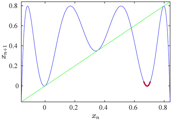
Figure 1. Map given by Equation (3) and pre-reinjection points for $x_{01}$, $c=0.04$, and $\mu =3.828$. Blue line: map. Red points: pre-reinjection points. Green line: bisector.

To calculate the RPD function, we utilized the M function methodology described in Appendix B. The numerical data are generated by an iterative process for the map given by Equation (3). The laminar interval is divided into $N_s$ sub-intervals; subsequently, the histogram of reinjections and the numerical RPD function are calculated. To evaluate the histogram, at least $100N_s$ reinjections were considered. On the other hand, the theoretical RPD function can be written as (see Appendix A and Appendix B):

$$\varphi \left(x\right)=b{(x-\widehat{x})}^{\alpha },\alpha =\frac{2m-1}{1-m}.$$

(4)

We carried out several numerical tests evaluating the RPD functions using the M function methodology. For $c=0.01$, $\mu =3.828$, N = 100,000, and $N_s=500$, the exponent of the RPD function results in $\alpha =-0.483550438$ ($m=0.340564945$), and the lower boundary of reinjection $\widehat{x}=-0.00240279$. For $c=0.04$, $\mu =3.8284$, N = 100,000 and $N_s=1000$, we obtained $\alpha =-0.494355923$ and $\widehat{x}=-0.00273628$. Figure 2 shows the numerical and theoretical RPD functions for both tests. The blue lines and the red points are the theoretical and numerical RPDs, respectively. From the figure, we note a high accuracy between the theoretical and numerical results.

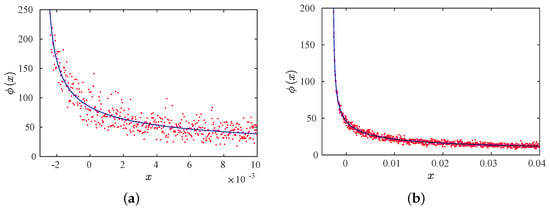
Figure 2. Theoretical and numerical RPDs for $\mu =3.828$. (a) $c=0.01$, $N_s=500$. (b) $c=0.04$, $N_s=1000$. Blue lines: theoretical RPDs. Red points: numerical RPDs.

Furthermore, we used $\mu =3.8275,3.8278,3.828,3.8282,3.8284$, $c=0.01$, N = 100,000, and $N_s=500$. Table 1 shows the exponent $\alpha$, the numerical lower boundary of reinjection $\widehat{x}$, and the control parameter $\epsilon$ for the numerical tests. We highlight that in all tests, the accuracy between numerical and theoretical RPD functions was very high. Furthermore, we note that $\alpha$ does not depend on $\epsilon$ as the M function methodology assumes.

Table 1. $\alpha$, $\widehat{x}$, and $\epsilon$ for different $\mu$.

$\mathit{\mu }$	$\mathit{\alpha }$	$\widehat{\mathit{x}}$	$\mathit{\epsilon }$
$3.8275$	$-0.496245$	$-0.0019861$	$0.000722453$
$3.8278$	$-0.495948$	$-0.0022361$	$0.000488713$
$3.828$	$-0.483550$	$-0.0024028$	$0.000332869$
$3.8282$	$-0.497103$	$-0.0025695$	$0.000177012$
$3.8284$	$-0.508062$	$-0.0027363$	$0.000021141$

To evaluate the control parameter $\epsilon$, the map given by Equation (3) is approximated around the vanished fixed point by a second-order polynomial:

$$P\left(x\right)=\epsilon +qx+a{x}^2,$$

(5)

where the coefficients $\epsilon$, q, and a depend on the value of $\mu$.

Equation (5) can be used as the local map around the vanished fixed point. Note that this map differs from the classic one used in type-I intermittency, where $q=1$. However, when we calculate Equation (5), the value for q is very close to one. Table 2 shows $\epsilon$, q, and a for the five studied tests. Note that for $\mu ={\mu }_c$, $q_c=1$ and ${\epsilon }_c=0$.

Table 2. $\epsilon$, q, and a for different $\mu$.

$\mathit{\mu }$	$\mathit{\epsilon }$	q	a
$3.8275$	$0.000722453$	$0.9901298$	$88.7993$
$3.8278$	$0.000488713$	$0.9933212$	$88.8352$
$3.828$	$0.000332869$	$0.9954501$	$88.8591$
$3.8282$	$0.000177012$	$0.9975800$	$88.8830$
$3.8284$	$0.000021141$	$0.9997101$	$88.9069$

The laminar length, $l(x,c)$, is the number of iterations that a trajectory spends inside the laminar interval. It depends on the reinjection point, x, and the length of the laminar interval, $I_l$. To evaluate the laminar length, we used Equation (5) and the classical local map for type-I intermittency [1,3], and we compared the results.

For the first alternative, we used Equation (5), then for very small $\epsilon$ and c, we can write [1,3]:

$$\frac{dx}{dl}=\epsilon +(q-1)x+a{x}^2.$$

(6)

If we integrate this equation, we obtain:

$$l(x,c)=1+\frac{2arctan\left[\frac{q-1+2ac}{\sqrt{4a\epsilon -{(q-1)}^2}}\right]}{\sqrt{4a\epsilon -{(q-1)}^2}}-\frac{2arctan\left[\frac{q-1+2ax}{\sqrt{4a\epsilon -{(q-1)}^2}}\right]}{\sqrt{4a\epsilon -{(q-1)}^2}}.$$

(7)

On the other hand, if we consider the classical local map for type-I intermittency [1,3], we have:

$$l(x,c)=1+\frac{arctan\left[\frac{2\sqrt{a}c}{\sqrt{\epsilon }}\right]}{\sqrt{a\epsilon }}-\frac{arctan\left[\frac{2\sqrt{a}x}{\sqrt{\epsilon }}\right]}{\sqrt{a\epsilon }}.$$

(8)

Figure 3 shows the comparison of Equations (7) and (8) with numerical data for $\mu =3.8275$ and $c=0.01$ and for $\mu =3.8284$ and $c=0.01$. Blue and green points correspond to Equations (7) and (8), respectively, and the red points are the numerical data. Note that both theoretical approximations are very close to each other. To evaluate quantitatively the error introduced by Equations (7) and (8), we used the following equation:

$$E_r=\frac{{\sum }_{j=1}^{j=N}\frac{\left|ln\left(j\right)-l\left(j\right)\right|}{ln\left(j\right)}}{N}.$$

(9)

Figure 3. Comparison of Equations (7) and (8) with the numerical data. (a) $\mu =3.8275$ and $c=0.01$. (b) $\mu =3.8284$ and $c=0.01$. Blue points: Equation (7). Green points: Equation (8). Red points: numerical data.

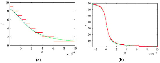
For $\mu =3.8275$ and $c=0.01$, we obtained $E_r=0.1181$ for Equation (7) and $E_r=0.1231$ for Equation (8). For $\mu =3.8284$ and $c=0.01$, we obtained $E_r=0.0949$ and $0.0953$ respectively. We note that Equation (7) approximates more accurately the numerical data. However, as the difference is small, the assumption $q=1$ for $0<\epsilon \ll 1$ can be used without significantly increasing the error.

Now, we can calculate the average laminar length, L, and the characteristic relation, $L\propto {\epsilon }^{\beta }$. We note that previous works reported an exponent $\beta =-1/2$ for type-I intermittency with $\widehat{x}<x_0$ and $\alpha <0$, where $x_0$ is a fixed point [3,42].

Figure 4 shows the characteristic relation for the map (3) and $c=0.01$. The red points are the numerical data, and the blue line is the linear fit, which obtains $\beta =-0.52$. It is very close to the theoretical value given in [3,42].

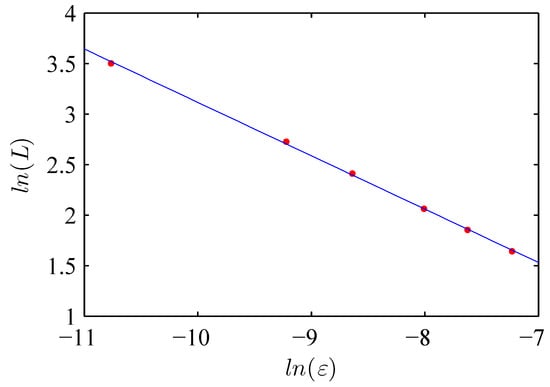
Figure 4. Characteristic relation. Blue line: linear approximation. Red points: numerical data.

Furthermore, in a previous paper, a theoretical method to determine the exponent $\alpha$ was introduced [32]. It uses that the RPD function developed around the extreme points of the map. Supported by this concept, an equation that expresses the exponent $\alpha$ as a function of the number of null derivatives at the map extreme point was found. If we apply this method and evaluate the non-zero lower-order derivative of the map at the pre-reinjection points, we find $\alpha =-0.5$, which is very close to the numerical $\alpha$ (see Table 1).

From the previous results, we highlight that the third iterate of the logistic map generates non-uniform RPD functions, which are described accurately for the M function methodology.

3.2. Fixed Point $x_{02}$

Here, we evaluate the intermittency reinjection around the fixed point $x_{02}$. We moved the map $L_{\mu }^3\left(x\right)$ so that the fixed point $x_{02}$ coincides with the origin of the coordinate system:

$$\begin{array}{cc}F\left(x\right)=\hfill & -x_{02}+{\mu }^3(1-(x+x_{02}))(x+x_{02})(1+\mu (-1+(x+x_{02}))(x+x_{02}))\hfill \\ \\ \hfill & \times (1+{\mu }^2(-1+(x+x_{02}))(x+x_{02})(1+\mu (-1+(x+x_{02}))(x+x_{02}))).\hfill \end{array}$$

(10)

Different reinjection processes can occur. They depend on the laminar interval amplitude, c$(I_l=[-c,c])$, and its relation with $c_l$ and $c_d$. The parameter $c_l$ determines the existence or not of reinjection from neighboring points to $-c$, and it is the limit of the laminar interval length where there are pre-reinjection points close to $-c$. For $c>c_l$, there is no reinjection from neighboring points to points to $-c$, where $c_l$ is obtained from $F(-c_l)-c_l=0$. As an example, for $\mu =3.8275$, $c_l$ results in $c_l\cong 0.057733$. The reinjection process also depends on the relation between c and $c_d$, where ${\left.\frac{dF\left(x\right)}{dx}\right|}_{x=c_d}=0$ and $F\left(c_d\right)\in I_l$. For $\mu =3.8275$, we obtained $c_d\cong -0.014355277$.

To analyze the influence of the relation between c and $c_l$ on the reinjection process, two cases are shown in Figure 5 and Figure 6 for $\mu =3.8275$ and $c=0.04$ and $\mu =3.8275$ and $c=0.06$, respectively. The blue line is the map; the red points are the pre-reinjection points; the green straight lines show the limits of the laminar interval. In Figure 5, there are neighboring pre-reinjection points to the laminar interval. However, these points do not exist in Figure 6.

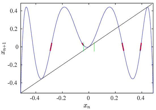
Figure 5. Map and pre-reinjection points for $\mu =3.8275$ and $c=0.04$. Blue line: map. Red points: pre-reinjection points. Green lines: limits of the laminar interval. Black line: bisector.

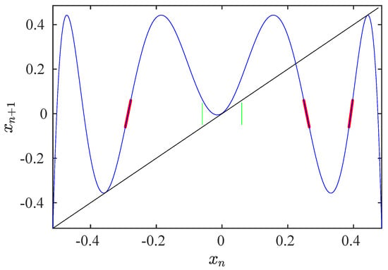
Figure 6. Map and pre-reinjection points for $\mu =3.8275$ and $c=0.06$. Blue line: map. Red points: pre-reinjection points. Green lines: limits of the laminar interval. Black line: bisector.

In addition, for $c<|c_d|$, the RPD function verifies [32]:

$$\varphi \left(x\right)\to \infty ,x\to F\left(c_d\right).$$

(11)

Remember that $c_d$ verifies ${\left.\frac{dF\left(x\right)}{dx}\right|}_{x=c_d}=0$ and $F\left(c_d\right)\in I_l$.

Therefore, we can split the domain of c into three sub-intervals: (a) $|c_d|<c_l<c$, (b) $|c_d|\le c\le c_l$, and (c) $c<|c_d|<c_l$.

We studied the reinjection mechanisms for the three sub-intervals. We start with the simplest case, $|c_d|<c_l<c$.

3.2.1. Sub-Interval $|c_d|<c_l<c$

For this interval, the pre-reinjection points are displayed in Figure 6. Note there is no reinjection from points close to the laminar interval.

Figure 7 shows the RPD obtained by the M function methodology and numerically for $\mu =3.8275$ and $c=0.06$. The blue line is the theoretical RPD, and the red points are the numerical data. We can observe that the RPD is uniform. The exponent $\alpha$ evaluated using the M function methodology is $-0.00976$; therefore, $\alpha \cong 0$, following uniform reinjection.

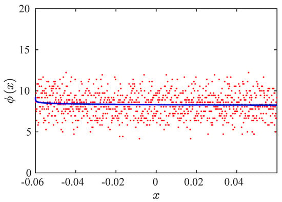
Figure 7. RPD functions for $\mu =3.8275$ and $c=0.06$. Blue line: the RPD calculated by the M function methodology. Red points: numerical results.

From Figure 6, we observe that the map derivatives at the pre-reinjection points are finite and non-zero. Then, following the theoretical development introduced in Ref. [32], we obtained $\alpha =0$. Thus, we found using the M function methodology and theoretically that the RPD should be uniform, which was verified by the numerical results.

3.2.2. Sub-Interval $|c_d|\le c\le c_l$

We highlight in this interval that the map derivative at the pre-reinjection points in the neighborhood of the laminar interval changes rapidly. Therefore, the RPD function is not uniform. To observe it, we can use the Perron–Frobenius technique, which evaluate the RPD function from the derivative at pre-reinjection points [3,46]:

$$\varphi \left(x\right)=\frac{\rho \left(F^{-1}\left(x\right)\right)}{\left|\frac{d{F}^{-1}\left(x\right)}{dx}\right|},$$

(12)

where $\rho \left(F^{-1}\left(x\right)\right)$ is the trajectories’ density at pre-reinjection points.

Therefore, for $c\in \left[\right|c_d|,c_l]$, the RPD has two components. One component is generated by pre-reinjection points distant from the laminar interval. The trajectories passing through these points are reinjected inside the complete laminar interval, $I_l=[-c,c]$. The second component is generated by neighboring pre-reinjection points to the lower limit of the laminar interval, ($x_{n-1}$ close to $-c$). These points verify that $F\left(x_{n-1}\right)\in (F(-c),c]$ (see Figure 5).

To study the reinjection processes, we considered the following test: $\mu =3.8275$ and $|c_d|=0.014355277<c=0.04<c_l=0.057733$. Figure 8 shows the RPD function. The blue line is the theoretical RPD, and the red points are the numerical data.

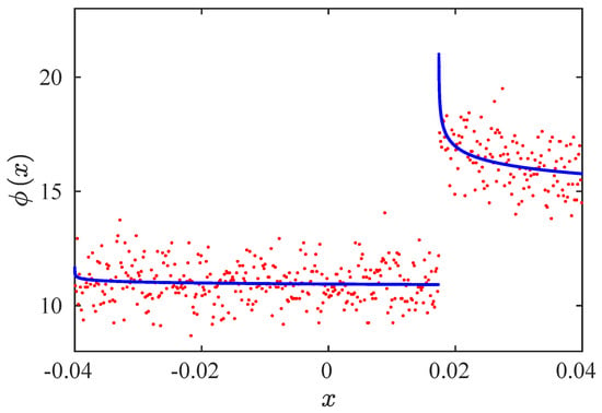
Figure 8. RPD functions for $\mu =3.8275$ and $c=0.04$. Blue line: the RPD calculated by the M function methodology. Red points: numerical results. ${\alpha }_a=-0.00598$, ${\alpha }_b=-0.1011469$.

From this figure, we observe two different behaviors of the RPD function:

(a) For $x_n\in [-c,F(-c)]$, where $F(-c)=0.0173829$. This sub-interval receives the trajectories from $\left|x_{n-1}\right|>c_l$, and the RPD function is similar to those described in the previous subsection;

(b) For $x_n\in (F(-c),c]$. Two mechanisms generate the RPD function. One of them is given by trajectories coming from $\left|x_{n-1}\right|>c_l$, and the second one is produced by trajectories from points $x_{n-1}\in [-c_l,-c)$.

Points from $\left|x_{n-1}\right|>c_l$ are reinjected inside the complete laminar interval $[-c,c]$. However, points from $x_{n-1}\in [-c_l,-c)$ are reinjected in $\left(F\right(-c),c]$.

Figure 9 shows the $M\left(x\right)$ function for the same test as Figure 8. Note that the $M\left(x\right)$ function possesses a non-differentiable point at $F(-c)$, where the RPD is discontinuous.

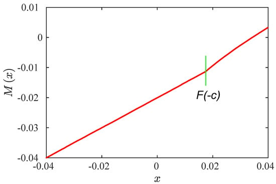
Figure 9. M function for $\mu =3.8275$ and $c=0.04$. The green line corresponds to $x=F(-c)$.

With ${\varphi }_1\left(x\right)$, we restrict the analysis to the interval $\left(F\right(-c),c]$, and ${\varphi }_2\left(x\right)$ is the RPD function inside the interval $[-c,F(-c\left)\right]$. Therefore, the RPD can be written as follows.

$$\varphi \left(x\right)=\left\{\begin{array}{cc}{\varphi }_1\left(x\right)={\varphi }_a\left(x\right)+{\varphi }_b\left(x\right),\hfill & x>F(-c)\hfill \\ {\varphi }_2\left(x\right)={\varphi }_a\left(x\right),\hfill & x\le F(-c),\hfill \end{array}\right.$$

(13)

where:

$$\begin{array}{c}{\varphi }_a\left(x\right)=b{\left(x+c\right)}^{{\alpha }_a}\hfill \\ {\varphi }_b\left(x\right)=bk{\left(x-F(-c)\right)}^{{\alpha }_b}.\hfill \end{array}$$

(14)

The RPD, $\varphi \left(x\right)$, is obtained by adding two reinjection processes described by ${\varphi }_a\left(x\right)$ and ${\varphi }_b\left(x\right)$.

To find the parameters $m_a$ and $m_b$, we studied each reinjection process individually. We ordered the numerical data and applied the M function methodology as explained previously. Therefore, the exponents ${\alpha }_a$ and ${\alpha }_b$ are obtained from:

$${\alpha }_{a,b}=\frac{2m_{a,b}-1}{1-m_{a,b}},$$

(15)

$m_b$ being the slope of the following function:

$$M_b\left(x\right)=m_b\left(x-F(-c)\right)+F(-c),$$

(16)

which is defined in $\left(F\right(-c),c]$, and it considers only reinjected points coming from $[-c_l,c)$; $m_a$ is the slope of:

$$M_a\left(x\right)=m_a\left(x+c\right)-c,$$

(17)

which is evaluated employing only reinjected points’ arrival from $\left|x_{n-1}\right|>c_l$, and it is determined in the entire laminar interval, $I_l=[-c,c]$. Consequently, we can calculate the functions ${\varphi }_a\left(x\right)$ and ${\varphi }_b\left(x\right)$ using Equation (14), where the factor b is the normalization parameter, resulting in:

$$b={\left(\frac{{\left(2c\right)}^{1+{\alpha }_a}}{1+{\alpha }_a}+k\frac{{(c-F(-c))}^{1+{\alpha }_b}}{1+{\alpha }_b}\right)}^{-1}.$$

(18)

To obtain the complete $M\left(x\right)$ function, we again used the M function methodology explained in Appendix B. The complete $M\left(x\right)$ function is provided by Equations (19) and (20). We note that this function possesses a non-differentiable point at $x=F(-c)$.

For $x>F(-c)$:

$$\begin{array}{cc}M\left(x\right)=\hfill & {\displaystyle \frac{{\int }_{-c}^x\tau {\varphi }_a\left(\tau \right)d\tau +{\int }_{F(-c)}^x\tau {\varphi }_b\left(\tau \right)d\tau }{{\int }_{-c}^x{\varphi }_a\left(\tau \right)d\tau +{\int }_{F(-c)}^x{\varphi }_b\left(\tau \right)d\tau }}\hfill \\ \\ =\hfill & \frac{{(c+x)}^{1+{\alpha }_a}(-c+x(1+{\alpha }_a))(1+{\alpha }_b)(2+{\alpha }_b)+k{(x-F(-c))}^{1+{\alpha }_b}(F(-c)+x(1+{\alpha }_b))(1+{\alpha }_a)(2+{\alpha }_a)}{(2+{\alpha }_a)(2+{\alpha }_b)({(c+x)}^{1+{\alpha }_a}(1+{\alpha }_b)+k{(x-F(-c))}^{1+{\alpha }_b}(1+{\alpha }_a))}.\hfill \end{array}$$

(19)

For $x\le F(-c)$:

$$\begin{array}{c}M\left(x\right)={\displaystyle \frac{{\int }_{-c}^x\tau {\varphi }_a\left(\tau \right)d\tau }{{\int }_{-c}^x{\varphi }_a\left(\tau \right)d\tau }}=\frac{x(1+{\alpha }_a)-c}{2+{\alpha }_a}.\hfill \end{array}$$

(20)

The factor k is included to take into account the different number of reinjections inside the intervals $[-c,F(-c\left)\right]$ and $\left(F\right(-c),c]$. This factor is calculated from the definition of $M\left(x\right)$. From Equation (19), we note that the $M\left(x\right)$ function is independent of the parameter b, then we can evaluate k from it:

$$k=\frac{\frac{(-c+x(1+{\alpha }_a)){(x+c)}^{1+{\alpha }_a}}{(1+{\alpha }_a)(2+{\alpha }_a)}-\frac{M\left(x\right){(x+c)}^{1+{\alpha }_a}}{(1+{\alpha }_a)}}{\frac{M\left(x\right){(x-F(-c))}^{1+{\alpha }_b}}{(1+{\alpha }_b)}-\frac{(F(-c)+x(1+{\alpha }_b)){(x-F(-c))}^{1+{\alpha }_b}}{(1+{\alpha }_b)(2+{\alpha }_b)}}.$$

(21)

We calculated Equation (21) for all reinjected points in $\left(F\right(-c),c]$, and we obtained k by the arithmetic average of them.

The laminar length can be obtained from Equation (6). Due to the map symmetry around a vertical line passing through $c_d$, there are two intervals. The first one is given for $x\in [c_d,c]$ and the second one for $x\in [-c,c_d)$.

Therefore, we obtained for $[c_d,c]$:

$$l(x,c)=1+\frac{2arctan\left[\frac{q-1+2ac}{\sqrt{4a\epsilon -{(q-1)}^2}}\right]}{\sqrt{4a\epsilon -{(q-1)}^2}}-\frac{2arctan\left[\frac{q-1+2ax}{\sqrt{4a\epsilon -{(q-1)}^2}}\right]}{\sqrt{4a\epsilon -{(q-1)}^2}}$$

(22)

and for $[-c,c_d)$

$$l(x,c)=1+\frac{2arctan\left[\frac{q-1+2ac}{\sqrt{4a\epsilon -{(q-1)}^2}}\right]}{\sqrt{4a\epsilon -{(q-1)}^2}}-\frac{2arctan\left[\frac{q-1+2a(c_d+\left|x-c_d\right|)}{\sqrt{4a\epsilon -{(q-1)}^2}}\right]}{\sqrt{4a\epsilon -{(q-1)}^2}}.$$

(23)

Figure 10 shows the numerical and theoretical laminar length. The last one is calculated by Equations (22) and (23). Note the symmetry around $x=c_d$, where $c_d=-0.014355277061990445$ for $\mu =3.8275$ and $c_d=-0.014355277061990473$ for $\mu =3.8284$.

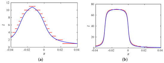
Figure 10. Theoretical and numerical laminar length for $c=0.04$. (a) $\mu =3.8275$. (b) $\mu =3.8284$. Blue points: theoretical evaluation. Red points: numerical data.

The probability density of the laminar lengths, $\psi (l,c)$, is calculated as [3]:

$$\psi (l,c)=\varphi \left(x(l,c)\right)\left|\frac{dx(l,c)}{dl}\right|,$$

(24)

where $\varphi \left(x\right(l,c\left)\right)$ is given by Equations (13) and (14), and $\left|\frac{dx(l,c)}{dl}\right|$ for Equation (6). Figure 11 shows $\psi \left(x\right(l,c\left)\right)$ for two tests with $\mu =3.8275$, and $\mu =3.828$. Blue points are the theoretical evaluation (Equation (24)), and the red points are the numerical data. Note the accuracy between the numerical and theoretical results. Furthermore, these results verify previous works for type-I intermittency [3,42].

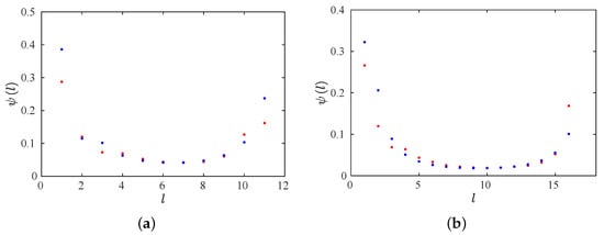
Figure 11. The probability density of the laminar lengths for $c=0.004$. (a) $\mu =3.8275$. (b) $\mu =3.8280$. Blue points: theoretical evaluation. Red points: numerical data.

The characteristic relation, $L=L\left(\epsilon \right)$, is shown in Figure 12. The red points are the numerical results, and the blue line is the linear fit of the numerical data. The slope of the straight blue line is $-0.45$.

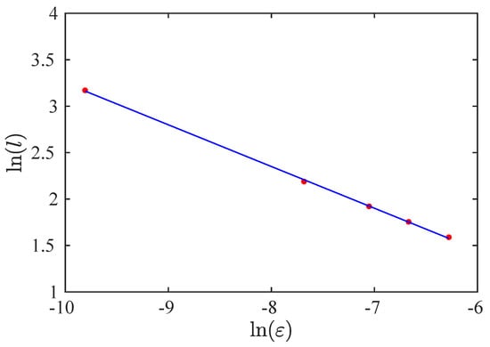
Figure 12. Characteristic relation. Red points: numerical data. Blue line: linear interpolation.

3.2.3. Sub-Interval $c<\left|c_d\right|<c_l$

In this case, the reinjection process has two contributions as described in Section 3.2.2. However, there are some differences.

The first difference happens for a trajectory passing through $c_d$. It is reinjected in $F\left(c_d\right)$, where the RPD tends to infinity (see Equation (12)). Then, the RPD is a discontinuous function at $x=c_d$, and it can be written as:

$$\varphi \left(x\right)=\left\{\begin{array}{cc}{\varphi }_1\left(x\right)={\varphi }_a\left(x\right)+{\varphi }_b\left(x\right),\hfill & x>F\left(c_d\right)\hfill \\ {\varphi }_2\left(x\right)={\varphi }_a\left(x\right),\hfill & x\le F\left(c_d\right),\hfill \end{array}\right.$$

(25)

where:

$$\begin{array}{c}{\varphi }_a\left(x\right)=b{\left(x+c\right)}^{{\alpha }_a}\hfill \\ {\varphi }_b\left(x\right)=bk{\left(x-F\left(c_d\right)\right)}^{{\alpha }_b}.\hfill \end{array}$$

(26)

Note that ${\varphi }_b\left(x\right)$ is determined by $x>F\left(c_d\right)$. This happens because ${\left.\frac{dF\left(x\right)}{dx}\right|}_{x=c_d}=0$, but ${\left.\frac{dF\left(x\right)}{dx}\right|}_{x=-c}>0$ and bounded. Therefore, by Equation (12), the derivative ${\left.\frac{dF\left(x\right)}{dx}\right|}_{x=c_d}$ has a greater influence on the RPD function [46]. Furthermore, $F\left(c_d\right)$ is less than $F(-c)$, but very close to it. As an example, for $\mu =3.8284$, we obtained $F\left(c_d\right)=-0.0071572<F(-c)=-0.00649038$.

The second difference occurs when we analyze the laminar length. As $c_d$ is outside the laminar interval, we did not observe the symmetry around the $c_d$ as in the previous subsection. Then, the theoretical laminar length verifies $\frac{dl\left(x\right)}{dx}<0$ inside the complete laminar interval.

To analyze these differences, we studied theoretical and numerically a test verifying $c<\left|c_d\right|$. We used $\mu =3.8284$ and $c=0.01$, for these values $c_d=-0.014355277$. Figure 13 shows the map and the pre-reinjected points. There is reinjection from points close to the lower boundary of the laminar interval, one of these pre-reinjection points being $x=c_d$.

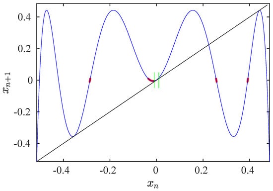
Figure 13. Map and the pre-reinjection points for $\mu =3.8284$ and $c=0.01$. The pre-reinjection points are in red and the map in blue. The green lines show the limits of the laminar interval, and the black line is the bisector.

We used the M function methodology to evaluate the exponents ${\alpha }_a=-0.007144$ and ${\alpha }_b=-0.621795$. Figure 14 shows the theoretical and numerical RPD functions for $N=\mathrm{100,000}$ and $N_s=500$. Note that ${\alpha }_a\approx 0$, as was described previously [3,32].

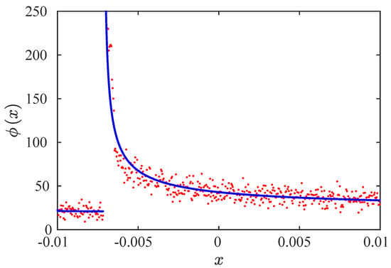
Figure 14. RPD functions for $\mu =3.8284$ and $c=0.01$. Red points: numerical data. Blue line: the RPD calculated by the M function methodology.

The laminar length is shown in Figure 15. We did not observe two intervals in the laminar length distribution because $c_d$ is outside the laminar interval. In all figures, we can note a good accuracy between the numerical data and the theoretical approximation.

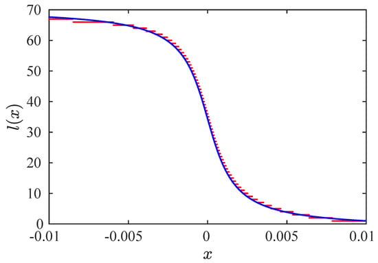
Figure 15. Laminar length for $\mu =3.8284$ and $c=0.01$. Red points: numerical data. Blue line: theoretical result.

4. Conclusions

In this paper, we studied the intermittency reinjection processes for the logistic map. This map exhibits intermittency for $\mu$ just below the Period-3 window. For the third iterate map with $\mu <{\mu }_c=1+\sqrt{8}$, type-I intermittency occurs around three fixed points $x_{01}\cong 0.15992881844625645$, $x_{02}\cong 0.5143552770619905$, and $x_{03}\cong 0.9563178419736238$. By the map symmetry, the reinjection process has different characteristics for $x_{01}$ and $x_{02}$. To describe the reinjection mechanisms, we evaluated by means of the M function methodology the following statistical variables: the reinjection probability density function, $\varphi \left(x\right)$, the laminar length, $l(x,c)$, the probability density of the laminar lengths, $\psi \left(l\right)$, and the characteristic relation, $L\left(\epsilon \right)$.

For $x_{01}$, we verified that the RPD function is given by Equation (4) with $\alpha <0$ because the derivative of the map at a pre-reinjection point is zero, as shown in Figure 1. Therefore, the RPD is far away from the uniform reinjection widely used in classical intermittency. To calculate the laminar length, we approximated the map as a quadratic polynomial around the vanished fixed point (see Equation (5)). As previous studies have established, the linear coefficient was very close to one for small $\epsilon$. Furthermore, for all tests, we found that the lower boundary of reinjection was less than zero, $\widehat{x}<0$ (see Table 1). Finally, we obtained the characteristic relation verifying $L\propto {\epsilon }^{\beta }$ with $\beta \simeq -0.5$, even though the RPD function was not uniform.

On the other hand, the reinjection process for $x_{02}$ depends on the length of the laminar interval and its relationship with both $c_l$ and $c_d$, where $c_l=F(-c_l)$, and $c_d$ verifies ${\left.\frac{dF\left(x\right)}{dx}\right|}_{x=c_d}=0$ with $F\left(c_d\right)\in I_l$. We found that there were three sub-intervals: (a) $c_l<c$, (b) $\left|c_d\right|<c\le c_l$, and (c) $c<\left|c_d\right|<c_l$.

In Sub-interval (a), there is no reinjection from points close to the laminar interval, and the derivative is non-zero and finite at the pre-reinjection points. Then, the RPD function is uniform (constant RPD).

In Sub-interval (b), the RPD function has two components. One of them is generated at pre-reinjection points distant from the laminar interval. These points are reinjected inside the entire laminar interval, $I_l$. The second one is produced by neighboring pre-reinjection points to the lower limit of the laminar interval, $-c$. These points are reinjected in the sub-interval $\left(F\right(-c),c]$. Therefore, the RPD function has two different behaviors, one inside the sub-interval $[c,F(-c\left)\right]$, where the RPD is constant, and the another inside the sub-interval $\left(F\right(-c),c]$, where the RPD is not constant. Another distinctive behavior occurs for the laminar length, $l(x,c)$, which shows symmetry around $c_d$ (see Figure 10). We found that the characteristic relation is $L\propto {\epsilon }^{-0.45}$.

In Sub-interval (c), the RPD function is discontinuous at $F\left(c_d\right)$, and it shows two different behaviors. The RPD is constant in the sub-interval $[-c,F\left(c_d\right)]$, and $\varphi \left(x\right)\propto x^{\alpha }$ with $\alpha <0$ in the sub-interval $(F\left(c_d\right),c]$. In the latter case, the RPD function verifies $\varphi \left(x\right)\to \infty$ when $x^{+}\to F\left(c_d\right)$ (see Figure 14).

We found that the reinjection process depends on the fixed point. The RPD function and other statistical variables can be calculated accurately by the M function methodology. The reinjection mechanism and the RPD function show a more complex behavior than the uniform reinjection. Therefore, for the third iterate of the logistic map, the uniform reinjection assumption can introduce errors in evaluating type-I intermittency.

Finally, we note that the study carried out here can be used to describe the intermittency reinjection process in other maps with several fixed points. Additionally, future works can use this methodology to evaluate the time spent by trajectories around different fixed points.

References

- Schuster, H.; Just, W. Deterministic Chaos; Wiley VCH: Mörlenbach, Germany, 2005. [Google Scholar]
- Nayfeh, A.; Balachandran, B. Applied Nonlinear Dynamics; Wiley: New York, NY, USA, 1995. [Google Scholar]
- Elaskar, S.; del Rio, E. New Advances on Chaotic Intermittency and Its Applications; Springer: Cham, Switzerland, 2017. [Google Scholar]
- Dubois, M.; Rubio, M.; Berge, P. Experimental evidence of intermittencies associated with a subharmonic bifurcation. Phys. Rev. Lett. 1983, 16, 1446–1449. [Google Scholar] [CrossRef]
- Malasoma, J.; Werny, P.; Boiron, M. Multichannel type I intermittency in two models of Rayleigh-Benard convection. Phys. Rev. Lett. 2004, 51, 487–500. [Google Scholar] [CrossRef]
- Stavrinides, S.; Miliou, A.; Laopoulos, T.; Anagnostopoulos, A. The intermittency route to chaos of an electronic digital oscillator. Int. J. Bifurc. Chaos 2008, 18, 1561–1566. [Google Scholar] [CrossRef]
- Zambrano, S.; Perez Mariño, I.; Sanjuan, M. Controlling crisis-induced intermittency using its relation with a boundary crisis. New J. Phys. 2009, 11, 023025. [Google Scholar] [CrossRef]
- Pizza, G.; Frouzakis, C.; Mantzaras, J. Chaotic dynamics in premixed Hydrogen/air channel flow combustion. Combust. Theor. Model. 2012, 16, 275–299. [Google Scholar] [CrossRef]
- Nishiura, Y.; Ueyama, D.; Yanagita, T. Chaotic pulses for discrete reaction diffusion systems. SIAM J. App. Dyn. Syst. 2005, 4, 723–754. [Google Scholar] [CrossRef]
- De Anna, P.; Le Borgne, T.; Dentz, M.; Tartakovsky, A.; Bolster, D.; Davy, P. Flow intermittency, dispersion and correlated continuous time random walks in porous media. Phys. Rev. Lett. 2013, 110, 184502. [Google Scholar] [CrossRef]
- Stan, C.; Cristescu, C.; Dimitriu, D. Analysis of the intermittency behavior in a low-temperature discharge plasma by recurrence plot quantification. Phys. Plasmas 2010, 17, 042115. [Google Scholar] [CrossRef]
- Chian, A. Complex System Approach to Economic Dynamics. Lecture Notes in Economics and Mathematical Systems; Springer: Berlin, Germany, 2007. [Google Scholar]
- Zebrowski, J.; Baranowski, R. Type I intermittency in nonstationary systems: Models and human heart-rate variability. Phys. A 2004, 336, 74–86. [Google Scholar] [CrossRef]
- Paradisi, P.; Allegrini, P.; Gemignani, A.; Laurino, M.; Menicucci, D.; Piarulli, A. Scaling and intermittency of brains events as a manifestation of consciousness. AIP Conf. Proc. 2012, 1510, 151–161. [Google Scholar]
- Batchelor, G.; Townsend, C. The nature of turbulent motion at large wave-number. Proc. R. Soc. London Ser. A 1949, 199, 238–255. [Google Scholar]
- Manneville, P.; Pomeau, Y. Intermittency and the Lorenz model. Phys. Lett. 1979, 75A, 1–2. [Google Scholar] [CrossRef]
- Bauer, M.; Habip, S.; He, D.; Martiessen, W. New type of intermittency in discontinuous maps. Phys. Rev. Lett. 1992, 68, 1625–1628. [Google Scholar] [CrossRef] [PubMed]
- He, D.; Bauer, M.; Habip, S.; Kruger, U.; Martiessen, W.; Christiansen, B.; Wang, B. Type V intermittency. Phys. Lett. A 1992, 171, 61–65. [Google Scholar] [CrossRef]
- Fan, J.; Ji, F.; Guan, S.; Wang, B.; He, D. The distribution of laminar lenghts in type V intermittency. Phys. Lett. A 1993, 182, 232–237. [Google Scholar] [CrossRef]
- Price, T.; Mullin, P. An experimental observation of a new type of intermittency. Phys. D 1991, 48, 29–52. [Google Scholar] [CrossRef]
- Platt, N.; Spiegel, E.; Tresser, C. On-off intermittency: A mechanism for bursting. Phys. Rev. Lett. 1993, 70, 279–282. [Google Scholar] [CrossRef]
- Heagy, J.; Platt, N.; Hammel, S. Characterization of on–off intermittency. Phys. Rev. E 1994, 49, 1140–1150. [Google Scholar] [CrossRef]
- Pikovsky, A.; Osipov, G.; Rosenblum, M.; Zaks, M.; Kurths, J. Attractor–repeller collision and eyelet intermittency at the transition to phase synchronization. Phys. Rev. Lett. 1997, 79, 47–50. [Google Scholar] [CrossRef]
- Pikovsky, A.; Rosenblum, M.; Kurths, J. Synchronization. A Universal Concept in Nonlinear Sciences; Cambridge University Press: New York, NY, USA, 2001. [Google Scholar]
- Kurovskaya, M. Distribution of laminar phases at eyelet-type intermittency. Tech. Phys. Lett. 2008, 34, 1063–1065. [Google Scholar] [CrossRef]
- Hramov, A.; Koronovskii, A.; Kurovskaya, M.; Boccaletti, S. Ring intermittency in coupled chaotic oscillators at the boundary of phase synchronization. Phys. Rev. Lett. 2006, 97, 114101. [Google Scholar] [CrossRef] [PubMed]
- Hirsch, J.; Huberman, B.; Scalapino, D. Theory of intermittency. Phys. Rev. A 1982, 25, 519–532. [Google Scholar] [CrossRef]
- Elaskar, S.; del Rio, E.; Donoso, J. Reinjection probability density in type III intermittency. Phys. A 2011, 390, 2759–2768. [Google Scholar] [CrossRef]
- Krause, G.; Elaskar, S.; del Rio, E. Noise effect on statistical properties of type I intermittency. Phys. A 2014, 402, 318–329. [Google Scholar] [CrossRef]
- Elaskar, S.; del Río, E.; Krause, G.; Costa, A. Effect of the lower boundary of reinjection and noise in type II intermittency. Nonlinear Dynam. 2015, 79, 1411–1424. [Google Scholar] [CrossRef]
- Elaskar, S.; del Rio, E. Discontinuous reinjection probability density function in type V intermittency. J. Comp. Nonlinear Dynam. 2018, 13, 121001. [Google Scholar] [CrossRef]
- Del Río, E.; Elaskar, S. On the intermittency theory. Int. J. Bifurc. Chaos 2016, 26, 1650228. [Google Scholar] [CrossRef]
- Bragard, J.; Vélez, J.; Riquelme, J.; Barrientos, R.; Laroze, D. Study of type-III intermittency in the Landau-Lifshitz-Gilbert equation. Phys. Scr. 2021, 96, 124045. [Google Scholar] [CrossRef]
- Ge, P.; Cao, H. Intermittent evolution routes to the periodic or the chaotic orbits in Rulkov map. Chaos 2021, 31, 093119. [Google Scholar] [CrossRef]
- Belyaev, I.; Biryukov, D.; Gerasimov, D.; Yurin, E. On-off intermittency and hard turbulence in the flow of fluid in the magnetic field. Chaos 2019, 29, 083119. [Google Scholar] [CrossRef]
- Bordbar, P.; Ahadpour, S. Type-I intermittency from Markov binary block visibility graph perspective. J. Appl. Stat. 2021, 48, 1303–1318. [Google Scholar] [CrossRef]
- Kong, L.; Fan, H.; Grebogi, C.; Lai, Y. Emergence of transient chaos and intermittency in machine learning. J. Phys. Complex. 2021, 035014, 16. [Google Scholar] [CrossRef]
- Strogatz, S. Nonlinear Dynamics and Chaos; Perseus Book Publishing: Cambridge, UK, 1994. [Google Scholar]
- Sternberg, S. Dynamical Systems; Dover Publications: New York, NY, USA, 2010. [Google Scholar]
- May, R. Simple mathematical model with very complicated dynamics. Nature 1976, 261, 459. [Google Scholar] [CrossRef] [PubMed]
- Del Rio, E.; Elaskar, S.; Makarov, S. Theory of intermittency applied to classical pathological cases. Chaos 2013, 23, 033112. [Google Scholar] [CrossRef] [PubMed]
- Del Rio, E.; Elaskar, S.; Donoso, J. Laminar length and characteristic relation in type I intermittency. Commun. Nonlinear Sci. Numer. Simulat. 2014, 19, 967–976. [Google Scholar] [CrossRef]
- Shukla, A.; Patel, R. Controllability results for fractional semilinear delay control systems. J. Appl. Math. Comput. 2021, 65, 861–875. [Google Scholar] [CrossRef]
- Shukla, A.; Sukavanam, N.; Pandey, D. Approximate controllability of semilinear fractional stochastic control system. Asian-Eur. J. Math. 2018, 11, 1850088. [Google Scholar] [CrossRef]
- Blokh, A.; Fokkink, R.; Mayer, J.; Oversteegen, L.; Tymchatyn, E. Fixed Point Theorems for Plane Continua with Applications. Mem. Am. Math. Soc. 2013, 224, 1053. [Google Scholar] [CrossRef]
- Elaskar, S.; del Rio, E.; Lorenzon, D. Calculation of the Statistical Properties in Intermittency Using the Natural Invariant Density. Symmetry 2021, 13, 935. [Google Scholar] [CrossRef]
Publisher’s Note: MDPI stays neutral with regard to jurisdictional claims in published maps and institutional affiliations. |
© 2022 by the authors. Licensee MDPI, Basel, Switzerland. This article is an open access article distributed under the terms and conditions of the Creative Commons Attribution (CC BY) license (https://creativecommons.org/licenses/by/4.0/).