Interpolating Scaling Functions Tau Method for Solving Space–Time Fractional Partial Differential Equations

Abstract

This paper is devoted to an innovative and efficient technique for solving space–time fractional differential equations (STFPDEs). To this end, we apply the Tau method such that the bases used are interpolating scaling functions (ISFs). The operational metrics for the derivative operator and fractional integration operator are used to introduce the operational matrix for the Caputo fractional derivative. Due to some characteristics of ISFs, such as interpolation, computation costs can be significantly reduced. We investigate the convergence of the technique, and some numerical implementations show that the method is effective for solving such equations.

1. Introduction

Our objective is to introduce an efficient method to find the numerical solution for the space–time fractional partial differential equation STFPDEs

$$a_1\frac{{\partial }^{\beta }w(x,t)}{\partial t^{\beta }}+a_2\frac{{\partial }^{\alpha }w(x,t)}{\partial x^{\alpha }}=g(x,t),\alpha ,\beta \in [0,1],t\ge 0,x\in [0,1],$$

(1)

subject to the initial condition

$$w(x,0)=w_0\left(x\right),x\in [0,1],$$

and the boundary condition

$$w(0,t)=f_1\left(t\right),t\ge 0,$$

in which $a_1$ and $a_2$ are constants. In addition, the function $g(x,t)$ in (1) is assumed to be sufficiently smooth.

In recent decades, the generalization of differentiation has given rise to finding a new class of differential equations. Nowadays, we can imagine a significant role for fractional calculus and fractional differential and integral operators in various fields of science. Therefore, it is important to study this topic. In the field of solving fractional differential equations (FDE), an exact solution in many cases is not possible. Thus, introducing an efficient and precise numerical scheme is significant. For the one-dimensional fractional differential equations, several papers are dedicated to specifying the necessary and sufficient conditions for the existence and uniqueness of the solution [1,2]. Several papers introduced various approximation techniques for solving this type of equation. Among these, one can mention finite difference methods [3], wavelet method [1], Laplace transform method [4], B-spline method [5], tau method [6], Homotopy analysis method [7], and Adomian’s decomposition method [8], etc.

In [5], the authors represented the fractional derivatives based on B-spline functions as an operational matrix. Then, they solved the fractional ODEs and STFPDEs using this matrix. The operational matrix in this work is introduced directly, and they did not use the operational matrix of integration like the method presented in this paper. In [9], the authors solved the time-fractional diffusion equation

$${}^c{\mathcal{D}}_0^{\beta }w(x,t)={\mathcal{D}}^{2}w(x,t)+f(x,t),$$

where ${}^c{\mathcal{D}}_0^{\beta }$ denotes the Caputo fractional derivative (Cfd). To apply the numerical technique proposed in [9], the desired equation is discretized by the spectral method in space and the finite difference method in time. Saadatmandi et al. [10] used the Sinc–Legendre collocation method to solve the time-fractional convection-diffusion equation. In [11], the authors used the differential transform method for solving linear fractional PDEs. In [12], the time-fractional reaction–diffusion equations are solved by a numerical scheme. Chen et al. [13] applied the wavelet method to solve the convection–diffusion equation of the fractional order. The space fractional diffusion equation is solved by the adomian decomposition method in [14]. In [15], a Tau method is developed to solve the space fractional diffusion equation. As we have said, various methods have been used in the literature to solve PDEs of the fractional order, including He’s variational iteration method [16], homotopy analysis method [17], and finite element methods [18], etc.

Interpolating scaling functions have an extensive background in applied mathematics and in solving different types of differential equations. Alpert introduced these functions and used them to solve the integral equation with a weakly singular kernel [19]. To simulate the squeezing nanofluid flow, these bases are used and numerical solutions with high accuracy are obtained from them [20]. Asadzadeh et al. [1] used these bases to solve the generalized Cauchy problem.

The outline of this article is as follows. In Section 2, the interpolating scaling functions (ISFs) and their properties are introduced. Section 3 is dedicated to applying the Tau method for solving STFPDEs based on ISFs, and the convergence analysis is investigated for the proposed method. Numerical results are given in Section 4 to demonstrate the ability and efficiency of the method.

2. Interpolating Scaling Functions

Given a set of r roots $\{{\tau }_{\eta }:\eta \in \mathcal{R}\}$ of the Legendre polynomial $P_r$ where $\mathcal{R}=\{0,1,\cdots ,r-1\}$, the Lagrange basis for nodes $\{{\tau }_{\eta }:\eta \in \mathcal{R}\}$ is the set of polynomials $\{l_{\eta }:\eta \in \mathcal{R}\}$, which are described by

$$l_{\eta }\left(x\right)=\prod _{i=0,i\ne \eta }^{r-1}\frac{x-{\tau }_i}{{\tau }_{\eta }-{\tau }_i}.$$

Now, we can define the interpolating scaling functions (ISFs) as a family of orthonormal basis via

$${\psi }^{\eta }\left(x\right)=\left\{\begin{array}{cc}\sqrt{\frac{2}{{\omega }_{\eta }}}{l}_{\eta }(2x-1),& x\in [0,1],\hfill \\ 0,& \mathrm{otherwise},\hfill \end{array}\right.$$

in which ${\omega }_{\eta }$ is the Gauss–Legendre quadrature weight and is obtained by

$${\omega }_{\eta }=\frac{2}{r{P^{\prime }}_r\left({\tau }_{\eta }\right)P_{r-1}\left({\tau }_{\eta }\right)}.$$

There is a subspace $A_0^r$ of the space $L^2[0,1]$ that is generated by $\{{\psi }^{\eta }:\eta \in \mathcal{R}\}$,

$$A_0^r:=\mathit{span}\{{\psi }^{\eta }:\eta \in \mathcal{R}\}\subset L^2[0,1].$$

Given $J\in {\mathbb{N}}_0$ (natural numbers with zero), we consider $I_{J,b}:=[z_b,z_{b+1}]$ with $z_b:=b/\left(2^J\right)$ as a finite number of sub-intervals of the interval [0,1], so that $[0,1]={\cup }_{b\in {\mathcal{B}}_J}{I}_{J,b}$ and $b\in {\mathcal{B}}_J:=\{0,\cdots ,2^J-1\}$. Further, we define the translation and dilation operators:

$${\mathcal{T}}_{b}f\left(x\right)=f(x-b),\mathrm{and}{\mathcal{D}}_{a}f\left(x\right)=\sqrt{a}f\left(ax\right),\mathrm{respectively}.$$

It follows from the multi-resolution analysis (MRA) that there exist the nested subspaces

$$A_j^r=span\{{\psi }_{j,b}^{\eta }:={\mathcal{D}}_{2^j}{\mathcal{T}}_b{\psi }^{\eta },b\in {\mathcal{B}}_j,\eta =0,1,\cdots ,r-1\},$$

such that $A_j^r\subset A_{j+1}^r$. Therefore, the subspace $A_j^r$ is generated by a family of orthonormal bases such that they are the dilation and translation version of the primal basis $\{{\psi }^{\eta }:\eta \in \mathcal{R}\}$.

There exists an orthogonal projection operator ${\mathcal{P}}_J^r$ so that any function $g\left(x\right)$ can be mapped from $L^2[0,1]$ into $A_J^r$, i.e.,

$$g\approx {\mathcal{P}}_J^r\left(g\right)=\sum _{b\in {\mathcal{B}}_J}\sum _{\eta \in \mathcal{R}}{⟨g,{\psi }_{J,b}^{\eta }⟩}_{L^2[0,1]}{\psi }_{J,b}^{\eta },g\in L_2[0,1],$$

(2)

where $⟨.,.⟩$ denotes the $L^2$-inner product

$$⟨g_1,g_2⟩={\int }_0^1{g}_1\left(x\right)g_2\left(x\right)dx.$$

However, in this system, we avoid calculating the integrals due to the interpolating property of ISFs, and instead of calculating $g_{J,b}^{\eta }:={⟨g,{\psi }_{J,b}^{\eta }⟩}_{L^2[0,1]}={\int }_{I_{J,b}}g\left(x\right){\psi }_{J,b}^r\left(x\right)dx$, these coefficients are approximated by

$$g_{J,b}^{\eta }\approx 2^{-J/2}\sqrt{\frac{{\omega }_{\eta }}{2}}g\left(2^{-J}({\widehat{\tau }}_{\eta }+b)\right),b\in {\mathcal{B}}_J,\eta \in \mathcal{R},\mathrm{and}{\widehat{\tau }}_{\eta }:=({\tau }_{\eta }+1)/2.$$

(3)

It can be verified that the convergence rate for the projection ${\mathcal{P}}_J^r$ is $O\left(2^{-Jr}\right)$ [19], and we have the following error estimate:

$$\parallel {\mathcal{P}}_J^r\left(g\right)-g\parallel \le 2^{-Jr}\frac{2}{4^{r}r!}\underset{x\in [0,1]}{sup}\left|g^{\left(r\right)}\left(x\right)\right|,$$

(4)

where $g\in {\mathbb{C}}^r\left([0,1]\right)$ is the r-times continuously differentiable function.

All these calculations can also be expressed in matrix form. Given $b_{max}:=maxb\in {\mathcal{B}}_J$, let us consider the vector function ${\mathsf{\Psi }}_J^r:={[{\mathsf{\Psi }}_{J,0}^r,\cdots ,{\mathsf{\Psi }}_{J,b_{max}}^r]}^T$ with ${\mathsf{\Psi }}_{J,b}^r:=[{\psi }_{J,b}^0,\cdots ,{\psi }_{J,b}^{r-1}]$ consisting of the scaling functions with dimension $N:=r{2}^J$. According to these assumptions, Equation (2) can be rewritten as

$${\mathcal{P}}_J^r\left(g\right)=G^T{\mathsf{\Psi }}_J^r,$$

(5)

where G is an $N\times N$ vector whose elements are obtained by (3). These calculations can be easily extended to higher spaces. To approximate a two-dimensional function, we introduce the two-dimensional subspace $A_J^{r,2}:=A_J^r\times A_J^r\subset L^2{[0,1]}^2$ that is generated by

$$\{{\psi }_{J,b}^{\eta }{\psi }_{J,b^{\prime }}^{{\eta }^{\prime }}:b,b^{\prime }\in {\mathcal{B}}_J,\eta ,{\eta }^{\prime }\in \mathcal{R}\}.$$

Therefore, it can be shown that the mapping of any two-dimensional function g into the space $A_J^{r,2}$ can be written as a linear expansion as follows.

$$g\approx {\mathcal{P}}_J^r\left(g\right)=\sum _{b\in {\mathcal{B}}_j}\sum _{{\eta }^{\prime }\in \mathcal{R}}\sum _{b^{\prime }\in {\mathcal{B}}_j}\sum _{\eta \in \mathcal{R}}{G}_{r(b-\alpha 2^J)+(\eta +1),r(b^{\prime }-\alpha 2^J)+({\eta }^{\prime }+1)}{\psi }_{J,b}^{\eta }\left(x\right){\psi }_{J,b^{\prime }}^{{\eta }^{\prime }}\left(y\right)={{\mathsf{\Psi }}_J^r}^T\left(x\right)G{\mathsf{\Psi }}_J^r\left(y\right),$$

(6)

in which G is a square matrix whose components are obtained by

$$G_{r(b-\alpha 2^J)+(\eta +1),r(b^{\prime }-\alpha 2^J)+({\eta }^{\prime }+1)}\approx 2^{-J}\sqrt{\frac{{\omega }_{\eta }}{2}}\sqrt{\frac{{\omega }_{{\eta }^{\prime }}}{2}}g\left(2^{-J}({\widehat{\tau }}_{\eta }+b),2^{-J}({\widehat{\tau }}_{{\eta }^{\prime }}+b^{\prime })\right).$$

(7)

It has been investigated in references [21,22,23] that the error of this approximation is bounded and satisfies the following boundary.

$$\parallel {\mathcal{P}}_J^{r}g-g\parallel \le {\mathcal{C}}_{max}\frac{2^{1-rJ}}{4^{r}r!}\left(2+\frac{2^{1-Jr}}{4^{r}r!}\right),$$

(8)

where ${\mathcal{C}}_{max}$ is a constant and the function $g:=L^2{[0,1]}^2\to \mathbb{R}$ possesses mixed $2r$ order partial derivatives, which are continuous.

2.1. The Operational Matrix of Derivative

In this section, we would like to find an $N\times N$ dimensional matrix $D_{\psi }$, so that

$$\mathcal{D}\left({\mathsf{\Psi }}_J^r\right)\left(x\right)=D_{\psi }{\mathsf{\Psi }}_J^r\left(x\right),$$

(9)

where $\mathcal{D}$ is used to express the derivative operator. Motivated by [21,22], we can find $D_{\psi }$ (operational matrix of the derivative) as a block-tridiagonal matrix of form

$$D_{\psi }=2^J{\left[\begin{array}{cccccc}\underline{H}& R& & & & \\ -R^T& H& R& & & \\ & \ddots & \ddots & \ddots & & \\ & & \ddots & \ddots & \ddots & \\ & & & -R^T& H& R\\ & & & & -R^T& \overline{H}\end{array}\right]}_{N\times N},$$

in which each block is an $r\times r$ matrix with elements

$$\begin{array}{cc}\hfill {\left[\underline{H}\right]}_{k+1,l+1}& =\frac{1}{2}{\psi }^l\left(1\right){\psi }^k\left(1\right)-{\psi }^l\left(0\right){\psi }^k\left(0\right)-q_{k+1,l+1},\hfill \\ \hfill {\left[H\right]}_{k+1,l+1}& =\frac{1}{2}{\psi }^l\left(1\right){\psi }^k\left(1\right)-\frac{1}{2}{\psi }^l\left(0\right){\psi }^k\left(0\right)-q_{k+1,l+1},\hfill \\ \hfill {\left[\overline{H}\right]}_{k+1,l+1}& ={\psi }^l\left(1\right){\psi }^k\left(1\right)-\frac{1}{2}{\psi }^l\left(0\right){\psi }^k\left(0\right)-q_{k+1,l+1},\hfill \\ \hfill {\left[R\right]}_{k+1,l+1}& =\frac{1}{2}{\psi }^l\left(0\right){\psi }^k\left(1\right),\hfill \\ \hfill {\left[q\right]}_{k+1,l+1}& =\sqrt{\frac{{\omega }_l}{2}}\frac{d}{dt}{\psi }^k\left({\widehat{\tau }}_l\right).\hfill \end{array}$$

2.2. Operational Matrix of Fractional Derivative

By taking the fractional integral of the vector function ${\mathsf{\Psi }}_J^r\left(x\right)$ and expanding the results based on these bases (namely, ${\mathsf{\Psi }}_J^r\left(x\right)$), one can find an N-dimensional square matrix such that

$${\mathcal{I}}_0^{\beta }\left({\mathsf{\Psi }}_J^r\left(x\right)\right)\approx I^{\beta }{\mathsf{\Psi }}_J^r\left(x\right),x\in (0,1),$$

(10)

where the matrix $I^{\beta }$ is used to represent the operational matrix of the fractional integral. It follows from [2] that the fractional integral operator ${\mathcal{I}}_a^{\beta }$ is defined as follows.

Definition 1.

Let $\beta \in {\mathbb{R}}^{+}$. We specify the fractional integral operator ${\mathcal{I}}_a^{\beta }$ via

$${\mathcal{I}}_a^{\beta }\left(f\right)\left(x\right):=\frac{1}{\mathsf{\Gamma }\left(\beta \right)}{\int }_a^x{(x-\zeta )}^{\beta -1}f\left(\zeta \right)d\zeta ,x\in [a,b],f\in L_1[a,b].$$

(11)

Throughout the paper, we will use $\mathsf{\Gamma }\left(\beta \right)$ to represent the gamma function. Our objective is to find the elements of matrix $I^{\beta }$. To this end, we provide the following auxiliary Lemma.

Lemma 1

(cf. [1]). Given a set of r nodes ${\left\{{\tau }_m\right\}}_{m\in \mathcal{R}}\in [0,1]$, the Lagrange polynomials $l_m$ for those nodes can be explicitly given by

$$l_m\left(x\right)=\sum _{n=0}^{r-1}{\beta }_{m,n}{x}^{r-n-1},m=0,\cdots ,r-1,$$

(12)

in which ${\beta }_{m,0}=1/\left({\prod }_{n^{\prime }=0,n^{\prime }\ne m}^{r-1}({\tau }_m-{\tau }_{n^{\prime }})\right)$ and

$${\beta }_{m,n}=\frac{{(-1)}^n}{{\prod }_{n^{\prime }=0,n^{\prime }\ne m}^{r-1}({\tau }_m-{\tau }_{n^{\prime }})}\sum _{m_n=m_{n-1}+1}^{r-1}\cdots \sum _{m_1=0}^{r-n-2}\prod _{i^{\prime }=1}^n{\tau }_{m_{i^{\prime }}},\begin{array}{c}n=1,\cdots ,r-1,\hfill \\ m\ne m_1\ne \cdots \ne m_n.\hfill \end{array}$$

Now, putting $i=br+m+1$, $j=b^{\prime }r+m^{\prime }+1$ where $m,m^{\prime }\in \mathcal{R}$ and $b,b^{\prime }\in {\mathcal{B}}_J$, the entries of the matrix $I^{\beta }$ can be computed by [1]

$$\begin{array}{cc}\hfill {\left[I^{\beta }\right]}_{i,j}& =2^{\frac{-J}{2}}\sqrt{\frac{{\omega }_{m^{\prime }}}{2}}{\mathcal{I}}^{\beta }\left({\psi }_{J,b}^r\right)\left(2^{-J}({\widehat{\tau }}_{m^{\prime }}+b^{\prime })\right)\hfill \\ \hfill & =\frac{2^{\frac{-J}{2}}}{\mathsf{\Gamma }\left(\beta \right)}\sqrt{\frac{{\omega }_{m^{\prime }}}{2}}{\int }_0^{2^{-J}(\widehat{{\tau }_{m^{\prime }}}+b^{\prime })}{(2^{-J}({\widehat{\tau }}_{m^{\prime }}+b^{\prime })-t)}^{\beta -1}{\psi }_{J,b}^r\left(t\right)dt.\hfill \end{array}$$

(13)

Notice that due to the formulation of ISFs, these bases are discontinuous. However, they are locally integrable, and their fractional integral are well-defined. In [1], Asadzadeh et al. evaluate this integral and verify that the matrix $I^{\beta }$ is an upper triangular matrix whose elements are obtained by considering three cases. We refer the reader to [1] for more details.

Case (1):

$b^{\prime }<b$. In this case, which includes elements below the main diagonal, we have

$${\left[I^{\beta }\right]}_{i,j}=0,i,j=1,\cdots ,N.$$

(14)

Case (2):

$b^{\prime }=b$. This case consists of those elements that lie on the diagonal. To evaluate the integrals in this case, using the beta function B, we obtain

$${\left[I^{\beta }\right]}_{i,j}=\frac{{\left(2^{-J}\lambda \right)}^{\beta }}{\mathsf{\Gamma }\left(\beta \right)}\sqrt{\frac{{\omega }_{m^{\prime }}}{{\omega }_m}}B(1,\beta )\sum _{n=0}^{r-1}{\beta }_{m,n}{(-1)}^{r-n-l}{}_2{\mathcal{F}}_1(n+1-r,1;\beta +1;2\lambda ),$$

(15)

where ${}_2{\mathcal{F}}_1(n+1-r,1;\beta +1;2\lambda )$ is the hypergeometric function and is determined by

$${}_2{\mathcal{F}}_1(n+1-r,1;\alpha +1;2\lambda )=\sum _{k=0}^{r-n-1}{(-1)}^k\left(\begin{array}{c}r-n-l\\ k\end{array}\right)\frac{{\left(1\right)}_k}{{(\beta +1)}_k}{\left(2\lambda \right)}^k.$$

(16)

Case (3):

$b^{\prime }>b$. The components of this case lie above the main diagonal and are calculated in reference [1] as follows.

$$\begin{array}{cc}\hfill {\left[I^{\beta }\right]}_{i,j}& =\frac{{\left(2^{-J}\lambda \right)}^{\beta }}{\mathsf{\Gamma }\left(\beta \right)}\sqrt{\frac{{\omega }_{m^{\prime }}}{{\omega }_m}}\sum _{n=0}^{r-1}{\beta }_{m,n}\sum _{k=0}^{r-1-n}\left(\begin{array}{c}r-1-n\\ k\end{array}\right){\left(2\lambda \right)}^{r-1-n-k}{(-1)}^k\hfill \\ \hfill & \times \frac{{(1/\lambda )}^{\sigma }}{\sigma }{}_2{\mathcal{F}}_1(\sigma ,1-\beta ;\sigma +1;1/\lambda ),\hfill \end{array}$$

(17)

where $\sigma :=r-l-m$.

Definition 2

([2,24]). We specify the Caputo fractional derivative (Cfd) ${}^c{\mathcal{D}}_a^{\beta }$ via

$$\begin{array}{cc}\hfill {}^c{\mathcal{D}}_a^{\beta }\left(f\right)\left(x\right):& =\frac{1}{\mathsf{\Gamma }(n-\beta )}{\int }_a^x\frac{f^{\left(n\right)}\left(\zeta \right)d\zeta }{{(x-\zeta )}^{\beta -n+1}}=:{\mathcal{I}}_a^{n-\beta }{\mathcal{D}}^n\left(f\right)\left(x\right),\hfill \end{array}$$

(18)

in which $\beta \in {\mathbb{R}}^{+}$ and $\left[\beta \right]+1:=n\in \mathbb{N}$.

Lemma 2

(cf. Corollary 2.3 (a), [2]). It can be proved that the Cfd operator ${}^c{\mathcal{D}}_a^{\beta }$ is bounded via

$${\parallel {}^c{\mathcal{D}}_a^{\beta }\left(f\right)\parallel }_C\le \frac{1}{\mathsf{\Gamma }(n-\beta )(n-\beta +1)}{\parallel f\parallel }_{C^n},$$

(19)

where $\beta \in {\mathbb{R}}^{+}$, $\beta \notin {\mathbb{N}}_0$ and $n=-[-\beta ]$.

Similar to the operational matrix for fractional integration $I^{\beta }$, there exists a square matrix $D^{\beta }$ of dimension N such that it satisfies the following relation.

$${}^c{\mathcal{D}}_a^{\beta }\left(\mathsf{\Psi }\left(x\right)\right)\approx D^{\beta }\mathsf{\Psi }\left(x\right).$$

(20)

It follows from Definition 2 that there is a relation between the fractional integral operator and the Cfd operator as follows:

$${}^c{\mathcal{D}}_a^{\beta }={\mathcal{I}}_a^{n-\beta }{\mathcal{D}}^n.$$

(21)

Motivated by (9), (10) and using Equation (21), we obtain

$${}^c{\mathcal{D}}_a^{\beta }\left(\mathsf{\Psi }\left(x\right)\right)\approx D^n\left(I^{n-\beta }\right)\mathsf{\Psi }\left(x\right),$$

(22)

In the sequel, the operational matrix for Cfd is equal to

$$D^{\beta }=D^n\left(I^{n-\beta }\right).$$

(23)

3. Tau Method

To solve the space-time fractional partial differential Equation (1), assume that the function $w(x,t)$ can be approximated by

$$w(x,t)\approx w_J^r(x,t):={\mathcal{P}}_J^r\left(w\right)(x,t)=\sum _{b\in {\mathcal{B}}_j}\sum _{{\eta }^{\prime }\in \mathcal{R}}\sum _{b^{\prime }\in {\mathcal{B}}_j}\sum _{\eta \in \mathcal{R}}{W}_{r(b-\alpha 2^J)+(\eta +1),r(b^{\prime }-\alpha 2^J)+({\eta }^{\prime }+1)}{\psi }_{J,b}^{\eta }\left(x\right){\psi }_{J,b^{\prime }}^{{\eta }^{\prime }}\left(y\right)$$

(24)

Using the definition of the vector function ${\mathsf{\Psi }}_J^r$, one can rewrite Equation (24) as follows.

$$w_J^r(x,t)={{\mathsf{\Psi }}_J^r}^T\left(x\right)W{\mathsf{\Psi }}_J^r\left(y\right),$$

(25)

where W is the $N\times N$ matrix.

Substituting the approximate solution (25) in (1), we obtain

$$a_1\frac{{\partial }^{\beta }{w}_J^r(x,t)}{\partial t^{\beta }}+a_2\frac{{\partial }^{\alpha }{w}_J^r(x,t)}{\partial x^{\alpha }}=g_J^r(x,t),$$

(26)

where

$$g(x,t)\approx g_J^r(x,t)={\mathsf{\Psi }}_J^r\left(x\right)G{\mathsf{\Psi }}_J^r\left(t\right).$$

Employing the operational matrix $D^{\beta }$, one can obtain the residual function via

$$r(x,t):={\mathsf{\Psi }}_J^r\left(x\right)\left(a_{1}W{D}^{\beta }+a_2{D^{\alpha }}^{T}W-G\right){\mathsf{\Psi }}_J^r\left(t\right).$$

(27)

We aim to force $r(x,t)$ to be approximately zero. To do this, we adopt the Tau method to obtain the linear system of algebraic equations, i.e.,

$$\mathrm{Y}\left(W\right):=a_{1}W{D}^{\beta }+a_2{D^{\alpha }}^{T}W-G=0.$$

(28)

Equation (28) consists of $2N+1$ dependent equations. Therefore, the boundary and initial conditions are used to find $2N+1$ independent linear equations.

$$\begin{array}{cc}\hfill \mathrm{Y}{\left(W\right)}_{1,j}& ={(W{\mathsf{\Psi }}_J^r\left(0\right)-W_0)}_{j,1},j=1,\cdots ,N+1,\hfill \\ \hfill \mathrm{Y}{\left(W\right)}_{i,1}& ={({{\mathsf{\Psi }}_J^r}^T\left(0\right)W-F_1^T)}_{1,i},i=2,\cdots ,N+1,\hfill \end{array}$$

where

$$\begin{array}{c}\hfill w_0\left(x\right)\approx W_0^T{\mathsf{\Psi }}_J^r\left(x\right),f_1(0,t)\approx F_1^T{\mathsf{\Psi }}_J^r\left(t\right).\end{array}$$

Since STFPDEs (1) is a linear equation, then, using vectorization, we obtain the linear system of ${(N+1)}^2$ equations

$$\mathcal{A}\mathcal{W}=\mathcal{B},$$

(29)

in which $\mathcal{W}$ and $\mathcal{B}$ are obtained from vectorization of W and B, respectively. The solution of this system gives rise to the approximate solution.

Convergence Analysis

Assume that $e_J^r=w-w_J^r$ where $w_J^r$ and w are the approximate and exact solutions of (1), respectively. Subtracting (1) from (26) gives

$$a_1\frac{{\partial }^{\beta }{e}_J^r(x,t)}{\partial t^{\beta }}+a_2\frac{{\partial }^{\alpha }{e}_J^r(x,t)}{\partial x^{\alpha }}=g(x,t)-g_J^r(x,t).$$

(30)

The residual function is obtained as

$$R(x,t):=a_1\frac{{\partial }^{\beta }{e}_J^r(x,t)}{\partial t^{\beta }}+a_2\frac{{\partial }^{\alpha }{e}_J^r(x,t)}{\partial x^{\alpha }}-(g(x,t)-g_J^r(x,t)).$$

(31)

Our objective is to show that the residual function R tends to zero. Taking the C-norm $(\parallel f{\parallel }_c:={max}_{x\in [0,1]}|f\left(x\right)\left|\right)$ from both sides of (31), we obtain

$$\begin{array}{c}\hfill \parallel R(x,t)\parallel \le |a_1|\parallel \frac{{\partial }^{\beta }{e}_J^r(x,t)}{\partial t^{\beta }}\parallel +\left|a_2\right|\parallel \frac{{\partial }^{\alpha }{e}_J^r(x,t)}{\partial x^{\alpha }}\parallel +\parallel (g(x,t)-g_J^r(x,t))\parallel \end{array}$$

It immediately follows from Lemma 2 that

$$\begin{array}{cc}\hfill \parallel R(x,t)\parallel & \le \left|a_1\right|\frac{1}{\mathsf{\Gamma }(n-\beta )(n-\beta +1)}\parallel e_J^r{\parallel }_{C^n}+\left|a_2\right|\frac{1}{\mathsf{\Gamma }(n^{\prime }-\alpha )(n^{\prime }-\alpha +1)}{\parallel e_J^r\parallel }_{C^{n^{\prime }}}\hfill \\ \hfill & +\parallel (g(x,t)-g_J^r(x,t))\parallel ,\hfill \end{array}$$

(32)

where $n=n^{\prime }=1$$(\alpha ,\beta <1)$. Given $a_{max}:=max\left\{\right|a_1|,|a_2\left|\right\}$, assume that

$$M:=2a_{max}max\{\frac{1}{\mathsf{\Gamma }(n-\beta )(n-\beta +1)},\frac{1}{\mathsf{\Gamma }(n^{\prime }-\alpha )(n^{\prime }-\alpha +1)}\}.$$

Therefore, we can rewrite Equation (32) as

$$\begin{array}{c}\hfill \parallel R(x,t)\parallel \le M\parallel e_J^r{\parallel }_{C^n}+\parallel (g(x,t)-g_J^r(x,t))\parallel .\end{array}$$

(33)

Using (8), we have

$$\begin{array}{c}\hfill \parallel R(x,t)\parallel \le M_{max}\frac{2^{1-rJ}}{4^{r}r!}\left(2+\frac{2^{1-Jr}}{4^{r}r!}\right).\end{array}$$

(34)

where $M_{max}$ is a constant. It can be demonstrated that $\parallel R(x,t)\parallel$ tends to 0 as $J,r\to \infty$. Therefore, the convergence of the method is guaranteed.

4. Numerical Experiments

Example 1.

As the first example, we consider the STFPDEs

$$\frac{{\partial }^{1/2}w(x,t)}{\partial t^{1/2}}+\frac{{\partial }^{1/2}w(x,t)}{\partial x^{1/2}}=\frac{8}{3\sqrt{\pi }}(x^{3/2}+t^{3/2}),$$

with conditions

$$w(0,t)=t^2,w(x,0)=x^2,t\ge 0,x\in [0,1].$$

The exact answer is given as $w(x,t)=x^2+t^2$ [5].

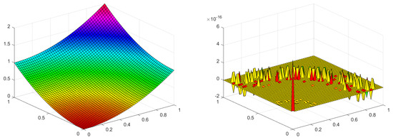
In Table 1, we compare the proposed method in the previous section with B-spline method [5]. Our method gives better results than the B-spline method. Figure 1 demonstrates the approximate solution on the left side and corresponding absolute errors on the right.

Table 1. Comparison between the proposed technique and the B-spline method [5] for Example 1.

		B-Spline Method [5]				Proposed Method
$\mathbf{J}$		3	4	5		3
$L^{\infty }$		$2.5\times {10}^{-2}$	$9.3\times {10}^{-3}$	$3.4\times {10}^{-3}$		$1.90\times {10}^{-14}$
$L^2$		$1.4\times {10}^{-2}$	$5.4\times {10}^{-3}$	$2.0\times {10}^{-3}$		$5.71\times {10}^{-15}$

Figure 1. Comparing the approximate and exact solutions, using $r=3$ and $J=2$, for Example 1.

Example 2.

We consider STFPDEs (1) where $a_1=a_2=1$, $\alpha =1/2$, $\beta =1/3$ and the function $f(x,t)$ is equal to

$$f(x,t)=\frac{t^2}{\sqrt{\pi }}\left(\mathcal{C}\left(\frac{\sqrt{2x}}{\sqrt{\pi }}\right)\sqrt{2\pi }cos\left(x\right)+\mathcal{S}\left(\frac{\sqrt{2x}}{\sqrt{\pi }}\right)\sqrt{2\pi }sin\left(x\right)\right)+\frac{9t^{5/3}sin\left(x\right)}{5\mathsf{\Gamma }(2/3)},$$

where $\mathcal{C}\left(x\right)$ and $\mathcal{S}\left(x\right)$ are the Fresnel integrals and are defined through the following power series,

$$\mathcal{C}\left(x\right)=\sum _{m=0}^{\infty }{(-1)}^m\frac{x^{4m+3}}{(2m+1)!(4m+3)},$$

and

$$\mathcal{S}\left(x\right)=\sum _{m=0}^{\infty }{(-1)}^m\frac{x^{4m+1}}{\left(2m\right)!(4m+1)}.$$

For this example, the exact answer is given as $w(x,t)=sin\left(x\right)t^2$.

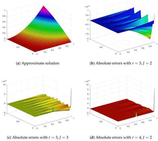
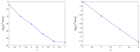
Table 2 shows the effect of the parameters r and J on the $L^2$-errors. It is evident that the error is reduced as parameters r and J tend to ∞. Figure 2 and Figure 3 illustrate the effect of J and r on the absolute errors and $L^2$-errors, respectively.

Table 2. Effect of the parameters r and J on $L^2$-errors at different times for Example 2.

r	J	$\mathit{t}=0.2$	$\mathit{t}=0.4$	$\mathit{t}=0.6$	$\mathit{t}=0.8$	$\mathit{t}=1.0$
3	2	$2.790\times {10}^{-6}$	$1.114\times {10}^{-5}$	$2.503\times {10}^{-5}$	$4.444\times {10}^{-5}$	$6.934\times {10}^{-5}$
	3	$2.891\times {10}^{-7}$	$1.165\times {10}^{-6}$	$2.635\times {10}^{-6}$	$4.703\times {10}^{-6}$	$7.370\times {10}^{-6}$
5	2	$6.244\times {10}^{-10}$	$2.479\times {10}^{-9}$	$5.542\times {10}^{-9}$	$9.801\times {10}^{-9}$	$1.524\times {10}^{-8}$
	3	$1.614\times {10}^{-11}$	$6.466\times {10}^{-11}$	$1.443\times {10}^{-10}$	$2.583\times {10}^{-10}$	$4.059\times {10}^{-10}$

Figure 2. Numerical results for Example 2.

Figure 3. Effect of the parameters r and J on $L^2$-errors for Example 2.

Example 3.

The third example is dedicated to the STFPDEs

$$\frac{{\partial }^{1/2}w(x,t)}{\partial x^{1/2}}+\frac{{\partial }^{1/3}w(x,t)}{\partial t^{1/3}}=\frac{15\sqrt{\pi }{x}^2{t}^2}{16}+\frac{9}{5\mathsf{\Gamma }\left(2/3\right)}{t}^{\frac{5}{3}}{x}^{\frac{5}{2}},$$

with conditions

$$w(x,0)=0,w(0,t)=0.$$

The exact solution for this equation is $w(x,t)=x^{5/2}{t}^2$.

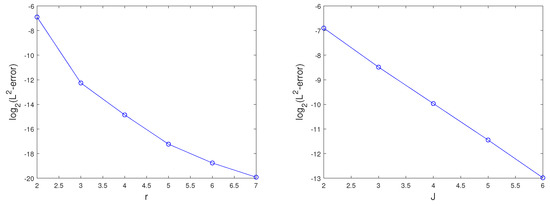
Table 3 shows the effect of the parameters r and J on the $L^2$-errors. It is evident that the error is reduced as parameters r and J tend to ∞. Figure 4 illustrates the effect of J and r on the $L^2$-errors, respectively.

Table 3. Effect of the parameters r and J on $L^2$-errors at different times for Example 3.

r	J	$\mathit{t}=0.2$	$\mathit{t}=0.4$	$\mathit{t}=0.6$	$\mathit{t}=0.8$	$\mathit{t}=1.0$
3	2	$1.781\times {10}^{-5}$	$7.199\times {10}^{-5}$	$1.631\times {10}^{-4}$	$2.914\times {10}^{-4}$	$4.570\times {10}^{-4}$
	3	$2.337\times {10}^{-6}$	$9.532\times {10}^{-6}$	$2.170\times {10}^{-5}$	$3.890\times {10}^{-5}$	$6.117\times {10}^{-5}$
5	2	$5.434\times {10}^{-7}$	$2.246\times {10}^{-6}$	$5.154\times {10}^{-6}$	$9.294\times {10}^{-6}$	$1.468\times {10}^{-5}$
	3	$7.152\times {10}^{-8}$	$2.965\times {10}^{-7}$	$6.814\times {10}^{-7}$	$1.230\times {10}^{-6}$	$1.944\times {10}^{-6}$

Figure 4. Effect of the parameters r and J on $L^2$-errors for Example 3.

5. Conclusions

Interpolating the scaling functions Tau method was proposed to solve the space–time fractional partial differential equations. According to the relation between the integral and derivative operators of the fractional order in the Caputo sense, we obtained the fractional derivative for ISFs as an operational matrix, indirectly. To this end, the operational matrices for the derivative operator and fractional integral were used. Using the Tau method, the considered equation was reduced to a system of algebraic equations. By solving this system, we found the approximate solution via an expansion based on interpolating scaling functions. We proved that the proposed method is convergent. Numerical results illustrated that the proposed method gives better results than other methods, and, in some cases, it is very accurate.

References

- Asadzadeh, M.; Saray, B.N. On a multiwavelet spectral element method for integral equation of a generalized Cauchy problem. BIT Numer. Math. 2022, 1–34. [Google Scholar] [CrossRef]
- Kilbas, A.; Srivastava, H.M.; Trujillo, J.J. Theory and applications of fractional differential Equations (24). In Theory and Applications of Fractional Differential Equations; Elsevier B.V.: Amsterdam, The Netherlands, 2006. [Google Scholar]
- Su, L.; Wang, W.; Xu, Q. Finite difference methods for fractional dispersion equations. Appl. Math. Comput. 2010, 216, 3329–3334. [Google Scholar] [CrossRef]
- Podlubny, I. Fractional Differential Equations; Academic Press: New York, NY, USA, 1999. [Google Scholar]
- Lakestani, L.; Dehghan, M.; Iroust-Pakchin, S. The construction of operational matrix of fractional derivatives using B-spline functions. Commun. Nonlinear Sci. 2012, 17, 1149–1162. [Google Scholar] [CrossRef]
- Mokhtary, P.; Ghoreishi, F.; Srivastavac, H.M. The Müntz-Legendre Tau method for fractional differential equations. Math. Comput. Simul. 2022, 194, 210–235. [Google Scholar] [CrossRef]
- Odibat, Z.; Momani, S.; Xu, H. A reliable algorithm of homotopy analysis method for solving nonlinear fractional differential equations. Appl. Math. Model. 2010, 34, 593–600. [Google Scholar] [CrossRef]
- Duan, J.S.; Rach, R.; Baleanu, D.; Wazwaz, A.M. A review of the Adomian decomposition method and its applications to fractional differential equations. Commun. Frac. Calc. 2012, 3, 73–99. [Google Scholar]
- Lin, Y.; Xu, C. Finite difference/spectral approximations for the time-fractional diffusion equation. J. Comput. Phys. 2007, 255, 1533–1552. [Google Scholar] [CrossRef]
- Saadatmandi, A.; Dehghan, M.; Azizi, M.R. The Sinc–Legendre collocation method for a class of fractional convection–diffusion equations with variable coefficients. Commun. Nonlinear Sci. Numer. Simul. 2012, 17, 4125–4136. [Google Scholar] [CrossRef]
- Odibat, Z.; Momani, S. A generalized differential transform method for linear partial differential equations of fractional order. Appl. Math. Lett. 2008, 21, 194–199. [Google Scholar] [CrossRef]
- Rida, S.Z.; El-Sayed, A.M.A.; Arafa, A.A.M. On the solutions of time-fractional reaction–diffusion equations. Nonlinear Sci. Numer. Simulat. 2010, 15, 3847–3854. [Google Scholar] [CrossRef]
- Chen, Y.; Wu, Y.; Cui, Y.; Wang, Z.; Jin, D. Wavelet method for a class of fractional convection–diffusion equation with variable coefficients. J. Comput. Sci. 2010, 1, 146–149. [Google Scholar] [CrossRef]
- Ray, S.S. Analytical solution for the space fractional diffusion equation by two-step adomian decomposition method. Commun. Nonlinear Sci. Numer. Simul. 2009, 14, 1295–1306. [Google Scholar]
- Saadatmandi, A.; Dehghan, M. A tau approach for solution of the space fractional diffusion equation. Comput. Math. Appl. 2011, 62, 1135–1142. [Google Scholar] [CrossRef]
- Dehghan, M.; Yousefi, S.A.; Lotfi, A. The use of He’s variational iteration method for solving the telegraph and fractional telegraph equations. Int. J. Numer. Biomed. Eng. 2011, 27, 219–231. [Google Scholar] [CrossRef]
- Dehghan, M.; Manafian, J.; Saadatmandi, A. Solving nonlinear fractional partial differential equations using the homotopy analysis method. Numer. Partial Differ. Equ. 2010, 26, 448–479. [Google Scholar] [CrossRef]
- Jiang, Y.; Ma, J. High–order finite element methods for time–fractional partial differential equations. J. Comput. Appl. Math. 2011, 235, 3285–3290. [Google Scholar] [CrossRef]
- Alpert, B.; Beylkin, G.; Coifman, R.R.; Rokhlin, V. Wavelet-like bases for the fast solution of second-kind integral equations. SIAM J. Sci. Stat. Comput. 1993, 14, 159–184. [Google Scholar] [CrossRef]
- Seyedi, S.H.; Saray, B.N.; Ramazani, A. On the multiscale simulation of squeezing nanofluid flow by a highprecision scheme. Powder Technol. 2018, 340, 264–273. [Google Scholar] [CrossRef]
- Saray, B.N. Abel’s integral operator: Sparse representation based on multiwavelets. BIT Numer. Math. 2021, 61, 587–606. [Google Scholar] [CrossRef]
- Saray, B.N. Sparse multiscale representation of Galerkin method for solving linear-mixed Volterra-Fredholm integral equations. Math. Methods Appl. Sci. 2020, 43, 2601–2614. [Google Scholar] [CrossRef]
- Saray, B.N.; Lakestani, M.; Dehghan, M. On the sparse multiscale representation of 2-D Burgers equations by an efficient algorithm based on multiwavelets. Numer. Meth. Part. Differ. Equ. 2021. [Google Scholar] [CrossRef]
- Afarideh, A.; Dastmalchi Saei, F.; Lakestani, M.; Saray, B.N. Pseudospectral method for solving fractional Sturm-Liouville problem using Chebyshev cardinal functions. Phys. Scr. 2021, 96, 125267. [Google Scholar] [CrossRef]
Publisher’s Note: MDPI stays neutral with regard to jurisdictional claims in published maps and institutional affiliations. |
© 2022 by the authors. Licensee MDPI, Basel, Switzerland. This article is an open access article distributed under the terms and conditions of the Creative Commons Attribution (CC BY) license (https://creativecommons.org/licenses/by/4.0/).