An Asymmetric Beamforming Method Based on Arithmetic Phase Difference Weighting in CSAMT

Abstract

Traditional controlled-source audio-frequency magnetotellurics (CSAMT) radiates symmetric beams using a grounded symmetric dipole (GSD). Only a tiny fraction of radiant energy is taken advantage of during the far-field (Ff) observation due to the low directivity of the GSD. In order to enhance the signal-to-noise ratio (SNR) during the Ff observation, it is necessary to reduce the transceiving distance (TD) or increase the transmitting power (TP), but both methods will cause many problems. Further, when using the tensor method for observation, GSDs in two vertical directions will be employed to radiate energy, and then a series of problems will occur such as an asymmetry of the SNR in two vertical directions if the geological conditions under the two GSDs vary widely. An arithmetic phase difference (APd) weighting asymmetric beamforming method (ABFM) in CSAMT is proposed in this paper, which uses a GSD array instead of a single GSD, and a signal with APd is transmitted to control the wavefront for beam steering. A significant enhancement (about 3 dB) of the SNR will occur by collecting the radiant energy in the region of concern (RoC) using ABFM. The analysis and simulation results demonstrate that under the premise of the same TD and TP, the ABFM has obvious advantages in improving energy utilization in CSAMT. In other words, the APd-weighted ABFM can deal with a complex noise environment in the field better than the traditional method.

1. Introduction

Controlled-source audio-frequency magnetotellurics (CSAMT) is a common electromagnetic prospecting method, which is mainly divided into the scalar method, vector method, and tensor method. Traditional scalar and vector CSAMT uses a grounded symmetric dipole (GSD) as a transmitting source. The symmetric dipole (SD) is one of the most straightforward antenna configurations that has a well-known symmetric radiation pattern. It can be realized with two metallic conductors that have a sinusoidal voltage difference applied between them. Due to the large transceiving distance (TD), the GSD should be treated as a point source with a symmetric radiation pattern. Significantly, when using the tensor method for observation, GSDs in two vertical directions will be employed to radiate energy. Because only a tiny fraction of the radiant energy from the GSD is utilized, while most of it is wasted, a shorter TD or higher transmitting power (TP) is necessary to generate an appropriate signal-to-noise ratio (SNR) at the receiving point. To enhance the SNR, traditional methods depend on increasing the TP or shortening the TD. On the one hand, due to the restriction of the current power electronics technology, the TP cannot be increased without limitation, and the higher the TP, the larger the weight and volume, which are not conducive to field exploration. On the other hand, shortening the TD will lead to some problems, such as the source effect that has been extensively studied by many scholars [1,2,3,4,5]. However, when the receiver is located in the near-field, the distortion of apparent resistivity or the impedance phase caused by the source effect will complicate the processing of CSAMT data and often leads to errors in inferring the underground geological structure.

The electromagnetic wave will deflect and refract during its propagation in the underground medium, so the vibration direction and phase of the electromagnetic wave will change. In scalar and vector CSAMT, the source is a single GSD. When the scalar and vector CSAMT detects the plane electromagnetic wave, it ignores the changes in the vibration direction, phase, and frequency of the electromagnetic wave, so it can only reflect the one-dimensional electrical structure. In most cases, it only establishes a unidirectional current vector underground, which can only measure $E_x,H_y$ (or $E_y,H_x$) (scalar method) and $E_x,E_y,H_x,H_y,H_z$ (vector method) components and then calculate the impedance.

A one-way current vector does not comprehensively mirror the relevant geological structure information when the geological conditions are relatively complex. When the electromagnetic wave propagates underground, the electrical property changes, not only along the vertical direction, but also along the trend, which is a two-dimensional electrical structure. When the electrical property changes in both horizontal and vertical directions, it is a three-dimensional electrical structure. $E_x$ and $E_y$ are induced not only by $H_y$ and $H_x$ but also by $H_x$ and $H_y$ depending on $Z_{xy}$ and $Z_{xx}$, respectively. According to the research results of tensor impedance [6], the definition of a two-dimensional electrical structure requires four electrical parameters, $Z_{xx},Z_{xy},Z_{yx}$ and $Z_{yy}$. The definition of the three-dimensional electrical structure requires nine electrical parameters, namely, $Z_{xx},Z_{xy},Z_{yx},Z_{xz},Z_{yy},Z_{yz},Z_{zx},Z_{zy}$ and $Z_{zz}$, where the electrical property is called tensor impedance. In the literature [7], the general calculation formula of magnetotellurics tensor impedance is derived; Equation (1) shows the three-dimensional tensor impedance relationship:

$$\left[\begin{array}{l}{E}_x\\ E_y\\ E_z\end{array}\right]=\left[\begin{array}{l}{Z}_{xx}{Z}_{xy}{Z}_{xz}\\ Z_{yx}{Z}_{yy}{Z}_{yz}\\ Z_{zx}{Z}_{zy}{Z}_{zz}\end{array}\right]\left[\begin{array}{l}{H}_x\\ H_y\\ H_z\end{array}\right]$$

(1)

Because the component of $E_z$ is very small, it is difficult to observe. In practice, the following tensor impedance expression (Equation (2)) is often used:

$$\left[\begin{array}{l}{E}_x\\ E_y\end{array}\right]=\left[\begin{array}{l}{Z}_{xx}{Z}_{xy}\\ Z_{yx}{Z}_{yy}\end{array}\right]\left[\begin{array}{l}{H}_x\\ H_y\end{array}\right]$$

(2)

After considering the magnetic transfer functions, we can obtain Equation (3):

$$\left[\begin{array}{l}{E}_x\\ E_y\\ H_z\end{array}\right]=\left[\begin{array}{l}{Z}_{xx}{Z}_{xy}\\ Z_{yx}{Z}_{yy}\\ T_{zx}{T}_{zy}\end{array}\right]\left[\begin{array}{l}{H}_x\\ H_y\end{array}\right]$$

(3)

where $E_x$, $E_y$ represent the electric field component (EFc) in the x, y directions; $H_x,H_y,H_z$ represent the magnetic field component (MFc) in the x, y, and z directions; $Z_{xx},Z_{xy},Z_{yx},Z_{yy}$ is the impedance tensor; $T_{zx}$, $T_{zy}$ are the magnetic transfer functions, and $T={\left[T_{zx}{T}_{zy}\right]}^T$ is the tilt vector.

When conducting three-dimensional detection, it is required to take the impedances of the above nine tensors. Obviously, it is necessary to monitor the electromagnetic field components (EMFc) in two directions, which requires the emission of two groups of electromagnetic fields that vary independently with different polarization directions. The tensor CSAMT employs GSDs with EMFc changing independently in two vertical directions; the GSDs in both directions can measure a total of ten components.

The first five EMFc received in the region of concern (RoC) are recorded as $E_{x1},E_{y1},H_{x1},H_{y1},H_{z1}$ (delegating the EFc in the x, y directions and the MFc in the x, y, and z directions of the GSD₁), and the last five EMFc are received and recorded as $E_{x2},E_{y2},H_{x2},H_{y2},H_{z2}$ in the same way. As shown in Equation (4) from the literature [7], six linear equations can be built from Equation (3) to acquire the tensor impedance and tilt vector. Thus, the sophisticated geological body with a three-dimensional structure can be explored.

$$\begin{array}{l}{Z}_{xx}=\frac{E_{x1}{H}_{y2}-E_{x2}{H}_{y1}}{H_{x1}{H}_{y2}-H_{x2}{H}_{y1}}{Z}_{yy}=\frac{E_{y1}{H}_{x2}-E_{y2}{H}_{x1}}{H_{x2}{H}_{y1}-H_{x1}{H}_{y2}}\\ Z_{xy}=\frac{E_{x2}{H}_{y1}-E_{x1}{H}_{x2}}{H_{x1}{H}_{y2}-H_{x2}{H}_{y1}}{Z}_{yx}=\frac{E_{y2}{H}_{y1}-E_{y1}{H}_{y2}}{H_{x2}{H}_{y1}-H_{x1}{H}_{y2}}\\ T_{zx}=\frac{H_{z1}{H}_{y2}-H_{z2}{H}_{y1}}{H_{x1}{H}_{y2}-H_{x2}{H}_{y1}}{T}_{zy}=\frac{H_{z2}{H}_{x1}-H_{z1}{H}_{x2}}{H_{x1}{H}_{y2}-H_{x2}{H}_{y1}}\end{array}$$

(4)

where $E_{x1},E_{y1},H_{x1},H_{y1},H_{z1}$ represent the EFc in the x, y directions and the MFc in the x, y, and z directions of the GSD₁; $E_{x2},E_{y2},H_{x2},H_{y2},H_{z2}$ represent the EFc in the x, y directions and the MFc in the x, y, and z directions of the GSD₂; $Z_{xx},Z_{xy},Z_{yx}$ and $Z_{yy}$ is the impedance tensor; $T_{zx}$, $T_{zy}$ are the magnetic transfer functions.

Although the use of tensor CSAMT for exploration can better identify three-dimensional geological bodies, when using the tensor method for observation, if the geological conditions under the two GSDs vary widely, a series of problems will occur such as the asymmetry of the SNR in two vertical directions, i.e., an obvious feeble region in each component within the exploration area. When we utilize CSAMT for exploration, no matter how different the geological conditions are, we hope to maximize the use of radiant energy during the Ff observation to allow for high-quality data acquisition. Therefore, in order to improve the SNR in RoC, this paper introduces an asymmetric beamforming method (ABFM) based on arithmetic phase difference (APd) weighting in CSAMT, which maximizes the main lobe energy, reduces the sidelobe energy to an acceptable level, and achieves the required beam steering capability that traditional methods often cannot provide.

2. Principle and Methods of ABFM

The pattern of each unit in the antenna array is structurally in conjunction with the adjacent units to shape a main lobe, which radiates energy in the required direction. Generally speaking, in the normalized pattern, the maximum amplitude of the main lobe is 1, and the radiation lobes on both sides that are separated from the main lobe and have low amplitude are called side lobes. These radiations do not contribute to the radiation in the main direction. Therefore, it is always hoped that the lower, the better. The original intention of the antenna optimization is to suppress side lobes to a low level and guide the effective beam to point to the RoC. The array signal processing method is to achieve beam control by modulating the phase or amplitude of the signal. The ABFM in this paper is mainly used to control the phase of the array signal. A directional asymmetric beam can be shaped to improve energy utilization and achieve beam steering by adjusting the phase difference (Pd) weighting coefficient of each unit in the antenna array.

To achieve ABFM, the source needs to employ a GSD array rather than a single GSD because the beam of a single GSD is diffused in a spherical style and cannot be manually intervened, which is called the symmetric beamforming method (SBFM) in this paper. As for the antenna array, many scholars have conducted research in many fields, such as aerospace [8,9]; multi-channel GPR surveys [10]; the improvement of SNR and the penetration depth of phased arrays [11,12]; and the optimization of the location accuracy of three dimensional (3D) objects [13,14,15,16,17,18,19].

The two GSDs are placed along the y-axis with a certain spacing $d$, and the current direction of the two GSDs is along the x-axis, as depicted in Figure 1. Assuming that the electromagnetic field between two GSDs is uncoupled, the global radiation is the sum of the field intensity vectors of the two GSDs [20]. All array units are excited with the same voltage and different phases; then, the steering of the main lobe is guided by the APd values, that is, the deflection angle $\theta$ has a linear correlation with the APd values. If the weighting coefficient of each array unit can be properly regulated according to the exploration conditions, the signal strength in the required direction can be enhanced as much as possible and the radiation in the unexpected direction can be weakened. That is, ABFM has been implemented because the beam points to the RoC.

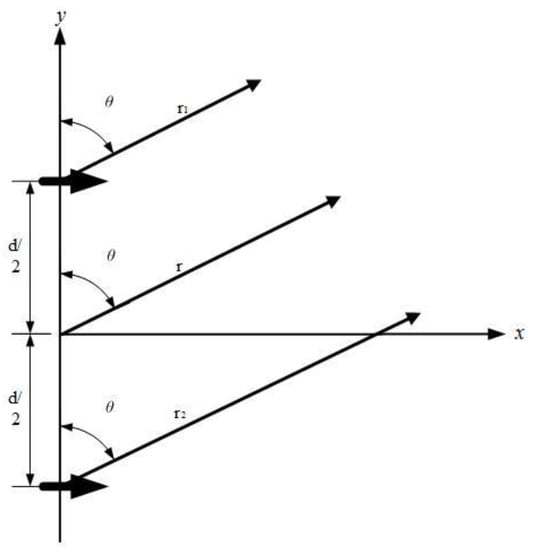
Figure 1. Two GSDs placed along the y-axis with a certain spacing d during the Ff observations with the same magnitude and different phases.

Where $\theta$ is the angle between the line formed by the base point and the Ff point and the y-axis; $d$ is the distance between two GSDs; $r$ is the distance from the Ff point to the GSDs.

It goes without saying that the two GSDs are arranged in a line along the y-axis, assuming that each unit has the same magnitude and a different phase (the phase of one unit is ahead of the adjacent one by a Pd $\beta$). Some researchers [21] had provided the solution for the EFc radiated by a single GSD whose direction of current was along the x-axis. During the near-field observations, we obtain the following:

$$E_{\theta }\cong -j\eta \frac{I_{0}l{e}^{-jkr}}{4\pi k{r}^3}\cos \theta$$

(5)

$$E_r\cong -j\eta \frac{I_{0}l{e}^{-jkr}}{2\pi k{r}^3}\sin \theta ,\mathrm{wherein},kr\ll 1$$

(6)

When observing the middle of the field, it can be concluded that

$$E_{\theta }\cong -j\eta \frac{k{I}_{0}l{e}^{-jkr}}{4\pi r}\cos \theta$$

(7)

$$E_r\cong \eta \frac{I_{0}l{e}^{-jkr}}{2\pi r^2}\sin \theta ,\mathrm{wherein},kr>1$$

(8)

During Ff observation, it can be inferred that

$$E_{\theta }\cong j\eta \frac{k{I}_{0}l{e}^{-jkr}}{4\pi r}\cos \theta$$

(9)

$$E_r\cong 0,\mathrm{wherein},kr\gg 1$$

(10)

where $E_{\theta }$ and $E_r$ represent the EFc radiated by a single GSD, $r$ is the distance from the observation point to the GSD, $\theta$ is the angle between the line formed by the base point and the observation point and the y-axis, $\eta$ is wave impedance, $k$ is the wave number, $l$ is the distance between two GSDs, and $I_0$ is the current distribution on the GSD.

When the voltage magnitudes of the two GSDs are equal and there is a specific Pd $\beta$ between the adjacent units, during the Fr observation, due to the same direction, the field values of two GSDs should be added directly.

$$E_t=E_{GS{D}_1}+E_{GS{D}_2}=\theta j\eta \frac{I_{0}l}{4\pi }\left[\frac{e^{-j\left[k{r}_1-\frac{\beta }{2}\right]}}{r_1}\cos {\theta }_1+\frac{e^{-j\left[k{r}_2-\frac{\beta }{2}\right]}}{r_2}\cos {\theta }_2\right]$$

(11)

From the Ff assumption in Figure 1, we can conclude that

$$r_1\cong r-\frac{d}{2}\cos \theta ,r_2\cong r+\frac{d}{2}\cos \theta$$

(12)

Substitute the above Equation (12) into Equation (11) and extract the common factor to obtain the following:

$$\begin{array}{l}{E}_t=\theta j\eta \frac{I_{0}l{e}^{-jkr}}{4\pi r}\cos \theta \left[e^{j(kd\cos \theta +\beta )/2}+e^{-j(kd\cos \theta +\beta )/2}\right]\\ =\theta j\eta \frac{I_{0}l{e}^{-jkr}}{4\pi r}\cos \theta \left\{2\cos \left[\left(kd\cos \theta +\beta \right)/2\right]\right\}\end{array}$$

(13)

Because the units of the array are consistent, the unit can be treated as a point source when calculating the array factor $AF$. The pattern can be estimated by multiplying $AF$ by the Ff of one unit. After normalization, we obtain the following:

$$A{F}_n=\cos \left[\left(kd\cos \theta +\beta \right)/2\right]$$

(14)

As can be seen from Equation (15), the array can control the characteristics of $AF$ and field density by adjusting the spacing or phase between units. When $N$ GSDs are arranged in a line along the y-axis, assuming that each unit has the same voltage magnitude and different phases, the $AF$ is

$$\begin{array}{l}AF=1+e^{+j(kd\cos \theta +\beta )}+e^{+j2(kd\cos \theta +\beta )}+\dots +e^{+j(N-1)(kd\cos \theta +\beta )}\\ ={\displaystyle \sum _{n=1}^N{e}^{j(n-1)(kd\cos \theta +\beta )}}={\displaystyle \sum _{n=1}^N{e}^{j(n-1)\psi }}\end{array}$$

(15)

When $\psi =kd\cos \theta +\beta$, it can be obtained by referring to the summation equation $S=a_1\frac{1-q^n}{1-q}$:

$$\begin{array}{l}AF=\frac{e^{jN\psi }-1}{e^{j\psi }-1}\\ =e^{j\left[\left(N-1\right)/2\right]\psi }\left[\frac{e^{j\left(N/2\right)\psi }-e^{-j\left(N/2\right)\psi }}{e^{j\left(1/2\right)\psi }-e^{-j\left(1/2\right)\psi }}\right]=e^{j\left[\left(N-1\right)/2\right]\psi }\left[\frac{\sin \left(N\psi /2\right)}{\sin (\psi /2)}\right]\end{array}$$

(16)

If the array center is the base point, the $AF$ can be simplified to

$$AF=\frac{\sin \left(N\psi /2\right)}{\sin (\psi /2)}$$

(17)

When $\psi$ approaches 0, Equation (18) can be obtained as follows:

$$\underset{\psi \to 0}{\lim }\frac{\sin \left(N\psi /2\right)}{\sin (\psi /2)}=N$$

(18)

Then, the $AF$ after normalization is

$$A{F}_n=\frac{\sin \left(N\psi /2\right)}{N\sin (\psi /2)}$$

(19)

It is known that the ${\theta }_m$ of the array is in the range of 0–180°; referring to Equation (19), when $\psi /2=0$, $AF$ has the maximum value, and we can calculate the angle ${\theta }_m$ of the main lobe.

$$\frac{1}{2}\psi =\frac{kd\cos {\theta }_m+\beta }{2}=\pm n\pi ,n=0$$

(20)

$${\theta }_m={\cos }^{-1}\left[\frac{-\beta \pm 2n\pi }{kd}\right],n=0$$

(21)

Finally, we can draw a conclusion as shown in Equation (22), and then ABFM can be realized.

$${\theta }_m={\cos }^{-1}\left[\frac{-\beta }{kd}\right]$$

(22)

3. SBFM and ABFM Simulation of SD

Figure 2 shows the 1 × 2 SD arrays placed parallel in the air at a certain distance. Assuming that there is only one single SD in Figure 2, when the EFc is observed at the same polarization from all angles, the radiant energy attenuation is isotropic, that is, there is no directivity. Assume that another SD with same phase is added and the two SDs are separated by a specific distance. Even if the positions of the two SDs are different, the absolute values of the EMFc signals at two positions symmetrical to the centerlines of the two SDs are the same, so the signals lack directivity. In both cases, the EMFc generated by the source is symmetric.

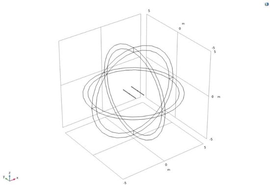
Figure 2. 1 × 2 SD arrays are placed in the air in parallel at a certain distance apart.

However, if another SD with different phases is added, and the two SDs are kept at a specific spacing, and intervention will come into being between the two wave trains, which means that the magnitude will increase in some directions and decrease in other directions.

3.1. SBFM Simulation of SD

As shown in Figure 2, the space of the model is the air domain with ${\epsilon }_r=1$, ${\mu }_r=1$ and $\sigma =0S{m}^{-1}$, and the free space wavelength at the SD’s operating frequency is 4 m. Thus, the SD arms are 1 m long and are aligned with the y-axis. The arm radius is chosen to be 0.05 m. The 1 × 2 SD arrays are excited with AC voltage signals of the same frequency, amplitude, and phase, which are placed in the air in parallel with an interval of 1 m. Figure 3b shows that the polar plot of the Ff pattern in the xz-plane is isotropic.

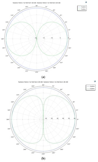
Figure 3. The polar plot of the Ff pattern in the xz-plane is isotropic. (a) Ff pattern of a single SD. (b) Ff pattern of a 1 × 2 SD array.

Relatively speaking, assuming that there is only one single SD in Figure 2, when the EFc is observed at the same polarization from all angles, the radiant energy attenuation is also isotropic, as shown in Figure 3a.

The polar plot in Figure 3 of the Ff pattern in the xz-plane shows the isotropic radiation pattern. The 3D visualization of the Ff intensity in Figure 4 shows the symmetric pattern.

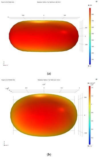
Figure 4. A 3D visualization of the Ff pattern of the SD shows the symmetric pattern. (a) Ff pattern of a single SD. (b) Ff pattern of a 1 × 2 SD array.

3.2. ABFM Simulation of SD

Consistent with the settings in Figure 2, the 1 × 2 SD arrays are excited with AC voltage signals of the same frequency and amplitude but a different phase (the excitation phase of SD₁ is 90 degrees ahead of the phase of SD₂) and are placed in the air in parallel with an interval of 1 m. The polar plot in Figure 5 of the Ff pattern in the xz-plane shows the anisotropic radiation pattern.

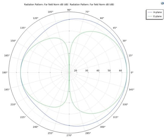
Figure 5. The polar plot of the Ff pattern in the xz-plane is anisotropic.

The 3D visualization of the Ff intensity in Figure 6 shows the expected asymmetric pattern. It can be seen that the beam deflects towards the SD with a phase lag.

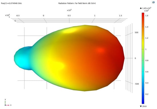
Figure 6. A 3D visualization of the Ff pattern of the 1 × 2 SD array shows the expected asymmetric pattern.

4. ABFM Simulation in CSAMT

Figure 7 shows the traditional 1 × 1 CSAMT, 1 × 2 GSD array CSAMT, and GSD array tensor measurement CSAMT models, which are sphere models with a radius of 10 km. The upper half-space of the models is the air domain, of which the parameter settings are consistent with those in Figure 2. The lower half-space of the models is the soil domain with ${\epsilon }_r=2$, ${\mu }_r=1$, and $\sigma =0.01S{m}^{-1}$. In Figure 7a, a 1 × 1 GSD model with a 2 km length, a 0.04 m radius, and a 0.1 m gap between the two conductors is depicted. Figure 7b shows a 1 × 2 GSD array with two GSDs separated by 1 km placed along the y-axis on the ground, and other parameters are the same as those in Figure 7a. The GSD array tensor measurement CSAMT model is shown in Figure 7c, whose half-space and GSD parameters are consistent with the settings in Figure 7a. The two GSDs of the tensor measurement CSAMT are placed on the two corners of an isosceles triangle with an edge of 8 km, which can ensure that the measurement point is located in the Ff.

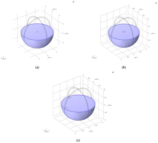
Figure 7. (a) Traditional 1 × 1 CSAMT model. (b) 1 × 2 GSD array CSAMT model. (c) GSD array-separated tensor CSAMT model.

4.1. Simulation Results of APd-Weighted ABFM Based on the 1 × 2 GSD Array CSAMT Model

According to the settings in Figure 7b, the 1 × 2 GSD arrays were given AC signal excitations with the same amplitude but different phases. The Pd between each GSD is related by a specific law, which is used to guide the steering of the main lobe. The asymmetric beam steering ability of the 1 × 2 GSD array can be acquired by running a phase (ph) scan. The ph of GSD₁ is 0 deg, and that of GSD₂ changes from −90 to 90 deg, varying every 30 deg. Figure 8 shows the symmetric beam is focused on the central axis without deflection when the 1 × 2 GSD arrays were given excitations with the same phases (0 deg) and voltage (800 V).

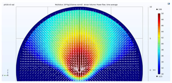
Figure 8. Amplitude of the E-plane EFc and Poynting vector direction when symmetry occurs.

Figure 9 illustrates the 1 × 2 GSD array placed along the y-axis, exciting the same amplitude (800 V) but different phases. For a special example, when the ph of GSD₁ is 0 deg and that of GSD₂ is −90 deg, the beam is deflected towards GSD₂ because the ph of GSD₂ lags behind that of GSD₁. On the contrary, when the ph of GSD₂ is ahead of that of GSD₁, the beam will steer towards GSD₁.

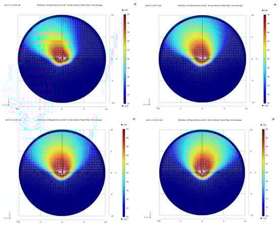
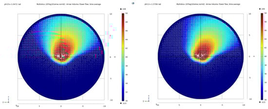
Figure 9. Amplitude of the E-plane EFc and Poynting vector direction when asymmetry occurs. The 1 × 2 GSD arrays were given excitations with the same voltage (800 V) but different phases; the ph of GSD₁ is 0 deg and that of GSD₂ changes from −90 to 90 deg, varying every 30 deg.

The asymmetric phenomenon is displayed as the E/H-plane multifaceted integration, as shown in Figure 10, and the beam has varying deflection under different Pds. The larger the Pd, the greater the deflection angle. The beam can be adjusted to steer to the RoC by adjusting the Pd. When the 1 × 2 GSD arrays are excited with the same amplitude and phase, the beam propagates symmetrically along the central axis of two GSDs (wathet), and the asymmetric beam steering can be achieved by adjusting the APd (other colors).

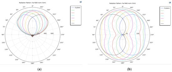
Figure 10. (a) E-plane pattern multifaceted integration and (b) H-plane pattern multifaceted integration. The 1 × 2 GSD arrays were given excitations with different phases and the same amplitude (800 V); the ph of GSD₁ was 0 deg and that of GSD₂ changed from −90 to 90 deg, varying every 30 deg.

A properly optimized 1 × 2 GSD array CSAMT should have a higher main lobe and lower side lobe levels, which is not obvious when plotted on a polar plot. The 3D Ff pattern (Figure 11) makes the ratio of the main lobe and side lobes more visible.

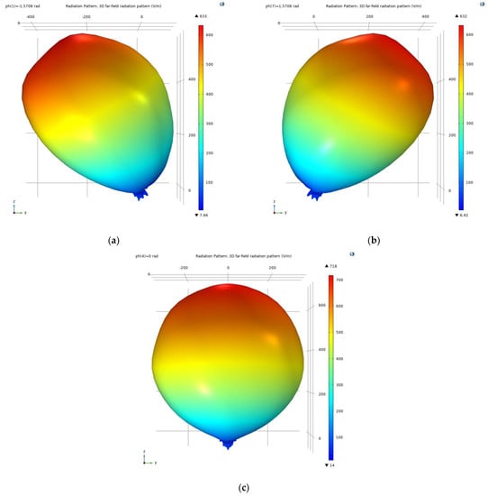
Figure 11. 3D Ff pattern. (a) ph = −90 deg. (b) ph = 90 deg. (c) ph = 0 deg.

All of the above simulation results indicate that the application of APd-weighted ABFM is effective. In the 1 × 2 GSD array CSAMT, the beam can be steered to the RoC through different phase excitations. Compared to the non-directional radiation of a single GSD, the SNR received by the receiving point in the RoC can be effectively improved.

4.2. Simulation Results of APd-Weighted ABFM Based on the GSD Array Separated Tensor CSAMT Model

As mentioned earlier, if another GSD is added and the two GSDs are kept at a specific interval, intervention will come into being between the two wave trains, which means that the magnitude will increase in some directions and decrease in other directions. The half-space and 1 × 2 GSD array tensor measurement CSAMT model was set up according to the model shown in Figure 7c. Figure 12 shows a 1 × 2 GSD array tensor measurement CSAMT model placed on the two corners of an isosceles triangle with an edge of 8 km. Electromagnetic interference phenomenon can occur under the excitation of the same phase and amplitude using traditional methods. When the excitation of two GSDs is in phase, under the influence of interference, the symmetric radiation energy flow is divided into multiple beams symmetrically distributed along the red line in the figure.

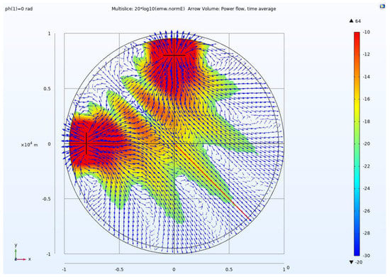
Figure 12. The excitations of two GSDs in phase (0 deg), the symmetric EFc distribution with intervention, and the Poynting vector direction; the red line shows the center line position.

Generally speaking, the receiving point is typically located at the center position during the separation tensor CSAMT, as depicted in Figure 13. At this location, the energy density is greater than that at other points, and the SNR of each EMFc in both directions is also higher and more symmetrical. Therefore, the tensor impedance calculated using the six linear equations mentioned above is more accurate.

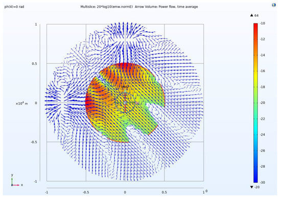
Figure 13. Receiving point position (SNR of EMFc in both directions at this position is higher and more symmetrical).

According to the above analysis, when the 1 × 2 GSD arrays are excited by different phases, the beam will deflect. The asymmetric beam steering ability of the 1 × 2 GSD array can be acquired by running a ph scan. Figure 14 illustrates the 1 × 2 GSD array tensor measurement CSAMT model that is excited by different phases. The port ph of GSD₁ is 0 deg and that of GSD₂ changes from −120 to 120 deg. With the phase change of GSD₂, multiple beams are gradually scanned, which provides an opportunity to compensate for the differences caused by different geological conditions.

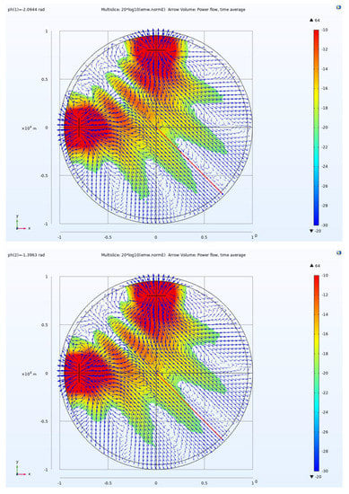
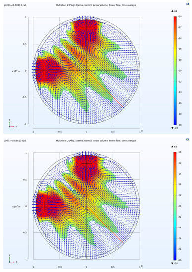
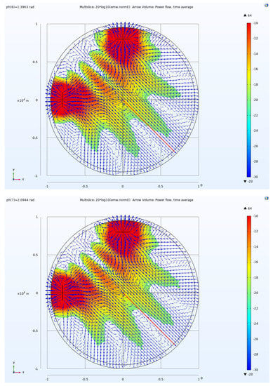
Figure 14. The excitations of the two GSDs in different phases, the asymmetric EFc distribution with intervention, and the Poynting vector direction; the red line shows the center line position. The port ph of GSD₁ is 0 deg and that of GSD₂ changes from −120 to 120 deg, varying every 40 deg.

5. Discussion

5.1. Comparative Discussion of the 1 × 2 GSD Array and Traditional 1 × 1 CSAMT

Compared to a single GSD in CSAMT, the 1 × 2 GSD array will achieve beam steering by changing the phase difference and will thus realize the concentration of electromagnetic energy in RoC. It is assumed that the power in both cases is 40 kW; on the premise of the same TP and TD, through the application of APd-weighted ABFM, the signals received in the RoC have a higher magnitude than those in the traditional method. Table 1 depicts the excitation of two source modes with the same power.

Table 1. Excitation of two source modes under the same power.

Source Mode	Voltage (V)	Current (A)	Phase (deg)	Total Power (kW)
1 × 2 GSD array	GSD1 800	25	0	40
	GSD2 800	25	90
Single GSD	1000	40	0	40

Based on Table 2, when the two exploration methods are implemented at different receiving points (the TD ranges from 5 km to 8 km and the measurement is conducted every 1 km), the EFc value generated by the 1 × 2 GSD array is about twice that of the single GSD during the Ff observation.

Table 2. Comparison of the EFc norm normalized according to the TP and TD.

Position (X, Y, Z)	V/m of 1 × 2 GSD Array	V/m of Single GSD
(0, −8000, 0)	12.229 × 10−13	5.484 × 10−13
(0, −7000, 0)	14.278 × 10−13	7.297 × 10−13
(0, −6000, 0)	19.584 × 10−13	10.394 × 10−13
(0, −5000, 0)	28.428 × 10−13	13.296 × 10−13

According to the SNR calculation formula $S=10\lg \frac{P_s}{P_n}$, assuming that the effective power received by the receiver is $P_{sg}$ when a single GSD is applied, then the effective power received when the GSD array is applied is about $2P_{sg}$, and the noise power $P_n$ of both is equal. Then, we can obtain the following:

$$S_{sg}=10\lg \frac{P_{sg}}{P_n}$$

(23)

$$S_{ay}=10\lg \frac{2P_{sg}}{P_n}$$

(24)

where $S_{sg}$ represents the SNR received by the receiver when a single GSD is applied; $S_{ay}$ represents the SNR received by the receiver when a GSD array is applied.

By subtracting Equation (24) from Equation (23), the difference between their SNR values is about 3 dB. In other words, the SNR of the GSD array is better than that of the conventional method (3 dB), which has obvious advantages in dealing with a complex noise environment in the field.

5.2. Comparative Discussion of APd-Weighted ABFM and Traditional Methods Based on the Separated Tensor CSAMT Model

As mentioned earlier, the receiving point is typically located at the center position during the separation tensor CSAMT; at this location, the energy density is greater than that at other points, and the SNR of each EMFc in both directions is also higher and more symmetrical. However, the main energy beam deviates frequently from the center position during actual exploration due to the heterogeneity of the earth. As a result, the SNR is often reduced when receiving at the center position. When APd-weighted ABFM is applied, the main energy beam will rotate around the origin within a certain range, similar to the pointer of a clock with the APd weighting running. For this reason, there will always be a time when the main beam will cover the center position, even if the earth is heterogeneous.

In the actual tensor measurement CSAMT exploration process, the receiver can be placed in the center, and then the APd-weighted ABFM can be used for beam steering. When the SNR at the receiving point is the strongest, the corresponding phase can be saved and applied to the subsequent tensor measurement CSAMT. Due to this, the EMFc and SNR of the two directions are more balanced than in the traditional method. There is no strong or weak EFc in the entire receiving point. In this way, the calculated tensor impedance is more accurate after the six linear equations are established.

6. Conclusions

Herein, an asymmetric beamforming method based on arithmetic phase difference weighting in CSAMT is proposed, which uses a GSD array instead of a single GSD, and a signal with APd is transmitted to control the wavefront for beam steering. A significant enhancement (about 3 dB) of the SNR will occur by collecting the radiant energy in the RoC using ABFM. The analysis and simulation results demonstrate that under the premise of the same TD and TP, the ABFM has obvious advantages in improving energy utilization in CSAMT. In other words, using the APd-weighted ABFM can deal with a complex noise environment in the field better than the traditional method.

Firstly, the principle and methods of ABFM are presented. Furthermore, the SBFM and ABFM of SD are simulated. Then, on the basis of the aforementioned calculations and analysis of APd-weighted ABFM, several numerical models for the application of ABFM with analytical solutions in CSAMT are built. Finally, the effect of APd-weighted ABFM is compared with that of conventional methods. The theoretical analysis and simulation results were all consistent, verifying the correctness and effectiveness of the proposed APd-weighted ABFM in CSAMT.

References

- Chen, M.S.; Yan, S. Research on the analysis for the copy effect of the field area, recording rule, shadow and field source in CSAMT exploration. Chin. J. Geophys. 2005, 48, 951–958. (In Chinese) [Google Scholar] [CrossRef]
- Tang, J.T.; Ge, W.N. Shadow and additional effect of the field source in 3D CSAMT. Comput. Tech. Geophys. Geochem. Explor. 2012, 34, 19–26. [Google Scholar]
- Shlykov, A.A.; Saraev, A.K. Wave effects in the field of a high frequency horizontal electric dipole. Izv.-Phys. Solid Earth 2014, 50, 249–262. [Google Scholar] [CrossRef]
- Lei, D.; Wu, X.P.; Di, Q.Y.; Wang, G.; Lv, X.G.; Wang, R.; Yang, J.; Yue, M.X. Modeling and analysis of CSAMT field source effect and its characteristics. J. Geophys. Eng. 2016, 13, 49–58. [Google Scholar]
- Luo, W.; Wang, X.B.; Wang, K.P.; Zhang, G.; Li, D.W.; Yang, Y.H. Study on the characteristics of magnetotelluric source effects and its correction. Chin. J. Geophys. 2021, 64, 2952–2964. [Google Scholar]
- Wang, X.X.; Di, Q.Y.; Xu, C. Characteristics of Multiple Dipole Sources and Tensor Measurement in CSAMT. J. Geophys. 2014, 57, 651–661. [Google Scholar]
- Tan, H.D.; We, W.B.; Deng, M.; Jin, S. General calculation formula of magnetotelluric tensor impedance. Oil Geophys. Prospect. 2004, 39, 113–116. [Google Scholar]
- Pozar, D.M. A relation between the active input impedance and the active unit pattern of a phased array. IEEE Trans. Antennas Propag. 2003, 51, 2486–2489. [Google Scholar] [CrossRef]
- Zhao, Y.; Zhang, Q.; Tang, B. Frequency diversity array MIMO track-before-detect in coherent repeated interference. IEICE Transactions on Fundamentals of Electronics. Commun. Comput. Sci. 2018, 10, 1703–1707. [Google Scholar]
- Lutz, P.; Perroud, H. Phased-array transmitters for GPR surveys. J. Geophys. Eng. 2006, 3, 35–42. [Google Scholar] [CrossRef]
- Garambois, S.; Senechal, P.; Perroud, H. On the use of combined geophysical methods to assess water content and water conductivity of near-surface formations. J. Hydrol. 2002, 259, 32–48. [Google Scholar] [CrossRef]
- Liu, X.S.; Zhou, F.; Zhou, H.; Tian, X.; Jiang, R.X.; Chen, Y.W. Parallel subarray beamforming algorithm based on cross array. Journal of Jilin University. Eng. Technol. Ed. 2016, 46, 1330–1336. [Google Scholar]
- Lehmann, F.; Boerner, D.E.; Holliger, K.; Green, A.G. Multicomponent georadar data: Some important implications for data acquisition and processing. Geophysics 2000, 65, 1542–1552. [Google Scholar] [CrossRef]
- Radzevicius, S.J.; Daniels, J.J.; Guy, E.D.; Vendl, M.A. Significance of crossed-dipole antennas for high noise environments. In Proceedings of the 13th EEGS Symposium on the Application of Geophysics to Engineering and Environmental Problems, Arlington, VA, USA, 20–24 February 2000; pp. 407–413. [Google Scholar] [CrossRef]
- Yarovoy, A.G.; Ligthart, L.P. Full-polarimetric video impulse radar for landmine detection. In Proceedings of the 2nd International Workshop on Advanced Ground Penetrating Radar, Delft, The Netherlands, 14–16 May 2003; Volume 1, pp. 246–250. [Google Scholar]
- Lutz, P.; Garambois, S.; Perroud, H. Influence of antenna configurations for GPR survey: Information from polarization and amplitude versus offset measurements Ground Penetrating Radar in Sediments. Geol. Soc. Lond. 2003, 211, 299–313. [Google Scholar] [CrossRef]
- Moran, M.L.; Greenfield, R.J.; Arcone, S.A. Modeling GPR radiation and reflection characteristics for a complex temperate glacier bed. Geophysics 2003, 68, 559–565. [Google Scholar] [CrossRef]
- Kraus, D.; Lemor, R.M. High Frequency 3D-Sonar Imaging for the Inspection of Underwater Constructions. In Proceedings of the 8th European Conference on Synthetic Aperture Radar, Aachen, Germany, 7–10 June 2010. [Google Scholar]
- Josserand, T.; Wolley, J. A miniature high resolution 3-D imaging sonar. Ultrasonics 2011, 51, 275. [Google Scholar] [CrossRef] [PubMed]
- Hu, Y.; Han, L.G.; Wu, R.S.; Xu, Y.Z. Multi-scale time-frequency domain full waveform inversion with a weighting local correlation-phase misfit function. J. Geophys. Eng. 2019, 16, 1017–1031. [Google Scholar] [CrossRef]
- Fan, H.F.; Zhang, Y.M.; Wang, X.H. A novel phased-array transmitting source in controlled-source audio-frequency. J. Geophys. Eng. 2022, 19, 595–614. [Google Scholar] [CrossRef]
Publisher’s Note: MDPI stays neutral with regard to jurisdictional claims in published maps and institutional affiliations. |
© 2022 by the authors. Licensee MDPI, Basel, Switzerland. This article is an open access article distributed under the terms and conditions of the Creative Commons Attribution (CC BY) license (https://creativecommons.org/licenses/by/4.0/).