Abstract
In this investigation, two different models for two coupled asymmetrical oscillators, known as, coupled forced damped Duffing oscillators (FDDOs) are reported. The first model of coupled FDDOs consists of a nonlinear forced damped Duffing oscillator (FDDO) with a linear oscillator, while the second model is composed of two nonlinear FDDOs. The Krylov–Bogoliubov–Mitropolsky (KBM) method, is carried out for analyzing the coupled FDDOs for any model. To do that, the coupled FDDOs are reduced to a decoupled system of two individual FDDOs using a suitable linear transformation. After that, the KBM method is implemented to find some approximations for both unforced and forced damped Duffing oscillators (DDOs). Furthermore, the KBM analytical approximations are compared with the fourth-order Runge–Kutta (RK4) numerical approximations to check the accuracy of all obtained approximations. Moreover, the RK4 numerical approximations to both coupling and decoupling systems of FDDOs are compared with each other.
1. Introduction
Nonlinear differential equations of the second- and third-order have attracted great attention from many researchers due to their many applications in various fields of science especially in engineering problems and in modeling robotics motion [1,2]. For instance, the Duffing equation (DE) is a second-order differential equation, which has spread widely due to its many applications in physics, chemistry, and in modeling many engineering problems [3,4]. It is typically regarded as a paradigm for nonlinear dynamics of dissipative systems. The Duffing equation (DE)/Duffing oscillator (DO) has been used successfully to describe and model a variety of physical and chemical processes, and several engineering problems, such as reinforcing springs, beam buckling, nonlinear electronic circuits, among others [3]. Given a physical system that has some form of potential energy associated with it, its dynamics in the neighborhood of a potential minimum can always be approximated by a linear oscillator. The oscillator restorative force coefficient incorporates the curvature of the potential well and is the first term of the Taylor series in which it can develop the position-dependent force acting on the already mentioned physical system. Taking more terms of the series improves the approximation. The next term of the Taylor series that brings about qualitative changes is the one that goes with the cube of the position (the quadratic term only implies a change in the equilibrium position). Narasimha [5] stated the general equations of the dynamics of a thin wire. The center point of a vibrating wire whose ends are embedded can be described as a one-dimensional effective oscillator. It was shown that for this oscillator the cubic term should not be neglected under resonance conditions. The micro clamped–clamped oscillator should share this characteristic with the vibrating wire as it is also a thin body tensed between anchors, therefore, its dynamics are governed by the following forced damped Duffing oscillator (FDDE)
where m represents the pendulum mass, gives the coefficient of the damping force (damping parameter), and k denotes the effective stiffness constant while f and indicate the amplitude and frequency of the driving force. The new term is , which represents the nonlinear relationship of the increase in the restoring force as the tension in the beams increases due to their elongation. Again, the equation is dimensionless. The unit of time is and the position is . There are now two free parameters, namely, and , defined by
with and , where indicates the normalized friction coefficient and represents the coefficient of the nonlinear term. It is considered that these are the two parameters that define the system. We want to find the motion of the oscillator when it is excited with frequency .
One of the desirable properties of a clock-like oscillator is that it has a stable frequency. The linear oscillator has a stable frequency near the resonance maximum, but the DO loses that property, particularly when fluctuations in amplitude affect the frequency of the system. The dependency of the frequency on the phase has a promising local maximum (zero slope), but according to the range in which frequency fluctuations can be tolerated, it may not be enough.
What can be interpreted from the measurements is that micro-oscillators behave as coupled Duffing oscillators (DOs) with another higher-frequency oscillator. In the current investigation, we propose a model consisting of a nonlinear oscillator that experiences a forced external coupling and a coupling due to the second oscillator. This second oscillator is linear and sustains its movement only by coupling with the main oscillator. The dynamics of this system can be modeled by the pair of equations
The two oscillators have different natural frequencies (given by the ratio ). The width of their resonance curves is given by . The coupling, in principle, is asymmetric due to . The system (3) may be rewritten in the following initial-value problem (i.v.p.) form, known as, coupled forced damped Duffing oscillators (FDDOs)
with the initial conditions (ICs)
where , , , , , , , and . We assume that the coupling is weak, that is, and .
Furthermore, in our investigation, we try to find an explicit approximation to the following coupled FDDOs [6]
with the ICs
where indicate the damping coefficients of both first and second oscillators, represent the driving forces, express the linear coupling stiffness parameters, denote the linear stiffness parameters, and represent the parameters of nonlinear terms. Furthermore, represent any time-dependent functions.
Some studies have been conducted around coupled Duffing-type oscillators [7,8,9,10,11,12], but an explicit solution to the coupled Duffing-type oscillators is rarely found in the published papers. In our study, we use the Krylov–Bogoliubov–Mitropolsky (KBM) method [7,8,9] for analyzing the two models of coupled FDDO including the first model (4) and the second model (6). The proposed method is successful in analyzing many nonlinear oscillators such as a generalized Van der Pol oscillator, a pendulum with variable length, and a Rayleigh Equation [13]. Furthermore, this method as well as the ansatz method are applied to analyze the (un)forced pendulum–cart system oscillators [14] and many other oscillators [15,16,17,18,19,20,21]. All mentioned studies and many others prove the efficiency and accuracy of the KBM method in obtaining high-accuracy approximations to many strong nonlinear oscillators. Motivated by these investigations, we can use this method to find high-accurate approximations to many nonlinear coupled systems such as the two mentioned models of coupled oscillators (4) and (6).
2. Decoupling the Two Models of Coupled FDDOs
Before applying the KBM technique for analyzing the coupled systems (4) and (6), we first must decouple systems (4) and (6) to two individual FDDOs.
2.1. Decoupling the First Model (4) to Two Individual FDDOs
For decoupling system (4), the following linear solution to the system (4) is introduced
where represent the transformation parameters and and . We choose r and s so that the system (4) has the new form
where and or any other time-dependent functions. Observe that this new system is linearly decoupled.
Inserting Equations (8) and (9) into the linearized form of system (4), i.e., in the following form
we have
and
where and as defined in Equation (4). After vanishing the coefficients of , , u, v, , , , and in Equations (11) and (12), we have
By solving system (13), we finally get
and
Note that the values of given in Equation (15) are valid only for
The original coupled system of FDDOs (4) is decoupled to two individual FDDOs as shown in Equation (9) with some residual errors and with the following new ICs
The residual errors for this case read
Now, it is enough to solve any one of the FDDOs (9)
for arbitrary parameters to find approximations to the coupled system (4).
2.2. Decoupling the Second Model (6) to Two Individual FDDOs
Let us consider the following alternative form for the two coupled FDDOs
For decoupling system (18), the following linear solutions are assumed
where and follow the FDDOs as
Here, represent the transformation parameters and are undermined parameters.
Inserting Equation (19) into system (18) and using system (20), we finally obtain
and
Now, after vanishing the coefficients of , , u, v, , , , and in Equations (21) and (22), we obtain
and
Note that the values of given in Equation (24) are valid only for
Finally, the original coupled system of FDDOs (18) is decoupled to individual two FDDOs as shown in Equation (20) with some residual errors and with the following new ICs
Accordingly, the residual errors read
Thus, it is enough to solve the FDDO (17) for arbitrary parameters to find some approximations to the coupled system (18).
3. KBM Technique for Analyzing the FDDO (17)
We first solve the following unforced damped DE:
According to the KBM method, the following perturbed problem is constructed:
where p indicates the perturbed parameter .
Assume the solution to the i.v.p. (28) is given by the following ansatz form
where the functions and are defined by
Inserting solution (29) into the i.v.p. (28) yields
Equating to zero the coefficients of and (), an algebraic system is obtained and by solving this system, we have
Inserting the values of given in Equation (32) into Equation (30) and solving the obtained equations using the ICs and , we get
For , the following approximate solution (first-order approximation) to the unforced damped DE (27) is obtained
Now, by applying the ICs given in the i.v.p. (27), the values of are obtained
Remark 1.
We have the following third-order approximation to the i.v.p. (28)
with
where the values of coefficients are given in Appendix A.
It remains to solve the FDDO (17). For this purpose, we assume the solution is defined by the ansatz form
where the function represents a solution to the unforced damped DE
where are undetermined constants.
Inserting solution (37) into (17) yields
where the values of the coefficients are defined in Appendix B.
For , we get
By solving system (40), the values of coefficients can be obtained.
Example 1.
Let us now consider the following numerical example to the coupled system of FDDOs (42)
The decoupling system for system (41) reads
with
The KBM explicit-form approximations to the decoupled system (41) read
and
with
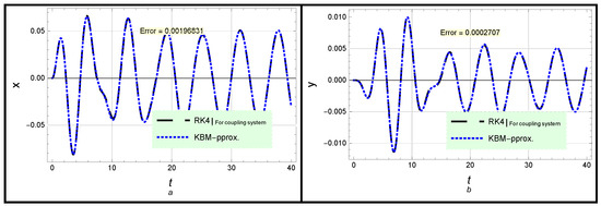
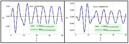
Now, we can apply two methodologies for analyzing the coupled system of FDDOs (41). In the first methodology, we can use the KBM analytical approximation (34) for studying the properties of the decoupled system oscillators (42) and then make a comparison among the obtained results and the RK4 approximations to the coupling system (41) as illustrated in Figure 1. In the second methodology, we can directly analyze the decoupling system of oscillators (42) using the RK4 approximations (here we do not use approximation (34)) and compare the numerical results with the RK4 approximations to the coupling system (41) as shown in Figure 2. Furthermore, the maximum residual distance error for the two methodologies is estimated as follows
It is noted from both Figure 1 and Figure 2 and the maximum error given in Equation (45) that both analytical and numerical approximations are compatible with each other, which confirms the high accuracy of the analytical solutions.
Example 2.
Let us now consider the following numerical example to the coupled system of FDDOs (6)
The decoupling system for system (46) reads
with
The KBM explicit form approximations to decoupled system (46) read
and
with
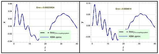
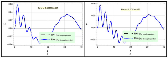
Both analytical approximations using the KBM method for the decoupling system (47) and the RK4 numerical approximation to coupled system (46) were compared with each other as shown in Figure 3. Moreover, the RK4 numerical approximations to the coupling system (46) and decoupling system (47) are introduced in Figure 4. Over and above, the maximum residual distance error for the two methodologies was estimated using the same parameters of Figure 3 as follows
It is evident that both analytical and numerical solutions exhibit a high degree of accuracy and stability for a long time.
4. Conclusions
The coupled forced damped Duffing oscillators (FDDOs) were analyzed analytically and numerically using highly accurate approximate methods. In our investigation, two different models for the coupled FDDOs were analyzed in detail. For the analytical approximation to the proposed models, the Krylov–Bogoliubov–Mitropolsky (KBM) method was used for solving the coupled FDDOs. However, to apply the mentioned method, the coupled FDDOs were reduced to a decoupled system of two individual standard FDDOs. After that, the proposed method was applied to find some approximations for both unforced and forced damped Duffing oscillators in terms of trigonometric functions. Some numerical examples using the KBM approximations were analyzed and discussed. Moreover, the KBM analytical approximations to the decoupled system and the RK4 numerical approximations to the coupled and decoupled systems were compared with each other to verify the high accuracy of all obtained approximations. Furthermore, the maximum residual error for all obtained approximations was estimated on the whole time domain. It was found that both analytical and numerical approximations were compatible with each other, which confirmed the high accuracy of the obtained approximations.
Author Contributions
Conceptualization, A.H.S. and S.A.E.-T.; methodology, A.H.S. and S.A.E.-T.; software, A.H.S. and S.A.E.-T.; validation, M.A.H., B.M.A. and L.S.E.-S.; formal analysis, A.H.S. and S.A.E.-T.; investigation, M.A.H., B.M.A. and L.S.E.-S.; resources, M.A.H., B.M.A. and L.S.E.-S.; data curation, M.A.H., B.M.A. and L.S.E.-S.; writing—original draft preparation, M.A.H., B.M.A. and L.S.E.-S.; writing—review and editing, A.H.S. and S.A.E.-T.; visualization, M.A.H., B.M.A. and L.S.E.-S.; supervision, A.H.S. and S.A.E.-T.; project administration, A.H.S. and S.A.E.-T. All authors have read and agreed to the published version of the manuscript.
Funding
The authors express their gratitude to Princess Nourah bint Abdulrahman University Researchers Supporting Project (grant no. PNURSP2022R32), Princess Nourah bint Abdulrahman University, Riyadh, Saudi Arabia.
Institutional Review Board Statement
Not applicable.
Informed Consent Statement
Not applicable.
Data Availability Statement
All data generated or analyzed during this study are included in this published article (More details can be requested from El-Tantawy).
Acknowledgments
The authors express their gratitude to Princess Nourah bint Abdulrahman University Researchers Supporting Project (Grant No. PNURSP2022R32), Princess Nourah bint Abdulrahman University, Riyadh, Saudi Arabia.
Conflicts of Interest
The authors declare that they have no conflict of interest.
Appendix A. The Coefficients of Equation (36)
Appendix B. The Values of the Coefficients Si of Equation (39)
References
- Tunç, C.; Tunç, O. A note on the stability and boundedness of solutions to non-linear differential systems of second order. J. Assoc. Arab Univ. Basic Appl. Sci. 2017, 24, 169. [Google Scholar] [CrossRef]
- Moulai-Khatir, A.; Remili, M.; Beldjerd, D. On asymptotic behaviors for a kind of third order neutral delay differential equations. An. Univ. Din Oradea Fasc. Mat. 2020, 27, 5–16. [Google Scholar]
- Duffing, G. Erzwungene schwingungen bei veränderlicher eigenfrequenz und ihre technische bedeutung. In Vieweg und Sohn, Braunschweig Sammlung Vieweg; Vieweg: Braunschweig, Germany, 1918; pp. 41–42. [Google Scholar]
- Hernández, J.M. The Duffing Oscillator Equation and Its Applications in Physics. Math. Probl. Eng. 2021, 2021, 9994967. [Google Scholar]
- Narasimha, R. Non-linear vibration of an elastic string. J. Sound Vib. 1968, 8, 134. [Google Scholar] [CrossRef]
- Sabarathinam, S.; Thamilmaran, K.; Borkowski, L.; Perlikowski, P.; Brzeski, P.; Stefanski, A.; Kapitaniak, T. Transient chaos in two coupled, dissipatively perturbed Hamiltonian Duffing oscillators. Commun. Nonlinear Sci. Numer. Simulat. 2013, 18, 3098. [Google Scholar] [CrossRef]
- Jothimurugan, R.; Thamilmaran, K.; Rajasekar, S.; Sanjuán, M.A.F. Multiple resonance and anti-resonance in coupled Duffing oscillators. Nonlinear Dyn. 2016, 83, 1803. [Google Scholar] [CrossRef]
- Musielak, D.E.; Musielak, Z.E.; Benner, J.W. Chaos and routes to chaos in coupled Duffing oscillators with multiple degrees of freedom. Chaos Solitons Fractals 2005, 24, 907. [Google Scholar] [CrossRef]
- Lenci, S. Exact solutions for coupled Duffing oscillators. Mech. Syst. Signal Process. 2022, 165, 108299. [Google Scholar] [CrossRef]
- Vincent, U.E.; Njah, A.N.; Akinlade, O.; Solarin, A.R.T. Synchronization of Cross-Well Chaos in Coupled Duffing Oscillators. Int. J. Mod. Phys. B 2005, 19, 3205. [Google Scholar] [CrossRef]
- Alhejaili, W.; Salas, A.H.; El-Tantawy, S.A. Approximate solution to a generalized Van der Pol equation arising in plasma oscillations. AIP Adv. 2022, 12, 105104. [Google Scholar] [CrossRef]
- Salas, A.H.; Albalawi, W.; El-Tantawy, S.A.; El-Sherif, L.S. Some Novel Approaches for Analyzing the Unforced and Forced Duffing–Van der Pol Oscillators. J. Math. 2022, 2022, 2174192. [Google Scholar] [CrossRef]
- Cai, J. A Generalized KBM Method for Strongly Nonlinear Oscillators with Slowly Varying Parameters. Math. Comput. Appl. 2007, 12, 21–30. [Google Scholar] [CrossRef]
- Alhejaili, W.; Salas, A.H.; El-Tantawy, S.A. Novel Approximations to the (Un)forced Pendulum–Cart System: Ansatz and KBM Methods. Mathematics 2022, 10, 2908. [Google Scholar] [CrossRef]
- Yamgoué, S.B.; Kofanxex, T.C. Application of the Krylov–Bogoliubov–Mitropolsky method to weakly damped strongly non-linear planar Hamiltonian systems. Int. J. Non-Linear Mech. 2007, 42, 1240. [Google Scholar] [CrossRef]
- Alyousef, H.A.; Salas, A.H.; Alharthi, M.R.; El-Tantawy, S.A. Galerkin method, ansatz method, and He’s frequency formulation for modeling the forced damped parametric driven pendulum oscillators. J. Low Freq. Noise Vib. Act. Control 2022, 41, 1426. [Google Scholar] [CrossRef]
- El-Dib, Y.O. The periodic property of Gaylord’s oscillator with a non-perturbative method. Arch. Appl. Mech. 2022, 92, 3067. [Google Scholar] [CrossRef]
- El-Dib, Y.O. An efficient approach to solving fractional Van der Pol–Duffing jerk oscillator. Commun. Theor. Phys. 2022, 74, 105006. [Google Scholar] [CrossRef]
- El-Dib, Y.O.; Elgazery, N.S. A novel pattern in a class of fractal models with the non-perturbative approach. Chaos Solitons Fractals 2022, 164, 112694. [Google Scholar] [CrossRef]
- Bezziou, M.; Jebril, I.; Dahmani, Z. A new nonlinear duffing system with sequential fractional derivatives. Chaos Solitons Fractals 2021, 151, 111247. [Google Scholar] [CrossRef]
- Hammad, M.A.; Salas, A.H.; El-Tantawy, S.A. New method for solving strong conservative odd parity nonlinear oscillators: Applications to plasma physics and rigid rotator. Aip Adv. 2020, 10, 085001. [Google Scholar] [CrossRef]
Publisher’s Note: MDPI stays neutral with regard to jurisdictional claims in published maps and institutional affiliations. |
© 2022 by the authors. Licensee MDPI, Basel, Switzerland. This article is an open access article distributed under the terms and conditions of the Creative Commons Attribution (CC BY) license (https://creativecommons.org/licenses/by/4.0/).