Fractional Stefan Problem Solving by the Alternating Phase Truncation Method

Abstract

The aim of this paper is the adaptation of the alternating phase truncation (APT) method for solving the two-phase time-fractional Stefan problem. The aim was to determine the approximate temperature distribution in the domain with the moving boundary between the solid and the liquid phase. The adaptation of the APT method is a kind of method that allows us to consider the enthalpy distribution instead of the temperature distribution in the domain. The method consists of reducing the whole considered domain to liquid phase by adding sufficient heat at each point of the solid and then, after solving the heat equation transformed to the enthalpy form in the obtained region, subtracting the heat that has been added. Next the whole domain is reduced to the solid phase by subtracting the sufficient heat from each point of the liquid. The heat equation is solved in the obtained region and, after that, the heat that had been subtracted is added at the proper points. The steps of the APT method were adapted to solve the equations with the fractional derivatives. The paper includes numerical examples illustrating the application of the described method.

1. Introduction

In the 20th century, fractional calculus began to be used to model the various processes. Among various applications of fractional calculus, a high position is occupied by the heat conduction problems. Models containing the fractional derivatives can rarely be solved in an exact way. Hence, the numerical methods of solving such problems gained great popularity. In the paper [1] the authors show that the fractional derivatives can be used to model the anomalous diffusion phenomenon that occurs in the ceramic materials, composites and porous materials. In the paper [2], the authors consider the model of the heat conduction process in ceramic material using the fractional derivative of Grünwald-Letnikov type, and on the basis of the experimental verification, they show that this model gives better results than the model with the classic derivative. In the papers [3,4] the authors deal with the heat conduction problem in porous aluminum using various models with the classic derivative, the fractional derivative of Caputo type and the fractional derivative of Riemann–Liouville type, and then they perform the experimental verification of the obtained results. A model with the fractional derivative of Caputo type was applied in the paper [5] to describe the heat conduction process in the composite material. Fractional calculus was also used for the other heat conduction processes, such as the study of the diffusion process in brick [6], modeling of the growth of frost on a flat plate [7] and study of the anomalous diffusion of drug release from a slab matrix [8].

In the last decades, to analyze and solve the models containing fractional derivatives, the following methods were applied: the finite difference method [9,10,11], the finite element method [12], the local discontinuous Galerkin method [13], and the spline collocation method [14].

Recently, research has been carried out on the fractional Stefan problem. The Stefan problem consists of finding the temperature distribution in the system in which the phase transition takes place, and the position of the moving boundary separating the phases changes. It owes its name to the physicist Jozef Stefan [15], who was one of the first researchers investigating the processes with phase transitions. This problem was previously investigated by Lamé and Clapeyron in the paper [16]. Stefan investigated the process of ice sheet formation based on the measurements collected by English and German polar expeditions [17]. Stefan’s model, presented in the paper [18] in 1889, was the first to account for the energy conservation condition at the boundary separating the phases, which was later named after him. In the paper [19], to solve the Stefan problem, the authors applied the alternating phase truncation method. A classic Stefan problem is described in more detail in the books [20,21].

The one-dimensional one-phase time- and space-fractional Stefan problem has recently been widely studied. In the paper [22] Voller presents various models of the Stefan problem with the fractional derivatives of Caputo and Riemann–Liouville type. The review of various time-fractional Stefan problem models is also presented in the paper [23]. A physical interpretation of such problems is described in the paper [24]. Kubica and Ryszewska [25] present the analysis of a self-similar solution of this problem. Ryszewska, in turn, in paper [26] proves the existence and explicitness of solution of the one-phase one-dimensional space-fractional Stefan problem, whereas Athanasopoulos et al. [27] prove that the weak solution of the two-phase space-fractional Stefan problem is continuous. The problem is formulated via the singular nonlinear parabolic integro-differential equations.

The Stefan problem with the fractional derivative has an analytical solution only for the simple one-phase case or in the semi-infinite region [28,29,30,31,32,33]. In paper [32], Roscani and Tarzia present the explicit solution of a one-phase time-fractional Stefan problem in terms of the Wright functions. Roscani et al. [31] present self-similar solutions for the one-phase one-dimensional space-fractional Stefan problem in terms of the Mittag–Leffler function. The analytical solutions of the two-phase problem in a semi-infinite domain are presented in papers [29,33]. The solutions are given through the Wright and Mainardi functions.

The papers concerning the numerical methods of solving the fractional Stefan problem are still sparse. Błasik and Klimek [34] use the front-fixing method to solve the one-dimensional one-phase time-fractional Stefan problem. In paper [35], the similarity variable and the finite difference methods were used to solve the same problem. Rajeev and Kushwaha [36] use the homotopy perturbation method to solve the one-dimensional one-phase time-fractional Stefan problem. To solve the one-phase space-fractional Stefan problem, Gao et al. [37] use the boundary immobilization technique based on the explicit finite difference. Garshasbi and Sanaei [38] apply the iterative implicit finite difference method to solve the one-phase one-dimensional space-fractional Stefan problem. An explicit finite difference method scheme for solving the same kind of problem was used in the paper [39].

The method of solving the two-phase one-dimensional problem is presented by Blłasik in the paper [40]. In the proposed algorithm, Błasik uses a special case of the front-fixing method supplemented by the iterative procedure. In the paper [41], Rajeev obtains the approximate solution of the fractional Stefan problem by using the homotopy analysis method. In the homotopy analysis method the solution is obtained as a series which often has a small convergence region.

The fractional Stefan problem can be applied for modeling different phenomena, such as the drug release from the polymer matrix [8,38,42], the sediment transport problem [36,43], and the heat conduction in the porous materials [44,45].

Motivation for adapting the alternating phase truncation method to solve the time-fractional Stefan problem was given, on one hand, by a sparse number of papers concerning the solution of two-phase problem and, on the other hand, by the limitations of available methods. Due to their constructions, both of the above mentioned methods are of little use in the algorithms for solving the inverse problems, where the direct problem must be solved repeatedly. In the future, the presented method is planned to be applied to solve the inverse fractional Stefan problem.

In this article, we will consider the one-dimensional two-phase time-fractional Stefan problem. The temperature derivative with respect to time will be a fractional derivative of Caputo type. The problem will be solved with application of the alternating phase truncation method adapted to the equations with the fractional derivatives. A shortened version of this paper was presented at the conference [46]. In the problems of heat flow, we often deal with the thermal symmetry. This allows us to consider only a part of the area and transfer the obtained results symmetrically to the rest of the area. Additionally, the issue considered in this paper can be treated as a part of larger whole resulting from thermal symmetry.

The paper is organized as follows. In Section 2, the formulation of the problem is presented. Section 3 is devoted to the description of the method of the solution. In Section 4, the discretization of the region and equations is described. Section 5, in turn, contains the description of APT algorithm. To illustrate the application of the described method, two numerical examples are presented in Section 6 and Section 7. The last section includes the conclusions.

2. Formulation of the Problem

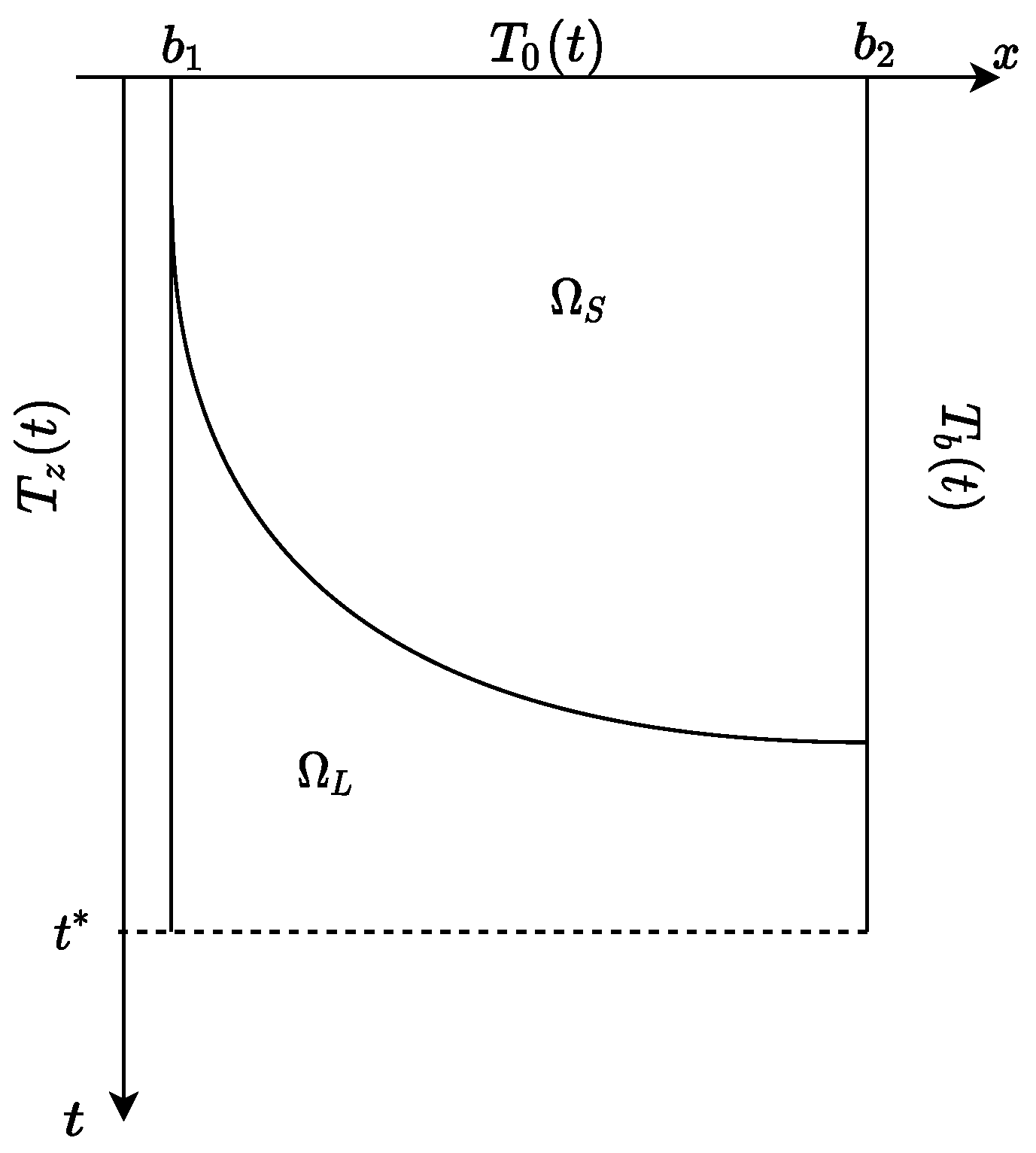
We consider the one-dimensional two-phase Stefan problem. The considered area is divided into two sub-areas: ${\mathrm{\Omega }}_S$ occupied by the solid phase and ${\mathrm{\Omega }}_L$ occupied by the liquid phase (see Figure 1). The moving boundary separating the phases is described by the function $x=s\left(t\right)$.

In the model, the fractional derivative of Caputo type of order $\alpha$ is used, which for $\alpha \in (n-1,n)$, $n\in \mathbb{N}$, is defined by the formula [47,48]

$$D_x^{\alpha }f\left(x\right)=\frac{1}{\mathrm{\Gamma }(n-\alpha )}{\int }_0^x{(x-\tau )}^{n-\alpha -1}{f}^{\left(n\right)}\left(\tau \right)d\tau ,$$

where $\mathrm{\Gamma }$ is the gamma function defined on the set ${\mathbb{R}}_{+}$ as

$$\mathrm{\Gamma }\left(x\right)={\int }_0^{\infty }{t}^{x-1}{e}^{-t}dt.$$

We consider the one-dimensional case of the two-phase fractional Stefan problem for the melting process for $x\in [b_1,b_2]$. In the considered area, there are two separate subareas of the solid and liquid phase. The direct Stefan problem consists of finding the temperature distribution $T_S$ and $T_L$ in the proper sub-area and the position of the boundary separating the phases for the given set of initial boundary conditions and values of thermophysical parameters. The temperature distribution in both subareas is a solution of the heat conduction equation where the derivative with respect to time is the derivative of fractional order $\alpha$ of Caputo type, and the derivative with respect to space is the classical derivative

$$\begin{array}{cc}\hfill c_L{\rho }_L{D}_t^{\alpha }{T}_L(x,t)& ={\overline{\lambda }}_L\frac{{\partial }^2{T}_L(x,t)}{\partial x^2},b_1<x<s\left(t\right),t\in (0,t^{*}),\hfill \end{array}$$

(1)

$$\begin{array}{cc}\hfill c_S{\rho }_S{D}_t^{\alpha }{T}_S(x,t)& ={\overline{\lambda }}_S\frac{{\partial }^2{T}_S(x,t)}{\partial x^2},s\left(t\right)<x<b_2,t\in (0,t^{*}),\hfill \end{array}$$

(2)

where $c_k$—specific heat [$\mathrm{J}/\left(\mathrm{kg}\mathrm{K}\right)$], ${\rho }_k$—density [$\mathrm{kg}/{\mathrm{m}}^3$], ${\overline{\lambda }}_k=\overline{w}{\lambda }_k$—the scaled thermal conductivity [$\mathrm{W}/\left({\mathrm{s}}^{\alpha -1}\mathrm{m}\mathrm{K}\right)$], that is the thermal conductivity multiplied by the scaling constant $\overline{w}$ with numerical value of one and unit [${\mathrm{s}}^{1-\alpha }$] chosen such that the right and left units of the equation are the same [4,49,50], ${\lambda }_k$–thermal conductivity [$\mathrm{W}/\left(\mathrm{m}\mathrm{K}\right)$], where index $k=S$ denotes the solid phase and $k=L$ the liquid phase. We assume that the values of the parameters $c_S$, ${\rho }_S$, ${\overline{\lambda }}_S$, $c_L$, ${\rho }_L$, ${\overline{\lambda }}_L$ are constant.

At the moment $t=0$, the initial condition in the considered region is as follows

$$T_S(x,0)=T_0\left(x\right),b_1\le x\le b_2.$$

(3)

For $t>0$ at the point $x=b_1$ we set the boundary condition of the first kind

$$T_k(b_1,t)=T_z\left(t\right),t\in (0,t^{*}),k\in \{L,S\},$$

(4)

and at the point $x=b_2$, we also define the boundary condition of the first kind

$$T_k(b_2,t)=T_b\left(t\right),t\in (0,t^{*}),k\in \{L,S\}.$$

(5)

On the moving boundary s, that separates the two phases, the condition of the temperature continuity and the Stefan condition are set. The Stefan condition with the fractional derivative of Caputo type with respect to time is the following

$${\displaystyle -{\overline{\lambda }}_L{\left.\frac{\partial T_L(x,t)}{\partial x}\right|}_{x=s\left(t\right)}=-{\overline{\lambda }}_S{\left.\frac{\partial T_S(x,t)}{\partial x}\right|}_{x=s\left(t\right)}+L{\rho }_S{D}_t^{\alpha }s\left(t\right),}$$

(6)

where L is the latent heat of fusion by unit of mass [$\mathrm{J}/\mathrm{kg}$]. The temperature continuity condition is expressed by the formula

$$T_S(s\left(t\right),t)=T_L(s\left(t\right),t)=T_m,$$

(7)

where $T_m$ [$\mathrm{K}$] denotes the temperature of the phase transition.

3. Method of Solution

The alternating phase truncation method was described for the first time in the paper [51] by Rogers, Berger and Ciment. It belongs to the group of methods in which the problem is formulated in such a way that the Stefan condition does not appear in the model in the explicit form. In the paper [19], this method was used by the same authors to solve the two-phase Stefan problem. In the alternating phase truncation method the enthalpy, expressed by the unit of volume, is considered instead of the temperature.

The enthalpy, expressed by the unit of volume, is described by the formula [52]:

$$H\left(T\right)={\int }_0^{T}c\left(\mu \right)\rho \left(\mu \right)d\mu +\eta \left(T\right)L{\rho }_S,$$

(8)

where $\eta$ is a function defined as

$$\eta \left(T\right)=\left\{\begin{array}{cc}0\hfill & \mathrm{for}T\le T_m,\hfill \\ 1\hfill & \mathrm{for}T>T_m.\hfill \end{array}\right.$$

This function has the discontinuity point at point $T_m$. The one-sided enthalpy limits of (8) at this point are the following

$$\begin{array}{cc}\hfill A_1& =\underset{T\to T_m^{-}}{lim}H\left(T\right)={\int }_0^{T_m}c\left(\mu \right)\rho \left(\mu \right)d\mu ,\hfill \end{array}$$

(9)

$$\begin{array}{cc}\hfill A_2& =\underset{T\to T_m^{+}}{lim}H\left(T\right)={\int }_0^{T_m}c\left(\mu \right)\rho \left(\mu \right)d\mu +L{\rho }_S.\hfill \end{array}$$

(10)

Introducing the notation $\kappa =L{\rho }_S$, where $\kappa$ [$\mathrm{J}/{\mathrm{m}}^3$] denotes the latent heat of fusion by the unit of volume, the limit

$$A_2=A_1+\kappa .$$

(11)

For the constant $c_S,c_L,{\rho }_S,{\rho }_L$ function (8) takes the form

$$H\left(T\right)=\left\{\begin{array}{cc}{c}_S{\rho }_{S}T\hfill & \mathrm{for}T\le T_m,\hfill \\ c_L{\rho }_L(T-T_m)+c_S{\rho }_S{T}_m+\kappa \hfill & \mathrm{for}T>T_m.\hfill \end{array}\right.$$

(12)

Function $T\left(H\right)$ is obtained as the inverse function of function (12). Hence, the function $T\left(H\right)$ takes the form

$$T\left(H\right)=\left\{\begin{array}{cc}\frac{1}{c_S{\rho }_S}H\hfill & \mathrm{for}T\le T_m\Rightarrow H\le A_1,\hfill \\ T_m\hfill & \mathrm{for}H\in (A_1,A_2],\hfill \\ T_m+\frac{1}{c_L{\rho }_L}(H-c_S{\rho }_S{T}_m-\kappa )\hfill & \mathrm{for}T>T_m\Rightarrow H>A_2.\hfill \end{array}\right.$$

Now, let the derivative of the enthalpy with respect to time be the fractional derivative of the Caputo type of order $\alpha \in (0,1)$, and the derivative with respect to space be the classic derivative. We calculate the fractional derivative of enthalpy of the Caputo type of order $\alpha$:

$$\begin{array}{cc}\hfill & D_t^{\alpha }{H}_k(x,t)=\frac{1}{\mathrm{\Gamma }(1-\alpha )}{\int }_0^t{(t-\tau )}^{-\alpha }{\left.\frac{\partial H_k}{\partial t}\right|}_{t=\tau }d\tau \hfill \\ \hfill & =\frac{1}{\mathrm{\Gamma }(1-\alpha )}{\int }_0^t{(t-\tau )}^{-\alpha }{c}_k{\rho }_k{\left.\frac{\partial T_k}{\partial t}\right|}_{t=\tau }d\tau =c_k{\rho }_k{D}_t^{\alpha }{T}_k(x,t)\hfill \\ \hfill & =\frac{1}{\mathrm{\Gamma }(1-\alpha )}{\int }_0^{t_x}{(t-\tau )}^{-\alpha }{c}_S{\rho }_S{\left.\frac{\partial T_S}{\partial t}\right|}_{t=\tau }d\tau +\frac{1}{\mathrm{\Gamma }(1-\alpha )}{\int }_{t_x}^t{(t-\tau )}^{-\alpha }{c}_L{\rho }_L{\left.\frac{\partial T_L}{\partial t}\right|}_{t=\tau }d\tau \hfill \\ \hfill & =c_S{\rho }_S{D}_t^{\alpha }{T}_S(x,t_x)+c_L{\rho }_L(D_t^{\alpha }{T}_L(x,t)-D_t^{\alpha }{T}_S(x,t_x))\hfill \\ \hfill & =(c_S{\rho }_S-c_L{\rho }_L)D_t^{\alpha }{T}_S(x,t_x)+c_L{\rho }_L{D}_t^{\alpha }{T}_L(x,t),\hfill \end{array}$$

(13)

where $t_x$ is the moment of time when the phase transition from the solid to liquid phase happens at point x.

Function (13) can be formulated as

$$D_t^{\alpha }{H}_k(x,t)=\left\{\begin{array}{cc}{c}_S{\rho }_S{D}_t^{\alpha }{T}_S(x,t)\hfill & \mathrm{for}t\le t_x,\hfill \\ (c_S{\rho }_S-c_L{\rho }_L)D_t^{\alpha }{T}_S(x,t_x)+c_L{\rho }_L{D}_t^{\alpha }{T}_L(x,t)\hfill & \mathrm{for}t>t_x,\hfill \end{array}\right.$$

(14)

By transforming (14), we obtain the Caputo derivative of order $\alpha$ of the temperature function

$$D_t^{\alpha }{T}_k(x,t)=\left\{\begin{array}{cc}\frac{1}{c_S{\rho }_S}{D}_t^{\alpha }{H}_S(x,t)\hfill & \mathrm{for}t\le t_x,\hfill \\ \frac{1}{c_L{\rho }_L}{D}_t^{\alpha }{H}_L(x,t)-\left(\frac{c_S{\rho }_S}{c_L{\rho }_L}-1\right)D_t^{\alpha }{T}_S(x,t_x)\hfill & \mathrm{for}t>t_x,\hfill \end{array}\right.$$

(15)

After introducing the function

$$G(x,t)=\left\{\begin{array}{cc}0\hfill & \mathrm{for}t\le t_x,\hfill \\ \left(\frac{c_S{\rho }_S}{c_L{\rho }_L}-1\right)D_t^{\alpha }{T}_S(x,t_x)\hfill & \mathrm{for}t>t_x,\hfill \end{array}\right.$$

the temperature derivative (15) can be formulated as

$$D_t^{\alpha }{T}_k(x,t)=\frac{1}{c_k{\rho }_k}{D}_t^{\alpha }{H}_k(x,t)-G(x,t).$$

(16)

By differentiating the enthalpy with respect to the space variable, we obtain

$$\frac{\partial H_k(x,t)}{\partial x}=\frac{d{H}_k\left(T\right)}{d{T}_k}\frac{\partial T_k(x,t)}{\partial x}=c_k{\rho }_k\frac{\partial T_k(x,t)}{\partial x}.$$

The second derivative of enthalpy with respect to the space variable is as follows

$$\frac{{\partial }^2{H}_k(x,t)}{\partial x^2}=\frac{\partial }{\partial x}\frac{\partial H_k(x,t)}{\partial x}=\frac{\partial }{\partial x}\left(c_k{\rho }_k\frac{\partial T_k(x,t)}{\partial x}\right)=c_k{\rho }_k\frac{{\partial }^2{T}_k(x,t)}{\partial x^2}.$$

(17)

By transforming (17), we obtain

$$\frac{{\partial }^2{T}_k(x,t)}{\partial x^2}=\frac{1}{c_k{\rho }_k}\frac{{\partial }^2{H}_k(x,t)}{\partial x^2}.$$

(18)

Using (16) and (18) the equation of the heat conduction can be written as

$$D_t^{\alpha }{H}_k(x,t)-c_k{\rho }_{k}G(x,t)={\overline{a}}_k\frac{{\partial }^2{H}_k(x,t)}{\partial x^2}.$$

(19)

where ${\overline{a}}_k=\frac{{\overline{\lambda }}_k}{c_k{\rho }_k}$ [$m^2/s^{\alpha }$]. By introducing the additional designation $G_1(x,t)=c_k{\rho }_{k}G(x,t)$, we can reduce the Equation (19) to the form

$$D_t^{\alpha }{H}_k(x,t)={\overline{a}}_k\frac{{\partial }^2{H}_k(x,t)}{\partial x^2}+G_1(x,t).$$

(20)

The Stefan condition (6) with the fractional derivative of Caputo type in the enthalpy convention takes the form

$$-{\overline{a}}_L{\left.\frac{\partial H_L(x,t)}{\partial x}\right|}_{x=s\left(t\right)}=-{\overline{a}}_S{\left.\frac{\partial H_S(x,t)}{\partial x}\right|}_{x=s\left(t\right)}+\kappa D_t^{\alpha }s\left(t\right),$$

and instead of the temperature continuity condition (7) we receive the condition

$$A_2=A_1+\kappa .$$

The considered model of the Stefan problem (1)–(7) in the enthalpy convention for $t\in (0,t^{*})$ takes the form

$$\begin{array}{cc}\hfill & D_t^{\alpha }{H}_L(x,t)={\overline{a}}_L\frac{{\partial }^2{H}_L(x,t)}{\partial x^2},b_1<x<s\left(t\right),\hfill \\ \hfill & D_t^{\alpha }{H}_S(x,t)={\overline{a}}_S\frac{{\partial }^2{H}_S(x,t)}{\partial x^2},s\left(t\right)<x<b_2,\hfill \\ \hfill & -{\overline{a}}_L{\left.\frac{\partial H_L(x,t)}{\partial x}\right|}_{x=s\left(t\right)}=-{\overline{a}}_S{\left.\frac{\partial H_S(x,t)}{\partial x}\right|}_{x=s\left(t\right)}+\kappa D_t^{\alpha }s\left(t\right),\hfill \\ \hfill & A_2=A_1+\kappa ,\hfill \\ \hfill & H_S(x,0)=H\left(T_0\left(x\right)\right),b_1\le x\le b_2,\hfill \\ \hfill & {\left.H_k(x,t)\right|}_{x=b_1}=H\left(T_z\left(t\right)\right),k\in \{L,S\},\hfill \\ \hfill & {\left.H_k(x,t)\right|}_{x=b_2}=H\left(T_b\left(t\right)\right),k\in \{L,S\}.\hfill \end{array}$$

(21)

In the APT method, each time step is divided into two stages. In the first stage, we reduce the entire considered area to the liquid phase by adding a certain amount of heat at the points occupied by the solid phase. Then, we solve the heat conduction problem in the liquid phase and the obtained enthalpy distribution, after subtracting the proper amount of heat at the points where it was previously added, becomes the starting point for the next stage. In the second stage, the entire area is reduced to the solid phase by subtracting a certain amount of heat at the points occupied by the liquid phase. Next, we solve the heat conduction problem in the solid phase. The obtained enthalpy distribution, after adding the proper amount of heat at the points where it was previously subtracted, completes one step of the calculations.

In the alternating phase truncation method for each time step, the heat conduction equation is solved twice. Hence, it must be taken into account that the boundary conditions must affect the considered system only for the time $\Delta t$, and not for the $2\Delta t$. In the first step of the method, the boundary conditions are taken into account on these pieces of the boundary where the contact between the liquid phase and the surroundings takes place. The remaining pieces of boundary are isolated; that is, the following condition is made

$$-{\overline{a}}_k\frac{\partial H_k(x,t)}{\partial x}=0.$$

In the second step, the real boundary conditions are taken into account on these pieces of the boundary where the contact of the solid phase and the surrounding takes place, and the remaining pieces of the boundary are isolated.

4. Discretization

In the domain of space, we introduce the grid: $x_i=i\Delta x$, $i=0,1,\dots ,N$ and in the domain of time, the grid: $t_j=j\Delta t$, $j=0,1,\dots ,K$. For simplicity, from now on we will omit the index $k\in \{S,L\}$. Belonging to the proper phase will be identified basing on the value of the enthalpy (temperature) in the given point. Hence, we introduce the notation $H(x_i,t_j)=H_i^j$.

We approximate the Caputo derivative, where $\alpha \in (0,1),$ in the following way [9,10,53]:

$$\begin{array}{cc}\hfill & D_t^{\alpha }{H}_i^j=\frac{1}{\mathrm{\Gamma }(1-\alpha )}{\int }_0^{t_j}{(t_j-s)}^{-\alpha }\frac{\partial H(x_i,s)}{\partial t}ds\hfill \\ \hfill & =\frac{1}{\mathrm{\Gamma }(1-\alpha )}\sum _{r=1}^j{\int }_{t_{r-1}}^{t_r}{(t_j-s)}^{-\alpha }\left(\frac{H_i^r-H_i^{r-1}}{\Delta t}\right)ds\hfill \\ \hfill & =\frac{1}{\mathrm{\Gamma }(1-\alpha )}\sum _{r=1}^j{\int }_{(r-1)\Delta t}^{r\Delta t}{(j\Delta t-s)}^{-\alpha }\left(\frac{H_i^r-H_i^{r-1}}{\Delta t}\right)ds\hfill \\ \hfill & =\frac{1}{\mathrm{\Gamma }(1-\alpha )}\frac{1}{1-\alpha }\sum _{r=1}^j\left[\left({(j-r+1)}^{1-\alpha }-{(j-r)}^{1-\alpha }\right)\frac{H_i^r-H_i^{r-1}}{\Delta t}\right]{(\Delta t)}^{1-\alpha }\hfill \\ \hfill & =\frac{1}{\mathrm{\Gamma }(1-\alpha )}\frac{1}{1-\alpha }\frac{1}{{(\Delta t)}^{\alpha }}\sum _{r=1}^j\left(H_i^r-H_i^{r-1}\right)\left({(j-r+1)}^{1-\alpha }-{(j-r)}^{1-\alpha }\right)\hfill \\ \hfill & =\frac{1}{\mathrm{\Gamma }(1-\alpha )}\frac{1}{1-\alpha }\frac{1}{{(\Delta t)}^{\alpha }}\sum _{r=1}^j\left(r^{1-\alpha }-{(r-1)}^{1-\alpha }\right)\left(H_i^{j-r+1}-H_i^{j-r}\right).\hfill \end{array}$$

(22)

We introduce the following notation

$$\sigma (\alpha ,\Delta t)=\frac{1}{\mathrm{\Gamma }(1-\alpha )(1-\alpha ){(\Delta t)}^{\alpha }},$$

$$\omega (\alpha ,r)=r^{1-\alpha }-{(r-1)}^{1-\alpha }.$$

By applying the above notation to the approximated derivative (22), we finally get

$$D_t^{\alpha }{H}_i^j=\sigma (\alpha ,\Delta t)\sum _{r=1}^j\omega (\alpha ,r)\left(H_i^{j-r+1}-H_i^{j-r}\right).$$

(23)

The second-order derivative of enthalpy with respect to the space variable is approximated by using the second-order differential quotient

$${\left.\frac{{\partial }^{2}H}{\partial x^2}\right|}_{(x_i,t_j)}=\frac{H_{i+1}^j-2H_i^j+H_{i-1}^j}{{(\Delta x)}^2}.$$

(24)

Using (23) and (24), we can formulate the equation of the heat conduction (20) in the discrete form

$$\sigma (\alpha ,\Delta t)\sum _{r=1}^j\omega (\alpha ,r)\left(H_i^{j-r+1}-H_i^{j-r}\right)=\overline{a}\frac{H_{i+1}^j-2H_i^j+H_{i-1}^j}{{(\Delta x)}^2}+G_{1,i}^j.$$

(25)

By transforming the obtained Equation (25) we reduce it to the form

$$\begin{array}{cc}\hfill & \sigma (\alpha ,\Delta t)\left[\omega (\alpha ,1)\left(H_i^j-H_i^{j-1}\right)+\sum _{r=2}^j\omega (\alpha ,r)\left(H_i^{j-r+1}-H_i^{j-r}\right)\right]\hfill \\ \hfill & =\frac{\overline{a}}{{(\Delta x)}^2}\left(H_{i+1}^j-2H_i^j+H_{i-1}^j\right)+G_{1,i}^j,\hfill \end{array}$$

and after proper ordering, we get

$$\begin{array}{cc}\hfill & \sigma (\alpha ,\Delta t)\omega (\alpha ,1)H_i^j-\frac{\overline{a}}{{(\Delta x)}^2}{H}_{i-1}^j+\frac{2\overline{a}}{{(\Delta x)}^2}{H}_i^j-\frac{\overline{a}}{{(\Delta x)}^2}{H}_{i+1}^j\hfill \\ \hfill & =\sigma (\alpha ,\Delta t)\omega (\alpha ,1)H_i^{j-1}-\sigma (\alpha ,\Delta t)\sum _{r=2}^j\omega (\alpha ,r)\left(H_i^{j-r+1}-H_i^{j-r}\right)+G_{1,i}^j.\hfill \end{array}$$

(26)

It is known that $\omega (\alpha ,1)=1$, so the Equation (26) can be presented as

$$\begin{array}{cc}\hfill & -\frac{\overline{a}}{{(\Delta x)}^2}{H}_{i-1}^j+\left(\sigma (\alpha ,\Delta t)+\frac{2\overline{a}}{{(\Delta x)}^2}\right)H_i^j-\frac{\overline{a}}{{(\Delta x)}^2}{H}_{i+1}^j\hfill \\ \hfill & =\sigma (\alpha ,\Delta t)H_i^{j-1}-\sigma (\alpha ,\Delta t)\sum _{r=2}^j\omega (\alpha ,r)\left(H_i^{j-r+1}-H_i^{j-r}\right)+G_{1,i}^j.\hfill \end{array}$$

(27)

This is the heat conduction equation for the internal nodes $i=1,2,\dots ,N-1$.

We also need to find the difference equation for the boundary condition of the second kind, which appears while solving the heat conduction equation two times in each time step (see note at the end of the previous chapter).

The first-order derivative of enthalpy with respect to the space variable is approximated by using the central differential quotient

$${\left.\frac{\partial H}{\partial x}\right|}_{(x_i,t_j)}=\frac{H_{i+1}^j-H_{i-1}^j}{2\Delta x}.$$

Hence, for the node $x_0$, we obtain

$${\left.\frac{\partial H}{\partial x}\right|}_{(x_0,t_j)}=\frac{H_1^j-H_{-1}^j}{2\Delta x}.$$

(28)

Putting (28) into the boundary condition of the second kind, we obtain

$$-\overline{a}\frac{H_1^j-H_{-1}^j}{2\Delta x}=q^j.$$

(29)

By transforming (29), we receive

$$H_{-1}^j=H_1^j+\frac{2\Delta x}{\overline{a}}{q}^j.$$

(30)

The Equation (27) for $i=0$ has the form

$$\begin{array}{cc}\hfill & -\frac{\overline{a}}{{(\Delta x)}^2}{H}_{-1}^j+\left(\sigma (\alpha ,\Delta t)+\frac{2\overline{a}}{{(\Delta x)}^2}\right)H_0^j-\frac{\overline{a}}{{(\Delta x)}^2}{H}_1^j\hfill \\ \hfill & =\sigma (\alpha ,\Delta t)H_0^{j-1}-\sigma (\alpha ,\Delta t)\sum _{r=2}^j\omega (\alpha ,r)\left(H_0^{j-r+1}-H_0^{j-r}\right)+G_{1,0}^j.\hfill \end{array}$$

(31)

As a result of taking into account the Formula (30), the Equation (31) takes the form

$$\begin{array}{cc}\hfill & -\frac{\overline{a}}{{(\Delta x)}^2}{H}_1^j-\frac{2}{\Delta x}{q}^j+\left(\sigma (\alpha ,\Delta t)+\frac{2\overline{a}}{{(\Delta x)}^2}\right)H_0^j-\frac{\overline{a}}{{(\Delta x)}^2}{H}_1^j\hfill \\ \hfill & =\sigma (\alpha ,\Delta t)H_0^{j-1}-\sigma (\alpha ,\Delta t)\sum _{r=2}^j\omega (\alpha ,r)\left(H_0^{j-r+1}-H_0^{j-r}\right)+G_{1,0}^j,\hfill \end{array}$$

and after proper ordering, we obtain the energy equation, including the boundary condition of the second kind. Thus, for the point $x_0$, we obtain

$$\begin{array}{cc}\hfill & \left(\sigma (\alpha ,\Delta t)+\frac{2\overline{a}}{{(\Delta x)}^2}\right)H_0^j-\frac{2\overline{a}}{{(\Delta x)}^2}{H}_1^j\hfill \\ \hfill & =\frac{2}{\Delta x}{q}^j+\sigma (\alpha ,\Delta t)H_0^{j-1}-\sigma (\alpha ,\Delta t)\sum _{r=2}^j\omega (\alpha ,r)\left(H_0^{j-r+1}-H_0^{j-r}\right)+G_{1,0}^j.\hfill \end{array}$$

(32)

For the node $x_N$, the Equation (4) takes the form

$${\left.\frac{\partial H}{\partial x}\right|}_{(x_N,t_j)}=\frac{H_{N+1}^j-H_{N-1}^j}{2\Delta x}.$$

By applying it to the boundary condition of the second kind, we obtain

$$-\overline{a}\frac{H_{N+1}^j-H_{N-1}^j}{2\Delta x}={\overline{q}}^j.$$

(33)

By transforming (33), we receive

$$H_{N+1}^j=H_{N-1}^j-\frac{2\Delta x}{\overline{a}}{\overline{q}}^j.$$

(34)

The Equation (27) for $i=N$ takes the form

$$\begin{array}{cc}\hfill & -\frac{\overline{a}}{{(\Delta x)}^2}{H}_{N-1}^j+\left(\sigma (\alpha ,\Delta t)+\frac{2\overline{a}}{{(\Delta x)}^2}\right)H_N^j-\frac{\overline{a}}{{(\Delta x)}^2}{H}_{N+1}^j\hfill \\ \hfill & =\sigma (\alpha ,\Delta t)H_N^{j-1}-\sigma (\alpha ,\Delta t)\sum _{r=2}^j\omega (\alpha ,r)\left(H_N^{j-r+1}-H_N^{j-r}\right)+G_{1,N}^j.\hfill \end{array}$$

(35)

Let us apply formula (34), resulting from the boundary condition of the second kind, to the Equation (35). We get

$$\begin{array}{cc}\hfill & -\frac{\overline{a}}{{(\Delta x)}^2}{H}_{N-1}^j+\left(\sigma (\alpha ,\Delta t)+\frac{2\overline{a}}{{(\Delta x)}^2}\right)H_N^j-\frac{\overline{a}}{{(\Delta x)}^2}{H}_{N-1}^j+\frac{2}{\Delta x}{\overline{q}}^j\hfill \\ \hfill & =\sigma (\alpha ,\Delta t)H_N^{j-1}-\sigma (\alpha ,\Delta t)\sum _{r=2}^j\omega (\alpha ,r)\left(H_N^{j-r+1}-H_N^{j-r}\right)+G_{1,N}^j,\hfill \end{array}$$

hence, the final form of the equation, taking into account the boundary condition of the second kind, takes the form

$$\begin{array}{cc}\hfill & -\frac{2\overline{a}}{{(\Delta x)}^2}{H}_{N-1}^j+\left(\sigma (\alpha ,\Delta t)+\frac{2\overline{a}}{{(\Delta x)}^2}\right)H_N^j-\frac{\overline{a}}{{(\Delta x)}^2}{H}_{N-1}^j\hfill \\ \hfill & =-\frac{2}{\Delta x}{\overline{q}}^j+\sigma (\alpha ,\Delta t)H_N^{j-1}-\sigma (\alpha ,\Delta t)\sum _{r=2}^j\omega (\alpha ,r)\left(H_N^{j-r+1}-H_N^{j-r}\right)+G_{1,N}^j.\hfill \end{array}$$

(36)

To approximate the fractional derivative of Caputo type, we used the $L1$ method. The error of this method is of order $O(\Delta t^{2-\alpha })$ [9,10,53]. The second derivative with respect to space was approximated by applying the central difference quotient, for which the error is of the order $O(\Delta x^2)$ [54]. Therefore, the error of the scheme is of order $O(\Delta t^{2-\alpha }+\Delta x^2)$. Due to application of the implicit scheme, it is unconditionally stable. One can refer to [9,10,53,54] for more details.

5. APT Method Algorithm

To determine the temperature distribution in the considered area described by the model (21) the alternating phase truncation method is used. The method is adapted to the equations with the fractional derivatives of Caputo type.

In the alternating phase truncation method, each time step is divided into two stages. In the first stage, the entire considered area is conventionally reduced to the liquid phase, and the heat conduction equation is solved for it. The obtained enthalpy distribution, after subtracting the proper amount of heat at the points at which it was conventionally added earlier, becomes the starting point for the next stage. In the second stage, the entire considered area is conventionally reduced to the solid phase, and the heat conduction equation is also solved for it. The obtained enthalpy distribution, after adding the proper amount of heat at the points at which it was subtracted earlier, completes one step of the calculations.

The alternating phase truncation method, adapted to the equations with the fractional derivatives, consists of the following steps:

• Based on the known temperature distribution at the initial time $t_0$, we determine $H(x,t_0)$.
• We assume that the enthalpy distribution at time $t_k$ is known from the previous time step of the calculation. The $\mathrm{\Omega }$ area is reduced to the liquid phase. At points for which the enthalpy value is lower than $A_2$, we add such an amount of heat that the enthalpy is equal to $A_2$. At the remaining points, we leave the enthalpy value unchanged. We obtain the pseudo-initial condition for this stage:

  $$\overline{H}(x,t_k)=max\{A_2,H(x,t_k)\}.$$
  Using the known enthalpy values, $\overline{H}(x,t_k)$ we solve the system of equations

  $$\begin{array}{c}\hfill \left\{\begin{array}{cc}{H}_0^k=H\left(T_z\right),\hfill & i=0\hfill \\ \left(27\right),\hfill & i=1,2,\dots ,N-1\hfill \\ \left(36\right),\hfill & i=N\mathrm{for}{\overline{q}}^k=0\left(\mathrm{heat}\mathrm{insulation}\right)\hfill \end{array}\right.\end{array}$$
  The solution of the system is the approximate enthalpy distribution $\widehat{\overline{H}}(x,t_{k+1})$. At points where we conventionally added a certain amount of heat, we need to make the backward correction by subtracting the same amount of heat

  $$\overline{H}(x,t_{k+1})=\widehat{\overline{H}}(x,t_{k+1})+(H(x,t_k)-\overline{H}(x,t_k)).$$
  The distribution $\overline{H}(x,t_{k+1})$ is the starting point for the next stage of calculations.
• In the next stage, the $\mathrm{\Omega }$ area is reduced to the solid phase. At points for which the enthalpy value is greater than $A_1$, we conventionally remove a certain amount of heat so that the enthalpy is equal to $A_1$. We obtain the pseudo-initial condition

  $$\overline{\overline{H}}(x,t_k)=min\{A_1,\overline{H}(x,t_{k+1})\}.$$
  Using $\overline{\overline{H}}(x,t_k)$, we solve the system of equations

  $$\begin{array}{c}\hfill \left\{\begin{array}{cc}\left(32\right),\hfill & i=0\mathrm{for}{q}^k=0\left(\mathrm{heat}\mathrm{insulation}\right)\hfill \\ \left(27\right),\hfill & i=1,2,\dots ,N-1\hfill \\ H_N^k=H\left(T_b\right),\hfill & i=N\hfill \end{array}\right.\end{array}$$
  As a result, we obtain the approximate enthalpy distribution $\widehat{\overline{\overline{H}}}(x,t_{k+1})$. We make the backward correction of enthalpy at the points where we conventionally subtracted a certain amount of heat in the following way

  $$H(x,t_{k+1})=\widehat{\overline{\overline{H}}}(x,t_{k+1})+(\overline{H}(x,t_{k+1})-\overline{\overline{H}}(x,t_k)).$$
  Obtaining $H(x,t_{k+1})$ ends one step of calculations of the alternating phase truncation method; that is the move from time $t_k$ to time $t_{k+1}$.

6. Numerical Example 1

We consider the melting process described by the model (1)–(7). Let $x\in [0.05,2]$ and $t\in [0,2]$. We also take the following values: ${\overline{\lambda }}_S=125$, ${\overline{\lambda }}_L=130$, ${\overline{a}}_S={\overline{a}}_L=\frac{1}{2}$, $T_m=1$. Initial temperature at time $t=0$ is described by the function:

$$T_0\left(x\right)=e^{0.05-x}.$$

On the boundaries, we set the following boundary conditions of the first kind

$$T_z\left(t\right)=e^{0.5t},$$

$$T_b\left(t\right)=e^{0.5t-1.95}.$$

The right-hand limit of the enthalpy at point $T_m$ (11) varies in time and depends on the time-dependent function $\kappa \left(t\right)$. The form of function $\kappa \left(t\right)$ depends on the order of Caputo derivative

$$\kappa \left(t\right)=(1-\alpha )\frac{({\overline{\lambda }}_L-{\overline{\lambda }}_S)\mathrm{\Gamma }(1-\alpha )}{{\overline{a}}_L{(t+0.1)}^{1-\alpha }}.$$

The exact solution of such problem is given by the functions

$$T_L(x,t)=e^{0.5t-x+0.05},$$

$$T_S(x,t)=e^{0.5t-x+0.05}.$$

To solve this problem, we used the alternating phase truncation method described above. The average and maximum errors presented in the tables were calculated for the whole region $\mathrm{\Omega }=[0.05,2]\times [0,2]$. Calculations were performed for the different grid sizes. The space area was divided into $N=50$, $N=100$ and $N=1000$ parts. It corresponds to the step along the spatial axis which is equal to $\Delta x=0.039$, $\Delta x=0.0195$ and $\Delta x=0.00195$, respectively. For the simpler notation, the spatial coordinate discretization will later be identified by N. As a time step, the $\Delta t=0.1$ and $\Delta t=0.01$ were taken. 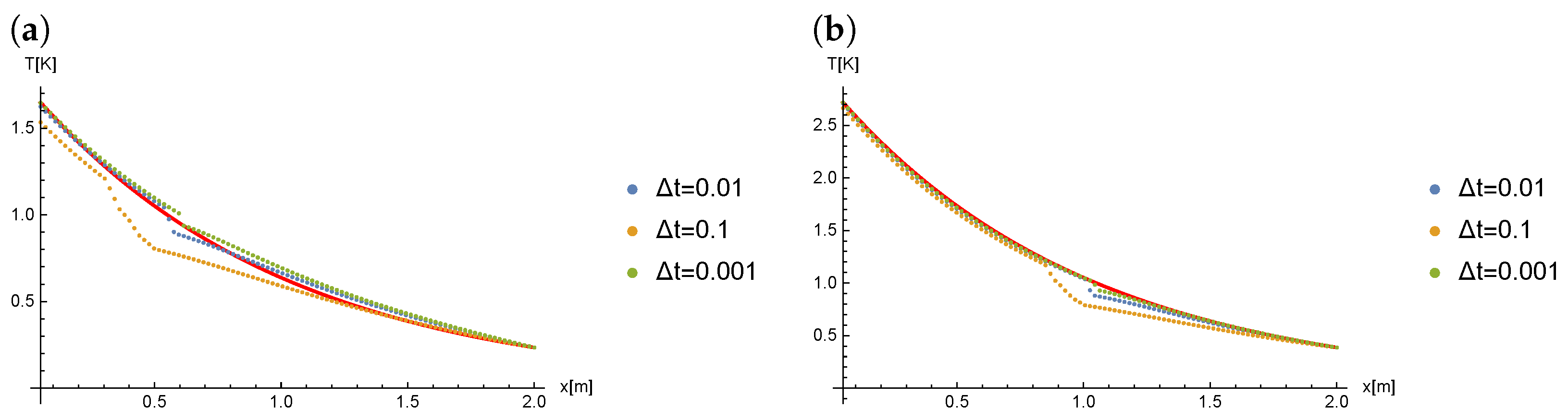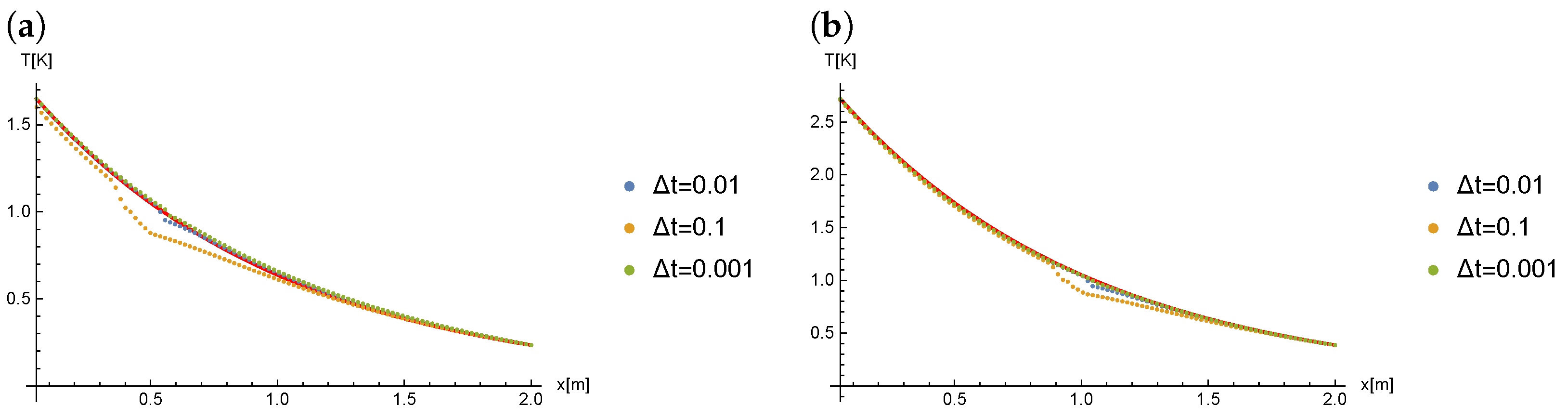Further reduction of the time step to the $\Delta t=0.001$ resulted in obtaining insignificantly smaller errors calculated for the whole area. 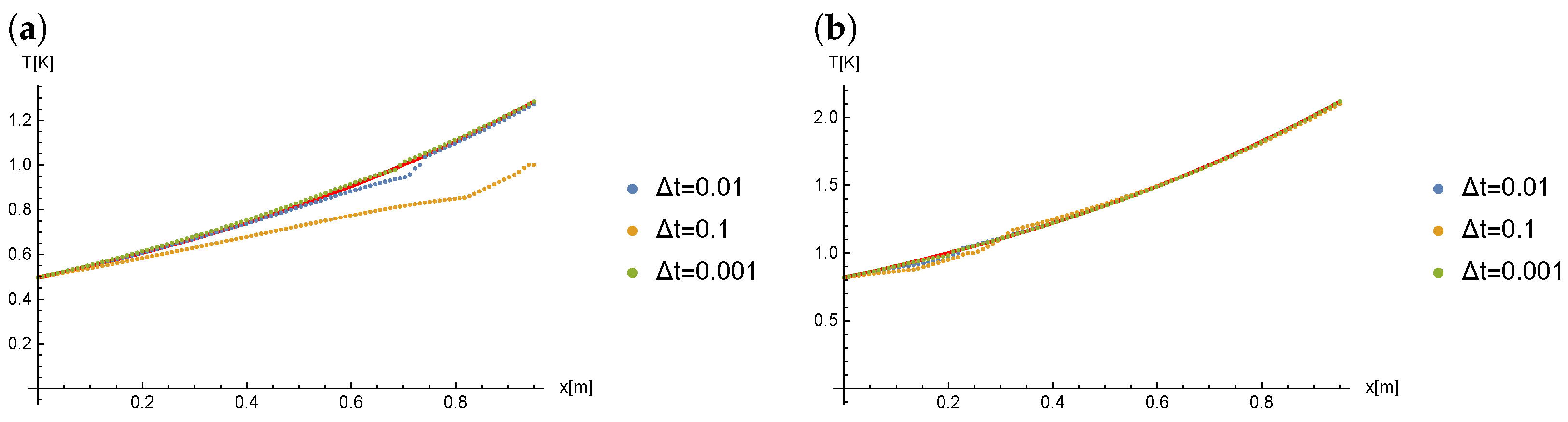In such a case, the greatest reduction of errors was obtained near the phases boundary (see Figure 2).

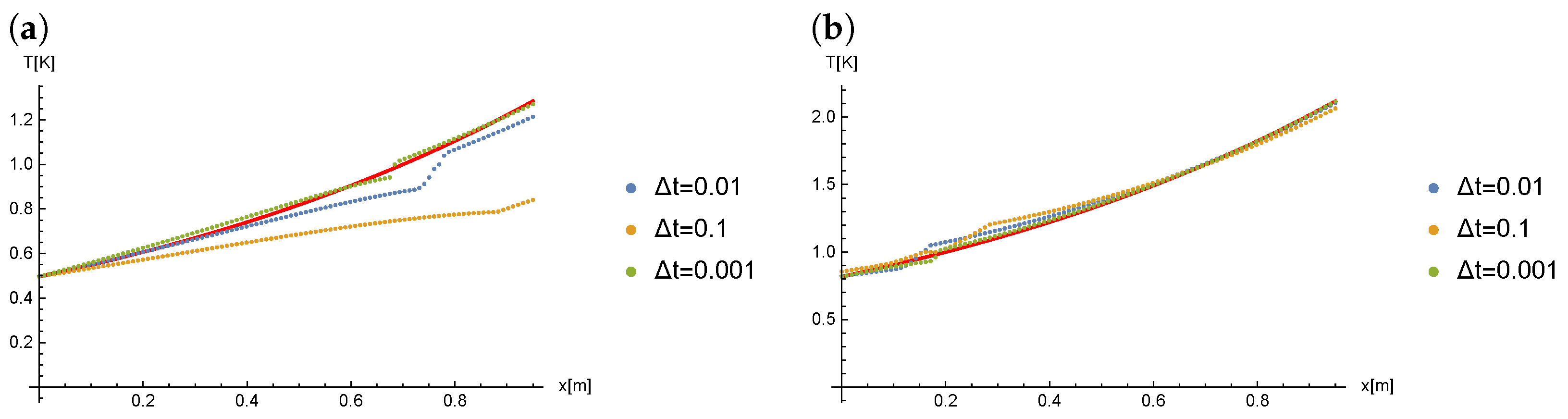
The Figure 2 presents the comparison of results for $N=100$ ($\Delta x=0.0195$) and for different values of $\Delta t$ in case when the Caputo derivative is of order $\alpha =0.5$.

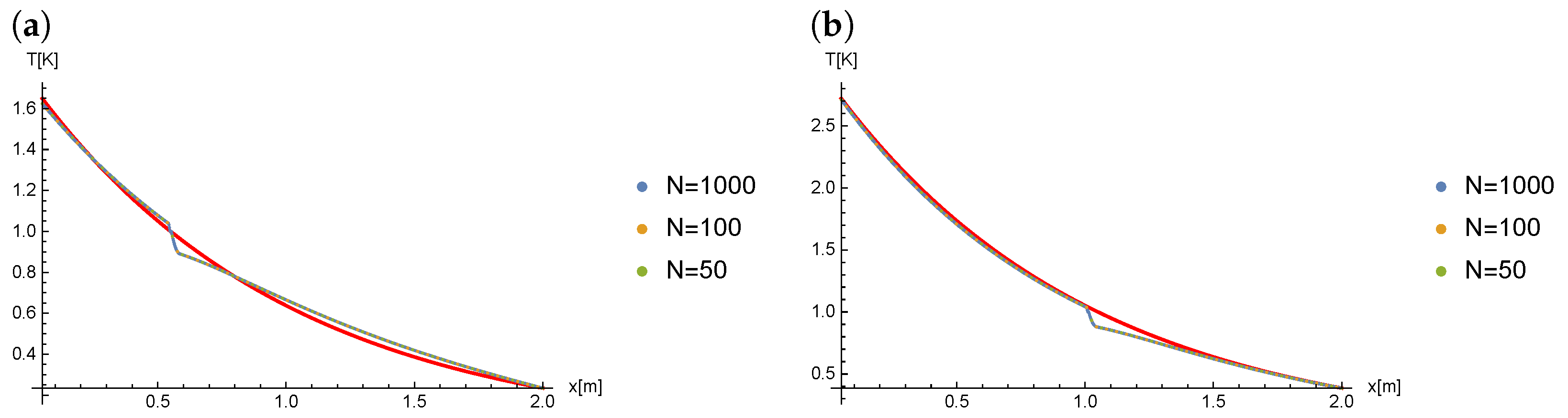
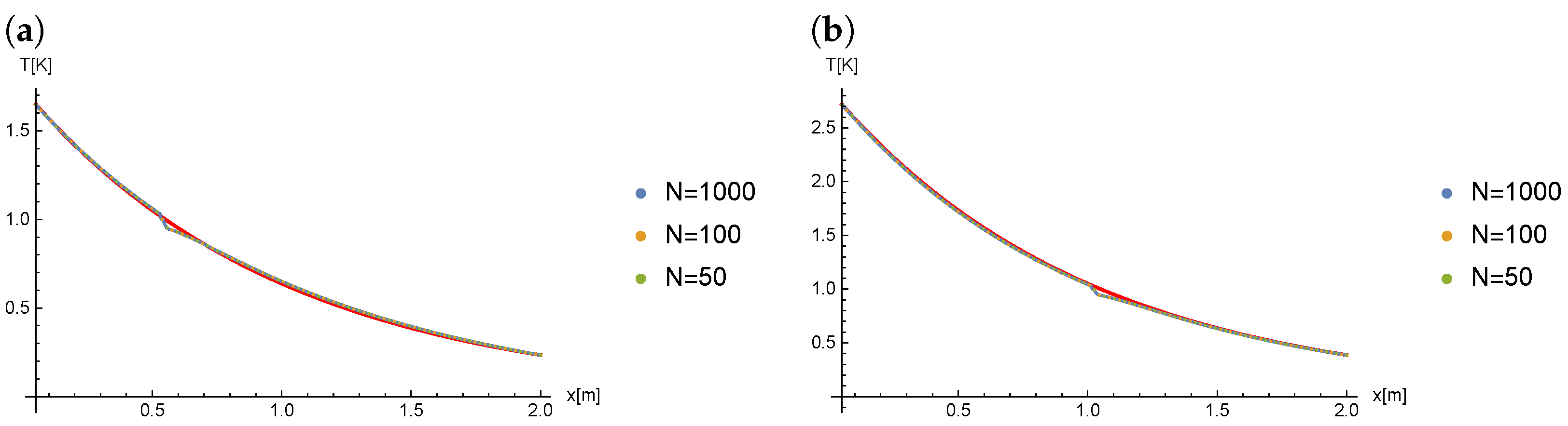
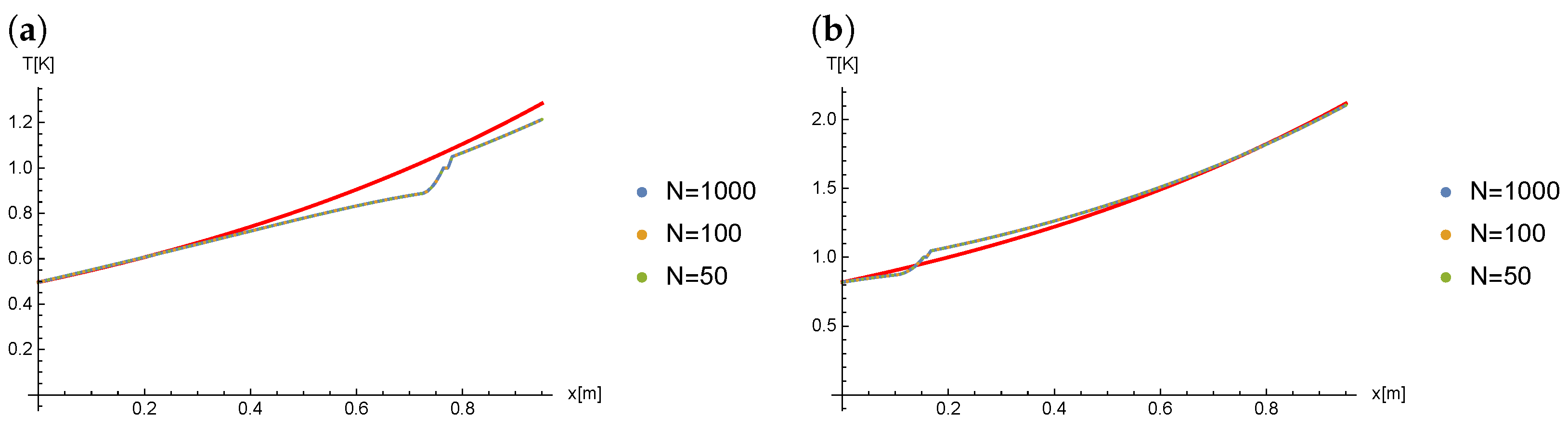
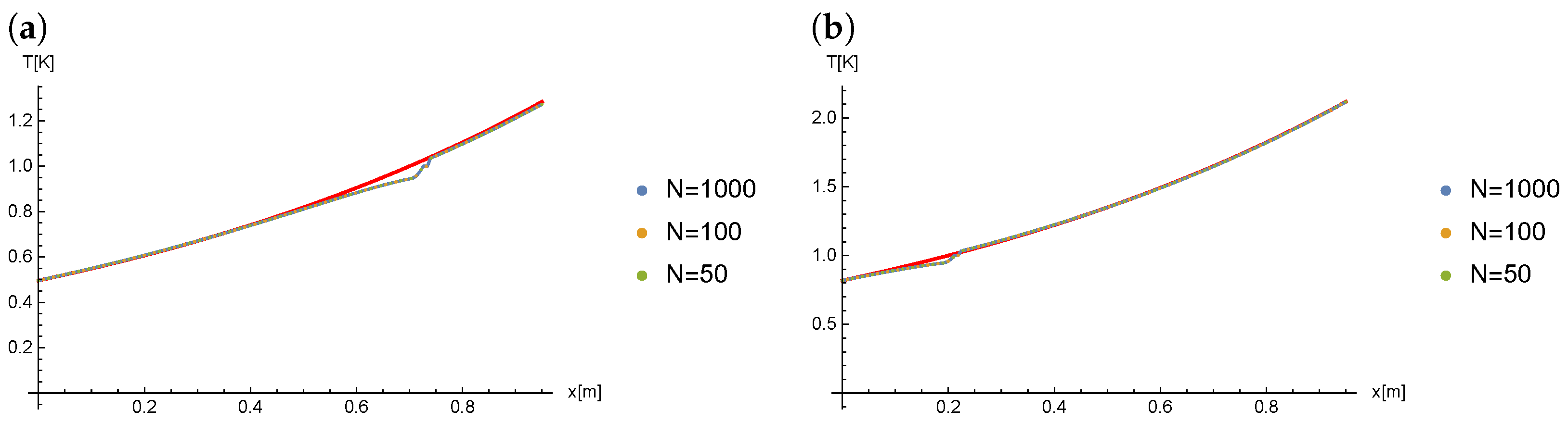
The Figure 3 shows the comparison of results for $\Delta t=0.01$ and for different values of N (therefore, different values of $\Delta x$) in case when the Caputo derivative is of the order $\alpha =0.5$.

The

Table 1. The mean and maximum absolute errors for $\alpha =0.3$ in Example 1.

		$\mathbf{\Delta }\mathit{t}=0.1$	$\mathbf{\Delta }\mathit{t}=0.01$
$N=50$	${\Delta }_{avg}$	0.101347	0.0472061
$\Delta x=0.039$	${\Delta }_{max}$	0.56382	0.411988
$N=100$	${\Delta }_{avg}$	0.101103	0.0469636
$\Delta x=0.0195$	${\Delta }_{max}$	0.563984	0.412356
$N=1000$	${\Delta }_{avg}$	0.100867	0.0467296
$\Delta x=0.00195$	${\Delta }_{max}$	0.56402	0.412448

shows the mean and maximum absolute errors of approximate solutions obtained for the different grid sizes and the order of Caputo derivative $\alpha =0.3$. The average error value obtained for all of the considered grid sizes does not exceed $0.11$. The smallest errors were obtained for the most dense grid.

The

Table 2. The mean and maximum absolute errors for $\alpha =0.5$ in Example 1.

		$\mathbf{\Delta }\mathit{t}=0.1$	$\mathbf{\Delta }\mathit{t}=0.01$
$N=50$	${\Delta }_{avg}$	0.0698689	0.0280351
$\Delta x=0.039$	${\Delta }_{max}$	0.467583	0.318906
$N=100$	${\Delta }_{avg}$	0.0697529	0.0279801
$\Delta x=0.0195$	${\Delta }_{max}$	0.467901	0.319516
$N=1000$	${\Delta }_{avg}$	0.0695975	0.0279169
$\Delta x=0.00195$	${\Delta }_{max}$	0.467987	0.319685

shows the mean and maximum absolute errors of approximate solutions obtained for the different grid sizes and the order of Caputo derivative $\alpha =0.5$. The average error does not exceed the value $0.07$. The best result was obtained for $\Delta t=0.01,$ for which the maximum error does not exceed the value $0.32$.

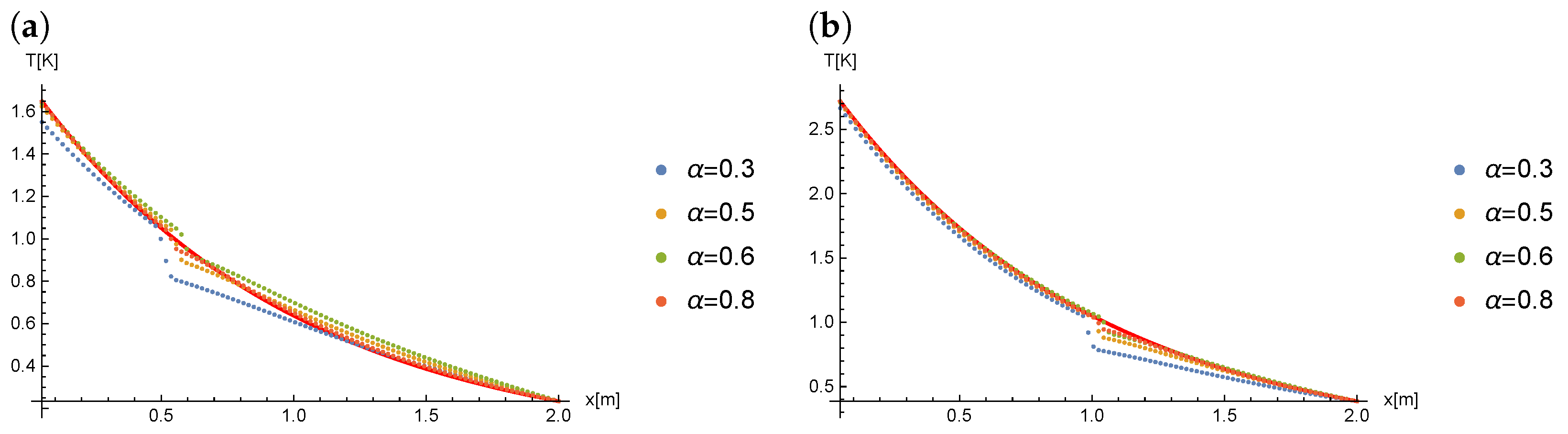
The Figure 4 presents a comparison of the obtained results for $\alpha =0.5$, $N=100$ ($\Delta x=0.0195$) and different values of $\Delta t$.

The Figure 5 presents a comparison of results for $N=100$ ($\Delta x=0.0195$) and different values of $\Delta t$ when the Caputo derivative is of order $\alpha =0.8$.

Figure 6 presents the comparison of the results for $\Delta t=0.01$ and for different values of N (therefore, different values of $\Delta x$) when the Caputo derivative is of order $\alpha =0.8$.

The

Table 3. The mean and maximum absolute errors for $\alpha =0.8$ in Example 1.

		$\mathbf{\Delta }\mathit{t}=0.1$	$\mathbf{\Delta }\mathit{t}=0.01$
$N=50$	${\Delta }_{avg}$	0.0411779	0.0102665
$\Delta x=0.039$	${\Delta }_{max}$	0.365232	0.222018
$N=100$	${\Delta }_{avg}$	0.0411296	0.0102742
$\Delta x=0.0195$	${\Delta }_{max}$	0.365862	0.223924
$N=1000$	${\Delta }_{avg}$	0.041078	0.0102558
$\Delta x=0.00195$	${\Delta }_{max}$	0.366067	0.224544

shows the mean and maximum absolute errors of approximate solutions obtained for the different grid sizes and the order of Caputo derivative $\alpha =0.8$. In this case, the best result was also obtained for $\Delta t=0.01,$ for which the maximum error does not exceed $0.23$. The average error for each size of the grid, for which the calculation was performed, does not exceed the value $0.042$. While thickening the time grid ($\Delta t=0.001$), the maximum error values decrease to $0.15$, while the average error values stay at a similar level.

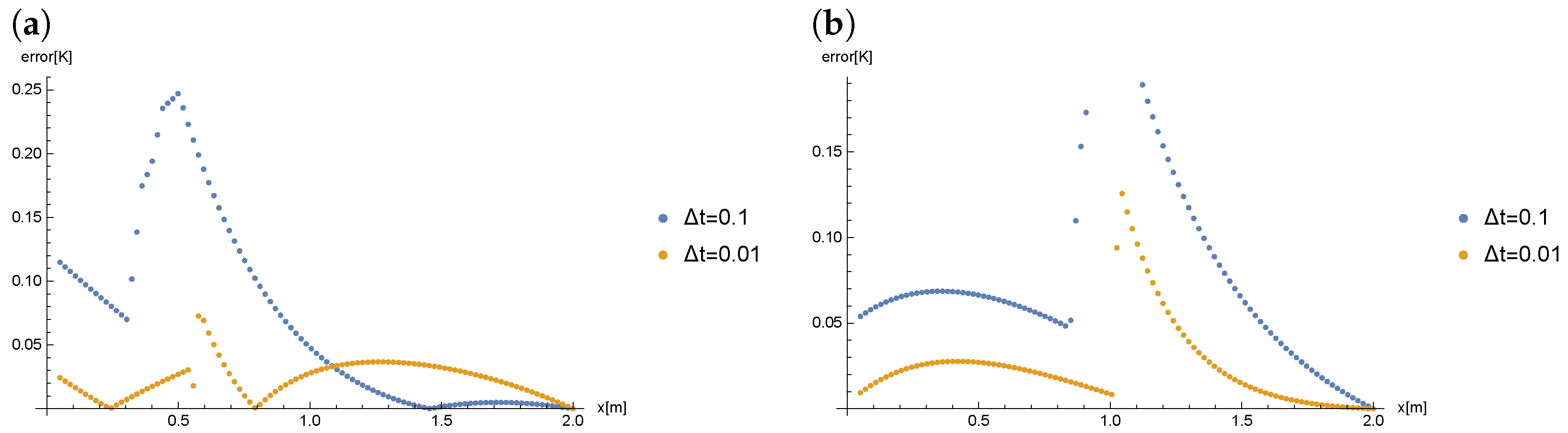
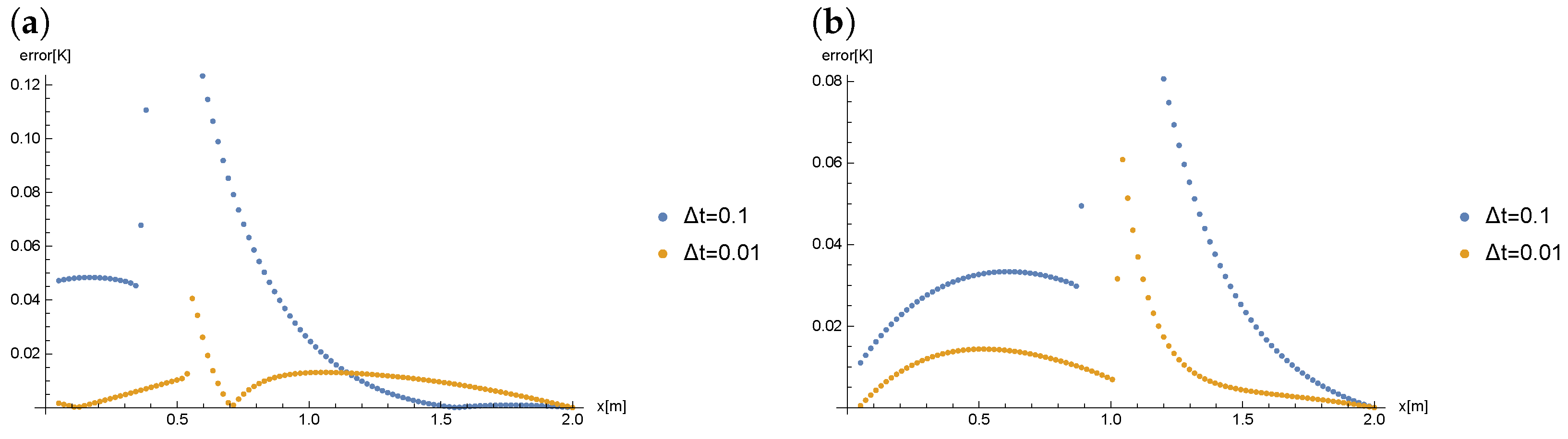
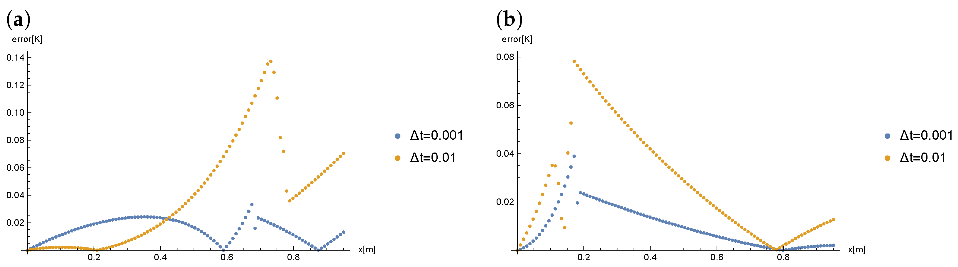
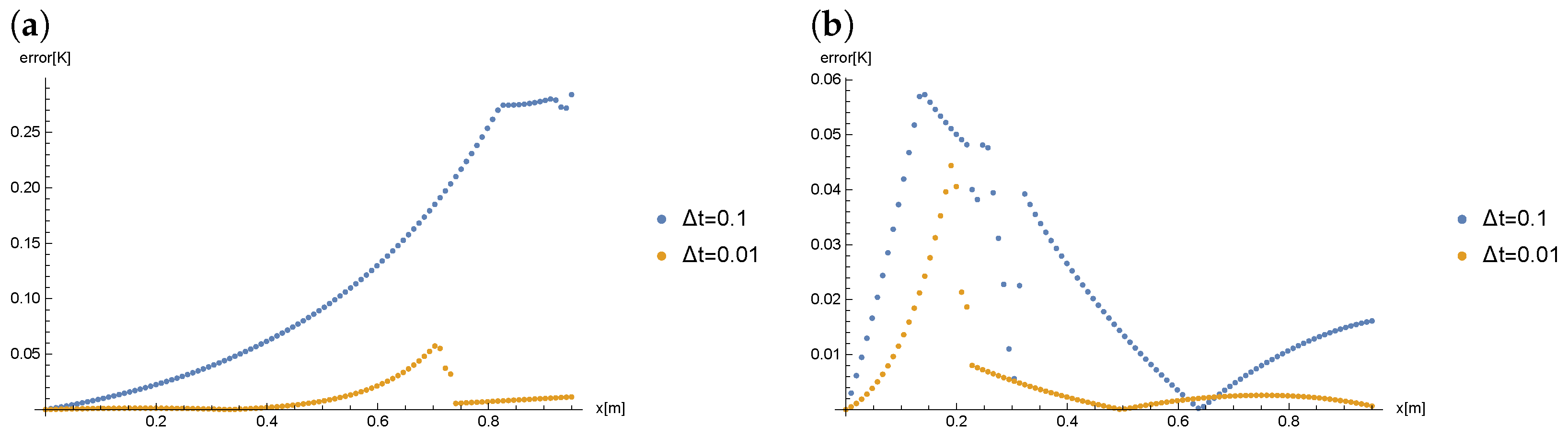
The Figure 7 presents the comparison of errors obtained for $\alpha =0.8$, $N=100$ ($\Delta x=0.0195$) and the different values of $\Delta t$.

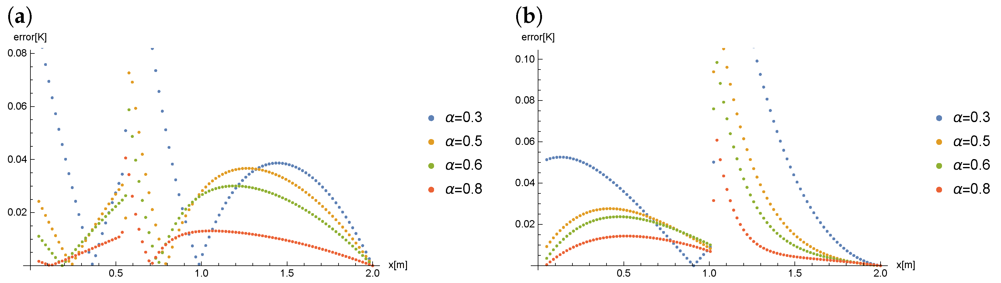
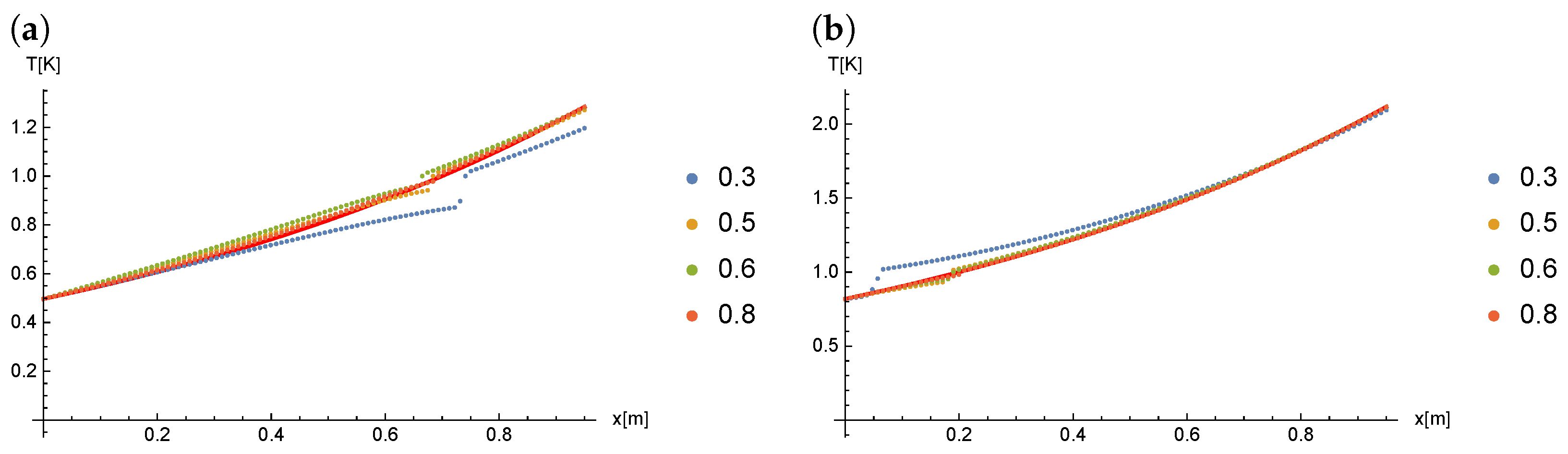
The results obtained for the parameters $\Delta t=0.01$, $N=100$ ($\Delta x=0.0195$) were compared depending on the order $\alpha$ of the derivative. Figure 8 presents a comparison of the results obtained for $N=100$ ($\Delta x=0.0195$), $\Delta t=0.01$ and for the different orders $\alpha$ of the Caputo derivative.

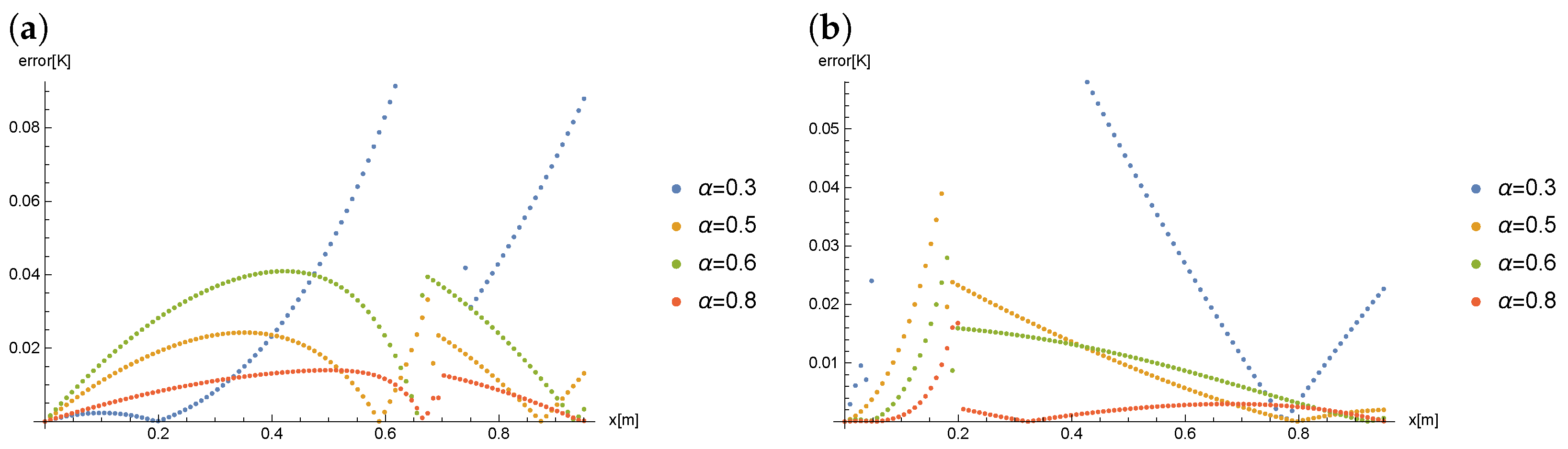
The Figure 9 presents the comparison of the errors obtained for the different values of order of derivative $\alpha$ for the parameters $\Delta t=0.01$ and $N=100$.

7. Numerical Example 2

We consider the melting process described by the model (1)–(7). This time, the melting process is happening from the right side. Let $x\in [0,0.95]$ and $t\in [0,1.5]$. Moreover, we assume the following values: ${\overline{\lambda }}_S=125$, ${\overline{\lambda }}_L=130$, ${\overline{a}}_S={\overline{a}}_L=\frac{1}{2}$, $T_m=1$. The initial temperature at time $t=0$ is described by the function

$$T_0\left(x\right)=e^{x-0.95}.$$

On the boundaries, we set the boundary conditions of the first kind

$$T_z\left(t\right)=e^{0.5t-0.95},$$

$$T_b\left(t\right)=e^{0.5t}.$$

Right-hand limit of enthalpy at point $T_m$ varies over time and depends on the time-dependent function $\kappa \left(t\right)$. The form of function $\kappa \left(t\right)$ depends on the order of the Caputo derivative

$$\kappa \left(t\right)=(1-\alpha )\frac{({\overline{\lambda }}_L-{\overline{\lambda }}_S)\mathrm{\Gamma }(1-\alpha )}{{\overline{a}}_L{(t+0.1)}^{1-\alpha }}.$$

The exact solution of such stated problem is defined by the functions

$$T_L(x,t)=e^{0.5t-0.95+x},$$

$$T_S(x,t)=e^{0.5t-0.95+x}.$$

To solve this problem, the described above alternating phase truncation method was used. The average and maximum errors presented in the tables were calculated for the whole region $\mathrm{\Omega }=[0,0.95]\times [0,1.5]$. The calculations were performed for the different grid sizes. The space area was divided into $N=50$, $N=100$ and $N=1000$ parts, which corresponds to the step along the spatial axis being equal to $\Delta x=0.019$, $\Delta x=0.0095$ and $\Delta x=0.00095$, respectively. For the simpler notation, the spatial coordinate discretization will be later identified by N. The time step was equal to the following values: $\Delta t=0.1$, $\Delta t=0.01$ and $\Delta t=0.001$.

The Figure 10 presents the comparison of solutions obtained for $N=100$ ($\Delta x=0.0095$) and for different values of $\Delta t$ in case of the Caputo derivative order $\alpha =0.5$.

The Figure 11 presents the comparison of results obtained for $\Delta t=0.01$ and for different values of N (thereby different values of $\Delta x$) in case of the Caputo derivative order $\alpha =0.5$.

The

Table 4. The mean and maximum absolute errors for $\alpha =0.3$ in Example 2.

		$\mathbf{\Delta }\mathit{t}=0.1$	$\mathbf{\Delta }\mathit{t}=0.01$	$\mathbf{\Delta }\mathit{t}=0.001$
$N=50$	${\Delta }_{avg}$	0.125054	0.0810909	0.0427681
$\Delta x=0.019$	${\Delta }_{max}$	0.551399	0.429743	0.338091
$N=100$	${\Delta }_{avg}$	0.124846	0.0809066	0.0426732
$\Delta x=0.0095$	${\Delta }_{max}$	0.551438	0.429812	0.338181
$N=1000$	${\Delta }_{avg}$	0.124673	0.0807353	0.0425803
$\Delta x=0.00095$	${\Delta }_{max}$	0.551459	0.429831	0.338208

shows the mean and maximum absolute errors of approximate solutions obtained for the different grid sizes and the Caputo derivative order $\alpha =0.3$. The average error value does not exceed $0.126$. The best results were obtained for $\Delta t=0.001$, for which the average error does not exceed $0.043$ and the maximum error does not exceed $0.339$. It can be observed that decreasing step along the spatial axis has little impact on an improvement of the results. The differences arise most probably from the rounding errors. The differences are more significant for the smaller number of nodes (for example, for $N=10$).

The

Table 5. The mean and maximum absolute errors for $\alpha =0.5$ in Example 2.

		$\mathbf{\Delta }\mathit{t}=0.1$	$\mathbf{\Delta }\mathit{t}=0.01$	$\mathbf{\Delta }\mathit{t}=0.001$
$N=50$	${\Delta }_{avg}$	0.0947457	0.0380964	0.0172353
$\Delta x=0.019$	${\Delta }_{max}$	0.466191	0.328678	0.252733
$N=100$	${\Delta }_{avg}$	0.0946874	0.0380056	0.0172403
$\Delta x=0.0095$	${\Delta }_{max}$	0.466244	0.32881	0.252972
$N=1000$	${\Delta }_{avg}$	0.094633	0.0379193	0.0172308
$\Delta x=0.00095$	${\Delta }_{max}$	0.466273	0.328848	0.253048

shows the mean and maximum absolute errors of approximate solutions obtained for different grid sizes and the Caputo derivative order $\alpha =0.5$. The best results were obtained for $\Delta t=0.001$, for which the maximum error value is lower than $0.256$ for each case of the considered size of the grid along the spatial coordinate. The lowest value of average error, not exceeding $0.018$, was obtained for $\Delta t=0.001$.

The Figure 12 presents the comparison of errors obtained for $\alpha =0.5$, $N=100$ ($\Delta x=0.0095$) and different values of $\Delta t$.

The Figure 13 presents the comparison of results obtained for $N=100$ ($\Delta x=0.0095$) and different values of $\Delta t$ in cases when the Caputo derivative is of order $\alpha =0.8$.

The Figure 14 presents the comparison of results obtained for $\Delta t=0.01$ and different values of N (thus, different values of $\Delta x$) when the Caputo derivative is of order $\alpha =0.8$.

The

Table 6. The mean and maximum absolute errors for $\alpha =0.8$ in Example 2.

		$\mathbf{\Delta }\mathit{t}=0.1$	$\mathbf{\Delta }\mathit{t}=0.01$	$\mathbf{\Delta }\mathit{t}=0.001$
$N=50$	${\Delta }_{avg}$	0.0650444	0.0138944	0.006421
$\Delta x=0.019$	${\Delta }_{max}$	0.365781	0.224542	0.143035
$N=100$	${\Delta }_{avg}$	0.065094	0.0138906	0.00646026
$\Delta x=0.0095$	${\Delta }_{max}$	0.365927	0.224989	0.144328
$N=1000$	${\Delta }_{avg}$	0.0651208	0.0138655	0.00648839
$\Delta x=0.00095$	${\Delta }_{max}$	0.365976	0.225133	0.144768

shows the mean and maximum absolute errors of approximate solutions obtained for the different grid sizes and the Caputo derivative order $\alpha =0.8$. The best result was obtained for $\Delta t=0.001$, for which the maximum and average error values were both the lowest. For each considered grid size, the average error does not exceed $0.066$.

Figure 15 presents the comparison of the errors obtained for $\alpha =0.8$, $N=100$ ($\Delta x=0.0095$) and different values of $\Delta t$.

The results obtained for the parameters $\Delta t=0.001$, $N=100$ ($\Delta x=0.0095$) were compared depending on the Caputo derivative order $\alpha$. Figure 16 presents the results of this comparison.

Table 7. The mean and maximum absolute errors for $\Delta t=0.001$, $N=100$ ($\Delta x=0.0095$) and different values of the Caputo derivative order $\alpha$ in Example 2.

		$\mathit{\alpha }=0.3$	$\mathit{\alpha }=0.5$	$\mathit{\alpha }=0.6$	$\mathit{\alpha }=0.8$
$t=0.5$	${\Delta }_{avg}$	0.042691	0.0148576	0.0259057	0.0085936
	${\Delta }_{max}$	0.151112	0.0332324	0.0409613	0.0139867
$t=1$	${\Delta }_{avg}$	0.0249003	0.0113576	0.0154067	0.00444684
	${\Delta }_{max}$	0.101183	0.0355406	0.0304888	0.0107901
$t=1.5$	${\Delta }_{avg}$	0.051743	0.00975133	0.00854907	0.00229658
	${\Delta }_{max}$	0.144233	0.0389485	0.0279889	0.0168211

collects the mean and maximum absolute errors of the approximate solutions obtained for $N=100$, $\Delta t=0.001$, and different values of the Caputo derivative order $\alpha$. For all of the considered moments of time t, the lowest mean and maximum errors were obtained for $\alpha =0.8$.

Figure 17 presents the comparison of errors obtained for $\Delta t=0.001$, $N=100$ ($\Delta x=0.0095$) and different values of the Caputo derivative order $\alpha$.

8. Conclusions

In this article, the one-dimensional two-phase direct Stefan problem was considered with the derivative with respect to time defined as the fractional derivative of the Caputo type. The aim of the article was to propose the approximate method for solving the fractional Stefan problem. The alternating phase truncation method adapted to the equations with the fractional derivative of Caputo type was used for this purpose. The numerical examples show that the presented algorithm for the properly chosen grid in the domain of space and time allows us to determine the good approximate temperature distribution in the considered region. In both examples, the best choice of the grid size was the grid of the time step $\Delta t=0.001$ and $N=100$ nodes in the domain of space. In case of the Caputo derivative order $\alpha =0.5$, the maximum absolute errors did not exceed $0.08$. The best solutions were obtained for the order of derivative $\alpha =0.8$. The obtained results incline us to conduct further research on the application of the alternating phase truncation method to solve the fractional Stefan problem.

In the current paper, the APT method was applied for the time-fractional Stefan problem. In the future, the application for space-fractional Stefan problem can be considered. Other plans concern the generalization of the method for the multidimensional case and its application for solving the inverse fractional Stefan problem.