Author Contributions
Conceptualization, Y.W. and G.H.; Data curation, Y.W., L.H. and G.H.; Formal analysis, L.H. and J.Z.; Funding acquisition, G.H.; Investigation, Y.W., L.H. and J.Z.; Methodology, L.H., J.Z. and G.H.; Project administration, Y.W., J.Z. and G.H.; Resources, Y.W. and G.H.; Software, Y.W., L.H. and J.Z.; Supervision, G.H.; Validation, J.Z. and G.H.; Visualization, G.H.; Writing–original draft, Y.W., L.H., J.Z. and G.H.; Writing—review & editing, Y.W., L.H., J.Z. and G.H. All authors have read and agreed to the published version of the manuscript.
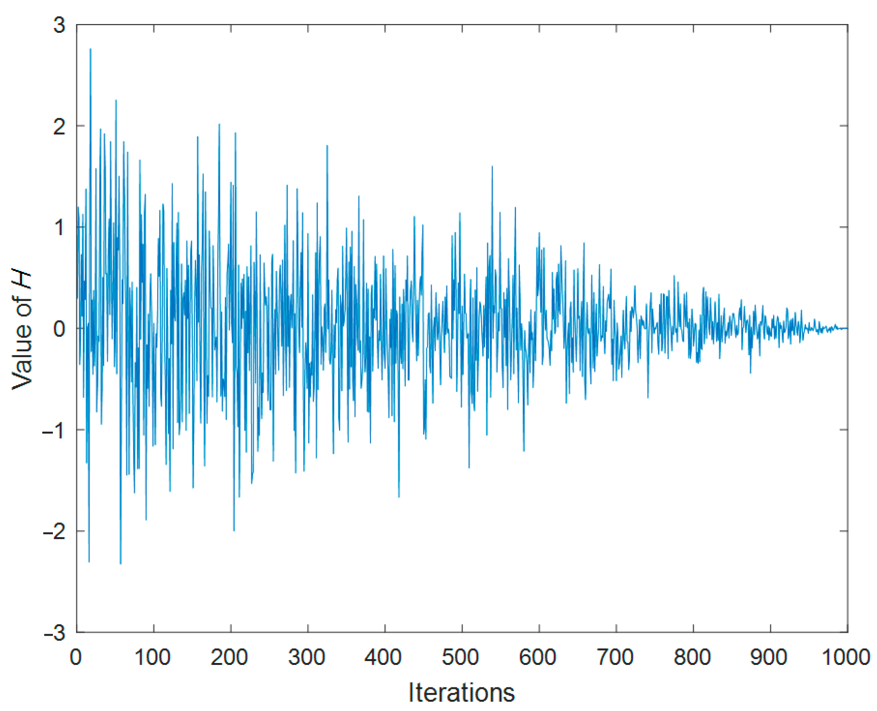
Figure 1.
The change of H over the course of 1000 iterations.
Figure 1.
The change of H over the course of 1000 iterations.
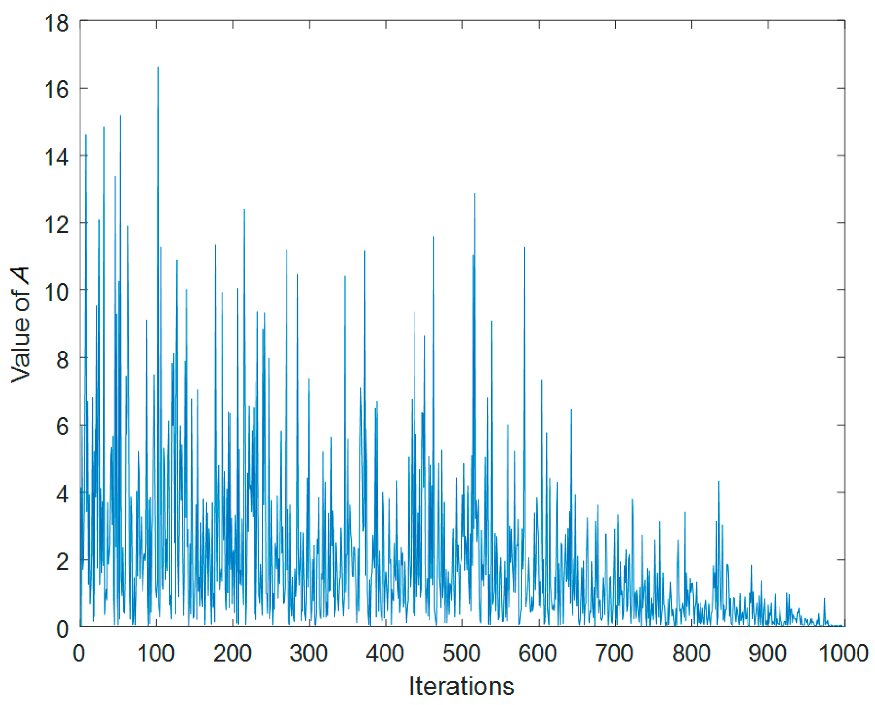
Figure 2.
The change of A over the course of 1000 iterations.
Figure 2.
The change of A over the course of 1000 iterations.
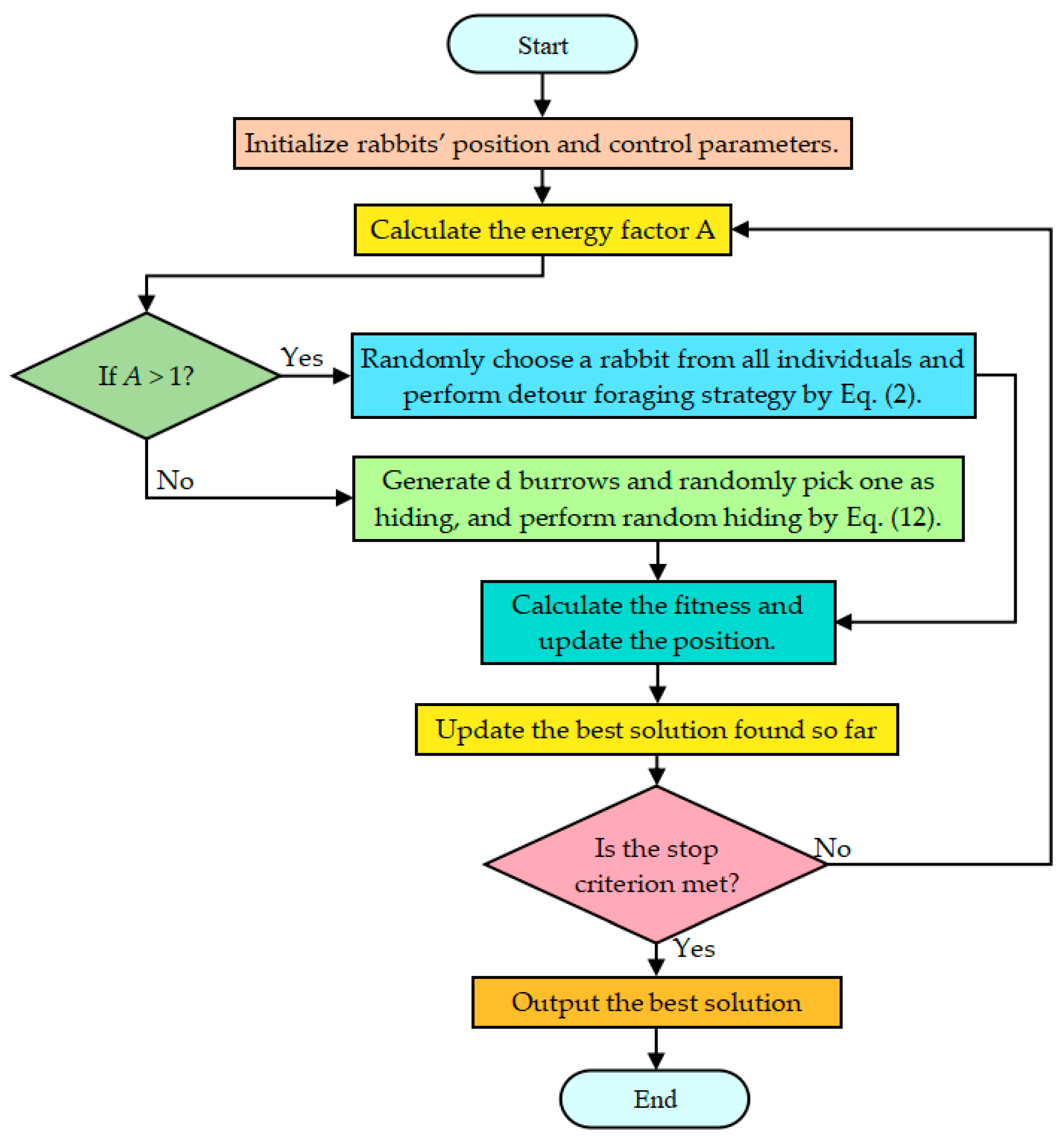
Figure 3.
Flow chart of ARO.
Figure 3.
Flow chart of ARO.
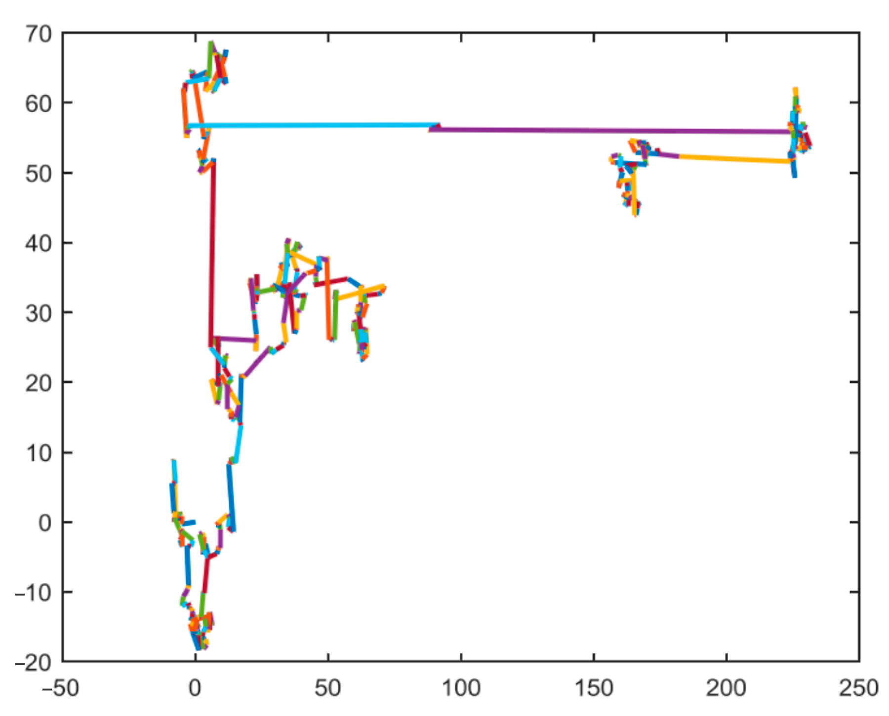
Figure 4.
Lévy flight path of 500 times movements in a two-dimensional space.
Figure 4.
Lévy flight path of 500 times movements in a two-dimensional space.
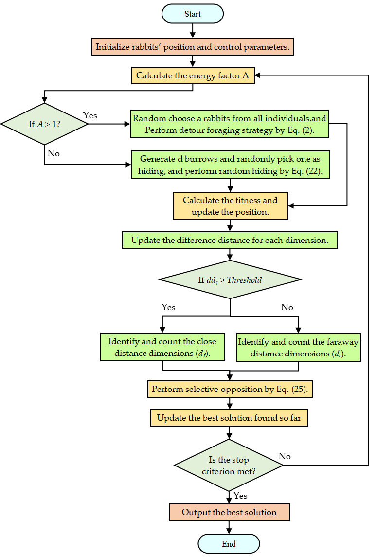
Figure 5.
Flowchart for the LARO algorithm.
Figure 5.
Flowchart for the LARO algorithm.
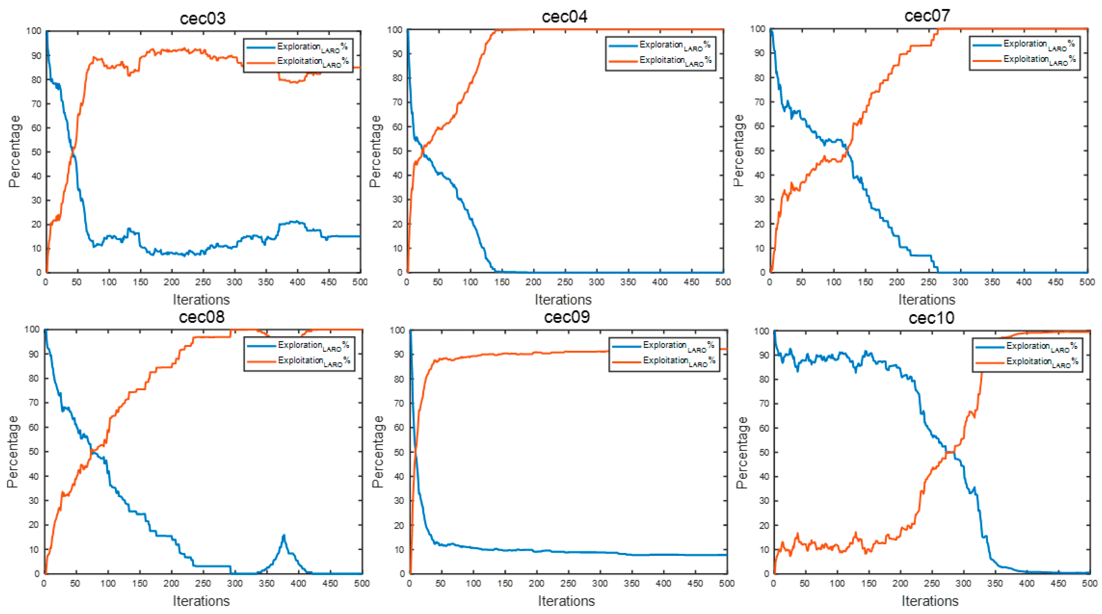
Figure 6.
The exploration and exploitation diagrams of LARO.
Figure 6.
The exploration and exploitation diagrams of LARO.
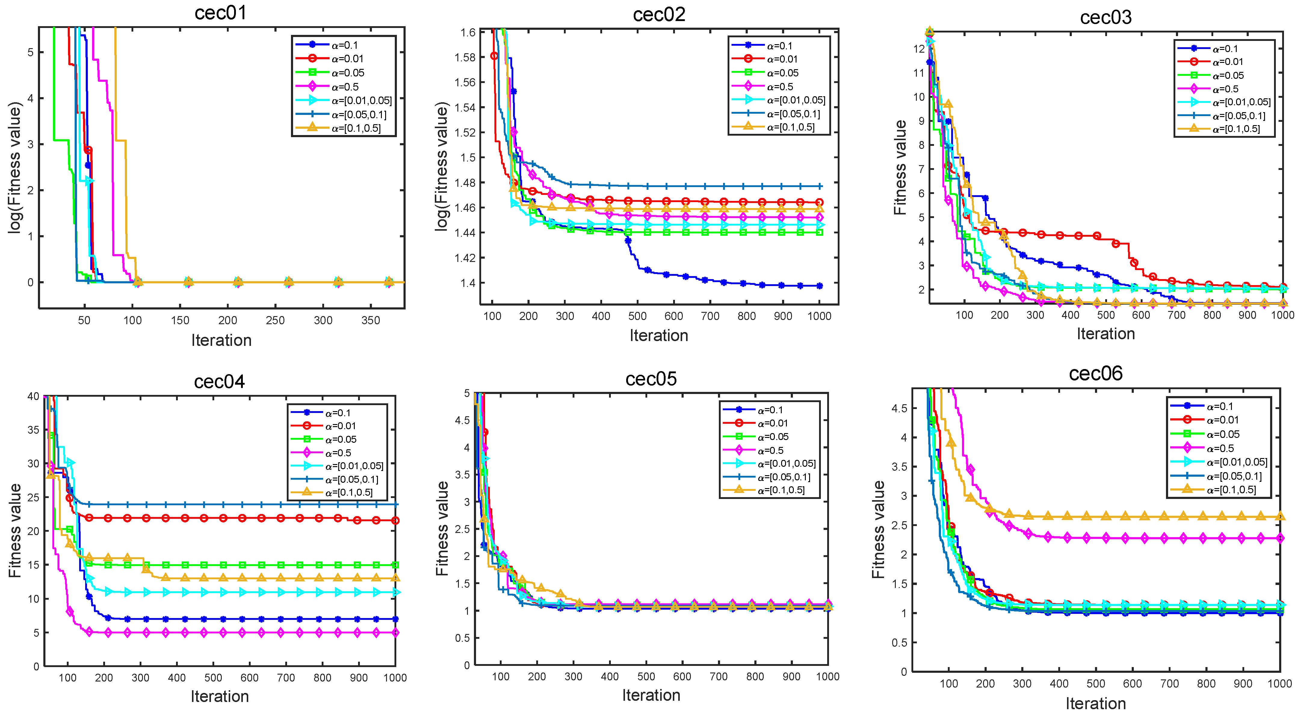
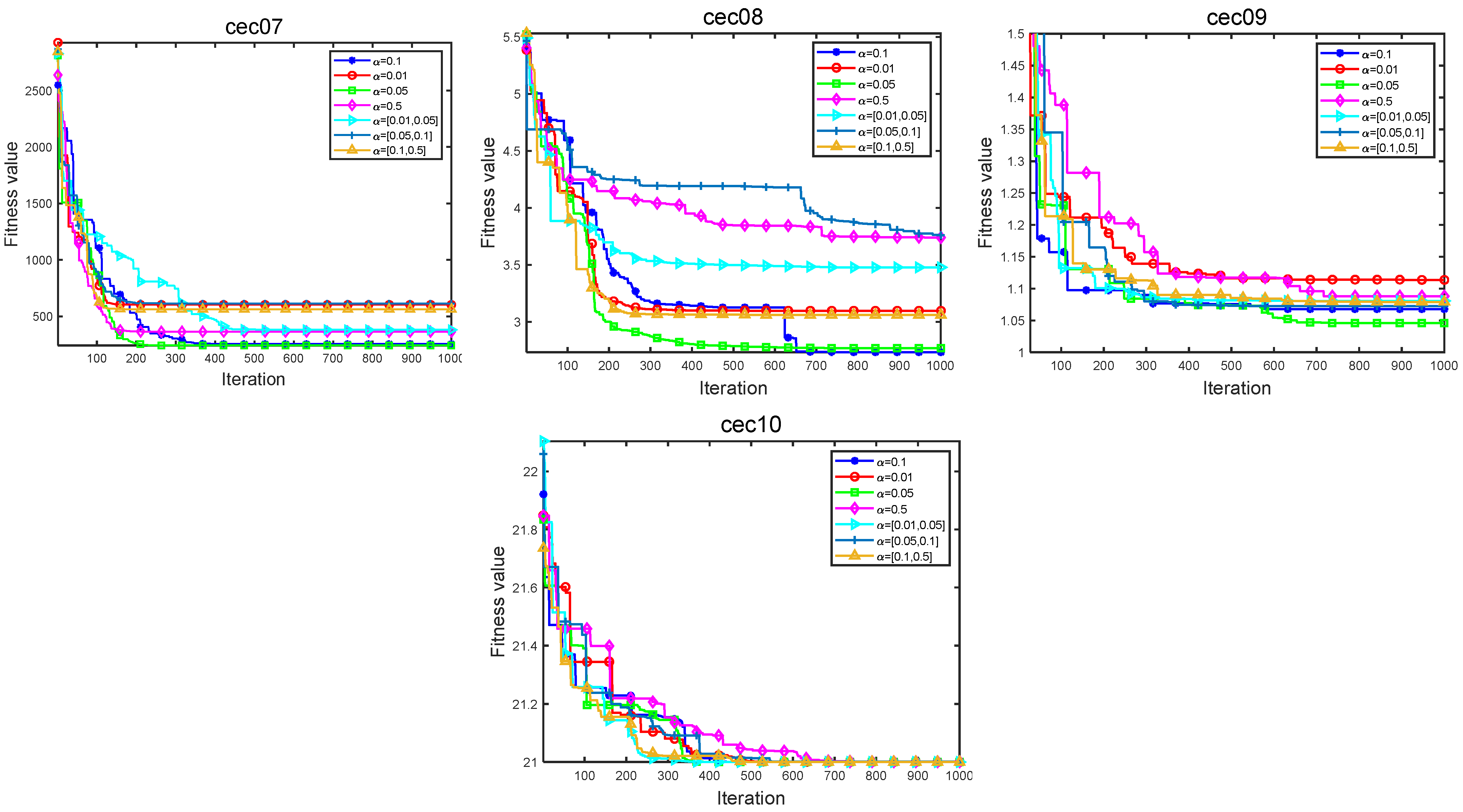
Figure 7.
Iteration plot of seven parameters in CEC2019.
Figure 7.
Iteration plot of seven parameters in CEC2019.
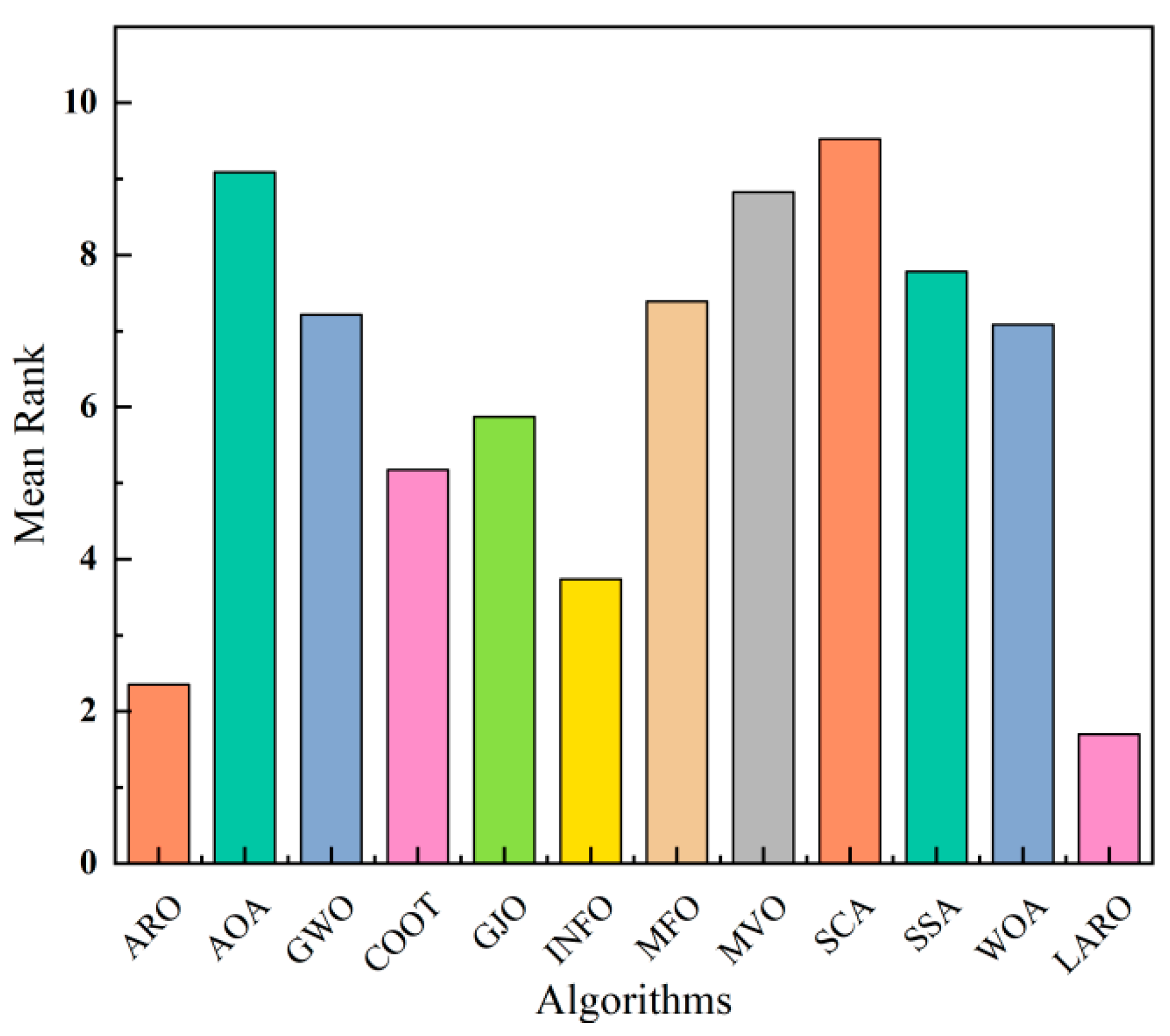
Figure 8.
The average rank of the twelve algorithms.
Figure 8.
The average rank of the twelve algorithms.
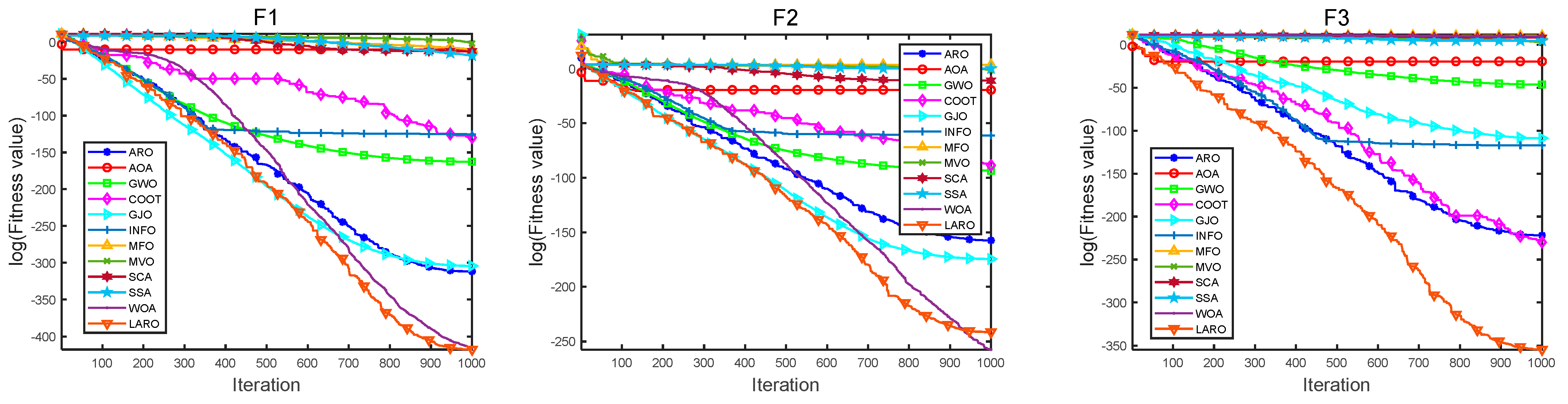
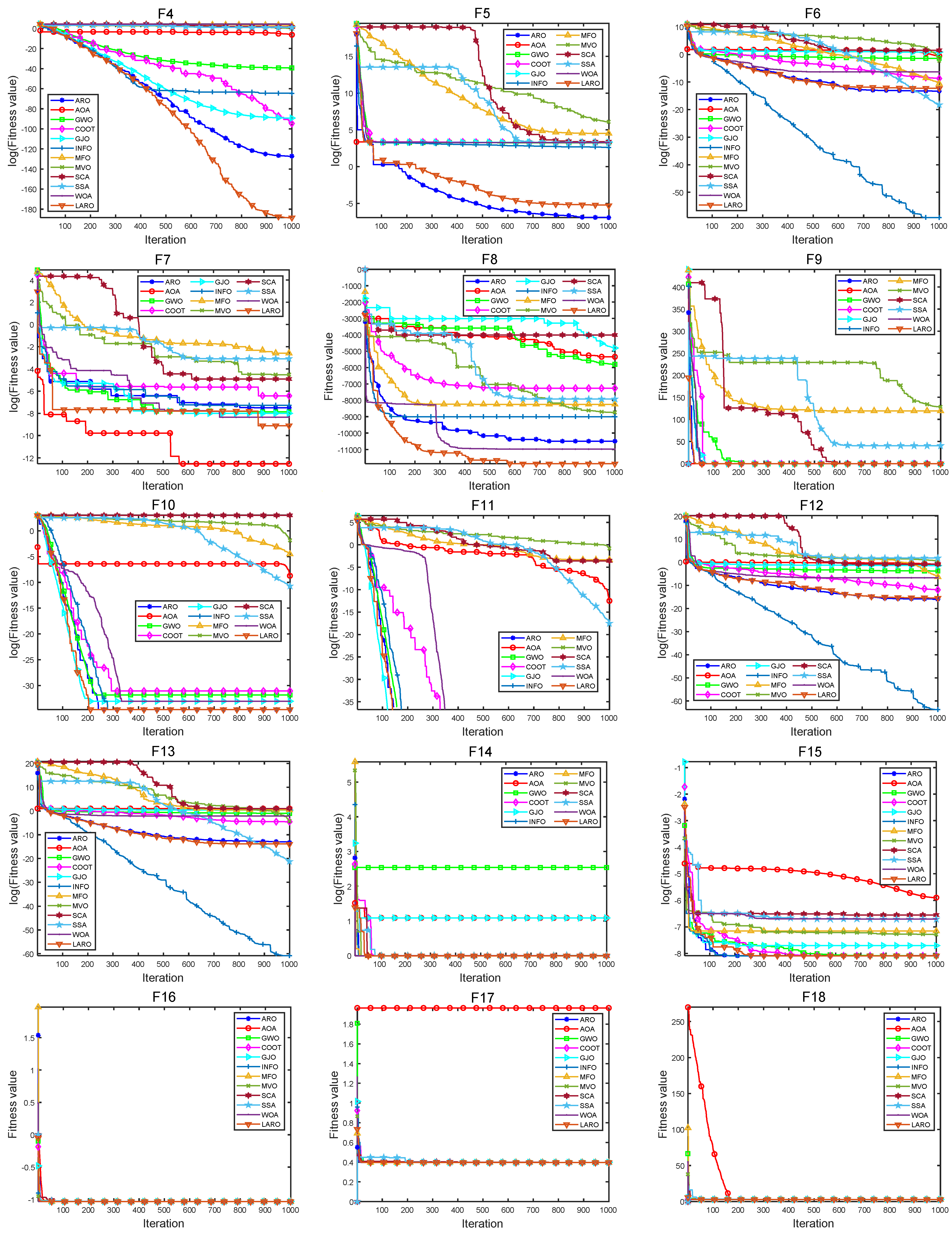
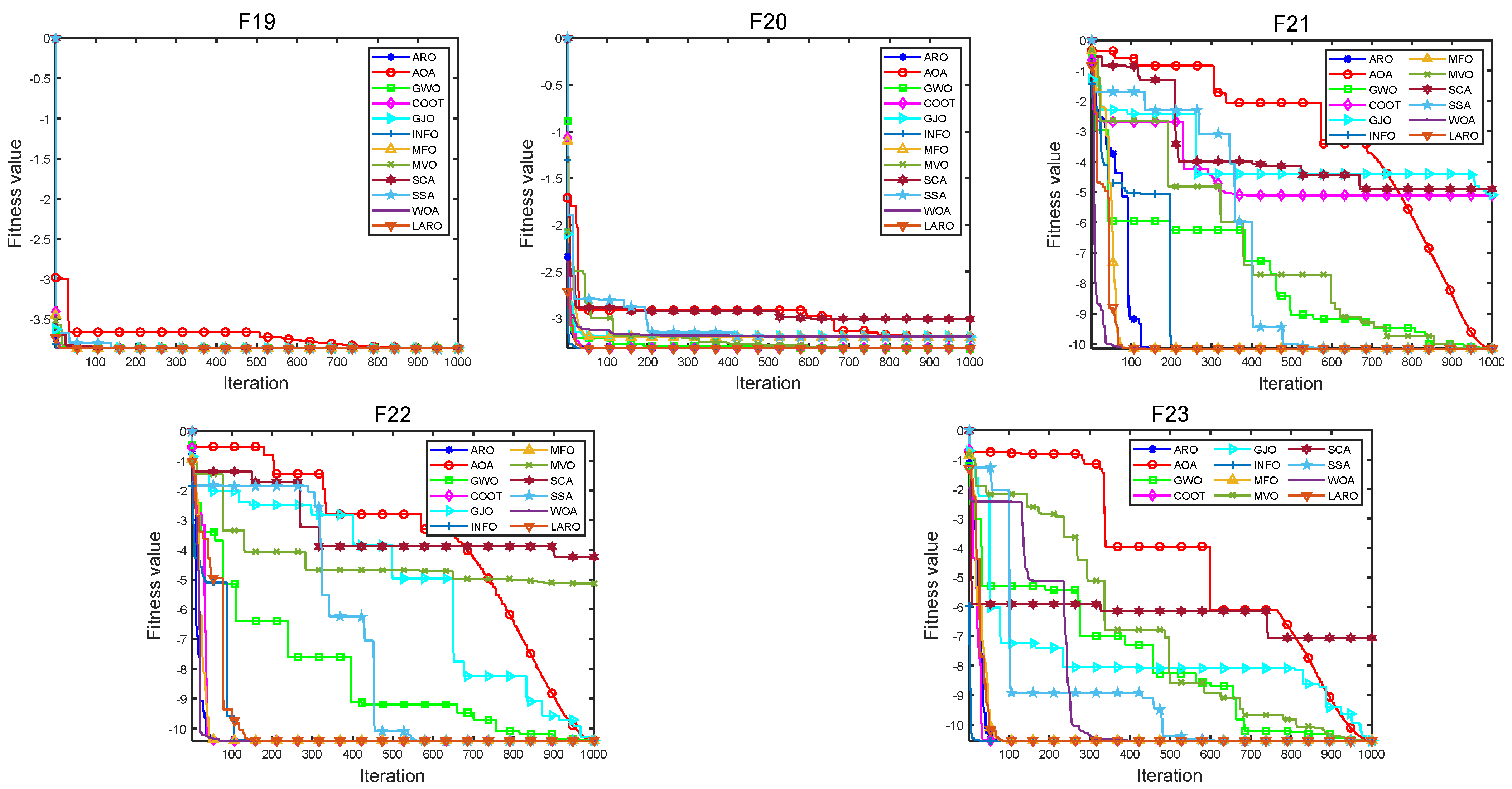
Figure 9.
Convergence plots of LARO and different MH methods on 23 test functions.
Figure 9.
Convergence plots of LARO and different MH methods on 23 test functions.
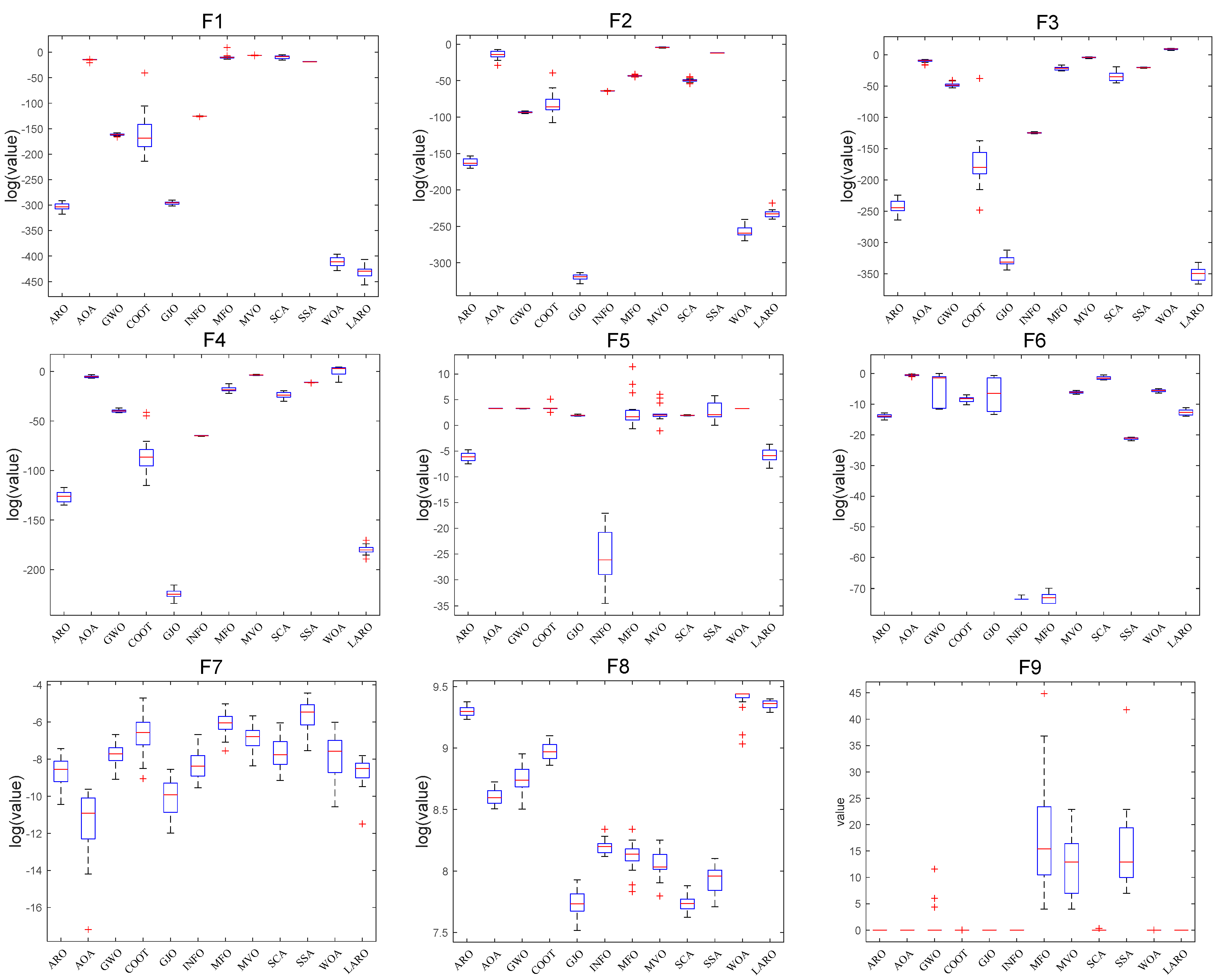
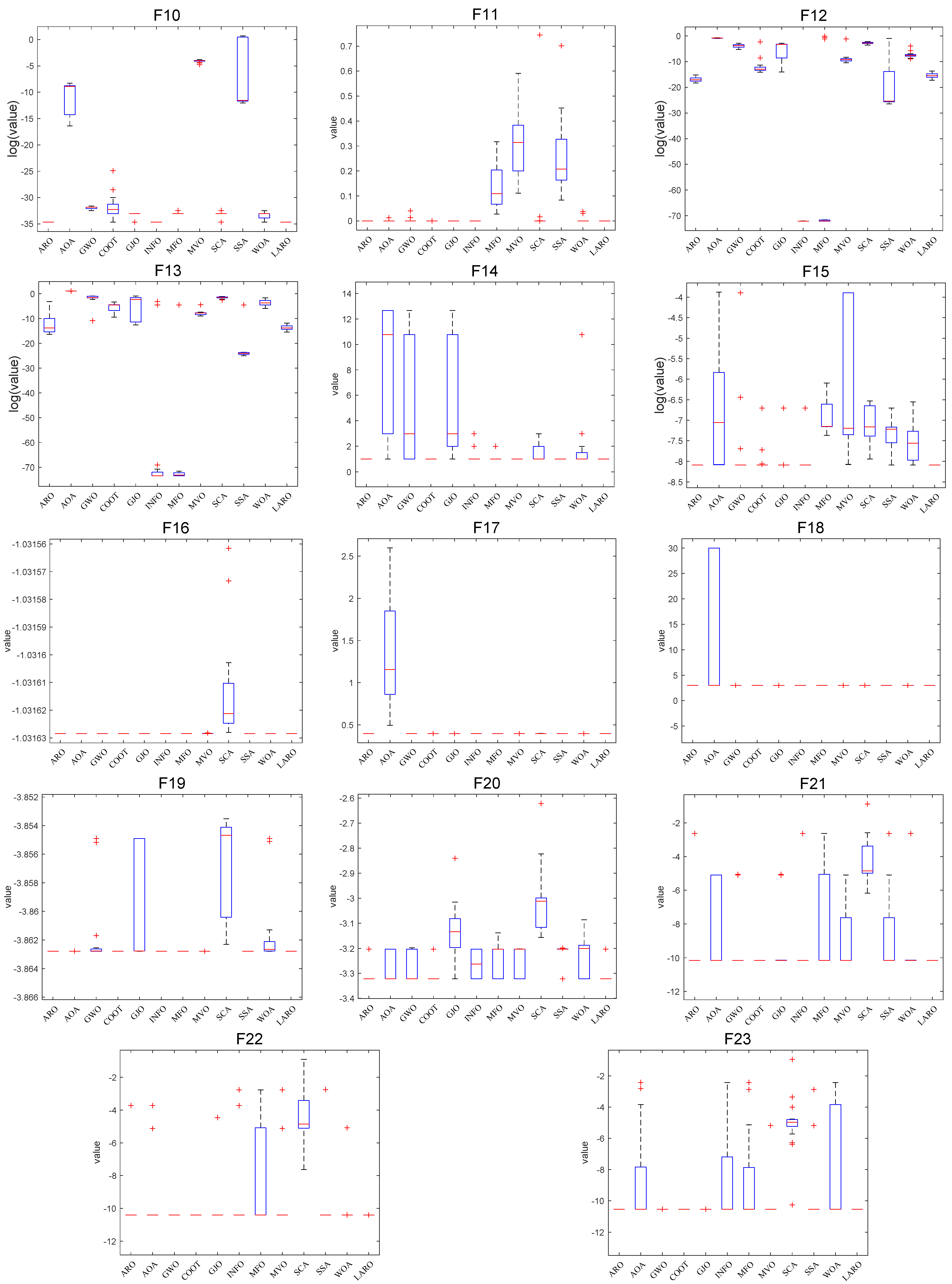
Figure 10.
Box plot of LARO and ARO, AOA, GWO, COOT, GJO, INFO, MFO, MVO, SCA, SSA, WOA on 23 test functions.
Figure 10.
Box plot of LARO and ARO, AOA, GWO, COOT, GJO, INFO, MFO, MVO, SCA, SSA, WOA on 23 test functions.
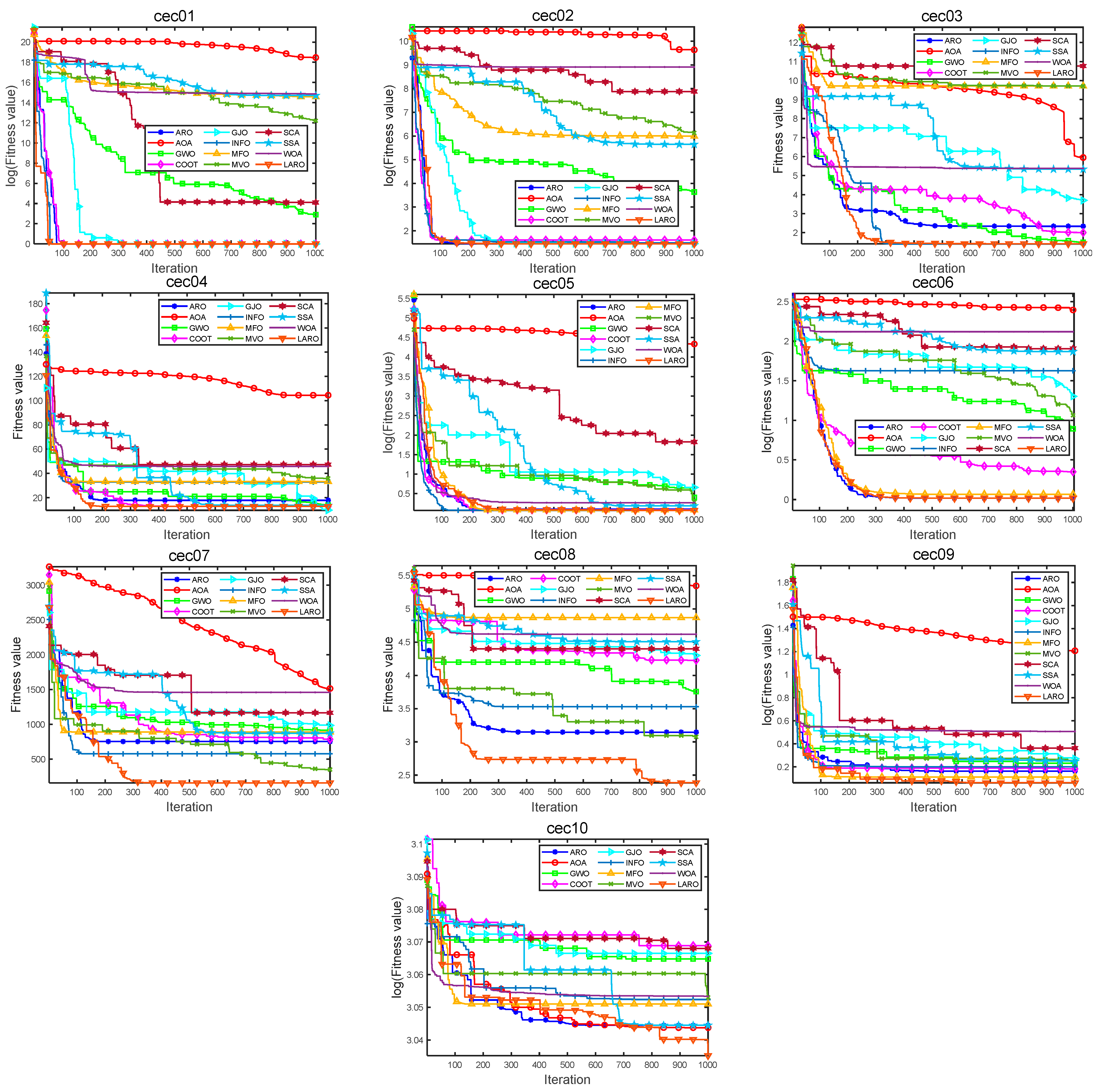
Figure 11.
Convergence plots of LARO and other search methods on the CEC2019 test functions.
Figure 11.
Convergence plots of LARO and other search methods on the CEC2019 test functions.
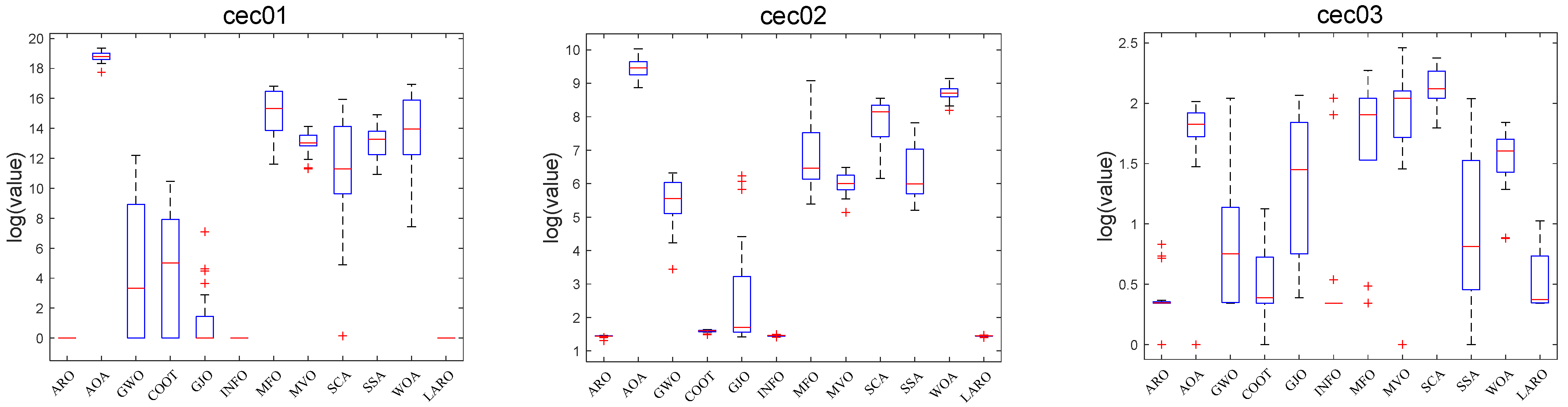
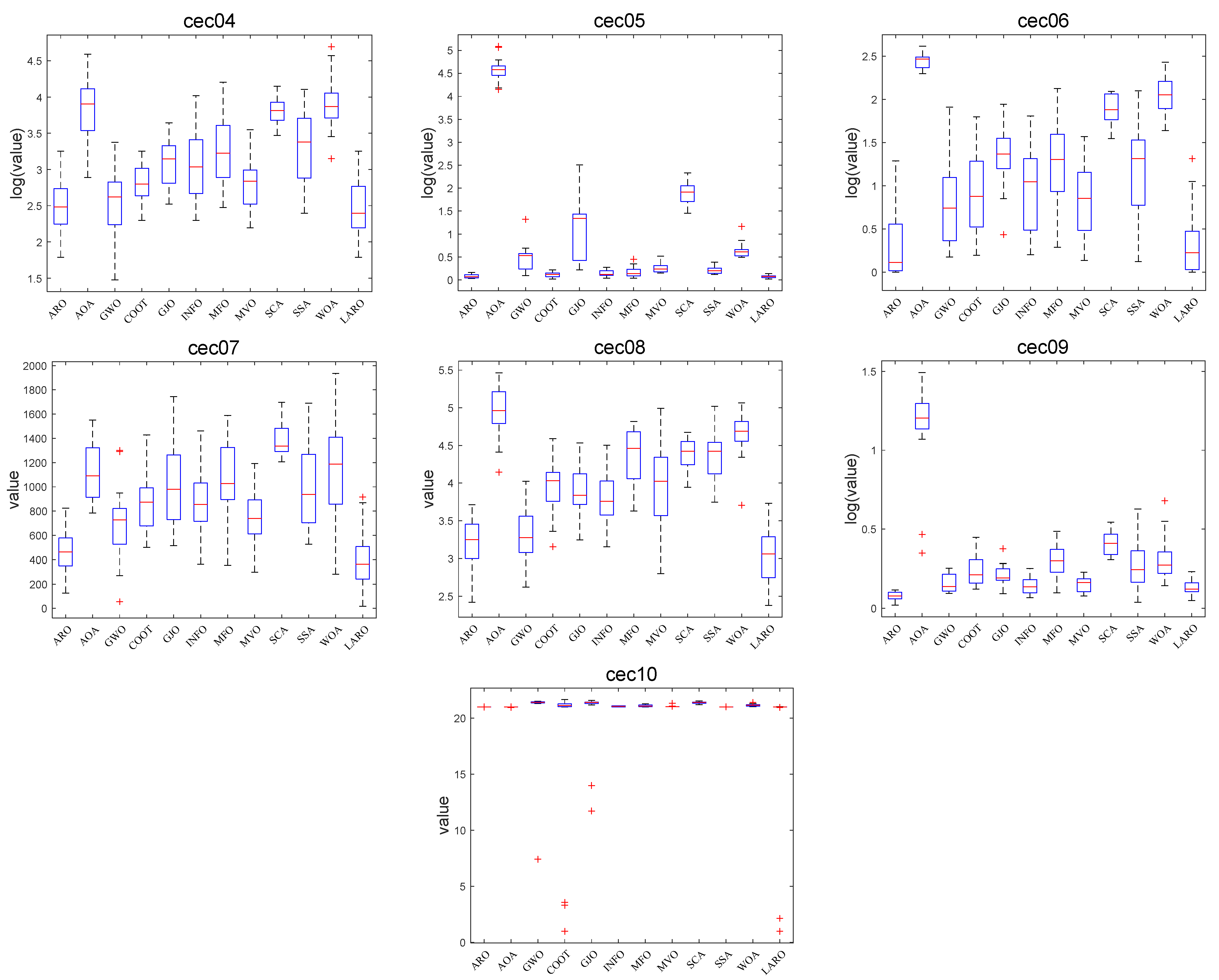
Figure 12.
Box plot of LARO and ARO, AOA, GWO, COOT, GJO, INFO, MFO, MVO, SCA, SSA, WOA on CEC2019 test functions.
Figure 12.
Box plot of LARO and ARO, AOA, GWO, COOT, GJO, INFO, MFO, MVO, SCA, SSA, WOA on CEC2019 test functions.
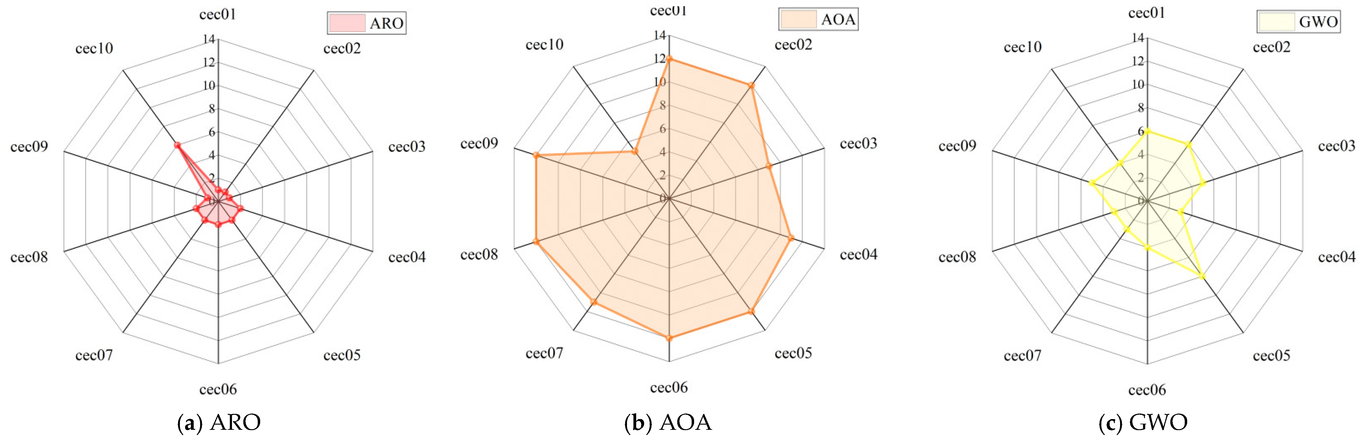
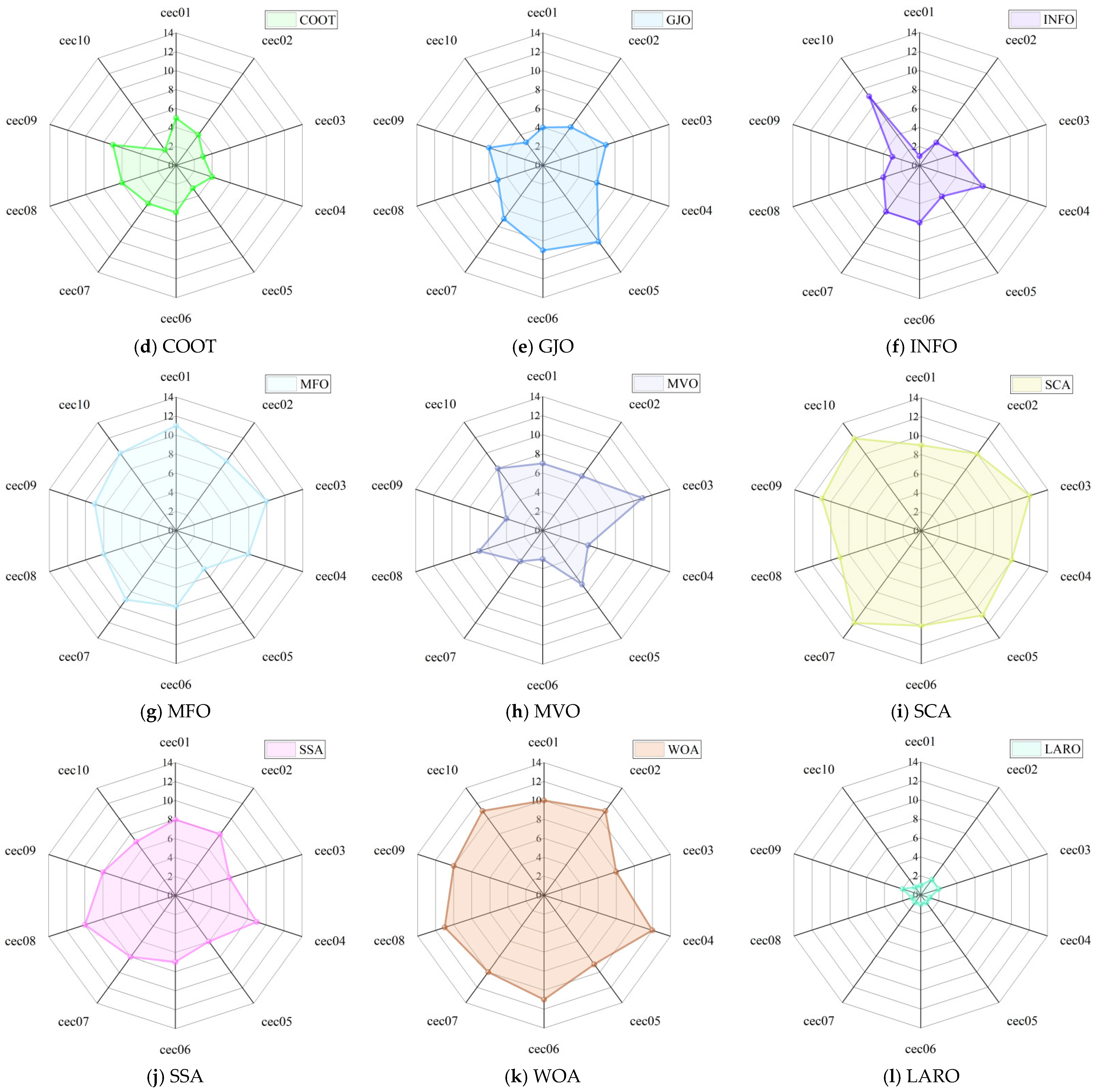
Figure 13.
Radar chart of ARO, AOA, GWO, COOT, GJO, INFO, MFO, MVO, SCA, SSA, WOA, and LARPO on CEC2019.
Figure 13.
Radar chart of ARO, AOA, GWO, COOT, GJO, INFO, MFO, MVO, SCA, SSA, WOA, and LARPO on CEC2019.
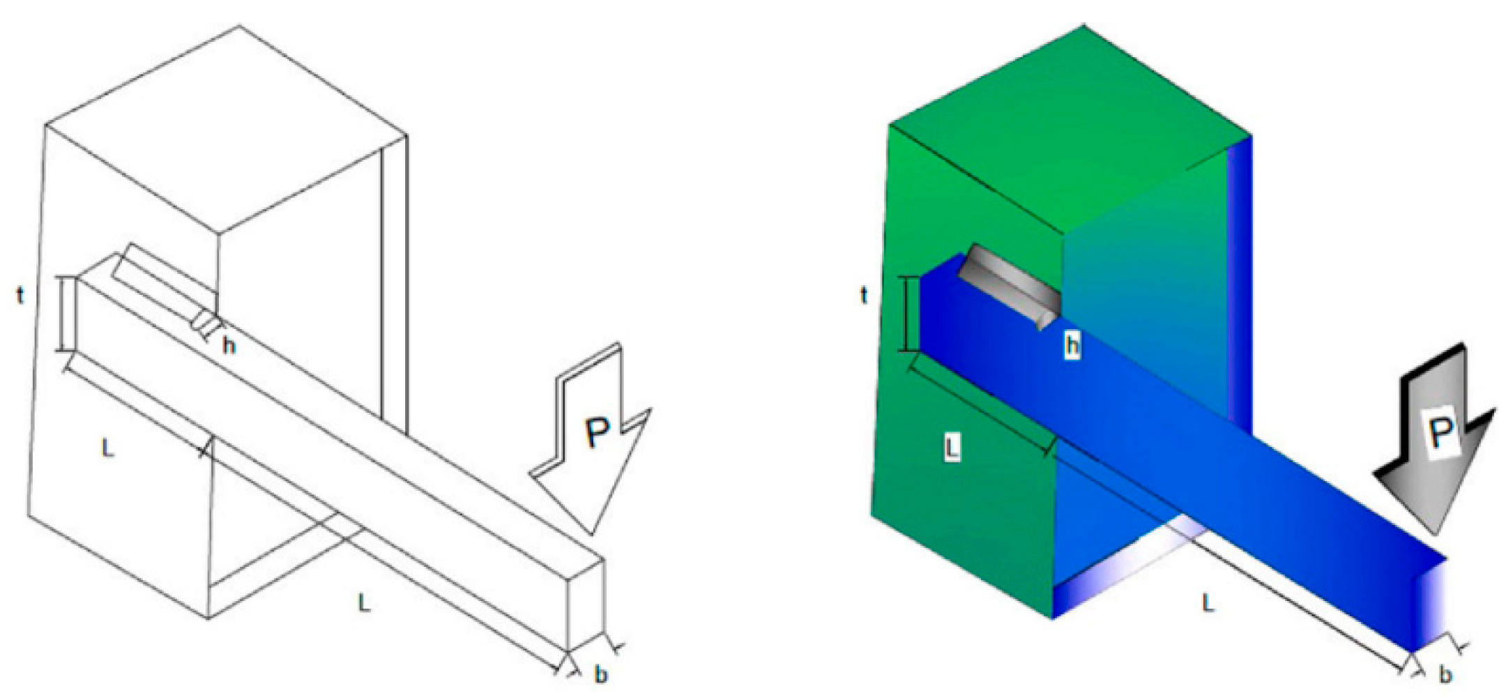
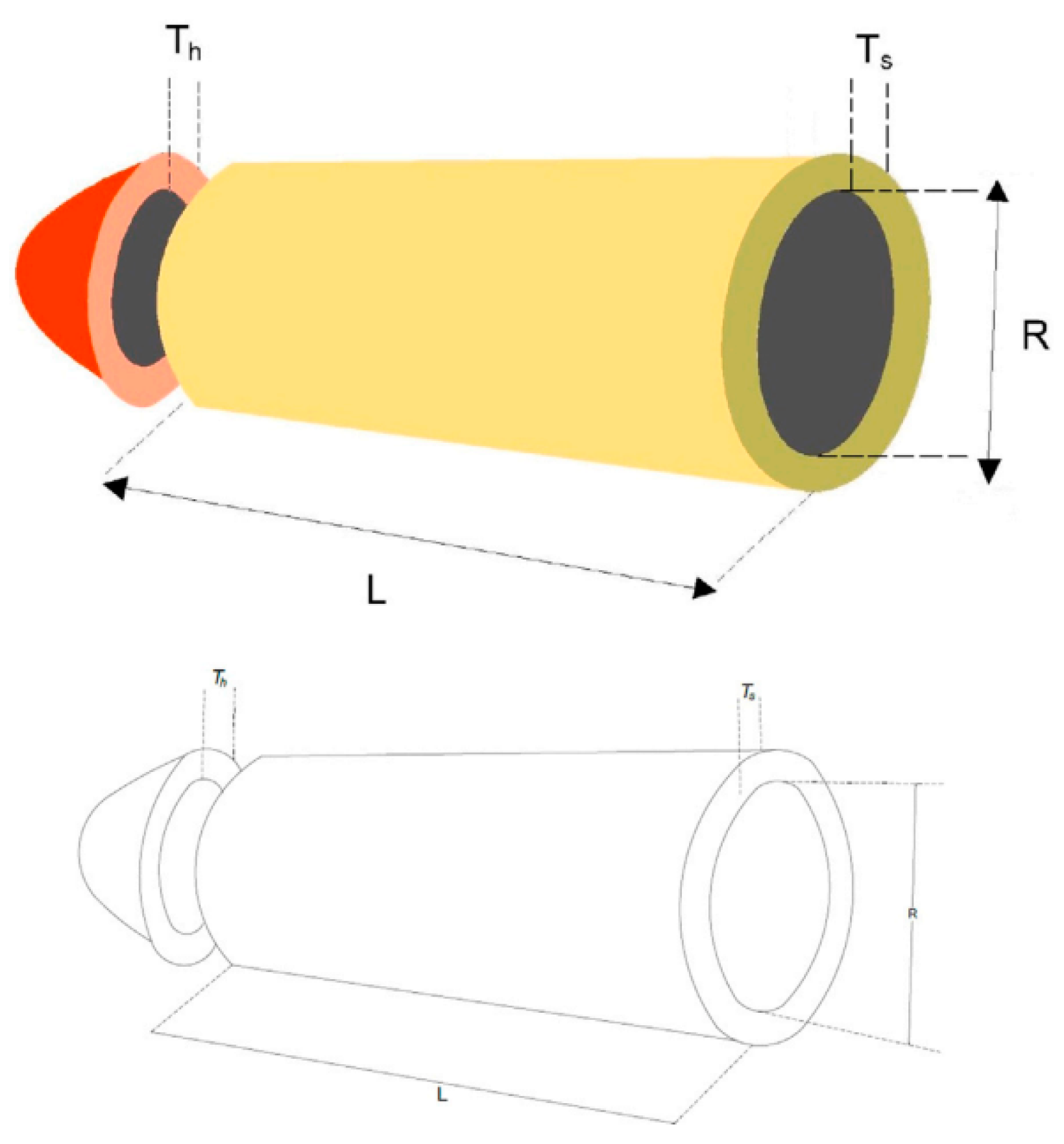
Figure 14.
WBD structure.
Figure 14.
WBD structure.
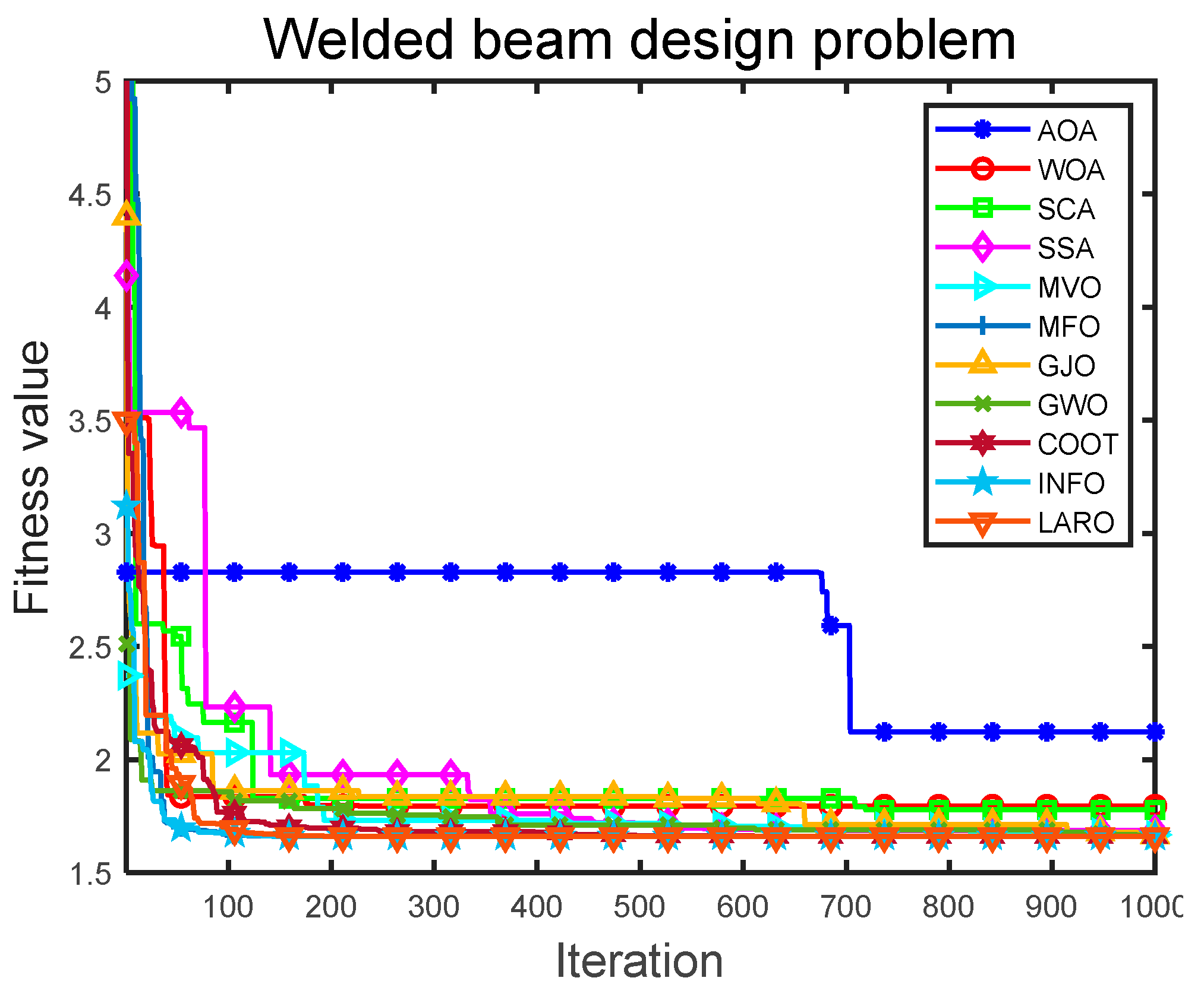
Figure 15.
Convergence iteration plot of LARO and comparison algorithms in WBD problem.
Figure 15.
Convergence iteration plot of LARO and comparison algorithms in WBD problem.
Figure 16.
PVD structure.
Figure 16.
PVD structure.
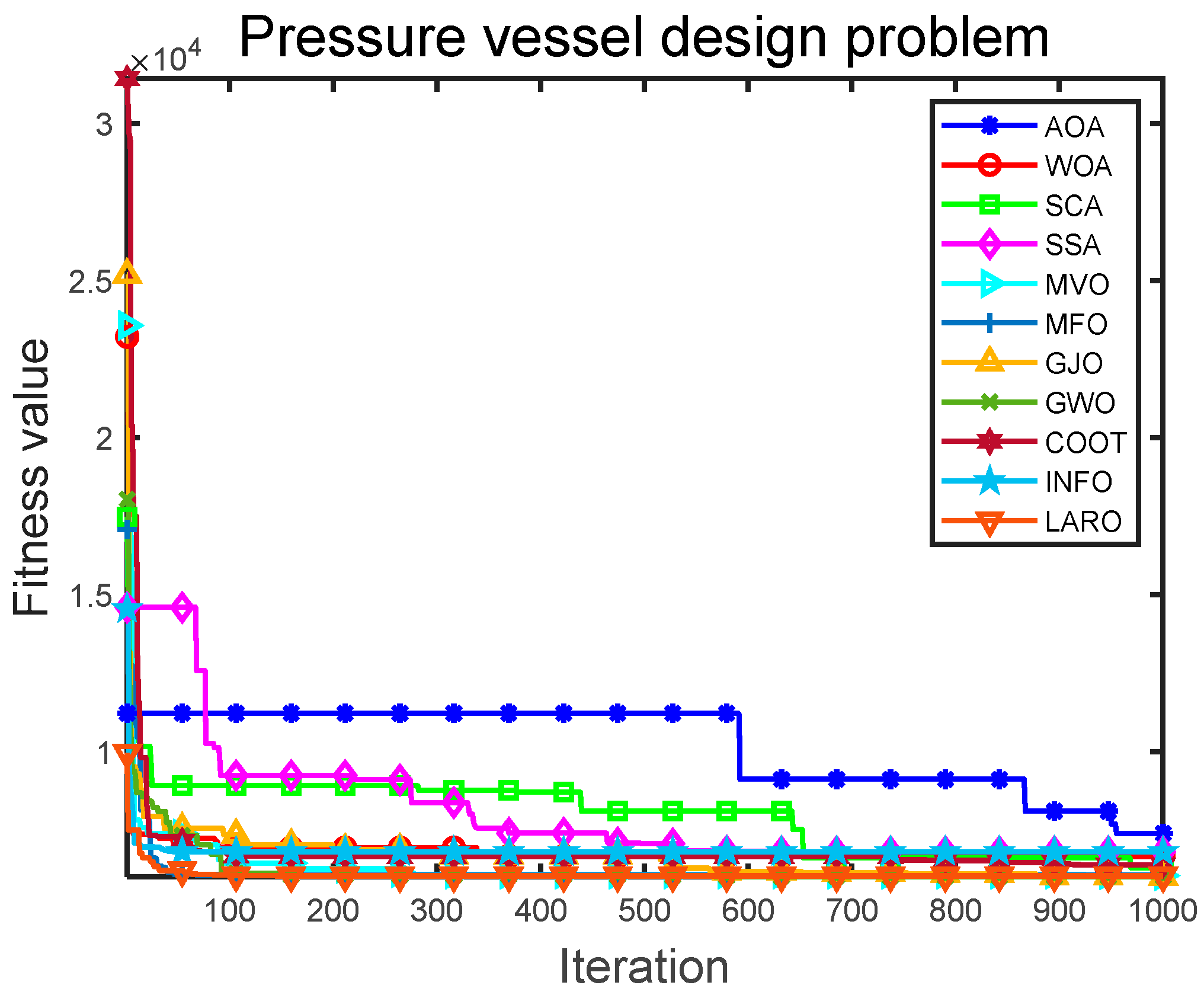
Figure 17.
Convergence iteration plot of LARO and comparison algorithms in PVD problem.
Figure 17.
Convergence iteration plot of LARO and comparison algorithms in PVD problem.
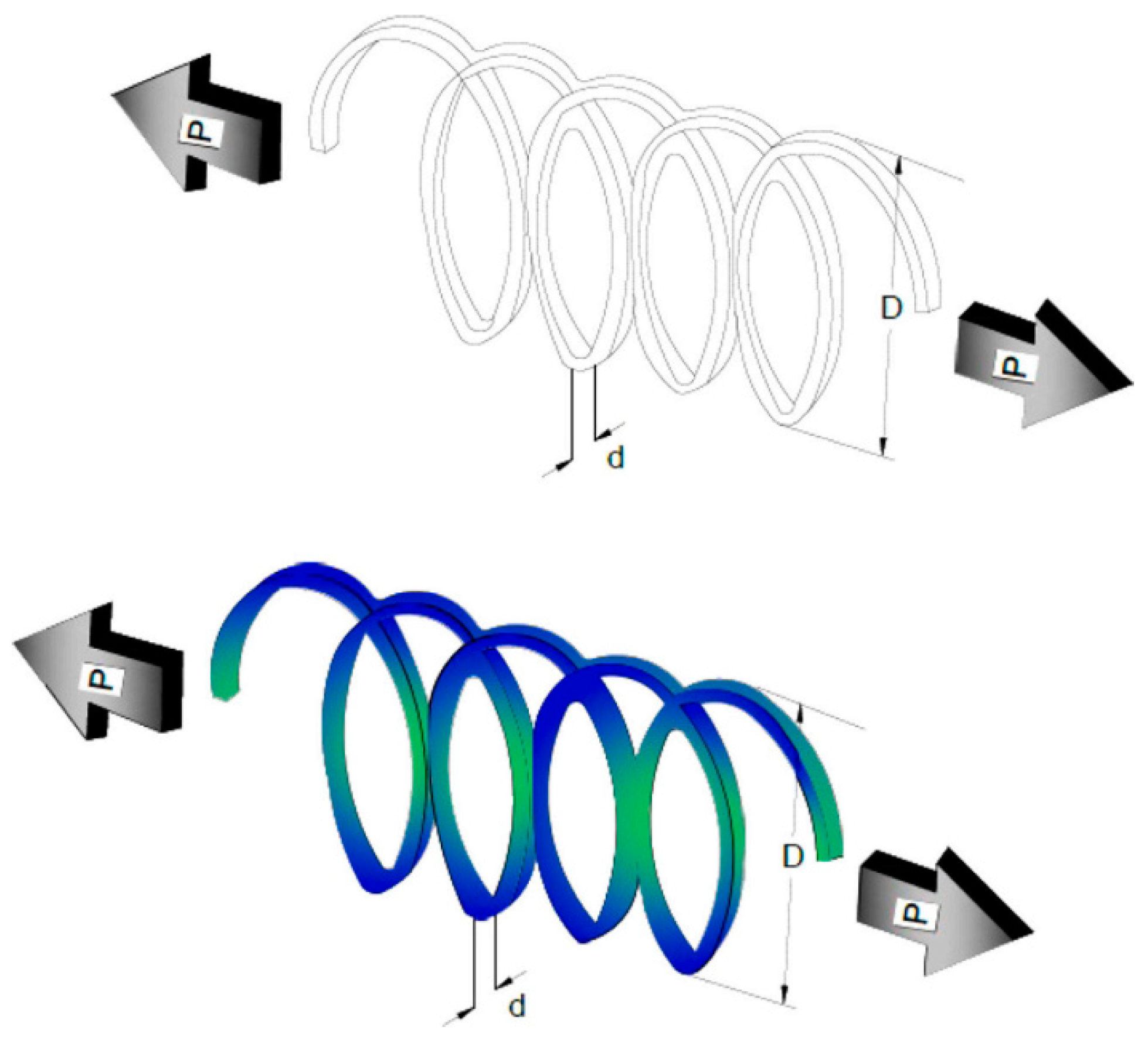
Figure 18.
TCS structure.
Figure 18.
TCS structure.
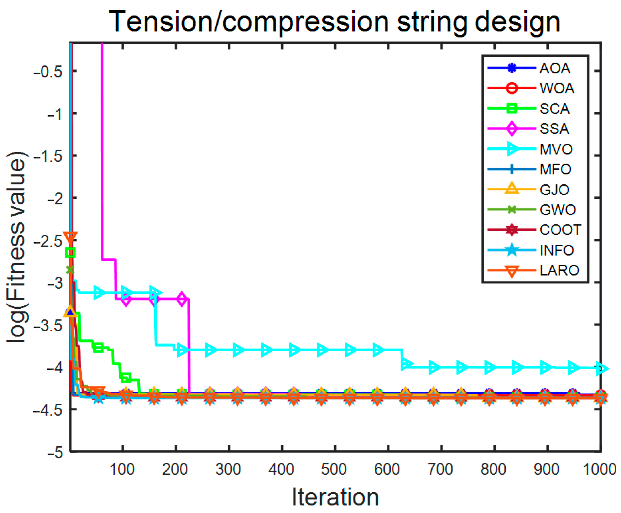
Figure 19.
Convergence iteration plot of LARO and comparison algorithms in TCS problem.
Figure 19.
Convergence iteration plot of LARO and comparison algorithms in TCS problem.
Figure 20.
GTD structure.
Figure 20.
GTD structure.
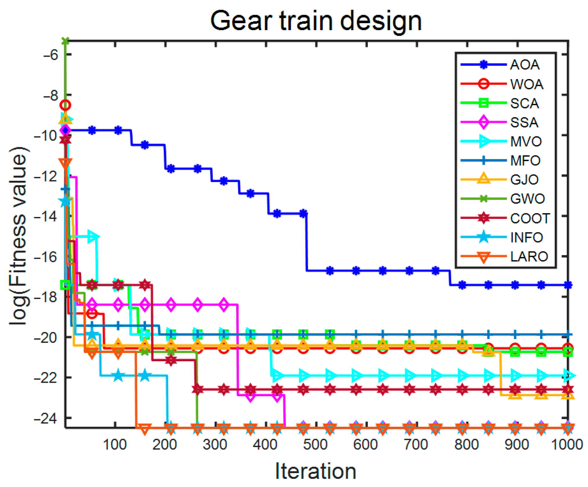
Figure 21.
Convergence iteration plot of LARO and comparison algorithms in GTD problem.
Figure 21.
Convergence iteration plot of LARO and comparison algorithms in GTD problem.
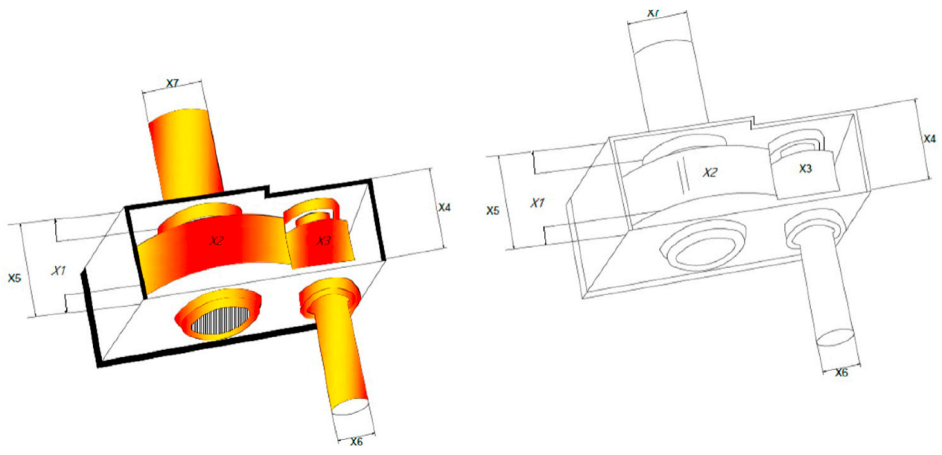
Figure 22.
SRD structure.
Figure 22.
SRD structure.
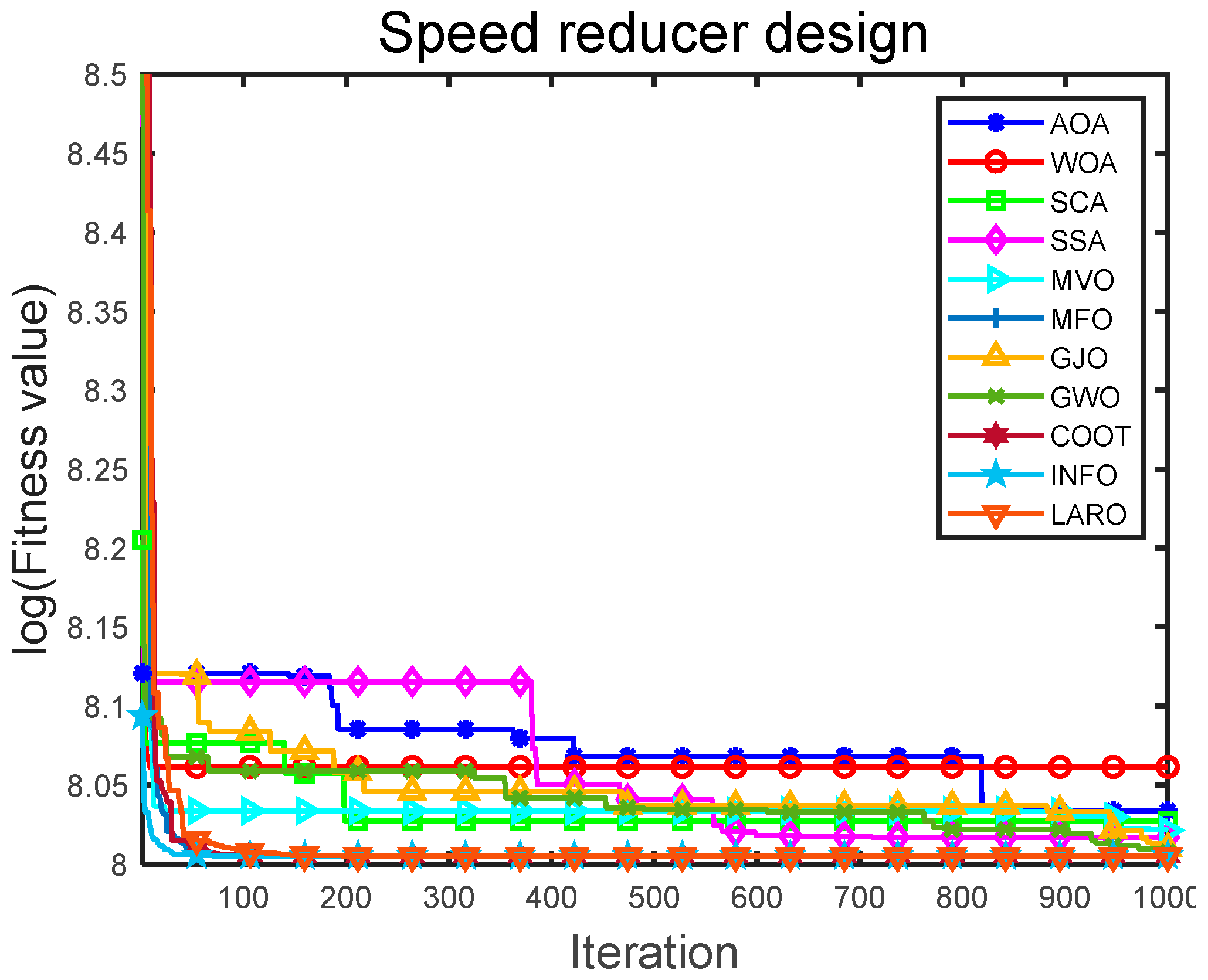
Figure 23.
Convergence iteration plot of LARO and comparison algorithms in SRD problem.
Figure 23.
Convergence iteration plot of LARO and comparison algorithms in SRD problem.
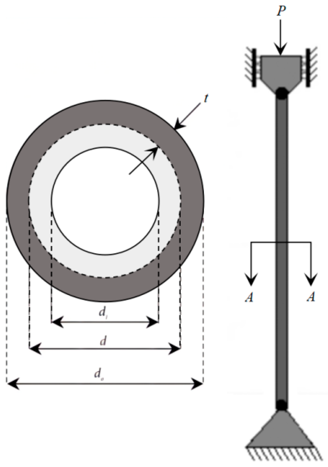
Figure 24.
TCD structure.
Figure 24.
TCD structure.
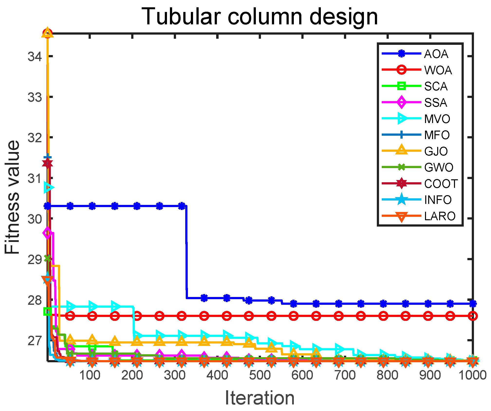
Figure 25.
Convergence iteration plot of LARO and comparison algorithms in TCD problem.
Figure 25.
Convergence iteration plot of LARO and comparison algorithms in TCD problem.
Table 1.
Suitable parameters for different algorithms.
Table 1.
Suitable parameters for different algorithms.
| Methods | Parameters | Value Situation |
|---|
| AOA [38] | µ | 0.499 |
| | a | a5 |
| GWO [39] | Convergence parameter (a) | Linear decrease from 2 to 0 |
| WOA [47] | A | Drop from 2 to 0 |
| | b | 2 |
| SSA [46] | Leader position update probability | c3 = 0.5 |
| INFO [42] | c | 2 |
| | d | 4 |
| MVO [43] | Wormhole Existence Probability WEPMax | 1 |
| | Wormhole Existence Probability WEPMin | 0.2 |
| SCA [44] | A | 2 |
Table 2.
Comparison of LARO with two different parameters in 23 benchmark functions.
Table 2.
Comparison of LARO with two different parameters in 23 benchmark functions.
| Functions | Algorithms | Mean | STD | Time | Functions | Algorithms | Mean | STD | Time |
|---|
| F01 | LARO1 | 2.17E-181 | 0 | 7.22299 | F13 | LARO1 | 0.00110 | 0.00338 | 22.00742 |
| LARO2 | 4.78E-91 | 1.39E-90 | 7.38622 | LARO2 | 0.00059 | 0.00247 | 19.16593 |
| F02 | LARO1 | 1.45E-96 | 6.15E-96 | 6.97114 | F14 | LARO1 | 0.99800 | 0 | 31.32199 |
| LARO2 | 1.90E-49 | 3.98E-49 | 6.97564 | LARO2 | 0.99800 | 0 | 29.23997 |
| F03 | LARO1 | 5.18E-146 | 1.97E-145 | 16.08589 | F15 | LARO1 | 0.00031 | 2.97E-16 | 5.84512 |
| LARO2 | 5.48E-73 | 2.11E-72 | 14.75086 | LARO2 | 0.00031 | 2.37E-08 | 6.53547 |
| F04 | LARO1 | 8.57E-75 | 3.61E-74 | 7.35237 | F16 | LARO1 | −1.03163 | 2.16E-16 | 5.51881 |
| LARO2 | 1.10E-37 | 2.49E-37 | 6.88073 | LARO2 | −1.03163 | 2.10E-16 | 6.22799 |
| F05 | LARO1 | 0.00470 | 0.00436 | 7.95983 | F17 | LARO1 | 0.39789 | 0 | 5.33003 |
| LARO2 | 0.03234 | 0.03371 | 7.86360 | LARO2 | 0.39789 | 0 | 6.17085 |
| F06 | LARO1 | 5.06E-06 | 6.23E-06 | 6.85314 | F18 | LARO1 | 3 | 5.94E-16 | 5.36706 |
| LARO2 | 0.00014 | 0.00012 | 6.81894 | LARO2 | 3 | 6.28E-16 | 5.99102 |
| F07 | LARO1 | 0.00021 | 0.00014 | 10.94454 | F19 | LARO1 | −3.86278 | 2.28E-15 | 6.59347 |
| LARO2 | 0.00032 | 0.00021 | 10.75831 | LARO2 | −3.86278 | 2.28E-15 | 6.07269 |
| F08 | LARO1 | −1.15E+04 | 334.44374 | 8.30804 | F20 | LARO1 | −3.29227 | 0.05282 | 6.68436 |
| LARO2 | −1.15E+04 | 299.32023 | 8.43271 | LARO2 | −3.32200 | 4.44E-16 | 7.05183 |
| F09 | LARO1 | 0 | 0 | 7.25003 | F21 | LARO1 | −10.15320 | 3.36E-15 | 11.62110 |
| LARO2 | 0 | 0 | 7.61304 | LARO2 | −10.15320 | 2.79E-15 | 7.59196 |
| F10 | LARO1 | 8.88E-16 | 0 | 8.25929 | F22 | LARO1 | −10.06901 | 1.49339 | 9.18435 |
| LARO2 | 8.88E-16 | 0 | 7.80431 | LARO2 | −10.40294 | 3.58E-15 | 8.20396 |
| F11 | LARO1 | 0 | 0 | 8.49955 | F23 | LARO1 | −10.53636 | 0.00024 | 8.69545 |
| LARO2 | 0 | 0 | 8.82418 | LARO2 | −10.53641 | 1.58E-15 | 9.09290 |
| F12 | LARO1 | 2.43E-07 | 2.89E-07 | 20.03895 | | | | | |
| LARO2 | 6.01E-06 | 2.89E-06 | 20.26232 | | | | | |
Table 3.
Performance analysis of jump parameter α in CEC2019.
Table 3.
Performance analysis of jump parameter α in CEC2019.
| Function | Index | Algorithms |
|---|
| α = 0.1 | α = 0.01 | α = 0.05 | α = 0.5 | α = [0.01, 0.05] | α = [0.05, 0.1] | α = [0.1, 0.5] |
|---|
| cec01 | Mean | 1 | 1 | 1 | 1 | 1 | 1 | 1 |
| Rank | 1 | 1 | 1 | 1 | 1 | 1 | 1 |
| cec02 | Mean | 4.2462 | 4.2195 | 4.2553 | 4.2226 | 4.1176 | 4.2233 | 4.2304 |
| Rank | 6 | 2 | 7 | 3 | 1 | 4 | 5 |
| cec03 | Mean | 1.7488 | 1.5887 | 1.5539 | 1.5272 | 1.6122 | 1.7864 | 1.6667 |
| Rank | 6 | 3 | 2 | 1 | 4 | 7 | 5 |
| cec04 | Mean | 12.8513 | 11.0993 | 12.6871 | 16.1851 | 13.7460 | 13.8487 | 13.8736 |
| Rank | 3 | 1 | 2 | 7 | 4 | 5 | 6 |
| cec05 | Mean | 1.0747 | 1.1089 | 1.1029 | 1.0880 | 1.0876 | 1.0790 | 1.0776 |
| Rank | 1 | 7 | 6 | 5 | 4 | 3 | 2 |
| cec06 | Mean | 1.5055 | 1.5995 | 1.6011 | 1.4881 | 1.4857 | 1.4156 | 1.4059 |
| Rank | 5 | 6 | 7 | 4 | 3 | 2 | 1 |
| cec07 | Mean | 386.6686 | 437.5734 | 464.3752 | 450.1384 | 467.1603 | 489.9973 | 465.0378 |
| Rank | 1 | 2 | 4 | 3 | 6 | 7 | 5 |
| cec08 | Mean | 3.0415 | 3.3443 | 3.0979 | 3.2720 | 3.2620 | 3.4022 | 3.5178 |
| Rank | 1 | 5 | 2 | 4 | 3 | 6 | 7 |
| cec09 | Mean | 1.1386 | 1.1156 | 1.1255 | 1.1151 | 1.1143 | 1.1186 | 1.1130 |
| Rank | 7 | 4 | 6 | 3 | 2 | 5 | 1 |
| cec10 | Mean | 18.0553 | 20.0059 | 19.9964 | 20.0029 | 20.0859 | 21.0005 | 20.0014 |
| Rank | 1 | 5 | 2 | 4 | 6 | 7 | 3 |
| Mean rank | 3.2 | 3.6 | 3.9 | 3.5 | 3.4 | 4.7 | 3.6 |
| Final ranking | 1 | 4 | 6 | 3 | 2 | 7 | 4 |
Table 4.
Statistical outcomes of the different MH methods on the 23 test functions.
Table 4.
Statistical outcomes of the different MH methods on the 23 test functions.
| Function | Index | Algorithms |
|---|
| ARO | AOA | GWO | COOT | GJO | INFO | MFO | MVO | SCA | SSA | WOA | LARO |
|---|
| F1 | Best | 1.21E-138 | 9.28E-10 | 5.04E-73 | 1.68E-93 | 7.76E-132 | 9.34E-56 | 1.60E-06 | 0.0009 | 2.20E-07 | 5.37E-09 | 1.09E-186 | 6.69E-199 |
| Worst | 2.30E-127 | 9.90E-07 | 2.39E-69 | 2.23E-18 | 9.04E-127 | 4.43E-55 | 1.00E+04 | 0.0049 | 0.0073 | 1.10E-08 | 6.38E-173 | 2.12E-177 |
| Mean | 1.74E-128 | 4.73E-07 | 3.70E-70 | 1.12E-19 | 9.55E-128 | 3.11E-55 | 1.00E+03 | 0.0023 | 0.0010 | 8.60E-09 | 4.09E-174 | 1.08E-178 |
| STD | 5.61E-128 | 2.34E-07 | 7.22E-70 | 4.99E-19 | 2.29E-127 | 9.13E-56 | 3.08E+03 | 0.0009 | 0.0019 | 1.60E-09 | 0 | 0 |
| Rank | 3 | 9 | 5 | 7 | 4 | 6 | 12 | 11 | 10 | 8 | 2 | 1 |
| F2 | Best | 1.06E-74 | 2.49E-13 | 4.85E-42 | 1.57E-47 | 1.47E-143 | 7.02E-29 | 2.94E-20 | 0.0054 | 2.91E-24 | 4.52E-06 | 7.23E-118 | 4.88E-105 |
| Worst | 2.80E-67 | 0.0006 | 1.55E-40 | 7.37E-18 | 8.09E-137 | 2.40E-28 | 1.43E-18 | 0.0216 | 3.94E-20 | 8.69E-06 | 4.13E-105 | 1.84E-95 |
| Mean | 2.19E-68 | 0.0001 | 3.81E-41 | 3.68E-19 | 6.36E-138 | 1.58E-28 | 2.79E-19 | 0.0130 | 3.20E-21 | 6.09E-06 | 2.10E-106 | 9.20E-97 |
| STD | 6.66E-68 | 0.0002 | 4.24E-41 | 1.65E-18 | 1.82E-137 | 3.66E-29 | 3.93E-19 | 0.0039 | 9.22E-21 | 1.28E-06 | 9.22E-106 | 4.11E-96 |
| Rank | 4 | 11 | 5 | 9 | 1 | 6 | 8 | 12 | 7 | 10 | 2 | 3 |
| F3 | Best | 2.19E-115 | 7.27E-08 | 9.95E-24 | 1.69E-108 | 5.66E-150 | 1.41E-55 | 7.16E-12 | 0.0024 | 2.53E-20 | 4.86E-10 | 1.02E+03 | 9.25E-160 |
| Worst | 4.64E-98 | 0.0005 | 1.70E-18 | 3.75E-17 | 3.30E-136 | 3.43E-54 | 7.83E-08 | 0.0274 | 4.50E-09 | 2.26E-09 | 2.52E+04 | 8.97E-145 |
| Mean | 2.99E-99 | 0.0001 | 1.35E-19 | 1.87E-18 | 2.21E-137 | 7.44E-55 | 6.93E-09 | 0.0152 | 2.35E-10 | 1.31E-09 | 9.94E+03 | 6.05E-146 |
| STD | 1.06E-98 | 0.0001 | 4.11E-19 | 8.38E-18 | 7.66E-137 | 7.17E-55 | 1.99E-08 | 0.0085 | 1.00E-09 | 5.18E-10 | 7.06E+03 | 2.09E-145 |
| Rank | 3 | 10 | 5 | 6 | 2 | 4 | 9 | 11 | 7 | 8 | 12 | 1 |
| F4 | Best | 2.49E-59 | 0.0012 | 8.10E-19 | 1.00E-50 | 3.15E-102 | 3.80E-29 | 2.24E-10 | 0.0149 | 8.01E-14 | 9.04E-06 | 2.09E-05 | 6.58E-83 |
| Worst | 1.51E-51 | 0.0386 | 8.67E-17 | 1.10E-18 | 2.48E-94 | 9.71E-29 | 4.81E-06 | 0.0558 | 3.26E-09 | 1.97E-05 | 83.8975 | 1.08E-74 |
| Mean | 8.18E-53 | 0.0082 | 9.98E-18 | 5.69E-20 | 1.34E-95 | 7.06E-29 | 3.41E-07 | 0.0289 | 5.72E-10 | 1.49E-05 | 26.7587 | 5.69E-76 |
| STD | 3.36E-52 | 0.0095 | 1.86E-17 | 2.46E-19 | 5.54E-95 | 1.69E-29 | 1.09E-06 | 0.0109 | 1.01E-09 | 2.60E-06 | 27.7544 | 2.40E-75 |
| Rank | 3 | 10 | 6 | 5 | 1 | 4 | 8 | 11 | 7 | 9 | 12 | 2 |
| F5 | Best | 0.0006 | 26.3419 | 25.1729 | 12.7342 | 5.9635 | 1.00E-15 | 0.5337 | 0.3466 | 6.3912 | 1.0423 | 25.9605 | 0.0002 |
| Worst | 0.0090 | 27.8627 | 27.9110 | 164.4579 | 8.7006 | 3.82E-08 | 9.00E+04 | 420.5066 | 8.0566 | 326.6321 | 26.9912 | 0.0259 |
| Mean | 0.0029 | 26.9276 | 26.6522 | 33.4068 | 6.8759 | 4.47E-09 | 4.68E+03 | 43.9598 | 7.0330 | 48.0257 | 26.5465 | 0.0057 |
| STD | 0.0023 | 0.3875 | 0.6903 | 31.0189 | 0.7159 | 1.08E-08 | 2.01E+04 | 100.2646 | 0.3919 | 81.8641 | 0.3124 | 0.0069 |
| Rank | 2 | 8 | 7 | 9 | 4 | 1 | 12 | 10 | 5 | 11 | 6 | 3 |
| F6 | Best | 2.65E-07 | 0.3379 | 8.71E-06 | 3.83E-05 | 1.56E-06 | 0 | 0 | 0.0011 | 0.1184 | 2.99E-10 | 0.0017 | 8.78E-07 |
| Worst | 2.57E-06 | 0.8442 | 0.9951 | 0.0009 | 0.4997 | 4.93E-32 | 4.50E-31 | 0.0039 | 0.5995 | 9.36E-10 | 0.0073 | 1.50E-05 |
| Mean | 1.09E-06 | 0.5939 | 0.2872 | 0.0003 | 0.1376 | 6.16E-33 | 6.39E-32 | 0.0023 | 0.2553 | 6.36E-10 | 0.0041 | 4.77E-06 |
| STD | 6.58E-07 | 0.1378 | 0.2839 | 0.0002 | 0.1512 | 1.16E-32 | 1.13E-31 | 0.0008 | 0.1261 | 1.80E-10 | 0.0015 | 4.17E-06 |
| Rank | 4 | 12 | 11 | 6 | 9 | 1 | 2 | 7 | 10 | 3 | 8 | 5 |
| F7 | Best | 2.92E-05 | 3.42E-08 | 0.0001 | 0.0001 | 6.24E-06 | 7.13E-05 | 0.0005 | 0.0002 | 0.0001 | 0.0005 | 2.56E-05 | 1.02E-05 |
| Worst | 0.0006 | 6.65E-05 | 0.0013 | 0.0090 | 0.0002 | 0.0013 | 0.0066 | 0.0035 | 0.0024 | 0.0118 | 0.0025 | 0.0004 |
| Mean | 0.0002 | 2.38E-05 | 0.0005 | 0.0021 | 6.19E-05 | 0.0003 | 0.0026 | 0.0012 | 0.0006 | 0.0045 | 0.0006 | 0.0002 |
| STD | 0.0002 | 2.11E-05 | 0.0003 | 0.0023 | 5.14E-05 | 0.0003 | 0.0014 | 0.0008 | 0.0006 | 0.0031 | 0.0006 | 0.0001 |
| Rank | 4 | 1 | 6 | 10 | 2 | 5 | 11 | 9 | 8 | 12 | 7 | 3 |
| F8 | Best | −1.18E+04 | −6.15E+03 | −7.74E+03 | −8.96E+03 | −2.77E+03 | −4.19E+03 | −4.19E+03 | −3.83E+03 | −2.64E+03 | −3.30E+03 | −1.26E+04 | −1.21E+04 |
| Worst | −1.02E+04 | −4.95E+03 | −4.93E+03 | −7.04E+03 | −1.84E+03 | −3.36E+03 | −2.52E+03 | −2.43E+03 | −2.05E+03 | −2.23E+03 | −8.37E+03 | −1.08E+04 |
| Mean | −1.09E+04 | −5.49E+03 | −6.35E+03 | −7.90E+03 | −2.32E+03 | −3.63E+03 | −3.38E+03 | −3.16E+03 | −2.30E+03 | −2.80E+03 | −1.20E+04 | −1.16E+04 |
| STD | 4.52E+02 | 3.84E+02 | 7.00E+02 | 5.59E+02 | 2.58E+02 | 2.08E+02 | 3.78E+02 | 3.27E+02 | 1.55E+02 | 2.95E+02 | 1.18E+03 | 3.94E+02 |
| Rank | 3 | 6 | 5 | 4 | 11 | 7 | 8 | 9 | 12 | 10 | 1 | 2 |
| F9 | Best | 0 | 0 | 0 | 0 | 0 | 0 | 3.9798 | 3.9804 | 0 | 6.9647 | 0 | 0 |
| Worst | 0 | 4.39E-07 | 11.5726 | 1.71E-13 | 0 | 0 | 44.8440 | 22.8853 | 0.3257 | 41.7882 | 5.68E-14 | 0 |
| Mean | 0 | 1.10E-07 | 1.0975 | 8.53E-15 | 0 | 0 | 17.9128 | 12.0401 | 0.0163 | 15.0239 | 2.84E-15 | 0 |
| STD | 0 | 1.55E-07 | 2.9474 | 3.81E-14 | 0 | 0 | 10.3395 | 5.8096 | 0.0728 | 7.9590 | 1.27E-14 | 0 |
| Rank | 1 | 7 | 9 | 6 | 1 | 1 | 12 | 10 | 8 | 11 | 5 | 1 |
| F10 | Best | 8.88E-16 | 7.48E-08 | 7.99E-15 | 8.88E-16 | 8.88E-16 | 8.88E-16 | 4.44E-15 | 0.0088 | 8.88E-16 | 5.88E-06 | 8.88E-16 | 8.88E-16 |
| Worst | 8.88E-16 | 0.0003 | 1.87E-14 | 1.54E-11 | 4.44E-15 | 8.88E-16 | 7.99E-15 | 0.0228 | 7.99E-15 | 2.0133 | 7.99E-15 | 8.88E-16 |
| Mean | 8.88E-16 | 0.0001 | 1.40E-14 | 8.04E-13 | 3.91E-15 | 8.88E-16 | 4.62E-15 | 0.0178 | 4.80E-15 | 0.5489 | 4.09E-15 | 8.88E-16 |
| STD | 0 | 8.13E-05 | 2.33E-15 | 3.43E-12 | 1.30E-15 | 0 | 7.94E-16 | 0.0035 | 1.59E-15 | 0.8664 | 2.28E-15 | 0 |
| Rank | 1 | 10 | 8 | 9 | 4 | 1 | 6 | 11 | 7 | 12 | 5 | 1 |
| F11 | Best | 0 | 1.15E-06 | 0 | 0 | 0 | 0 | 0.0271 | 0.1110 | 0 | 0.0836 | 0 | 0 |
| Worst | 0 | 0.0123 | 0.0404 | 2.22E-16 | 0 | 0 | 0.3173 | 0.5909 | 0.7448 | 0.7018 | 0.0372 | 0 |
| Mean | 0 | 0.0006 | 0.0027 | 1.11E-17 | 0 | 0 | 0.1347 | 0.3030 | 0.0381 | 0.2650 | 0.0034 | 0 |
| STD | 0 | 0.0028 | 0.0094 | 4.97E-17 | 0 | 0 | 0.0818 | 0.1209 | 0.1664 | 0.1495 | 0.0104 | 0 |
| Rank | 1 | 6 | 7 | 5 | 1 | 1 | 10 | 12 | 9 | 11 | 8 | 1 |
| F12 | Best | 1.11E-08 | 0.4017 | 0.0054 | 7.28E-07 | 8.14E-07 | 4.71E-32 | 4.71E-32 | 2.93E-05 | 0.0300 | 3.35E-12 | 0.0001 | 3.24E-08 |
| Worst | 2.49E-07 | 0.5290 | 0.0581 | 0.1037 | 0.0593 | 4.93E-32 | 0.9329 | 0.3122 | 0.1082 | 0.3712 | 0.0201 | 1.16E-06 |
| Mean | 6.05E-08 | 0.4541 | 0.0253 | 0.0052 | 0.0298 | 4.79E-32 | 0.1088 | 0.0313 | 0.0655 | 0.0688 | 0.0016 | 3.27E-07 |
| STD | 5.65E-08 | 0.0331 | 0.0158 | 0.0232 | 0.0218 | 8.02E-34 | 0.2527 | 0.0960 | 0.0205 | 0.1336 | 0.0044 | 3.40E-07 |
| Rank | 2 | 12 | 6 | 5 | 7 | 1 | 11 | 8 | 9 | 10 | 4 | 3 |
| F13 | Best | 7.63E-08 | 2.8252 | 1.91E-05 | 7.71E-05 | 3.30E-06 | 1.35E-32 | 1.35E-32 | 0.0001 | 0.0798 | 1.39E-11 | 0.0027 | 1.95E-07 |
| Worst | 0.0439 | 2.9661 | 0.4064 | 0.0364 | 0.3992 | 0.0439 | 0.0110 | 0.0118 | 0.3257 | 0.0110 | 0.1943 | 7.23E-06 |
| Mean | 0.0039 | 2.9528 | 0.2462 | 0.0091 | 0.1081 | 0.0033 | 0.0016 | 0.0015 | 0.2240 | 0.0016 | 0.0522 | 1.81E-06 |
| STD | 0.0102 | 0.0408 | 0.1180 | 0.0092 | 0.1023 | 0.0101 | 0.0040 | 0.0034 | 0.0648 | 0.0040 | 0.0605 | 1.90E-06 |
| Rank | 6 | 12 | 11 | 7 | 9 | 5 | 3 | 2 | 10 | 4 | 8 | 1 |
| F14 | Best | 0.9980 | 0.9980 | 0.9980 | 0.9980 | 0.9980 | 0.9980 | 0.9980 | 0.9980 | 0.9980 | 0.9980 | 0.9980 | 0.9980 |
| Worst | 0.9980 | 12.6705 | 12.6705 | 0.9980 | 12.6705 | 2.9821 | 1.9920 | 0.9980 | 2.9821 | 0.9980 | 10.7632 | 0.9980 |
| Mean | 0.9980 | 8.4157 | 5.2933 | 0.9980 | 4.9158 | 1.1469 | 1.0974 | 0.9980 | 1.4941 | 0.9980 | 2.6117 | 0.9980 |
| STD | 0 | 4.4965 | 5.0354 | 2.88E-16 | 4.2395 | 0.4857 | 0.3060 | 5.24E-12 | 0.8814 | 1.02E-16 | 3.5461 | 0 |
| Rank | 1 | 12 | 11 | 1 | 10 | 7 | 6 | 5 | 8 | 1 | 9 | 1 |
| F15 | Best | 0.0003 | 0.0003 | 0.0003 | 0.0003 | 0.0003 | 0.0003 | 0.0006 | 0.0003 | 0.0004 | 0.0003 | 0.0003 | 0.0003 |
| Worst | 0.0003 | 0.0207 | 0.0204 | 0.0012 | 0.0012 | 0.0012 | 0.0023 | 0.0204 | 0.0015 | 0.0012 | 0.0014 | 0.0003 |
| Mean | 0.0003 | 0.0031 | 0.0024 | 0.0004 | 0.0004 | 0.0004 | 0.0010 | 0.0066 | 0.0009 | 0.0007 | 0.0006 | 0.0003 |
| STD | 2.47E-19 | 0.0051 | 0.0062 | 0.0002 | 0.0003 | 0.0002 | 0.0004 | 0.0093 | 0.0004 | 0.0003 | 0.0003 | 1.29E-16 |
| Rank | 1 | 11 | 10 | 4 | 5 | 3 | 9 | 12 | 8 | 7 | 6 | 2 |
| F16 | Best | −1.0316 | −1.0316 | −1.0316 | −1.0316 | −1.0316 | −1.0316 | −1.0316 | −1.0316 | −1.0316 | −1.0316 | −1.0316 | −1.0316 |
| Worst | −1.0316 | −1.0316 | −1.0316 | −1.0316 | −1.0316 | −1.0316 | −1.0316 | −1.0316 | −1.0316 | −1.0316 | −1.0316 | −1.0316 |
| Mean | −1.0316 | −1.0316 | −1.0316 | −1.0316 | −1.0316 | −1.0316 | −1.0316 | −1.0316 | −1.0316 | −1.0316 | −1.0316 | −1.0316 |
| STD | 2.22E-16 | 7.42E-12 | 3.08E-09 | 4.04E-14 | 1.70E-08 | 2.28E-16 | 2.28E-16 | 6.22E-08 | 1.79E-05 | 6.02E-15 | 1.97E-11 | 2.28E-16 |
| Rank | 1 | 8 | 9 | 5 | 10 | 1 | 1 | 11 | 12 | 5 | 7 | 1 |
| F17 | Best | 0.3979 | 0.4960 | 0.3979 | 0.3979 | 0.3979 | 0.3979 | 0.3979 | 0.3979 | 0.3979 | 0.3979 | 0.3979 | 0.3979 |
| Worst | 0.3979 | 2.5958 | 0.3979 | 0.3979 | 0.3981 | 0.3979 | 0.3979 | 0.3979 | 0.3994 | 0.3979 | 0.3979 | 0.3979 |
| Mean | 0.3979 | 1.3108 | 0.3979 | 0.3979 | 0.3979 | 0.3979 | 0.3979 | 0.3979 | 0.3984 | 0.3979 | 0.3979 | 0.3979 |
| STD | 0 | 0.6557 | 4.30E-07 | 7.30E-08 | 3.92E-05 | 0 | 0 | 7.31E-08 | 0.0004 | 4.68E-15 | 8.28E-08 | 0 |
| Rank | 1 | 12 | 9 | 6 | 10 | 1 | 1 | 8 | 11 | 5 | 7 | 1 |
| F18 | Best | 3 | 3 | 3.0000 | 3 | 3.0000 | 3 | 3 | 3.0000 | 3.0000 | 3 | 3.0000 | 3 |
| Worst | 3 | 30 | 3.0000 | 3 | 3.0000 | 3 | 3 | 3.0000 | 3.0000 | 3 | 3.0000 | 3 |
| Mean | 3 | 11.1 | 3.0000 | 3 | 3.0000 | 3 | 3 | 3.0000 | 3.0000 | 3 | 3.0000 | 3 |
| STD | 6.28E-16 | 12.6944 | 4.15E-06 | 2.78E-14 | 4.45E-07 | 2.88E-16 | 1.45E-15 | 3.93E-07 | 9.62E-06 | 4.37E-14 | 4.46E-06 | 9.56E-16 |
| Rank | 1 | 12 | 10 | 5 | 7 | 1 | 1 | 8 | 11 | 6 | 9 | 1 |
| F19 | Best | −3.8628 | −3.8628 | −3.8628 | −3.8628 | −3.8628 | −3.8628 | −3.8628 | −3.8628 | −3.8623 | −3.8628 | −3.8628 | −3.8628 |
| Worst | −3.8628 | −3.8628 | −3.8549 | −3.8628 | −3.8549 | −3.8628 | −3.8628 | −3.8628 | −3.8535 | −3.8628 | −3.8549 | −3.8628 |
| Mean | −3.8628 | −3.8628 | −3.8615 | −3.8628 | −3.8592 | −3.8628 | −3.8628 | −3.8628 | −3.8569 | −3.8628 | −3.8614 | −3.8628 |
| STD | 2.28E-15 | 6.30E-07 | 0.0028 | 2.03E-15 | 0.0040 | 2.28E-15 | 2.28E-15 | 1.34E-07 | 0.0034 | 1.51E-14 | 0.0028 | 2.28E-15 |
| Rank | 1 | 8 | 9 | 1 | 11 | 1 | 1 | 7 | 12 | 6 | 10 | 1 |
| F20 | Best | −3.3220 | −3.3220 | −3.3220 | −3.3220 | −3.3220 | −3.3220 | −3.3220 | −3.3220 | −3.1559 | −3.3220 | −3.3220 | −3.3220 |
| Worst | −3.2031 | −3.2031 | −3.1981 | −3.2031 | −2.8404 | −3.2031 | −3.1376 | −3.2024 | −2.6213 | −3.1989 | −3.0867 | −3.2031 |
| Mean | −3.2982 | −3.2804 | −3.2739 | −3.2982 | −3.1169 | −3.2625 | −3.2322 | −3.2565 | −3.0157 | −3.2261 | −3.2356 | −3.3101 |
| STD | 0.0488 | 0.0582 | 0.0605 | 0.0488 | 0.1234 | 0.0610 | 0.0634 | 0.0608 | 0.1298 | 0.0492 | 0.0768 | 0.0366 |
| Rank | 2 | 4 | 5 | 3 | 11 | 6 | 9 | 7 | 12 | 10 | 8 | 1 |
| F21 | Best | −10.1532 | −10.1532 | −10.1531 | −10.1532 | −10.1524 | −10.1532 | −10.1532 | −10.1532 | −6.1684 | −10.1532 | −10.1532 | −10.1532 |
| Worst | −2.6305 | −5.1007 | −5.0552 | −10.1532 | −5.0551 | −2.6305 | −2.6305 | −5.1007 | −0.8798 | −2.6305 | −2.6303 | −10.1532 |
| Mean | −9.7771 | −7.8795 | −9.3905 | −10.1532 | −9.3888 | −9.7771 | −7.3843 | −8.8900 | −3.9983 | −8.7666 | −8.6480 | −10.1532 |
| STD | 1.6821 | 2.5788 | 1.8621 | 3.40E-13 | 1.8613 | 1.6821 | 3.2457 | 2.2446 | 1.7187 | 2.5157 | 3.0870 | 3.51E-15 |
| Rank | 3 | 10 | 5 | 2 | 6 | 3 | 11 | 7 | 12 | 8 | 9 | 1 |
| F22 | Best | −10.4029 | −10.4029 | −10.4029 | −10.4029 | −10.4025 | −10.4029 | −10.4029 | −10.4029 | −7.6292 | −10.4029 | −10.4029 | −10.4029 |
| Worst | −3.7243 | −3.7243 | −10.4021 | −10.4029 | −4.4596 | −2.7659 | −2.7659 | −2.7659 | −0.9097 | −2.7519 | −5.0877 | −10.4017 |
| Mean | −10.0690 | −9.2076 | −10.4026 | −10.4029 | −10.1033 | −8.9235 | −7.5987 | −9.3755 | −4.2828 | −10.0204 | −9.8710 | −10.4029 |
| STD | 1.4934 | 2.4737 | 0.0002 | 3.97E-13 | 1.3284 | 3.0418 | 3.2662 | 2.5480 | 2.0099 | 1.7108 | 1.6359 | 0.0003 |
| Rank | 5 | 9 | 3 | 1 | 4 | 10 | 11 | 8 | 12 | 6 | 7 | 2 |
| F23 | Best | −10.5364 | −10.5364 | −10.5363 | −10.5364 | −10.5363 | −10.5364 | −10.5364 | −10.5364 | −10.2588 | −10.5364 | −10.5364 | −10.5364 |
| Worst | −10.5364 | −2.4217 | −10.5355 | −10.5364 | −10.5304 | −2.4217 | −2.4217 | −5.1756 | −0.9487 | −2.8711 | −2.4217 | −10.5364 |
| Mean | −10.5364 | −8.7521 | −10.5360 | −10.5364 | −10.5337 | −8.6684 | −8.9409 | −9.4642 | −5.0736 | −9.8851 | −8.1094 | −10.5364 |
| STD | 1.82E-15 | 3.2104 | 0.0002 | 2.30E-13 | 0.0014 | 3.3361 | 2.9057 | 2.2000 | 1.6543 | 2.0392 | 3.4234 | 3.43E-15 |
| Rank | 1 | 9 | 4 | 3 | 5 | 10 | 8 | 7 | 12 | 6 | 11 | 1 |
| Mean rank | 2.3478 | 9.0870 | 7.2174 | 5.1739 | 5.8696 | 3.7391 | 7.3913 | 8.8261 | 9.5217 | 7.7826 | 7.0870 | 1.6957 |
| Final ranking | 2 | 11 | 7 | 4 | 5 | 3 | 8 | 10 | 12 | 9 | 6 | 1 |
| +/=/− | 2/16/5 | 1/1/21 | 0/1/22 | 0/11/12 | 3/2/18 | 3/12/8 | 1/5/17 | 0/1/22 | 0/1/22 | 1/7/15 | 2/3/18 | −/−/− |
Table 5.
Statistical output and associated p-values on 23 test functions.
Table 5.
Statistical output and associated p-values on 23 test functions.
| p-Value | ARO | AOA | GWO | COOT | GJO | INFO | MFO | MVO | SCA | SSA | WOA |
|---|
| F1 | 6.80E-08/− | 6.80E-08/− | 6.80E-08/− | 6.80E-08/− | 6.80E-08/− | 6.80E-08/− | 6.80E-08/− | 6.80E-08/− | 6.80E-08/− | 6.80E-08/− | 1.25E-05/− |
| F2 | 6.80E-08/− | 6.80E-08/− | 6.80E-08/− | 6.80E-08/− | 6.80E-08/+ | 6.79E-08/− | 6.80E-08/− | 6.80E-08/− | 6.80E-08/− | 6.80E-08/− | 6.80E-08/+ |
| F3 | 6.80E-08/− | 6.79E-08/− | 6.79E-08/− | 6.80E-08/− | 2.06E-06/− | 6.80E-08/− | 6.80E-08/− | 6.80E-08/− | 6.80E-08/− | 6.80E-08/− | 6.80E-08/− |
| F4 | 6.80E-08/− | 6.80E-08/− | 6.80E-08/− | 6.80E-08/− | 6.80E-08/+ | 6.80E-08/− | 6.80E-08/− | 6.80E-08/− | 6.80E-08/− | 6.79E-08/− | 6.80E-08/− |
| F5 | 0.3507/= | 6.80E-08/− | 6.80E-08/− | 6.80E-08/− | 6.80E-08/− | 6.80E-08/+ | 6.79E-08/− | 6.80E-08/− | 6.80E-08/− | 6.80E-08/− | 6.80E-08/− |
| F6 | 0.0001/+ | 6.80E-08/− | 4.87E-07/− | 6.80E-08/− | 0.0020/− | 4.85E-08/+ | 6.68E-08/+ | 6.80E-08/− | 6.80E-08/− | 6.80E-08/+ | 6.80E-08/− |
| F7 | 0.9676/= | 4.54E-07/+ | 0.0001/− | 6.67E-06/− | 1.92E-05/+ | 0.2733/= | 6.80E-08/− | 6.01E-07/− | 0.0013/− | 6.80E-08/− | 0.0256/− |
| F8 | 0.0003/− | 6.80E-08/− | 6.80E-08/− | 6.80E-08/− | 6.80E-08/− | 6.74E-08/− | 6.72E-08/− | 6.80E-08/− | 6.80E-08/− | 6.79E-08/− | 0.0002/+ |
| F9 | NaN/= | 9.42E-06/− | 0.0198/− | 0.3421/= | NaN/= | NaN/= | 7.98E-09/− | 8.01E-09/− | 0.3421/= | 7.95E-09/− | 0.3421/+ |
| F10 | NaN/= | 8.01E-09/− | 3.84E-09/− | 9.90E-08/− | 8.64E-08/− | NaN/= | 7.43E-10/− | 8.01E-09/− | 8.30E-09/− | 7.98E-09/− | 2.17E-06/− |
| F11 | NaN/= | 8.01E-09/− | 0.1626/= | 0.3421/= | NaN/= | NaN/= | 8.01E-09/− | 8.01E-09/− | 0.0009/− | 8.01E-09/− | 0.1626/= |
| F12 | 1.81E-05/+ | 6.80E-08/− | 6.80E-08/− | 1.06E-07/− | 1.23E-07/− | 6.13E-08/+ | 0.0012/− | 6.80E-08/− | 6.80E-08/− | 0.0071/− | 6.80E-08/− |
| F13 | 0.8604/= | 6.80E-08/− | 6.80E-08/− | 6.80E-08/− | 2.56E-07/− | 0.0001/− | 0.0002/− | 6.80E-08/− | 6.80E-08/− | 0.0002/− | 6.80E-08/− |
| F14 | NaN/= | 9.32E-08/− | 6.41E-05/− | NaN/= | 2.71E-06/− | 0.1626/= | 0.1624/= | NaN/= | 7.72E-09/− | NaN/= | 0.0045/− |
| F15 | NaN/= | 8.01E-09/− | 7.79E-09/− | 0.0004/− | 7.98E-09/− | 0.3421/= | 6.80E-09/− | 7.95E-09/− | 8.01E-09/− | 2.97E-08/− | 8.01E-09/− |
| F16 | NaN/= | NaN/= | 2.53E-05/− | NaN/= | 7.93E-09/− | NaN/= | NaN/= | 2.99E-08/− | 8.01E-09/− | NaN/= | NaN/= |
| F17 | NaN/= | 8.01E-09/− | 8.01E-09/− | 0.1626/= | 8.01E-09/− | NaN/= | NaN/= | 7.99E-09/− | 8.01E-09/− | NaN/= | 0.0002/− |
| F18 | NaN/= | 0.0093/− | 8.01E-09/− | NaN/= | 8.01E-09/− | NaN/= | NaN/= | 8.01E-09/− | 7.99E-09/− | NaN/= | 8.01E-09/− |
| F19 | NaN/= | 8.01E-09/− | 8.01E-09/− | NaN/= | 8.01E-09/− | NaN/= | NaN/= | 8.01E-09/− | 8.01E-09/− | NaN/= | 8.01E-09/− |
| F20 | 0.3939/= | 8.54E-07/− | 6.38E-07/− | 0.3939/= | 2.91E-08/− | 0.0068/− | 0.0001/− | 2.61E-07/− | 1.51E-08/− | 4.09E-06/− | 1.93E-07/− |
| F21 | 0.3421/= | 8.01E-09/− | 8.01E-09/− | NaN/= | 8.01E-09/− | 0.3421/= | 0.0009/− | 8.01E-09/− | 8.01E-09/− | 0.0196/− | 8.01E-09/− |
| F22 | 1/= | 1.50E-07/− | 2.78E-07/− | 0.3421/= | 1.86E-08/− | 0.1379/= | 0.0028/− | 1.75E-07/− | 1.13E-08/− | 1/= | 1.75E-07/− |
| F23 | NaN/= | 8.01E-09/− | 8.01E-09/− | NaN/= | 8.01E-09/− | 0.0198/− | 0.0198/− | 8.01E-09/− | 8.01E-09/− | 0.1626/= | 8.01E-09/− |
| +/=/− | 2/16/5 | 1/1/21 | 0/1/22 | 0/11/12 | 3/2/18 | 3/12/8 | 1/5/17 | 0/1/22 | 0/1/22 | 1/7/15 | 2/3/18 |
Table 6.
Statistical outcomes of the different search methods on the CEC2017 test functions.
Table 6.
Statistical outcomes of the different search methods on the CEC2017 test functions.
| Function | Algorithms |
|---|
| Index | LARO | ARO | BWO | CapSA | RSA | WSO | GJO | PSO | GA | E-WOA | WMFO | CSOAOA |
|---|
| cec01 | AVE | 822.7731 | 1155.6589 | 9.20E+07 | 1987.7279 | 1.03E+10 | 343.4283 | 2.48E+08 | 1.39E+08 | 4.41E+07 | 5.21E+09 | 2.43E+10 | 4.78E+05 |
| STD | 868.5412 | 1306.0545 | 3.87E+07 | 1757.9178 | 3.66E+09 | 893.9934 | 3.17E+08 | 3.43E+08 | 5.58E+07 | 4.34E+09 | 7.66E+09 | 1.05E+06 |
| Rank | 2 | 3 | 7 | 4 | 11 | 1 | 9 | 8 | 6 | 10 | 12 | 5 |
| cec03 | AVE | 300.0046 | 300.0177 | 1290.6426 | 300.0000 | 9725.5951 | 300.0103 | 2256.8681 | 300.0786 | 1.82E+05 | 1.67E+04 | 6.20E+06 | 397.3366 |
| STD | 0.0134 | 0.0492 | 325.1198 | 1.24E-07 | 3043.9470 | 0.0280 | 2505.1808 | 0.1975 | 5.92E+05 | 6.62E+03 | 1.17E+07 | 151.6787 |
| Rank | 2 | 4 | 7 | 1 | 9 | 3 | 8 | 5 | 11 | 10 | 12 | 6 |
| cec04 | AVE | 402.5610 | 404.3365 | 410.8631 | 400.0000 | 1059.8248 | 401.5091 | 441.9227 | 447.2097 | 477.4278 | 694.0931 | 3366.0150 | 404.4857 |
| STD | 1.8729 | 1.4857 | 2.4854 | 1.10E-05 | 506.3864 | 1.5468 | 25.7778 | 89.9889 | 50.4126 | 131.8941 | 1568.4437 | 1.3019 |
| Rank | 3 | 4 | 6 | 1 | 11 | 2 | 7 | 8 | 9 | 10 | 12 | 5 |
| cec05 | AVE | 507.3202 | 510.4546 | 525.6527 | 518.5186 | 585.3797 | 509.0703 | 531.3297 | 528.7659 | 543.3536 | 577.9511 | 663.3490 | 515.2876 |
| STD | 2.6297 | 5.3525 | 4.2007 | 7.8720 | 13.2798 | 5.4537 | 11.0190 | 10.3710 | 15.8263 | 21.9652 | 36.9435 | 7.4489 |
| Rank | 1 | 3 | 6 | 5 | 11 | 2 | 8 | 7 | 9 | 10 | 12 | 4 |
| cec06 | AVE | 600.0014 | 600.0012 | 604.9375 | 601.1525 | 645.8434 | 600.3361 | 605.6297 | 605.8022 | 635.5544 | 647.6467 | 705.6071 | 600.2195 |
| STD | 0.0021 | 0.0027 | 1.2290 | 2.8209 | 7.8591 | 0.8400 | 4.5783 | 4.8637 | 11.3938 | 13.8161 | 15.7671 | 0.2002 |
| Rank | 2 | 1 | 6 | 5 | 10 | 4 | 7 | 8 | 9 | 11 | 12 | 3 |
| cec07 | AVE | 724.8801 | 725.0783 | 737.1078 | 731.7659 | 806.3894 | 729.3690 | 745.4072 | 731.0701 | 776.8818 | 815.2582 | 1203.7555 | 741.0450 |
| STD | 5.6162 | 5.6710 | 6.2551 | 8.5109 | 10.9819 | 7.8112 | 13.2441 | 8.8893 | 31.9986 | 23.8207 | 109.3032 | 9.4407 |
| Rank | 1 | 2 | 6 | 5 | 10 | 3 | 8 | 4 | 9 | 11 | 12 | 7 |
| cec08 | AVE | 808.7147 | 813.8299 | 818.0646 | 820.1136 | 856.2384 | 804.3845 | 828.7147 | 823.3905 | 837.1595 | 854.5212 | 950.9072 | 819.7897 |
| STD | 2.4744 | 4.7212 | 4.3031 | 7.4712 | 7.4357 | 2.1384 | 7.7656 | 12.3620 | 11.1249 | 15.4288 | 21.5027 | 4.3114 |
| Rank | 2 | 3 | 4 | 6 | 11 | 1 | 8 | 7 | 9 | 10 | 12 | 5 |
| cec09 | AVE | 900.1293 | 900.6541 | 915.7054 | 911.2544 | 1477.5334 | 900.3249 | 962.9553 | 924.0709 | 1091.0698 | 1712.3349 | 5670.2241 | 917.3586 |
| STD | 0.2419 | 1.8939 | 7.5101 | 17.7217 | 167.3821 | 0.6134 | 63.1277 | 54.7140 | 191.0585 | 381.5732 | 1788.9473 | 32.5949 |
| Rank | 1 | 3 | 5 | 4 | 10 | 2 | 8 | 7 | 9 | 11 | 12 | 6 |
| cec10 | AVE | 1333.2841 | 1425.8487 | 1517.7474 | 1582.2125 | 2508.4268 | 1222.8987 | 1920.4328 | 2035.3573 | 1976.5992 | 2401.3452 | 3808.6357 | 1415.7327 |
| STD | 153.5287 | 150.0427 | 132.9630 | 218.1276 | 295.4488 | 211.1734 | 357.3134 | 404.6299 | 281.2993 | 383.0208 | 367.5857 | 195.5798 |
| Rank | 2 | 4 | 5 | 6 | 11 | 1 | 7 | 9 | 8 | 10 | 12 | 3 |
| cec11 | AVE | 1103.9241 | 1106.2944 | 1128.9591 | 1132.8656 | 2919.6980 | 1108.4846 | 1397.4074 | 1250.7483 | 4878.9851 | 4082.6925 | 4.12E+04 | 1113.7413 |
| STD | 2.0568 | 4.0116 | 8.4656 | 28.0784 | 1220.3271 | 5.0667 | 977.4104 | 206.6429 | 4671.9494 | 5143.4045 | 7.72E+04 | 5.8604 |
| Rank | 1 | 2 | 5 | 6 | 9 | 3 | 8 | 7 | 11 | 10 | 12 | 4 |
| cec12 | AVE | 7362.3077 | 8907.6028 | 6.51E+05 | 5967.1769 | 2.84E+08 | 1637.4174 | 8.96E+05 | 2.50E+07 | 4.22E+06 | 4.15E+07 | 3.39E+09 | 1.59E+05 |
| STD | 5635.1644 | 7205.5933 | 4.36E+05 | 5347.1860 | 2.75E+08 | 216.8342 | 9.71E+05 | 9.45E+07 | 5.90E+06 | 4.88E+07 | 1.81E+09 | 2.90E+05 |
| Rank | 3 | 4 | 6 | 2 | 11 | 1 | 7 | 9 | 8 | 10 | 12 | 5 |
| cec13 | AVE | 1495.1186 | 1318.4492 | 1.49E+04 | 1433.9709 | 1.56E+07 | 1315.1106 | 1.23E+04 | 1.01E+04 | 6.08E+04 | 1.72E+04 | 3.90E+08 | 2546.0110 |
| STD | 733.9714 | 15.5138 | 7.51E+03 | 182.3506 | 1.98E+07 | 9.1354 | 7.88E+03 | 1.60E+04 | 1.38E+05 | 1.19E+04 | 3.71E+08 | 2019.8441 |
| Rank | 4 | 2 | 8 | 3 | 11 | 1 | 7 | 6 | 10 | 9 | 12 | 5 |
| cec14 | AVE | 1407.2627 | 1406.0305 | 1722.5713 | 1455.1041 | 4655.9859 | 1417.4027 | 2591.5071 | 2864.1741 | 1.02E+04 | 2.81E+03 | 5.97E+06 | 1410.5210 |
| STD | 4.3140 | 3.7572 | 311.9721 | 24.1156 | 1706.5656 | 9.6436 | 1687.2328 | 6123.7598 | 1.03E+04 | 1.55E+03 | 5.96E+06 | 4.9376 |
| Rank | 2 | 1 | 6 | 5 | 10 | 4 | 7 | 9 | 11 | 8 | 12 | 3 |
| cec15 | AVE | 1502.8435 | 1503.8847 | 2474.5922 | 1536.5028 | 7655.4446 | 1511.7791 | 3297.2031 | 1985.8665 | 8896.4395 | 1.38E+04 | 6.44E+07 | 1584.7036 |
| STD | 1.9719 | 3.0724 | 1015.2813 | 45.9443 | 4511.8019 | 9.7082 | 1864.2684 | 1260.1608 | 7789.9250 | 7.26E+03 | 1.04E+08 | 286.2738 |
| Rank | 1 | 2 | 7 | 4 | 9 | 3 | 8 | 6 | 10 | 11 | 12 | 5 |
| cec16 | AVE | 1681.0383 | 1700.5540 | 1645.5941 | 1791.1364 | 2065.9143 | 1653.2314 | 1829.6800 | 1752.6860 | 1853.5242 | 1990.3877 | 2912.3284 | 1815.4437 |
| STD | 89.8554 | 73.8873 | 36.3768 | 155.7101 | 148.5882 | 64.2038 | 138.0245 | 138.4040 | 109.7768 | 123.0833 | 325.0862 | 132.8314 |
| Rank | 3 | 4 | 1 | 6 | 11 | 2 | 8 | 5 | 9 | 10 | 12 | 7 |
| cec17 | AVE | 1710.4204 | 1715.6868 | 1740.5664 | 1754.9179 | 1830.7302 | 1739.6489 | 1762.4890 | 1798.3087 | 1783.9662 | 1874.9130 | 2392.9067 | 1736.2611 |
| STD | 8.5866 | 11.3720 | 6.7098 | 48.1189 | 29.9292 | 10.3976 | 15.9251 | 49.1671 | 54.1561 | 105.8992 | 249.2424 | 11.0306 |
| Rank | 1 | 2 | 5 | 6 | 10 | 4 | 7 | 9 | 8 | 11 | 12 | 3 |
| cec18 | AVE | 1802.0153 | 1803.5385 | 2.09E+04 | 1886.8073 | 7.14E+07 | 1819.7303 | 3.87E+04 | 2.07E+04 | 1.44E+04 | 1.58E+04 | 1.11E+09 | 3106.6477 |
| STD | 1.7139 | 3.3011 | 1.58E+04 | 114.1450 | 2.16E+08 | 14.9707 | 1.09E+04 | 1.94E+04 | 9.04E+03 | 1.21E+04 | 8.18E+08 | 2504.4269 |
| Rank | 1 | 2 | 9 | 4 | 11 | 3 | 10 | 8 | 6 | 7 | 12 | 5 |
| cec19 | AVE | 1900.9929 | 1900.6600 | 3234.2361 | 1918.0008 | 8.96E+05 | 1902.7298 | 2.19E+04 | 7.53E+03 | 9507.9076 | 7.25E+05 | 1.23E+08 | 1930.8991 |
| STD | 0.8475 | 0.5529 | 1852.0372 | 28.2498 | 4.92E+05 | 2.4025 | 5.32E+04 | 1.84E+04 | 7146.5548 | 1.73E+06 | 2.25E+08 | 83.0316 |
| Rank | 2 | 1 | 6 | 4 | 11 | 3 | 9 | 7 | 8 | 10 | 12 | 5 |
| cec20 | AVE | 2007.9923 | 2009.4715 | 2035.4837 | 2045.3706 | 2273.1132 | 2022.3897 | 2105.1502 | 2087.8262 | 2104.4795 | 2226.8165 | 2561.8671 | 2016.8935 |
| STD | 8.6332 | 7.8729 | 3.7348 | 27.1370 | 55.3155 | 8.7340 | 57.6261 | 50.9035 | 58.3071 | 68.3003 | 179.7417 | 27.6321 |
| Rank | 1 | 2 | 5 | 6 | 11 | 4 | 9 | 7 | 8 | 10 | 12 | 3 |
| cec21 | AVE | 2252.4061 | 2256.7777 | 2217.0089 | 2294.8833 | 2319.9113 | 2274.5655 | 2328.4265 | 2309.4987 | 2343.7029 | 2365.4102 | 2464.8377 | 2283.5269 |
| STD | 58.2520 | 57.8941 | 37.4034 | 56.7617 | 55.9856 | 49.7005 | 7.8421 | 56.6547 | 60.0185 | 35.9432 | 27.5057 | 51.9989 |
| Rank | 2 | 3 | 1 | 6 | 8 | 4 | 9 | 7 | 10 | 11 | 12 | 5 |
| cec22 | AVE | 2297.0035 | 2297.7619 | 2315.3592 | 2306.1043 | 3002.0119 | 2300.9966 | 2339.0118 | 2311.5027 | 2378.5713 | 2842.3513 | 4529.4903 | 2319.1097 |
| STD | 19.1834 | 16.1737 | 2.0610 | 2.8618 | 250.7253 | 0.7424 | 33.7433 | 32.3536 | 41.4632 | 516.2846 | 584.2641 | 7.3529 |
| Rank | 1 | 2 | 6 | 4 | 11 | 3 | 8 | 5 | 9 | 10 | 12 | 7 |
| cec23 | AVE | 2611.9041 | 2616.1971 | 2622.2634 | 2622.9895 | 2694.3460 | 2617.0344 | 2635.1356 | 2662.0241 | 2678.9789 | 2692.2280 | 2907.2304 | 2616.0528 |
| STD | 5.1923 | 7.2004 | 3.8793 | 9.2004 | 19.1961 | 9.3109 | 15.2658 | 51.9838 | 19.9896 | 40.7824 | 97.3616 | 5.2518 |
| Rank | 1 | 3 | 5 | 6 | 11 | 4 | 7 | 8 | 9 | 10 | 12 | 2 |
| cec24 | AVE | 2669.8595 | 2694.3331 | 2700.0746 | 2747.9803 | 2858.8428 | 2644.1129 | 2761.8726 | 2791.8194 | 2782.8764 | 2811.5630 | 3037.4102 | 2500.5324 |
| STD | 114.1729 | 99.9286 | 100.6219 | 60.7637 | 52.1016 | 120.9738 | 17.2575 | 32.3088 | 76.7190 | 60.6137 | 104.3361 | 0.4202 |
| Rank | 3 | 4 | 5 | 6 | 11 | 2 | 7 | 9 | 8 | 10 | 12 | 1 |
| cec25 | AVE | 2919.7572 | 2917.1473 | 2933.7838 | 2932.0474 | 3337.8921 | 2923.8388 | 2938.7048 | 2927.6247 | 3008.3435 | 3250.4673 | 4727.9793 | 2915.9381 |
| STD | 23.9114 | 23.4579 | 18.8070 | 22.7472 | 120.5463 | 22.9220 | 47.4083 | 83.6443 | 39.4223 | 181.1080 | 880.7767 | 22.8398 |
| Rank | 3 | 2 | 7 | 6 | 11 | 4 | 8 | 5 | 9 | 10 | 12 | 1 |
| cec26 | AVE | 2912.3350 | 2902.9671 | 2934.0831 | 2980.5261 | 4079.5676 | 2915.7621 | 3061.9770 | 3223.6248 | 3503.1009 | 4221.5281 | 5222.1585 | 2907.7708 |
| STD | 39.4393 | 13.2691 | 78.6913 | 126.0442 | 281.2591 | 46.8308 | 208.2813 | 407.6659 | 346.3298 | 393.2302 | 426.7847 | 120.3242 |
| Rank | 3 | 1 | 5 | 6 | 10 | 4 | 7 | 8 | 9 | 11 | 12 | 2 |
| cec27 | AVE | 3094.4428 | 3096.3048 | 3095.1574 | 3101.5396 | 3177.9799 | 3097.3961 | 3100.0783 | 3133.9845 | 3209.3003 | 3226.3975 | 3482.9544 | 3093.0179 |
| STD | 2.2491 | 4.1114 | 2.3241 | 16.9910 | 50.4451 | 3.9855 | 14.0880 | 30.7557 | 38.7323 | 68.9513 | 208.3466 | 2.6834 |
| Rank | 2 | 4 | 3 | 7 | 9 | 5 | 6 | 8 | 10 | 11 | 12 | 1 |
| cec28 | AVE | 3126.9366 | 3161.7143 | 3298.2474 | 3271.5503 | 3788.6401 | 3150.7065 | 3398.1036 | 3437.7179 | 3603.9845 | 3526.9242 | 4076.7351 | 3254.7122 |
| STD | 67.5801 | 114.0390 | 129.1247 | 145.5009 | 136.6237 | 106.4742 | 87.7514 | 154.4405 | 162.5968 | 165.7635 | 407.5146 | 139.0270 |
| Rank | 1 | 3 | 6 | 5 | 11 | 2 | 7 | 8 | 10 | 9 | 12 | 4 |
| cec29 | AVE | 3156.8756 | 3164.7344 | 3177.3593 | 3225.5586 | 3422.4252 | 3152.0410 | 3193.7297 | 3264.3518 | 3307.7829 | 3447.6726 | 4124.6753 | 3182.2187 |
| STD | 13.9195 | 15.6979 | 11.3675 | 59.3761 | 147.8922 | 13.1740 | 38.3279 | 82.4457 | 70.9418 | 143.8086 | 317.0168 | 27.7701 |
| Rank | 2 | 3 | 4 | 7 | 10 | 1 | 6 | 8 | 9 | 11 | 12 | 5 |
| cec30 | AVE | 8279.3916 | 1.48E+05 | 1.79E+05 | 1.26E+05 | 1.14E+07 | 6.55E+04 | 7.48E+05 | 1.72E+06 | 4.54E+06 | 5.39E+06 | 2.16E+08 | 9.22E+04 |
| STD | 5677.8504 | 3.47E+05 | 2.77E+05 | 2.99E+05 | 3.73E+07 | 2.77E+05 | 9.13E+05 | 2.16E+06 | 3.31E+06 | 6.60E+06 | 1.51E+08 | 2.00E+05 |
| Rank | 1 | 5 | 6 | 4 | 11 | 2 | 7 | 8 | 9 | 10 | 12 | 3 |
| Mean rank | 1.8621 | 2.7241 | 5.4483 | 4.8276 | 10.3793 | 2.6897 | 7.6552 | 7.2414 | 8.9655 | 10.0690 | 12.0000 | 4.1379 |
| Final ranking | 1 | 3 | 6 | 5 | 11 | 2 | 8 | 7 | 9 | 10 | 12 | 4 |
Table 7.
Statistical outcomes of the different search methods on the CEC2019 test functions.
Table 7.
Statistical outcomes of the different search methods on the CEC2019 test functions.
| Function | Index | Algorithms |
|---|
| ARO | AOA | GWO | COOT | GJO | INFO | MFO | MVO | SCA | SSA | WOA | LARO |
|---|
| F1 | Best | 1 | 5.12E+07 | 1 | 1 | 1 | 1 | 1.10E+05 | 8.03E+04 | 1.1597 | 5.62E+04 | 1.71E+03 | 1 |
| Worst | 1 | 2.53E+08 | 1.97E+05 | 3.48E+04 | 1.22E+03 | 1 | 2.02E+07 | 1.36E+06 | 8.30E+06 | 2.99E+06 | 2.27E+07 | 1 |
| Mean | 1 | 1.50E+08 | 1.45E+04 | 4.77E+03 | 73.8930 | 1 | 7.36E+06 | 5.78E+05 | 1.20E+06 | 7.12E+05 | 5.09E+06 | 1 |
| STD | 0 | 4.89E+07 | 4.41E+04 | 9.90E+03 | 270.3287 | 0 | 7.51E+06 | 3.72E+05 | 2.43E+06 | 6.81E+05 | 7.25E+06 | 0 |
| Rank | 1 | 12 | 6 | 5 | 4 | 1 | 11 | 7 | 9 | 8 | 10 | 1 |
| F2 | Best | 3.6956 | 7.07E+03 | 31.2720 | 4.4266 | 4.1176 | 4.1009 | 220.3923 | 170.7931 | 470.2927 | 181.5879 | 3610.0945 | 4.0581 |
| Worst | 4.3289 | 2.28E+04 | 557.6110 | 5.1682 | 511.4838 | 4.4573 | 8.76E+03 | 651.5037 | 5186.1495 | 2492.1742 | 9352.6034 | 4.3569 |
| Mean | 4.2012 | 1.34E+04 | 282.4243 | 4.8954 | 75.4032 | 4.2881 | 1.95E+03 | 426.7448 | 3063.8568 | 763.7683 | 6258.6962 | 4.2462 |
| STD | 0.1354 | 4.23E+03 | 161.7419 | 0.2301 | 155.6277 | 0.0735 | 2.69E+03 | 122.9275 | 1529.9521 | 707.5083 | 1510.3098 | 0.0656 |
| Rank | 1 | 12 | 6 | 4 | 5 | 3 | 9 | 7 | 10 | 8 | 11 | 2 |
| F3 | Best | 1.0002 | 1.0000 | 1.4095 | 1.0001 | 1.4738 | 1.4091 | 1.4091 | 1.0004 | 6.0194 | 1.0000 | 2.4098 | 1.4096 |
| Worst | 2.2963 | 7.4860 | 7.7112 | 3.0803 | 7.9002 | 7.7120 | 9.7120 | 11.7116 | 10.7667 | 7.6856 | 6.3092 | 2.7905 |
| Mean | 1.5027 | 5.9894 | 2.9010 | 1.7676 | 4.2363 | 2.0046 | 6.0528 | 7.0826 | 8.5244 | 3.1456 | 4.7440 | 1.7488 |
| STD | 0.2936 | 1.4624 | 2.1050 | 0.5700 | 2.1100 | 1.7895 | 2.4467 | 2.4192 | 1.2749 | 2.0016 | 1.0459 | 0.4476 |
| Rank | 1 | 9 | 5 | 3 | 7 | 4 | 10 | 11 | 12 | 6 | 8 | 2 |
| F4 | Best | 5.9748 | 17.9783 | 4.3685 | 9.9571 | 12.4412 | 9.9546 | 11.8842 | 8.9610 | 32.1676 | 10.9496 | 23.3010 | 5.9748 |
| Worst | 25.8739 | 98.5047 | 29.1872 | 25.8762 | 38.2053 | 55.7224 | 67.0167 | 34.8318 | 63.4652 | 60.6973 | 109.5274 | 25.8739 |
| Mean | 13.1948 | 51.7232 | 13.6604 | 17.1728 | 23.6225 | 23.9248 | 28.6234 | 17.9337 | 44.8955 | 30.6497 | 52.8681 | 12.8513 |
| STD | 5.3627 | 22.4378 | 5.7726 | 4.5372 | 7.9510 | 11.5911 | 14.0432 | 7.2782 | 7.9633 | 14.0322 | 21.9166 | 5.6119 |
| Rank | 2 | 11 | 3 | 4 | 6 | 7 | 8 | 5 | 10 | 9 | 12 | 1 |
| F5 | Best | 1.0295 | 63.4709 | 1.1014 | 1.0197 | 1.2417 | 1.0393 | 1.0394 | 1.1584 | 4.2734 | 1.1255 | 1.6358 | 1.0172 |
| Worst | 1.1796 | 162.4614 | 3.7402 | 1.2462 | 12.2916 | 1.3124 | 1.5710 | 1.6776 | 10.2743 | 1.4698 | 3.2060 | 1.1451 |
| Mean | 1.0834 | 99.5302 | 1.6601 | 1.1215 | 3.3635 | 1.1568 | 1.1840 | 1.3015 | 6.8768 | 1.2416 | 1.9146 | 1.0747 |
| STD | 0.0444 | 25.3320 | 0.5639 | 0.0631 | 2.4720 | 0.0860 | 0.1387 | 0.1315 | 1.6355 | 0.0980 | 0.3590 | 0.0295 |
| Rank | 2 | 12 | 8 | 3 | 10 | 4 | 5 | 7 | 11 | 6 | 9 | 1 |
| F6 | Best | 1.0002 | 9.9422 | 1.1943 | 1.2148 | 1.5455 | 1.2230 | 1.3329 | 1.1446 | 4.6953 | 1.1324 | 5.1549 | 1.0000 |
| Worst | 3.6226 | 13.6628 | 6.7684 | 6.0470 | 6.9893 | 6.1077 | 8.3903 | 4.8063 | 8.1101 | 8.1578 | 11.3601 | 3.7205 |
| Mean | 1.5631 | 11.5779 | 2.6487 | 2.7564 | 4.0616 | 2.9446 | 4.0108 | 2.4997 | 6.7221 | 3.6808 | 7.8918 | 1.5055 |
| STD | 0.8595 | 1.0823 | 1.6038 | 1.3475 | 1.2616 | 1.4091 | 1.8679 | 1.0611 | 1.0922 | 1.7390 | 1.8031 | 0.7416 |
| Rank | 2 | 12 | 4 | 5 | 9 | 6 | 8 | 3 | 10 | 7 | 11 | 1 |
| F7 | Best | 126.4556 | 783.7085 | 55.0048 | 500.4912 | 515.5437 | 365.0528 | 355.7205 | 298.1040 | 1205.5680 | 527.5808 | 281.0483 | 16.3069 |
| Worst | 825.4110 | 1551.2995 | 1300.9418 | 1427.8328 | 1744.2935 | 1461.9015 | 1587.9233 | 1192.0592 | 1696.1676 | 1690.0135 | 1936.0646 | 916.3734 |
| Mean | 449.8192 | 1130.5116 | 693.0267 | 869.9624 | 995.5096 | 871.7417 | 1076.1407 | 753.1381 | 1386.4741 | 1002.0974 | 1116.1865 | 386.6686 |
| STD | 186.7004 | 240.2304 | 310.3256 | 229.9777 | 315.9565 | 283.0647 | 305.6328 | 212.0728 | 133.1321 | 351.7500 | 402.5621 | 231.7633 |
| Rank | 2 | 11 | 3 | 5 | 7 | 6 | 9 | 4 | 12 | 8 | 10 | 1 |
| F8 | Best | 2.4227 | 4.1448 | 2.6217 | 3.1559 | 3.2444 | 3.1557 | 3.6285 | 2.8028 | 3.9434 | 3.7487 | 3.7071 | 2.3788 |
| Worst | 3.7115 | 5.4639 | 4.0229 | 4.5897 | 4.5352 | 4.5020 | 4.8170 | 4.9911 | 4.6740 | 5.0188 | 5.0633 | 3.7337 |
| Mean | 3.2039 | 4.9734 | 3.3252 | 3.9339 | 3.9005 | 3.7804 | 4.3742 | 3.9554 | 4.3846 | 4.3860 | 4.6611 | 3.0415 |
| STD | 0.3518 | 0.3363 | 0.3717 | 0.3625 | 0.3488 | 0.3550 | 0.3658 | 0.5442 | 0.2045 | 0.3809 | 0.3024 | 0.3829 |
| Rank | 2 | 12 | 3 | 6 | 5 | 4 | 8 | 7 | 9 | 10 | 11 | 1 |
| F9 | Best | 1.0196 | 1.4159 | 1.0978 | 1.1280 | 1.0971 | 1.0692 | 1.1023 | 1.0814 | 1.3574 | 1.0377 | 1.1542 | 1.0504 |
| Worst | 1.1224 | 4.4516 | 1.2875 | 1.5646 | 1.4555 | 1.2857 | 1.6253 | 1.2568 | 1.7237 | 1.8722 | 1.9729 | 1.2603 |
| Mean | 1.0818 | 3.2542 | 1.1693 | 1.2653 | 1.2327 | 1.1556 | 1.3485 | 1.1604 | 1.5082 | 1.3141 | 1.3701 | 1.1386 |
| STD | 0.0296 | 0.6902 | 0.0638 | 0.1173 | 0.0808 | 0.0658 | 0.1414 | 0.0527 | 0.1161 | 0.1880 | 0.1972 | 0.0474 |
| Rank | 1 | 12 | 5 | 7 | 6 | 3 | 9 | 4 | 11 | 8 | 10 | 2 |
| F10 | Best | 20.9808 | 20.9450 | 7.4256 | 1.0001 | 11.7255 | 21.0000 | 21.0000 | 21.0061 | 21.2087 | 20.9985 | 21.0235 | 1.0000 |
| Worst | 21.0054 | 20.9995 | 21.5092 | 21.6509 | 21.5793 | 21.1073 | 21.2712 | 21.3117 | 21.5232 | 21.0000 | 21.4009 | 21.0076 |
| Mean | 20.9985 | 20.9828 | 20.7075 | 18.4406 | 20.5348 | 21.0471 | 21.0929 | 21.0338 | 21.3816 | 20.9999 | 21.1489 | 18.0553 |
| STD | 0.0056 | 0.0102 | 3.1269 | 6.8324 | 2.6525 | 0.0412 | 0.0898 | 0.0669 | 0.0818 | 0.0003 | 0.0969 | 7.1881 |
| Rank | 6 | 5 | 4 | 2 | 3 | 9 | 10 | 8 | 12 | 7 | 11 | 1 |
| Mean rank | 1.9091 | 10.9091 | 5.0000 | 4.2727 | 6.5455 | 4.6364 | 8.3636 | 6.3636 | 10.6364 | 7.5455 | 10.1818 | 1.3636 |
| Final ranking | 2 | 12 | 5 | 3 | 7 | 4 | 9 | 6 | 11 | 8 | 10 | 1 |
| +/=/− | 2/7/1 | 0/0/10 | 0/2/8 | 0/1/9 | 0/0/10 | 0/3/7 | 0/0/10 | 0/1/9 | 0/0/10 | 0/1/9 | 0/0/10 | −/−/− |
Table 8.
Statistical output and associated p-values on the CEC2019 test functions.
Table 8.
Statistical output and associated p-values on the CEC2019 test functions.
| p-Value | ARO | AOA | GWO | COOT | GJO | INFO | MFO | MVO | SCA | SSA | WOA |
|---|
| F1 | NaN/= | 8.01E-09/− | 2.99E-08/− | 2.57E-05/− | 0.0002/− | NaN/= | 7.99E-09/− | 8.01E-09/− | 8.01E-09/− | 8.01E-09/− | 8.01E-09/− |
| F2 | 0.0531/= | 6.80E-08/− | 6.80E-08/− | 6.80E-08/− | 5.87E-06/− | 0.0810/= | 6.80E-08/− | 6.80E-08/− | 6.80E-08/− | 6.80E-08/− | 6.80E-08/− |
| F3 | 0.0167/+ | 1.20E-06/− | 0.0499/− | 0.4903/= | 2.04E-05/− | 3.73E-05/− | 2.92E-05/− | 1.20E-06/− | 6.80E-08/− | 0.0908/= | 9.17E-08/− |
| F4 | 0.8285/= | 1.22E-07/− | 0.4092/= | 0.0036/− | 2.58E-05/− | 0.0002/− | 2.58E-05/− | 0.0077/− | 6.73E-08/− | 1.40E-05/− | 7.82E-08/− |
| F5 | 0.8181/= | 6.80E-08/− | 1.66E-07/− | 0.0114/− | 6.80E-08/− | 0.0006/− | 0.0011/− | 6.80E-08/− | 6.80E-08/− | 1.43E-07/− | 6.80E-08/− |
| F6 | 0.6949/= | 6.80E-08/− | 0.0007/− | 0.0002/− | 6.92E-07/− | 0.0001/− | 3.99E-06/− | 0.0005/− | 6.80E-08/− | 1.81E-05/− | 6.80E-08/− |
| F7 | 0.0208/− | 1.92E-07/− | 0.0016/− | 2.36E-06/− | 1.20E-06/− | 1.25E-05/− | 1.20E-06/− | 4.68E-05/− | 6.80E-08/− | 1.20E-06/− | 2.06E-06/− |
| F8 | 0.1806/= | 6.80E-08/− | 0.0385/− | 1.05E-06/− | 6.92E-07/− | 7.58E-06/− | 1.06E-07/− | 1.10E-05/− | 6.80E-08/− | 6.80E-08/− | 7.90E-08/− |
| F9 | 7.41E-05/+ | 6.80E-08/− | 0.2977/= | 6.61E-05/− | 7.41E-05/− | 0.5428/= | 7.58E-06/− | 0.1988/= | 6.80E-08/− | 0.0003/− | 7.95E-07/− |
| F10 | 0.3648/= | 0.0015/− | 7.95E-07/− | 7.41E-05/− | 7.58E-06/− | 1.20E-06/− | 7.95E-07/− | 7.90E-08/− | 6.80E-08/− | 0.0009/− | 6.80E-08/− |
| +/−/= | 2/7/1 | 0/0/10 | 0/2/8 | 0/1/9 | 0/0/10 | 0/3/7 | 0/0/10 | 0/1/9 | 0/0/10 | 0/1/9 | 0/0/10 |
Table 9.
The output results of search methods and the best average solution for solving the WBD problem.
Table 9.
The output results of search methods and the best average solution for solving the WBD problem.
| Methods | Variables | Average Value |
|---|
| z1 | z2 | z3 | z4 |
|---|
| AOA | 0.458604565 | 5.343890233 | 7.07733473 | 0.582699182 | 4.580028691 |
| WOA | 0.213580688 | 3.755905076 | 8.582703553 | 0.275485632 | 2.030078497 |
| SCA | 0.195946114 | 3.347664206 | 9.347897424 | 0.210332519 | 1.779589725 |
| SSA | 0.163373335 | 4.29728193 | 9.060682709 | 0.206031604 | 1.762193145 |
| MVO | 0.193848845 | 3.212754588 | 9.065064873 | 0.205658775 | 1.676674633 |
| MFO | 0.206309461 | 3.005386467 | 8.998268989 | 0.207726916 | 1.66898036 |
| GJO | 0.200505501 | 3.091330062 | 9.041439917 | 0.205824498 | 1.667357263 |
| GWO | 0.204598361 | 3.017498369 | 9.038280088 | 0.205769906 | 1.662180603 |
| COOT | 0.204717093 | 3.013102973 | 9.039712907 | 0.205733798 | 1.661704081 |
| INFO | 0.205729646 | 2.996844583 | 9.036623765 | 0.205729646 | 1.660343027 |
| LARO | 0.20572964 | 2.996844651 | 9.03662391 | 0.20572964 | 1.660343003 |
Table 10.
The statistical output results of the search methods in solving the WBD problem.
Table 10.
The statistical output results of the search methods in solving the WBD problem.
| Methods | Best | Worst | Average | STD |
|---|
| AOA | 2.794423948 | 6.845549744 | 4.580028691 | 0.91504286 |
| WOA | 1.679641671 | 3.086559568 | 2.030078497 | 0.434995141 |
| SCA | 1.697528285 | 1.854267461 | 1.779589725 | 0.037930287 |
| SSA | 1.662402066 | 2.101924119 | 1.762193145 | 0.118760299 |
| MVO | 1.663463164 | 1.704297699 | 1.676674633 | 0.011127428 |
| MFO | 1.660343003 | 1.803084286 | 1.66898036 | 0.032089776 |
| GJO | 1.661661498 | 1.681240824 | 1.667357263 | 0.005566875 |
| GWO | 1.660983594 | 1.664569661 | 1.662180603 | 0.000980854 |
| COOT | 1.660411733 | 1.667097175 | 1.661704081 | 0.001993273 |
| INFO | 1.660343003 | 1.660343483 | 1.660343027 | 1.08E-07 |
| LARO | 1.660343003 | 1.660343003 | 1.660343003 | 1.61E-12 |
Table 11.
The output results of the different search methods and suitable average for solving the PVD problem.
Table 11.
The output results of the different search methods and suitable average for solving the PVD problem.
| Methods | Variables | Average Value |
|---|
| z1 | z2 | z3 | z4 |
|---|
| AOA | 23.36588368 | 22.25433926 | 61.53559125 | 107.6810327 | 19175.76962 |
| MVO | 15.24826219 | 7.671749955 | 49.48975553 | 107.3562022 | 6308.314027 |
| INFO | 14.57872411 | 7.36326842 | 47.58766135 | 126.8355535 | 6220.150067 |
| SSA | 14.8454006 | 7.375997301 | 48.36652284 | 118.851193 | 6207.171299 |
| WOA | 15.46867282 | 7.297109316 | 49.96403036 | 112.8166863 | 6183.161843 |
| COOT | 14.53850536 | 7.378281368 | 46.86702321 | 129.8317982 | 6174.664451 |
| SCA | 12.80061756 | 6.934700092 | 41.84828537 | 187.0166496 | 6066.462829 |
| GJO | 12.93626745 | 6.44471116 | 42.86942058 | 179.8874482 | 5841.359167 |
| MFO | 12.66209378 | 6.561732656 | 42.01439281 | 180.7348524 | 5836.539712 |
| GWO | 12.0299589 | 5.957082715 | 40.32001823 | 200 | 5654.433575 |
| LARO | 11.79284485 | 5.927148417 | 40.31961872 | 200 | 5654.370337 |
Table 12.
The statistical output of the different search methods in completing the PVD problem.
Table 12.
The statistical output of the different search methods in completing the PVD problem.
| Methods | Best | Worst | Average | STD |
|---|
| AOA | 4187.053145 | 39246.47427 | 19175.76962 | 11415.14805 |
| MVO | 5902.478907 | 6989.797802 | 6308.314027 | 276.6784548 |
| INFO | 5654.370337 | 7332.841508 | 6220.150067 | 372.4182866 |
| SSA | 5593.159652 | 6820.410118 | 6207.171299 | 323.7892186 |
| WOA | 3239.204029 | 7896.968613 | 6183.161843 | 1062.960652 |
| COOT | 5654.370337 | 6410.086761 | 6174.664451 | 201.1646918 |
| SCA | 5400.311322 | 6480.192013 | 6066.462829 | 325.5644391 |
| GJO | 5654.371874 | 7348.583394 | 5841.359167 | 516.7116594 |
| MFO | 5654.370337 | 6406.492768 | 5836.539712 | 241.0245654 |
| GWO | 5654.37137 | 5654.727705 | 5654.433575 | 0.078883037 |
| LARO | 5654.370337 | 5654.370337 | 5654.370337 | 0 |
Table 13.
The output results of the different search methods and suitable average for solving the TCS problem.
Table 13.
The output results of the different search methods and suitable average for solving the TCS problem.
| Methods | Variables | Constraints | Average Value |
|---|
| z1 | z2 | z3 | g1 | g2 | g3 | g4 |
|---|
| AOA | 0.104108762 | 0.895747796 | 9.974698398 | −0.727734476 | −0.483278426 | −2.066153786 | −0.333428961 | 0.159056177 |
| MVO | 0.068310124 | 0.905983841 | 2.190034779 | −0.009015503 | −0.000527276 | −4.493836611 | −0.35047069 | 0.017530118 |
| WOA | 0.058645235 | 0.561075504 | 5.965217771 | −6.03E-06 | −3.83E-09 | −4.298337604 | −0.58685284 | 0.013873948 |
| MFO | 0.053398387 | 0.406129633 | 10.28537326 | −7.77E-17 | −0.001737508 | −4.100612643 | −0.693647987 | 0.013015725 |
| SSA | 0.051633058 | 0.360068897 | 12.6417731 | −5.15E-07 | −0.004482237 | −4.005031941 | −0.72553203 | 0.013008419 |
| SCA | 0.05080346 | 0.334825245 | 13.19661988 | −0.009149089 | −0.004520311 | −3.933453135 | −0.742914197 | 0.012934593 |
| COOT | 0.053201979 | 0.397112193 | 9.864478444 | −2.33E-05 | −1.59E-05 | −4.113557864 | −0.699790552 | 0.012806575 |
| GJO | 0.050609914 | 0.331631961 | 13.10680319 | −0.000992211 | −0.000352761 | −3.991490705 | −0.745172084 | 0.012725811 |
| INFO | 0.05262987 | 0.380756851 | 10.2445935 | −2.64E-07 | −1.50E-06 | −4.093957217 | −0.711075519 | 0.012716498 |
| GWO | 0.050541414 | 0.329996477 | 13.17162459 | −0.000408023 | −0.000169331 | −3.992540736 | −0.746308073 | 0.01271224 |
| LARO | 0.051804915 | 0.359516418 | 11.12900459 | −2.02E-05 | −1.50E-05 | −4.063715705 | −0.724095628 | 0.012665939 |
Table 14.
The statistical output of the different search methods in completing the TCS problem.
Table 14.
The statistical output of the different search methods in completing the TCS problem.
| Methods | Best | Worst | Average | STD |
|---|
| AOA | 0.013150163 | 0.622991013 | 0.159056177 | 0.173444481 |
| MVO | 0.013867314 | 0.018384424 | 0.017530118 | 0.00099031 |
| WOA | 0.012666252 | 0.017773302 | 0.013873948 | 0.001345825 |
| MFO | 0.012665268 | 0.015266478 | 0.013015725 | 0.000614519 |
| SSA | 0.012704122 | 0.01460674 | 0.013008419 | 0.000441887 |
| SCA | 0.012802077 | 0.013207983 | 0.012934593 | 0.00012683 |
| COOT | 0.012665665 | 0.013373361 | 0.012806575 | 0.000194775 |
| GJO | 0.012683357 | 0.012740967 | 0.012725811 | 1.61E-05 |
| INFO | 0.012665233 | 0.012945697 | 0.012716498 | 6.46E-05 |
| GWO | 0.012681434 | 0.012731782 | 0.01271224 | 1.55E-05 |
| LARO | 0.012665275 | 0.012669109 | 0.012665939 | 9.49E-07 |
Table 15.
The output results of the different search methods and suitable average for solving the GTD problem.
Table 15.
The output results of the different search methods and suitable average for solving the GTD problem.
| Methods | Variables | Average Value |
|---|
| z1 | z2 | z3 | z4 |
|---|
| AOA | 27 | 19 | 49 | 47 | 0.00587623 |
| MFO | 19 | 21 | 47 | 52 | 5.37E-09 |
| SCA | 22 | 20 | 52 | 50 | 1.17E-09 |
| WOA | 17 | 18 | 45 | 45 | 8.45E-10 |
| MVO | 22 | 16 | 49 | 47 | 6.45E-10 |
| SSA | 18 | 17 | 42 | 50 | 6.15E-10 |
| COOT | 18 | 19 | 47 | 48 | 2.98E-10 |
| INFO | 18 | 22 | 49 | 50 | 2.95E-10 |
| GJO | 20 | 20 | 50 | 50 | 1.76E-10 |
| GWO | 18 | 19 | 49 | 47 | 1.66E-10 |
| LARO | 19 | 19 | 47 | 49 | 1.19E-11 |
Table 16.
The statistical output of the different search methods in completing the GTD problem.
Table 16.
The statistical output of the different search methods in completing the GTD problem.
| Methods | Best | Worst | Average | STD |
|---|
| AOA | 1.09E-07 | 0.030969704 | 0.00587623 | 0.007816411 |
| WOA | 2.31E-11 | 2.18E-08 | 5.37E-09 | 5.89E-09 |
| MFO | 2.31E-11 | 2.36E-09 | 1.17E-09 | 6.59E-10 |
| SCA | 2.70E-12 | 2.36E-09 | 8.45E-10 | 8.19E-10 |
| MVO | 2.70E-12 | 1.36E-09 | 6.45E-10 | 4.78E-10 |
| GJO | 2.70E-12 | 2.36E-09 | 6.15E-10 | 6.58E-10 |
| INFO | 2.70E-12 | 2.36E-09 | 2.98E-10 | 5.83E-10 |
| SSA | 2.31E-11 | 1.36E-09 | 2.95E-10 | 4.25E-10 |
| GWO | 2.70E-12 | 1.36E-09 | 1.76E-10 | 3.42E-10 |
| COOT | 2.70E-12 | 9.92E-10 | 1.66E-10 | 3.43E-10 |
| LARO | 2.70E-12 | 2.31E-11 | 1.19E-11 | 1.04E-11 |
Table 17.
The output results of the different search methods and suitable average for solving the SRD problem.
Table 17.
The output results of the different search methods and suitable average for solving the SRD problem.
| Methods | Variables | Average Value |
|---|
| z1 | z2 | z3 | z4 | z5 | z6 | z7 |
|---|
| AOA | 3.467971409 | 0.723513271 | 21.74751447 | 7.880516747 | 8.061914543 | 3.576430883 | 5.404132188 | 4264.527578 |
| WOA | 3.523843197 | 0.7 | 17.1345532 | 7.702300289 | 7.976748724 | 3.443370435 | 5.319866042 | 3085.450381 |
| SCA | 3.593050846 | 0.700150831 | 17.0002346 | 7.633189151 | 8.058133822 | 3.428687329 | 5.319457954 | 3084.05852 |
| MVO | 3.519000807 | 0.7 | 17 | 7.496881857 | 7.969722319 | 3.428863386 | 5.287122464 | 3030.335706 |
| SSA | 3.515761593 | 0.700000002 | 17 | 7.788164831 | 8.039769946 | 3.413625503 | 5.286767009 | 3029.139433 |
| GJO | 3.505489383 | 0.700118821 | 17.00158842 | 7.6603505 | 7.906273576 | 3.364100739 | 5.288853105 | 3009.67407 |
| GWO | 3.502240237 | 0.700011154 | 17.00068413 | 7.593587258 | 7.889626 | 3.354667829 | 5.287834784 | 3003.700073 |
| MFO | 3.505 | 0.7 | 17 | 7.35 | 7.825 | 3.350640526 | 5.286692041 | 2999.286604 |
| COOT | 3.500000039 | 0.700000001 | 17 | 7.300000174 | 7.8 | 3.350541026 | 5.28668327 | 2996.301629 |
| INFO | 3.5 | 0.7 | 17 | 7.3 | 7.8 | 3.350540949 | 5.28668323 | 2996.301563 |
| LARO | 3.5 | 0.7 | 17.00002328 | 7.300000374 | 7.8 | 3.350540931 | 5.286683226 | 2996.301563 |
| AOA | 3.467971409 | 0.723513271 | 21.74751447 | 7.880516747 | 8.061914543 | 3.576430883 | 5.404132188 | 4264.527578 |
Table 18.
The statistical output of the different search methods in completing the SRD problem.
Table 18.
The statistical output of the different search methods in completing the SRD problem.
| Methods | Best | Worst | Average | STD |
|---|
| AOA | 3227.920049 | 6010.091558 | 4264.527578 | 742.9424323 |
| WOA | 3012.692509 | 3392.408954 | 3085.450381 | 90.75866975 |
| SCA | 3047.198643 | 3133.520817 | 3084.05852 | 23.93469942 |
| MVO | 3003.777974 | 3072.80323 | 3030.335706 | 18.55650452 |
| SSA | 3002.149409 | 3094.789692 | 3029.139433 | 23.381985 |
| GJO | 3000.131855 | 3029.622228 | 3009.67407 | 6.744875293 |
| GWO | 2999.778235 | 3009.290864 | 3003.700073 | 2.904547932 |
| MFO | 2996.301563 | 3035.578647 | 2999.286604 | 9.103443233 |
| COOT | 2996.301564 | 2996.301848 | 2996.301629 | 9.34E-05 |
| INFO | 2996.301563 | 2996.301563 | 2996.301563 | 4.00E-08 |
| LARO | 2996.301563 | 2996.301563 | 2996.301563 | 9.54E-10 |
Table 19.
The output results of the different search methods and suitable average for solving the TCD problem.
Table 19.
The output results of the different search methods and suitable average for solving the TCD problem.
| Methods | Variables | Average Value |
|---|
| z1 | z2 |
|---|
| AOA | 6.012282217 | 0.315448278 | 30.15798064 |
| WOA | 5.489385602 | 0.292558846 | 26.70565649 |
| SCA | 5.470272666 | 0.292197171 | 26.60424231 |
| GJO | 5.453519738 | 0.291625884 | 26.49283541 |
| GWO | 5.452340993 | 0.291660602 | 26.4889654 |
| MVO | 5.452234536 | 0.29165614 | 26.4882102 |
| COOT | 5.452180789 | 0.291626468 | 26.48636379 |
| INFO | 5.452181458 | 0.291626391 | 26.48636292 |
| SSA | 5.45218082 | 0.29162643 | 26.48636194 |
| MFO | 5.452180736 | 0.291626429 | 26.48636147 |
| LARO | 5.452180736 | 0.291626429 | 26.48636147 |
| AOA | 6.012282217 | 0.315448278 | 30.15798064 |
Table 20.
The statistical output of the different search methods in completing the TCD problem.
Table 20.
The statistical output of the different search methods in completing the TCD problem.
| Methods | Best | Worst | Average | STD |
|---|
| AOA | 26.81127923 | 34.46559721 | 30.15798064 | 2.258475608 |
| WOA | 26.49962106 | 27.5573071 | 26.70565649 | 0.23330885 |
| SCA | 26.52613096 | 26.69821662 | 26.60424231 | 0.050054727 |
| GJO | 26.48802612 | 26.49798174 | 26.49283541 | 0.002808313 |
| GWO | 26.48685573 | 26.49234446 | 26.4889654 | 0.001724975 |
| MVO | 26.48681494 | 26.49219586 | 26.4882102 | 0.001225866 |
| COOT | 26.48636148 | 26.4863693 | 26.48636379 | 2.65E-06 |
| INFO | 26.48636147 | 26.48639027 | 26.48636292 | 6.44E-06 |
| SSA | 26.48636153 | 26.48636257 | 26.48636194 | 3.10E-07 |
| MFO | 26.48636147 | 26.48636147 | 26.48636147 | 3.09E-10 |
| LARO | 26.48636147 | 26.48636147 | 26.48636147 | 3.65E-15 |


