Features of Fermion Dynamics Revealed by SU2 Symmetry

Abstract

We deal here with the notion of statistical order and apply it to a system of interacting fermions endowed with an SU2 × SU2 symmetry. The discussion takes place in a thermal quantum statistical scenario. Two distinct fermion–fermion interactions are at play. One of them is a well-known spin–flip interaction. The other is the pairing interaction responsible for nuclear superconductivity. We used novel statistical quantifiers that yield insights regarding changes in the statistical order produced when the values of the pertinent coupling constants vary. In particular, we show that judicious manipulation of the energy cost associated with statistical order variations with the fermion number is the key to understanding important details of the associated dynamics.

1. Introduction

This work explores new fermion features, related to order–disorder issues, as reflected by SU2 quantum models. More specifically, we discuss novel many-body thermodynamic traits that refer to the energy cost associated with changes in the system’s particle number. We envision a thermal quantum statistical scenario endowed with suitable fermion–fermion interactions.

As is well known, the notion of entropy is linked with the idea of disorder. In this work, we used a special order quantifier denominated disequilibrium D (see [1] and the references therein). D is thought to be a Euclidean distance in probability space between the specific probability distribution of current interest and the uniform one. The latter can be regarded as reflecting maximal “disorder”, so that the bigger D value should correspond to the larger possible order degree. This D description of order yields valuable insights.

1.1. Our Present Fermion Models

Of course, atomic nuclei are paradigmatic examples of many-fermion systems [2,3,4]. We used here two simple exactly solvable fermion models, whose treatment allows insight into the intricacies of the quantum many-body problem, without the need to resort to huge Hamiltonian matrices [2,3,4]. We think that a good way to understand a subject is to first grasp specific, well-chosen cases and, only afterwards, worry about possible generalizations. In fact, it has been of immense usefulness in fermion-related theoretical research to appeal to the exactly solvable Lipkin Model (LM) [2,3,4,5,6,7], which has been fruitfully used to investigate manifold traits of the many-body problem [8]. The two-energy-level LM (containing N fermions) revolves about an SU2 algebra generated by operators called quasi-spin ones.

We appeal in this paper to Lipkin model variants that possess exact analytical solutions (instead, the LM needs numerical diagonalization). We can then compare our analytical exact solutions with other solutions that arise from many kinds of approximate N fermion manipulations.

A very important Casimir Operator (CO), $J^2$, pervades the workings of both the LM [5] and our present variants of it. N fermions are distributed amongst two N degenerated singe-particle levels. Our CO has affixed to it different multiplets. In particular, there exists an unperturbed ground state multiplet of great relevance [5]. We emphasize that each of our two energy levels is degenerate and can accommodate by itself all our 2 $\mathrm{\Omega }=N$ possible fermion locations in the system. Each of these locations is called a site, which can be either occupied or empty. We call sister sites those in the same position in the upper and lower levels.

Cambiaggio and Plastino (CP) [1,9] advanced an SU2 × SU2 Lipkin extension so as to deal with the excited Lipkin multiplets. Such an extension led to the enactment, in quasi-spin language, of a BCS-like formalism, which allows mimicking nuclear superconductivity [10,11,12], producing exact analytic results. In the CP-model, the BCS solution coincides with the exact solution. The CPM treatment contemplates a variable particle number.

1.2. Present Objective

Some physicists refer to level-crossings as phase transitions. This is what we also do in what follows. We used novel statistical quantifiers, in a Lipkin-related context, to compare the many-body workings of the pairing interaction with those of a spin–flip force [3] that arises in a Plastino–Moskowski (PM) model of the last interaction [13,14]. These two fermion–fermion interactions individually display “phase transitions”. We wish to compare them. Our exactly solvable juxtaposition (CP and PM models) displays interesting new structural features that generate insight into fermion dynamics. Here, we focus our attention on the statistical characteristics that appear when one varies the number of fermions N, and as a consequence, changes in energy and in the degree of order ensue.

1.3. Route to Be Followed

• First, we establish a statistical indicator of order called the disequilibrium D.
• Secondly, we establish how much free energy F it takes to change D. The D changes we are interested in ensue as a result of variations in the value of the coupling constants of the fermions’ Hamiltonian H.
• The associated free energy costs of having D variations are quantified via a statistical quantifier, which we call $\nu$ (order variation energy cost).
• Since we have two different interaction terms in H, with coupling constants named V and G, respectively, we need to deal with two different types of $\nu$, which we call ${\nu }_V$ and ${\nu }_G$.
• Finally, we describe the behavior of ${\nu }_V$ and ${\nu }_G$ as a function of the number of fermions N. This behavior exhibits interesting features.

2. Description of Our Fermion System

We deal with an unperturbed Hamiltonian $H_0$ plus two different interactions: a pairing one $H_{CP}$ (dimensionless coupling constant G) and a spin–flip one [3] (dimensionless coupling constant V):

$$H=H_0+H_M+H_{CP}.$$

(1)

A canonical ensemble analysis is performed on H. One encounters two $T=0$ attractors (one for $H_{CP}$ and the other for $H_M$). For the M attractor, each sister pair of sites is singly occupied. In the $CP$ attractor, each sister pair is either doubly occupied or empty. This situation can be viewed as an “ordered” one. Instead, we view as “disordered” those instances in which the two energy levels possess distinct occupation numbers.

The Hamiltonian (1) is of the sort that one encounters in many atomic nuclei: a long-range distance interaction (e.g., a quadrupole one) competes with a short-range one, the pairing interaction. Its pairing component displays the same mathematical traits as an actual nuclear pairing force.

The System’s Statistical Quantifiers S, D, and C

A very important one is the so-called disequilibrium D (see, for instance, [15,16,17,18]). Consider two extreme circumstances: (i) perfect order or (ii) total randomness (no correlations) [15]. Many degrees of correlation exist in intermediate circumstances. In [15], such degrees were quantitatively characterized in terms of a probability distribution (PD). Maximum randomness (maximal disorder) is associated with a uniform PD ($P_{unif}$). The remaining degrees of correlations are represented for different PDs via the Euclidean distances between these PDs and the $P_{unif}$. These distances were baptized as disequilibria D in [15,16]. A sort of hierarchy emerges according to the numerical values for D, which would reflect the existence of privileged states among the accessible ones. By multiplying D by the entropy quantifier S, L. Ruiz, Mancini, and Calvet (LMC) [15] gave birth to one of today’s most-employed notions of structural statistical indicator C:

$$C=DS.$$

(2)

It is often stated that C grasps the “Structural statistical indicator” in the very same fashion that entropy does with the concept of randomness [15]. If one deals with M accessible states [15], one writes

$$D=\sum _{i=1}^M{\left(p_i-\frac{1}{M}\right)}^2.$$

(3)

Here, $\{p_1,p_2,\dots ,p_M\}$ are the individual normalized probabilities (${\sum }_{i=1}^M{p}_i=1$) [15]. D attains its maximum for a perfectly ordered state and vanishes for $P_{unif}$. We also have

$$S=-\sum _{i=1}^M{p}_{i}ln{p}_i.$$

(4)

The LMC’s scheme has enjoyed immense attention, with many applications for the canonical, micro-canonical, and grand canonical Gibbs’ ensembles ([15,16,17,18] are a tiny sample).

3. Special One-Body Operators and Our Couple of Two-Body Interactions

We face a spin–flip interaction [3,14] and a pairing superconducting one [1], which mimics nuclear superconductivity [10]. The symmetry background is that of the SU2 × SU2 group. It involves here N fermions allocated to 2 $\mathrm{\Omega }$-fold degenerate single-particle (sp) levels ($N=2$$\mathrm{\Omega }$). There is an energy gap $ϵ=1$ (arbitrary units) between them. The system’s sp states are individualized by two quantum numbers: $p,\mathsf{\mu }$, with $p=1,\dots ,2$$\mathrm{\Omega }$, and $\mathsf{\mu }=\pm 1$p is (1) denominated a quasi-spin quantum number and (2) considered as a “site” [5]. In this vein, one introduces SU2 quasi-spin operators $J_i$ [5] in terms of creation and destruction operators $C^{+},C$:

$$J_z=(1/2)\sum _{p,\mu }\mu C_{p,\mu }^{+}{C}_{p,\mu },$$

(5)

$$J_{+}=\sum _p{C}_{p,+}^{+}{C}_{p,-},$$

(6)

$$J_{-}=\sum _p{C}_{p,-}^{+}{C}_{p,+}.$$

(7)

Additional SU2 operators were added in [9]. They are angular momentum-like “pairing” ones:

$$Q_0=(1/2)\sum _{p,\mu }{C}_{p,\mu }^{+}{C}_{p,\mu }-\mathrm{\Omega },$$

(8)

$$Q_{+}=\sum _p{C}_{p,+}^{+}{C}_{p,-}^{+},$$

(9)

$$Q_{-}=\sum _p{C}_{p,-}{C}_{p,+}.$$

(10)

Obviously, $Q_{+}$ creates and $Q_{-}$ destroys a couple of particles, giving a null contribution to the $J_z$ value. They are paired to $J_z=0$ and, thus, do not contribute to the total $J_z$ value. Any J-operator will commute with all Q operators, and vice versa (SU2 × SU2). In this scenario, the associated Hilbert orthonormal basis is characterized by the eigenvalues of $J^2,J_z,Q^2,Q_0$, with eigenstates $|J,Q,J_z,Q_0⟩$. One has [9]

$$J+Q=\mathrm{\Omega }.$$

(11)

In the Lipkin model, and also here, we set 2 $J=N$ for a model containing N fermions [5]. The unperturbed ground state has $J=\mathrm{\Omega }$, $J_z=-\mathrm{\Omega }$, and $Q=Q_0=0$ [9]. Going back $H_{PM}$, it is written as

$$H_{PM}=H_0+H_M=H_0-V\left[J^2-J_z^2-N/2\right],$$

(12)

cast in terms of J, $J_z$, and a coupling constant V. Obviously, if $J_z|J,M⟩=M|J,M⟩$, then $J^2|J,Q,J_z,Q_0⟩=J(J+1)|J,Q,J_z,Q_0⟩$. The eigenstates are $|J,Q,J_z,Q_0⟩$ and

$$H_0=J_z,$$

(13)

where the eigenvalues of $J_z$ are called M. It is clear that the $H_{PM}$-eigenvalues are [14]

$$E(J,Q,J_z,Q_0)=M-V\left[J(J+1)-M^2-N/2\right].$$

(14)

The energy of the unperturbed ($V=0$) gs (ugs) $(Q=Q_0=0)$ is called

$$E_0=-\mathrm{\Omega }.$$

(15)

The most relevant trait of $H_{PM}$ is that, as V grows, the system starts going through $\mathrm{\Omega }$ level crossings or phase transitions. Indeed, the ground state (at $T=0$) ceases being determined by $J_z=-J$ for $V=V_{crit}={(N-1)}^{-1}$. It comes to be associated with increasingly bigger $J_z$ values till one reaches $M=0$ at $V=1$ [14]. One can assert that the ket $|J,M=0⟩$ is an “attractor” for the state of the system as V is augmented (at $T=0$).

We now enter the game the pairing interaction through the interaction expression $\frac{G}{2}{Q}_{+}{Q}_{-}$, i.e.,

$$H_{CP}=H_0-\frac{G}{2}{Q}_{+}{Q}_{-},$$

(16)

adding to $J_z$ the pairing bequest $E_p$:

$$E_P=-(G/2)Q(Q+1).$$

(17)

$H_0+H_{CP}$ displays its own phase transition at $G=G_{crit}={(\mathrm{\Omega }-1)}^{-1}$ [9], where the system becomes a superconductor [9]. $H_{CP}$, for large enough G, exhibits a second $T=0$ “attractor” II state. This superconducting state is associated with $M=0$ with half of the p sites being doubly occupied.

4. Statistical Mechanics’ Characterization of the above Scenario

4.1. The Partition Function

We want to be able to use the power of statistical mechanics tools (unavailable at $T=0$) in studying our models. This implies finite temperatures. Choosing them small enough, the ensuing results will approximate what happens with the $T=0$ environment.

We used the math results provided by [19]. For the ground state at $T=0$, we deal just with the $J+Q=\mathrm{\Omega }$ multiplet or band [19]. If $T\ne 0$, then very many states belonging to different bands enter our game. The pertinent degeneracy $Y(J,Q)$ (see [19]) is, if $\beta =1/T$,

$$Y(J,Q)=\frac{(2\mathrm{\Omega }+2)!\left(2\mathrm{\Omega }\right)!(2J+1)(2\mathrm{\Omega }+1)}{(\mathrm{\Omega }+J+Q+2)!(\mathrm{\Omega }+J-Q+1)!(\mathrm{\Omega }-J+Q+1)!(\mathrm{\Omega }-J-Q)!}.$$

(18)

The partial partition function $Z_M$ that runs only over M reads [19]

$$Z_M\left(\beta \right)=\sum _{M=-J}^{M=J}exp\{-\beta [[M-V(J(J+1)-M^2-J)]-(G/2)Q(Q+1)]\}.$$

(19)

while the total partition function Z becoming

$$Z\left(\beta \right)=\sum _{J,Q}Y(J,Q)Z_M\left(\beta \right).$$

(20)

Our quantum numbers J and Q run over values allowed by the SU2 × SU2 symmetry [19]. We have

$$0\le J\le \mathrm{\Omega },$$

(21)

$$0\le Q\le \mathrm{\Omega },$$

(22)

$$0<J+Q\le \mathrm{\Omega }.$$

(23)

Z gives us the statistical tool that we need. Furthermore, we make a slight change of (23) in the form

$$0\le J+Q=s\le \mathrm{\Omega }.$$

(24)

The $J-Q$ sum entails that we sum over $J+Q=R$ and then over J, with Q fixed at $Q=R-J$. We fulfill

$$0\le R\le \mathrm{\Omega }.$$

(25)

One has $R=0,1,2,3,\dots ,\mathrm{\Omega }$ while $J=0,1,2,.\dots ,R$. Finally,

$$Z=\sum _{J,Q}Y(J,Q)Z_M=\sum _{R=0}^{\mathrm{\Omega }}\sum _{J=0}^{R}Y(J,R-J)Z_M.$$

(26)

We emphasize that, in [5], they set $N=2\mathrm{\Omega }$. The energies read

$$E(J,M,Q)=M-V[J(J+1)-J-M^2]-GQ(Q+1)/2,$$

(27)

and if we agree to set $A(J,M,Q)=-\beta E(J,M,Q)$, our probabilities will then read

$$P(J,M,Q)=\frac{Y(J,Q)exp\left[A\right(J,M,Q\left)\right]}{Z}.$$

(28)

4.2. Statistical Quantifiers

We have for the mean energy U

$$U=\sum _{J,Q}\sum _{M}P(J,M,Q)E(J,M,Q),$$

(29)

and a mean pairing energy

$$U_P=-(G/2)\sum _{J,Q}-P(J,0,Q)Q(Q+1),$$

(30)

together with a mean spin–flip energy

$$U_M=\sum _{J,Q}\sum _{M}P(J,M,Q)[M-V(J(J+1)-J-M^2)].$$

(31)

Maximum disorder is provided by the uniform distribution:

$$P_{unif}=\frac{1}{V_u},$$

(32)

$V_u$ here being given the binomial coefficient for distributing N entities amongst four possible $\mathrm{\Omega }$ ones. The disequilibrium D is

$$D=\sum _{J,Q}\sum _{M=-J}^{M=J}{[P(M,Q)-P_{unif}]}^2,$$

(33)

and the entropy is

$$S=-\sum _{J,Q}\sum _{M=-J}^{M=J}P(M,Q)lnP(M,Q).$$

(34)

5. New Quantifier $\mathbf{\nu }$ Called the Order Variation Energy Cost

This quantifier tells us how much energy is required to modify the degree of order–disorder in the system as quantified by the disequilibrium D. Our main interest in this work is to ascertain how this quantifier depends on the number of fermions N in the system. In other words, $\nu$ tells us about many-body energy cost effects.

We deal here with two dimensionless coupling constants $V\equiv X_1$ and $G\equiv X_2$. A variation from X to $X+\mathrm{d}X$ will result in a change in D after performing some work W on the system. This is the change to which we pay attention from now on. In the wake of [20], we appeal to an efficiency degree $\nu$ defined as

$$\nu (X;\mathrm{d}X)=\frac{\mathrm{d}D}{\mathrm{d}W},$$

(35)

where $\mathrm{d}W$ is the work performed on the system as a result of the $\mathrm{d}X$ change. The work is measured in terms of the free energy F. $\nu (X;\mathrm{d}X)$ becomes the decrease (growth) in D that arises from each unit of work (measured in terms of F) performed on the system. If $\mathrm{d}F$ is negative, it is the system itself that does the work. We think of quasi-static processes.

We always select the temperature $T=0.1$ Kelvin. This is a very low value for nuclear physics. This fact is of the essence for our purposes, since we wish to study fermions’ ground state dynamics using statistical mechanics tools. The low T allows for such a desire without unduly disturbing the dynamics.

The quantity X is

• V (and take $G=0$)
• G (and take $V=0$)

We are interested in

$$\nu (X;\mathrm{d}X)\left(N\right)=\frac{\partial D}{\partial F}\left(N\right)=[\frac{\partial D}{\partial X}/\frac{\partial F}{\partial X}]\left(N\right),$$

(36)

involving the Helmholtz free energy F. More explicitly,

$${\nu }_G\left(N\right)=\frac{\partial D}{\partial F}\left(N\right)=[\frac{\partial D}{\partial G}/\frac{\partial F}{\partial G}]\left(N\right),$$

(37)

$${\nu }_V\left(N\right)=\frac{\partial D}{\partial F}\left(N\right)=[\frac{\partial D}{\partial V}/\frac{\partial F}{\partial V}]\left(N\right).$$

(38)

Let us reiterate that the changes in F can be linked to the work performed on the system $dF=dW$ [20]. Notice that, if ${\nu }_V$ (alternatively ${\nu }_G$) decreases, it takes energy for this to happen.

6. Results for Our New Quantifier $\mathbf{\nu }$

First of all, note that our statistical quantifiers S, F, D, $\nu$, etc., all depend on both V and G (dimensionless coupling constants). Thus, at finite temperature, a change $dX$ in the statistical quantifier X that arises out of a variation, say $dG$ in G, will be also connected with the actual V value, that is $dX=dX(G,V)$. Thus, in a statistical quantifier X variation, one observes the emergence of a subtle interplay between G and V that is not imaginable by a mere inspection of the Hamiltonian form. Thus, we encounter a statistical correlation $V-G$ in

$$dX=dX(G,V),$$

(39)

entailing, we repeat, a purely statistical interconnection between V and G that is not given by the pertinent Hamiltonian. This is an artifact of working at finite temperatures, which is of the essence for our present purposes Importantly enough, such an interconnection will affect the energies’ costs, as we display in Figure 1 and Figure 2. This in turn will make it evident how different the two dynamics at play here (superconducting and spin–flip) are. We repeat that $\nu$ is an order–disorder indicator. A more holistic interpretation of our scenario would posit that changing X modifies the order–disorder arrangement of the system. Such a modification should then involve both V and G.

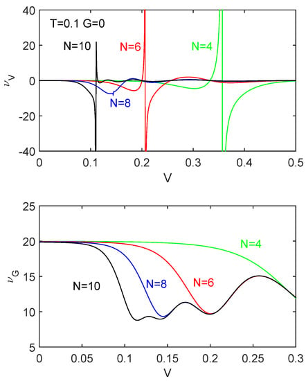
Figure 1. Upper graph: ${\nu }_V$ versus V for $G=0$ for several fermion numbers N. We see that ${\nu }_V$ experiences a sort of discontinuity when V attains a critical value, retaking afterwards its previous value. Lower graph: ${\nu }_G$ versus V for $G=0$. The N values in both plots are r $N=4,6,8,10$, and $T=0.1$.

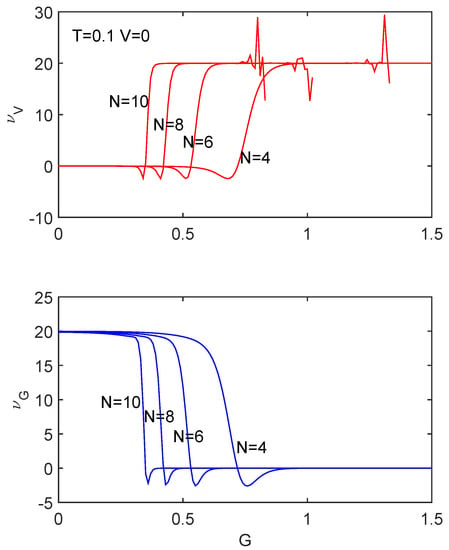
Figure 2. We present two plots $N=4,6,8,10$, $T=0.1$, and $V=0$. Upper graph: ${\nu }_G$ versus V. Lower graph: ${\nu }_G$ versus G.

Figure 1 depicts the order–disorder indicators ${\nu }_V\left(N\right)$ (upper figure) and ${\nu }_G\left(N\right)$ (lower figure) versus V at $T=0.1$ and $G=0$ for different N values. In the first case, there is no energy cost, except at the special critical values $V_{crit}\left(N\right)$, where remnants of the spin–flip phase transitions are evident. We can call these remnants $\nu$ singularities. The moral here is that V critical values are detected by ${\nu }_V$. In the second instance (lower figure), we see clearly how these critical V values affect ${\nu }_G\left(N\right)$ as well. How is this? This is by considerably lowering the associated energy cost of changing G. Thus, we encounter a perhaps unexpected subtle interplay between V and G in the behavior of the energy cost. Finite temperature force V and G interact among themselves.

Let us pass now a quite similar order–disorder panorama, as exhibited by Figure 2, whose protagonists are the variations of the energy cost with G. We see that a similar picture emerges as that provided by Figure 1. The $V-G$ interrelation, a purely statistical interconnection between V and G that is not given by the pertinent Hamiltonian, is at work. First, at the critical G values, the energy cost ${\nu }_V\left(N\right)$ grows. (There is some numerical noise in the graph.) Here, the salient feature is that the energy cost $\nu :G\left(N\right)$ descends to zero at the critical values $G_{crit}$.

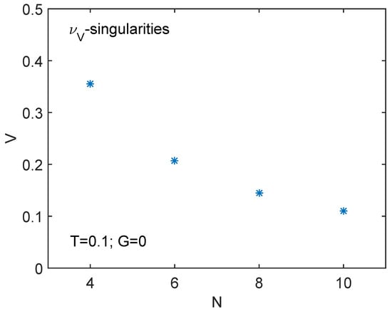
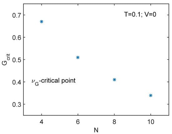
Finally, in Figure 3 and Figure 4, we depict (versus N) the N-dependent critical values of the coupling constants, respectively, $V_{crit}$ and $G_{crit}$. As is well known [1,3], for fixed N, the system displays a spin–flip phase transition at $V_{crit}$ and a superconducting one at $G_{crit}$. Naturally, we speak of “critical values” for the coupling constants. At such values, as we saw above, our statistical quantifiers ${\nu }_G$ and ${\nu }_V$ display “singularities”. Thus, we may say that Figure 3 and Figure 4 display the $\nu$-singularities or critical points versus N, as we state in the captions. The values of these critical points diminish as N grows.

Figure 3. ${\nu }_V$ singularities versus N for $T=0.1$. Their value decreases as N grows.

Figure 4. ${\nu }_G$ singularities versus N for $T=0.1$. Their value decreases as N grows.

7. Conclusions

In the present work, we proceeded as follows.

• First, we established a statistical indicator of order called the disequilibrium D.
• Secondly, we ascertained how much free energy F it takes to change D. The particular $D-$ changes we were interested are those that ensue as a result of variations in the value of the coupling constants of the fermions’ Hamiltonian H.
• The associated free energy costs of having these D variations were quantified via a statistical quantifier, which we called $\nu$ (order variation energy cost).
• Since we have two different interaction terms in H, with coupling constants named V and G, respectively, we had to deal with two different types of $\nu$, which we called ${\nu }_V$ and ${\nu }_G$.
• Finally, we described the behavior of ${\nu }_V$ and ${\nu }_G$ as a function of the number of fermions N. This behavior exhibited interesting features.

Summing up, we here investigated the interconnection between statistical order and disorder. Our main tool to this effect was the new quantifier $\nu$ characterizing alterations in an order–disorder quantifier D. We focused our attention on changes in the total number of fermions N.

More specifically, we analyzed the behavior of $\nu$ when the coupling constants V and/or G underwent modifications and studied how the associated $\nu$ changes depend on N. We compared the statistical order–disorder traits of our two kinds of fermion–fermion interactions. They are indeed different, when analyzed through the lens provided by $\nu$. In particular, they differ in relation to their response to variations in N.

References

- Pennini, F.; Plastino, A. Complexity and disequilibrium as telltales of superconductivity. Physica A 2018, 506, 828–834. [Google Scholar] [CrossRef]
- Cervia, M.J.; Balantekin, A.B.; Coppersmith, S.N.; Johnson, C.W.; Love, P.J.; Poole, C.; Robbins, K.; Saffman, M. Lipkin model on a quantum computer. arXiv 2021, arXiv:2011.04097. [Google Scholar] [CrossRef]
- Balian, R.; Flocard, H.; Veneroni, M. Temperature Dependence of Even-Odd Effects in Small Superconducting Systems. arXiv 1998, arXiv:cond-mat/9802006. [Google Scholar]
- Sedrakian, A.; Clark, J.W. Superfluidity in nuclear systems and neutron stars. Europ. Phys. J. A 2019, 55, 167. [Google Scholar] [CrossRef]
- Lipkin, H.J.; Meshkov, N.; Glick, A.J. Validity of many-body approximation methods for a solvable model: (I). Exact solutions and perturbation theory. Nucl. Phys. 1965, 62, 188–198. [Google Scholar] [CrossRef]
- Lerma, H.S.; Dukelsky, J. The Lipkin-Meshkov-Glick model from the perspective of the SU(1,1) Richardson-Gaudin models. J. Phys. Conf. Ser. 2014, 492, 12013. [Google Scholar] [CrossRef]
- Providencia, C.; da Providencia, J.; Tsue, Y.; Yamamura, M. The Lipkin Model in Many-Fermion System as an Example of the su(1,1) times su(1,1)-Algebraic Model. Prog. Theor. Phys. 2006, 116, 87–105. [Google Scholar] [CrossRef][Green Version]
- Nolting, W. Fundamentals of Many-Body Physics; Springer: Berlin/Heidelberg, Germany, 2009. [Google Scholar]
- Cambiaggio, M.C.; Plastino, A. Quasi spin pairing and the structure of the Lipkin Model. Z. Physik A 1978, 288, 153–159. [Google Scholar] [CrossRef]
- Ring, P.; Schuck, P. The Nuclear Many-Body Problem; Springer: Berlin/Heidelberg, Germany, 1980. [Google Scholar]
- De Llano, M.; Tolmachev, V.V. Multiple phases in a new statistical boson fermion model of superconductivity. Physica A 2003, 317, 546–564. [Google Scholar] [CrossRef]
- Uys, H.; Miller, H.G.; Khanna, F.C. Generalized statistics and high-Tc superconductivity. Phys. Lett. A 2001, 289, 264–272. [Google Scholar] [CrossRef]
- Plastino, A.; Ferri, G.L.; Plastino, A.R. Spectral explanation for statistical odd-even staggering in few fermions systems. Quantum Rep. 2021, 3, 166–172. [Google Scholar] [CrossRef]
- Plastino, A.; Moszkowski, S.M. Simplified model for illustrating Hartree-Fock in a Lipkin-model problem. Nuovo Cimento 1978, 47, 470–474. [Google Scholar] [CrossRef]
- López-Ruiz, R.; Mancini, H.L.; Calbet, X. A statistical measure of complexity. Phys. Lett. A 1995, 209, 321–326. [Google Scholar] [CrossRef]
- López-Ruiz, R. Complexity in some physical systems. Int. J. Bifurc. Chaos 2001, 11, 2669–2673. [Google Scholar] [CrossRef]
- Rudnicki, L.; Toranzo, I.V.; Sánchez-Moreno, P.; Dehesa, J.S. Monotone measures of statistical complexity. Phys. Lett. A 2016, 380, 377–380. [Google Scholar] [CrossRef]
- López-Ruiz, R.; Mancini, H.; Calbet, X. A Statistical Measure of Complexity in Concepts and Recent Advances in Generalized Information Measures and Statistics; Kowalski, A., Rossignoli, R., Curado, E.M.C., Eds.; Bentham Science Books: New York, NY, USA, 2013; pp. 147–168. [Google Scholar]
- Rossignoli, R.; Plastino, A. Thermal effects and the interplay between pairing and shape deformations. Phys. Rev. C 1985, 32, 1040–1048. [Google Scholar] [CrossRef]
- Nigmatullin, R.; Prokopenko, M. Thermodynamic efficiency of interactions in self-organizing systems. Entropy 2021, 23, 757. [Google Scholar] [CrossRef] [PubMed]
Publisher’s Note: MDPI stays neutral with regard to jurisdictional claims in published maps and institutional affiliations. |
© 2022 by the authors. Licensee MDPI, Basel, Switzerland. This article is an open access article distributed under the terms and conditions of the Creative Commons Attribution (CC BY) license (https://creativecommons.org/licenses/by/4.0/).