Quantifying the Effect Size of Exposure-Outcome Association Using δ-Score: Application to Environmental Chemical Mixture Studies

Abstract

Epidemiologists often study the associations between a set of exposures and multiple biologically relevant outcomes. However, the frequently used scale-and-context-dependent regression coefficients may not offer meaningful comparisons and could further complicate the interpretation if these outcomes do not have similar units. Additionally, when scaling up a hypothesis-driven study based on preliminary data, knowing how large to make the sample size is a major uncertainty for epidemiologists. Conventional p-value-based sample size calculations emphasize precision and might lead to a large sample size for small- to moderate-effect sizes. This asymmetry between precision and utility is costly and might lead to the detection of irrelevant effects. Here, we introduce the “$\delta$-score” concept, by modifying Cohen’s $f^2$. $\delta$-score is scale independent and circumvents the challenges of regression coefficients. Further, under a new hypothesis testing framework, it quantifies the maximum Cohen’s $f^2$ with certain optimal properties. We also introduced “Sufficient sample size”, which is the minimum sample size required to attain a $\delta$-score. Finally, we used data on adults from a 2017–2018 U.S. National Health and Nutrition Examination Survey to demonstrate how the $\delta$-score and sufficient sample size reduced the asymmetry between precision and utility by finding associations between mixtures of per-and polyfluoroalkyl substances and metals with serum high-density and low-density lipoprotein cholesterol.

1. Introduction

Estimating an effect size with high precision is the essence of epidemiological research, so when given a hypothesis with specific aims, preliminary data is collected. But this can be costly, as can processing biological samples; therefore, this stage protects against the waste of resources should the study does not progress as planned. Next depending on the effect estimate and resource constraints, a larger study is planned. For example, consider a scenario where an epidemiologist wants to study the association between perfluoroalkyl and polyfluoroalkyl substances (PFAS) and liver enzyme alanine aminotransferase (ALT) and cytokeratin-18 (CK-18), a marker of liver-cell death in school-age children.

PFAS belong to a diverse class of environmental pollutants of “emerging concern” because they interfere with multiple metabolic and hormonal systems in humans [1]. ALT and CK-18 may or may not be measured in similar units, and they quantify different aspects of liver injury. Although animal studies have shown a biologically plausible cause-effect relationship between PFAS exposure and increased ALT/CK-18 levels, their associations in humans are not well studied ([2,3]).

Now, let us assume that the regression estimate for both the associations is a two-unit increase for every unit increase in PFAS. If the units of ALT and CK-18 are different, comparing these estimates is difficult. Even a conversion to scale-free outcomes makes the interpretation non-intuitive. Further, if ALT and CK-18 are measured in same scale, a two-unit increase in one would have very different clinical and practical implications to a similar increase in the other, because one has a higher potential for public health intervention. Moreover, it was assumed that none of these associations is statistically significant at the current sample size. Based on this hypothesis, the epidemiologist decided to scale up the study and apply for a grant based on the preliminary data. A p-value based sample-size calculation yielded large and comparable sample sizes with corresponding statistically significant effect sizes. This situation led to some quandaries. First, the increased precision due to a larger sample size may not indicate a meaningful effect size, but it would guarantee that any irrelevant or tiny effect sizes would be detectable ([4,5]). Second, for a meaningful and statistically significant effect size, this high precision may not be needed if the effect size does not change considerably with sample size increases. Moreover, measuring PFAS/ALT/CK-18 in child serum is time consuming and costly; therefore, if the effect estimate allows for a contextual, biological or clinical implication, even for a small-to-moderate sample size, there would be no need to increase the sample size without a strong justification for higher precision. Therefore a p-value based association analysis further deepens the asymmetry between precision and utility.

A long established index for reporting the strength of an explanatory association is Cohen’s $f^2$ [6], which evaluates the impact of additional variables over baseline covariates. Over the past three decades, Cohen’s $f^2$ has been used extensively in the behavioral, psychological, and social sciences because of its immense practical utility and ease of interpretation [7]. A similar treatment for scale-free effect-size methodologies can be found in [8,9]. Analogous ideas like genome-wide complex trait analysis are widely used in genome-wide association studies to estimate heritability ([10,11]). In environmental epidemiology, ref. [12] recently introduced the idea of total explained variation (TEV) approach to estimate an overall effect for highly correlated mixtures of exposures using a p-value-based inference. In this paper, we propose a $\delta$-score by modifying Cohen’s $f^2$ to evaluate the strength of the explanatory association in a more fundamental and scale-independent way. Similar to Cohen’s $f^2$, the $\delta$-score moves the contextual reference to baseline covariates and evaluates the effect size contributed solely by a set of exposures or exposure-mixtures on top of those baseline covariates. Further, under a special hypothesis-testing framework, we show that the $\delta$-score quantifies the maximum Cohen’s $f^2$ and admits some useful optimal properties. The idea was naturally extended to a new concept, “Sufficient sample size", which is an estimate of the minimum sample size required to attain a $\delta$-score.

Through illustrative examples and application in 2017–2018 U.S. National Health and Nutrition Examination Survey (NHANES) data, we quantified $\delta$-scores and sufficient sample sizes for associations between mixtures of PFAS and metals on lipoprotein-cholesterols and demonstrated that sufficient sample sizes are usually smaller than the p-value-based sample-size estimates.

2. Methods

A common problem of testing occurs when a set of exposures in a regression model is associated with the outcome after adjusting for covariates and confounders. For example, consider the linear model, $y=X_0{b}_0+X_1{b}_1+\epsilon$: we want to find out the strength of the association of $X_1$ after adjusting for $X_0$ and to compare hypothesis $H_0(\mathrm{Effect}\mathrm{size}\mathrm{due}\mathrm{to}{X}_1=0$) with hypothesis $H_1(\mathrm{Effect}\mathrm{size}\mathrm{due}\mathrm{to}{X}_1=\delta$), where $\delta$ is a positive and pre-defined meaningful quantity. In the sections below, we briefly discuss Cohen’s $f^2$ in linear regression and then move on to formulate an error-calibrated hypothesis-testing framework. Lastly, we introduce the idea of the $\delta$-score and sufficient sample size under that framework.

2.1. Cohen’s $f^2$ in Linear Regression

Consider the linear regression model noted above and assume $ϵ\sim N(0,{\sigma }^2{I}_n)$, where $I_n$ is an identity matrix of dimension $n\times n$. Let ${\gamma }_n$ be the non-centrality parameter, then ${\gamma }_n$ equals 0 when y is generated under $H_0$. When y is generated under the alternative, ${\gamma }_n$ has the form of ${\gamma }_n=\frac{\parallel \left(I_n-P_{X_0}\right)X_1{b}_1{\parallel }^2}{{\sigma }^2}$, where $P_{X_0}=X_0{\left({X_0}^{\top }{X}_0\right)}^{-1}{X}_0^{\top }$ is the projection matrix onto the linear space spanned by the column vectors of $X_0$ ([13,14]) (see Section S1 of the Supplementary Materials). For the typical regression design in which the predictor vector of each subject is drawn from a common population, ${\gamma }_n$ grows linearly on n. Note that ${\gamma }_n$ does not depend on y but rather on the design matrix X and underlying parameters $b_1$ and ${\sigma }^2$. A long-established index of quantifying additional impact in linear regression is Cohen’s $f^2$,

$$f^2=\frac{R_{y,X_0,X_1}^2-R_{y,X_0}^2}{1-R_{y,X_0,X_1}^2},$$

where $R_{y,X_0,X_1}^2$ and $R_{y,X_0}^2$ are the squared multiple correlations for $X_0,X_1$ under $H_1$ and $X_0$ under $H_0$, respectively. $f^2$ quantifies the proportion of variation in y accounted for by $X_1$ on top of the variation accounted for by $X_0$, a concept most researchers can relate to intuitively [15]. In linear regression, Cohen’s $f^2$ and non-centrality parameter ${\gamma }_n$ can be connected through Lemma 1.

Lemma 1.

$$\frac{n{f}^2}{{\gamma }_n}\underset{n\to \infty }{\overset{P}{\to }}1,$$

where the notation $\underset{n\to \infty }{\overset{P}{\to }}$ denotes convergence in probability. See the proof in Section S2 of the Supplementary Materials. Further discussion on Cohen’s $f^2$ in generalized linear models is presented in Section S3 of the Supplementary Materials.

2.2. Formulation of Error Calibrated Cutoff in a New Hypothesis Testing Framework

Following the hypothesis in (1) and for a meaningful value of $\delta >0$, we specify our main hypothesis:

$$H_0:f^2=0\mathrm{vs}.H_1:f^2=\delta .$$

(1)

Let ${\widehat{b}}_{0,H_0}$ be the maximum likelihood estimate (MLE) for a model with only design matrix $X_0$, and let ${\widehat{b}}_{0,H_1}$ and ${\widehat{b}}_{1,H_1}$ be the MLEs for the model with design matrices $X_0$ and $X_1$. The standard test to compare a null and alternative is through F statistic, $F\left(y\right)=\frac{({\mathrm{SSR}}_0-{\mathrm{SSR}}_1)/p_1}{{\mathrm{SSR}}_1/(n-p_0-p_1)}$, where ${\mathrm{SSR}}_0={(y-X_0{\widehat{b}}_{0,H_0})}^t(y-X_0{\widehat{b}}_{0,H_0})$ is the sum of the squared errors under $H_0$, and ${\mathrm{SSR}}_1={(y-X_0{\widehat{b}}_{0,H_1}-X_1{\widehat{b}}_{1,H_1})}^t(y-X_0{\widehat{b}}_{0,H_1}-X_1{\widehat{b}}_{1,H_1})$ is the sum of the squared errors under $H_1$. Then $F\left(y\right)\sim F_{p_1,n-p_0-p_1}\left({\gamma }_n\right)$, where $p_1$ and $n-p_0-p_1$ are degrees of freedom and ${\gamma }_n$ is the non-centrality parameter. When the data is generated under the null or the alternative hypothesis, and, as $n\to \infty$ while $p_0,p_1$ remain fixed, this F distribution can be approximated by the chi-squared distribution ${lim}_{n\to \infty }{p}_{1}F\left(y\right)\sim {\chi }_{p_1}^2\left({\gamma }_n\right)$. On the other hand, suppose that the likelihood ratio test statistic for testing this hypothesis is, $\Lambda \left(y\right)=2\left\{\ell ({\widehat{b}}_{1,H_1},{\widehat{b}}_{0,H_1}|X_0,X_1)-\ell \left({\widehat{b}}_{0,H_0}\right|X_0)\right\}$. As the sample size $n\to \infty$, the likelihood ratio statistic $\Lambda \left(y\right)$ follows a central chi-squared distribution ${\chi }_{p_1}^2$ with $p_1$ degrees of freedom when y is generated under the model in $H_0$. $\Lambda \left(y\right)$ follows a non-central chi-squared distribution ${\chi }_{p_1}^2\left({\gamma }_n\right)$ with degrees of freedom $p_1$ and non-centrality parameter ${\gamma }_n$ when y is generated under $H_1$.

Let the test statistic $S\left(y\right)=p_{1}F\left(y\right)$ for a linear regression and $S\left(y\right)=\Lambda \left(y\right)$ for other generalized linear models. These specifications are motivated by the fact that $S\left(y\right)$ asymptotically follows a chi-squared distribution. Let, T be a cutoff value which depends on sample size n and unknown parameters $p_1$ and effect size $\delta$. Then, given a cutoff value T and based on hypothesis (1), the type 1 error $\alpha \left(\mathrm{T}\right)$ can be expressed as $P\left(S\left(y\right)>\mathrm{T}\mid f^2=0\right)$, and the type 2 error $\beta \left(\mathrm{T}\right)$ can be expressed as $P\left(S\left(y\right)<\mathrm{T}\mid f^2=\delta \right)$. Such specification of type 1 and type 2 errors is inspired by model selection procedures, Akaike’s information criterion [16] and the Bayesian information criterion [17], which are often used in place of hypothesis testing for choosing between competing models [18]. As a consequence, given the error calibrated cutoff value of T, we have

$$\begin{array}{cc}\hfill \alpha \left(\mathrm{T}\right)& =P\left(S\left(y\right)>\mathrm{T}\mid f^2=0\right)=P\left({\chi }_{p_1}^2>\mathrm{T}\right)\hfill \\ \hfill \beta \left(\mathrm{T}\right)& =P\left(S\left(y\right)<\mathrm{T}\mid f^2=\delta \right)=P\left({\chi }_{p_1}^2\left({\gamma }_n\right)<\mathrm{T}|{\gamma }_n=n\delta \right).\hfill \end{array}$$

Our central idea was to choose T so that the type 1 error $\alpha \left(\mathrm{T}\right)$ and the type 2 error $\beta \left(\mathrm{T}\right)$ satisfied the relationship, $\alpha \left(\mathrm{T}\right)=\theta \beta \left(\mathrm{T}\right)$, with $0<\theta <\infty$, and $\theta$ is pre-specified. Using the chi-square approximation to $S\left(y\right)$, we solved for the calibrated cutoff value T by equation

$$P\left({\chi }_{p_1}^2>\mathrm{T}|{\gamma }_n=0\right)=\theta P\left({\chi }_{p_1}^2\left({\gamma }_n\right)<\mathrm{T}|{\gamma }_n=n\delta \right).$$

(2)

When T is fixed, the left side of Equation (2) remains constant as $n\to \infty$, while the right side diminishes to 0 rapidly under the non-centrality parameter $n\delta$. Therefore, Equation (2) implies $\mathrm{T}\to \infty$ as $n\to \infty$. In Theorem 1 stated below, we elaborate more on T. The results in this theorem depend on the normality approximation of the non-central chi-square distribution; that is, for large n, Equation (2) was rewritten as

$$P\left({\chi }_{p_1}^2>\mathrm{T}|{\gamma }_n=0\right)=\theta \Phi \left(\frac{\mathrm{T}-p_1-n\delta }{\sqrt{2(p_1+2n\delta )}}\right),$$

(3)

where, $\Phi (.)$ denotes the cumulative density function of a standardized normal random variable. For ease of interpretation and theoretical derivations, we considered $\theta =1$ in the following sections when both the type 1 and type 2 errors decay at the same rate. The cases with $\theta \ne 1$ can be developed similarly.

Theorem 1.

Consider the hypothesis of interest $H_0:f^2=0vs.H_1:f^2=\delta$ where $f^2$ denotes Cohen’s $f^2$. Assume response vector y is generated under the alternative. Then following the constraint $\alpha \left(T\right)=\beta \left(T\right)$, as in (2) and for large n, the error calibrated cutoff value T has the expression

$$T=\left(\frac{\delta n}{2K-1}+c_1{n}^{\frac{1}{2K}}\right)(1+o\left(1\right)).$$

(4)

Further, the type 1 or type 2 error rates can be expressed as

$$\begin{array}{c}\hfill \frac{d}{dn}log\left\{\alpha \left(T\right)\right\}=\frac{d}{dn}log\left\{\beta \left(T\right)\right\}=-\frac{\delta {(K-1)}^2}{2{(2K-1)}^2}+o\left(1\right),\end{array}$$

(5)

where $K\to (2+\sqrt{2})(1+o\left(1\right))$ and $c_1$ is a constant of integration.

The proof is presented in Section S4 of the Supplementary Materials, and in Section S4.2 the explicit expressions of $log\left\{\alpha \right(T\left)\right\}$ and $log\left\{\beta \right(T\left)\right\}$ are derived. Theorem 1 sheds light on the behavior of the cutoff value T and the rates of the corresponding type 1 or type 2 errors when the sample size n is large. Since both errors tended to 0 as $n\to \infty$, this procedure for testing the hypothesis was consistent and kept error rates equal. It should be noted that both errors decayed at an exponential rate even at moderate sample sizes. To gauge the accuracy of Theorem 1, we presented the type 1 and type 2 error rates and the rate of change of T with respect to n using the results from Theorem 1 and the corresponding numerical results from Equation (3). As seen in Table 1, irrespective of Cohen’s $f^2$, as n increased, the rate of change of T, log (type 1) and log (type 2) converged to the corresponding theoretical rates specified in Theorem 1. We also conducted a Monte Carlo simulation to estimate the calibrated type 1 and type 2 errors for different values of n, $p_1$ and $f^2$ (see Section S5 and Table S1 of the Supplementary Materials). Moreover, a detailed discussion of the properties of the error calibrated cutoff T and the type 2 error is presented in Section S6 of the Supplementary Materials.

Table 1. Rates of cutoff value T, log (type 1) or log (type 2) with respect to sample size n based on Equation (3) and Theorem 1.

			Numerical Approximation Using		Using Theorem
			Equation (3)		(1)
${\mathit{p}}_{\mathbf{1}}$	${\mathit{f}}^{\mathbf{2}}$	$\mathit{n}$	$\frac{\mathit{d}}{\mathit{d}\mathit{n}}T$	$\frac{\mathit{d}}{\mathit{d}\mathit{n}}log\left(\mathbf{\alpha }\right)$	$\frac{\mathit{d}}{\mathit{d}\mathit{n}}T$	$\frac{\mathit{d}}{\mathit{d}\mathit{n}}log\left(\mathbf{\alpha }\right)$
1	$2.5\%$	250	0.0042895	−0.0031	0.0042893	−0.0021
1	$10\%$	250	0.0171573	−0.0100	0.0171573	−0.0086
5	$2.5\%$	250	0.0043764	−0.0025	0.0042893	−0.0021
5	$10\%$	250	0.0172491	−0.0090	0.0171573	−0.0086
1	$2.5\%$	500	0.0042896	−0.0028	0.0042893	−0.0021
1	$10\%$	500	0.0171573	−0.0094	0.0171573	−0.0086
5	$2.5\%$	500	0.0043764	−0.0024	0.0042893	−0.0021
5	$10\%$	500	0.0172491	−0.0087	0.0171573	−0.0086

2.3. Notion of $\delta$-Score

We can borrow the convention for $f^2$ [6] and call $f^2\ge 0.02$, $f^2\ge 0.15$ and $f^2\ge 0.35$ as representing small, moderate, and large effect sizes, respectively. This can serve as a guide to understating the effect size obtained from the data. Further, given the data, one can use this hypothesis by sequentially choosing and testing increasing values of $\delta$ as long as the null is rejected and stops when the it can no longer be rejected. Finally, this brings us to the question of whether, given any data, there exists any maximum $\delta$ such that the null will always be rejected. Let the likelihood ratio test statistic be $\Lambda \left(y\right)$. We reject the null if and only if $T\left(\delta \right)\le \Lambda \left(y\right)$. Hence, $T\left(\delta \right)$ attains a maximum at the upper bound $\Lambda \left(y\right)$. Denote this $\delta -$ value at which $T\left(\delta \right)$ attains the maximum value as ${\delta }^{\ast }$, and consider the reformulated hypothesis (1) as below, with ${\delta }^{\ast }$ as the final choice of $\delta$:

$$H_0:f^2=0\mathrm{vs}.H_1:f^2={\delta }^{\ast }.$$

(6)

We note some interesting properties of ${\delta }^{\ast }$ through the following corollary,

Corollary 1.

Under the hypothesis in (6), let ${\delta }^{\ast }$ be the unique solution to the equation $T\left({\delta }^{\ast }\right)=\Lambda \left(y\right)$. Therefore, ${\delta }^{\ast }$ admits the following properties:

• ${\delta }^{\ast }$ is the maximum value of Cohen’s $f^2$ such that the null is still rejected.
• For any $h\ge -{\delta }^{\ast }$, the asymptotic type 1 error, $P\left({\chi }_{p_1}^2>T({\delta }^{\ast }+h)|{\gamma }_n=0\right)$ is a monotonically decreasing function of h, whereas the asymptotic type 2 error,
  $P\left({\chi }_{p_1}^2\left({\gamma }_n\right)<T({\delta }^{\ast }+h)|{\gamma }_n=E_y\left\{\Lambda \left(y\right)\right\}\right)$ is a monotonically increasing function of h.

See the proof in Section S8 of Supplementary Materials. Further, for large n, ${\delta }^{\ast }$ undertakes asymptotic convergence (Lemma 3.1 of [19]), and we define “$\delta$-score” as noted below:

$$\delta -\mathrm{score}:=E_y\left\{{\delta }^{\ast }\right\},n\to \infty .$$

Under the hypothesis-testing framework in (1), $\delta$-score captures the asymptotic and maximum Cohen’s $f^2$, which was contributed solely by the larger exposure model on top of the baseline covariate-only model. Unlike usual null hypothesis significance testing based on sequential testing [20], this framework does not inflate the type 1 error and circumvents the issue through its use of the error calibrated cutoff value and keeps the error rates in balance. Instead of simply estimating Cohen’s $f^2$, this procedure introduces hypothesis testing for error-balanced decision making.

One might use hypothesis (1) solely for testing, since, under the error calibrated framework it induces an expanded null hypothesis which nicely connects to the interval null hypothesis in the literature ([21,22,23,24]). This expanded null hypothesis guards against near-certain rejection of the null when the sample size is large enough and the null is true (see Section S6 of Supplementary Materials). Although the $\delta$-score can be interpreted through the lens of this hypothesis, it should be primarily used only for estimations and comparisons. The reason is that, for a set of exposures and their corresponding outcome, the $\delta$-score signifies the maximum Cohen’s $f^2$ that can be attained within the possible zone of rejection. Therefore, the $\delta$-score concept is firmly rooted in the rejection interval no matter the effect size; however, since Cohen’s $f^2$ cannot be larger than the $\delta$-score within this region, the $\delta$-score facilitates comparisons among multiple outcomes.

2.4. Notion of Sufficient Sample Size

The $\delta$-score can be estimated by bootstrapping a large sample size N (say $N=5000$ or $10,000$) with replacement from the original sample of size n, with $n<N$. Moreover, because of its convergence, one can find a much smaller bootstrapped sample size and corresponding estimated $\delta$-score such that it will be in the “practically close neighborhood” of the converged $\delta$-score based on a considerably large bootstrap size. We defined the smaller bootstrapped size as a “Sufficient sample size”.

Consider the equivalence tests for the ratio of two means with prespecified equivalence bounds ([25,26]). Let ${\delta }^s$ and ${\delta }^{\mathrm{opt}}$ be the underlying random variables for two separate $\delta$-scores to be estimated under sample sizes N and $n_s$, respectively. To formulate the test of non-equivalence between these two estimated $\delta$-scores, consider this hypothesis:

$$\begin{array}{cc}\hfill H_0& :\mu \left(log\left\{\frac{{\delta }^s}{{\delta }^{opt}}\right\}\right)<l_R\mathrm{or}\mu \left(log\left\{\frac{{\delta }^s}{{\delta }^{opt}}\right\}\right)>l_U\mathrm{vs}.H_1:l_R\le \mu \left(log\left\{\frac{{\delta }^s}{{\delta }^{opt}}\right\}\right)\le l_U,\hfill \end{array}$$

(7)

where, $l_R$ and $l_U$ are the lower and upper equivalence bounds with $l_R<0$ and $l_U>0$. The null hypothesis will be rejected to favour the alternative if a two-sided $100(1-2\alpha )\%$ CI is completely included within $l_R$ and $l_U$. We will assume $l_R=log\left(0.8\right)$ and $l_U=log\left(1.25\right)$ following typical practice [27], but less strict values can be chosen for practical purposes. $\mu \left(\frac{{\delta }^s}{{\delta }^{opt}}\right)$ and $\sigma \left(\frac{{\delta }^s}{{\delta }^{opt}}\right)$ are approximated by using Taylor series expansions (detailed in Section S2 of the Supplementary Materials). The mean and variance after logarithmic transformation are found using direct application of the delta theorem on $\frac{{\delta }^s}{{\delta }^{opt}}$. Finally, we declared an alternative hypothesis if the $2\alpha$ level CI on $\mu \left(log\left\{\frac{{\delta }^s}{{\delta }^{opt}}\right\}\right)$ were within the equivalence limits:

$$\begin{array}{cc}\hfill l_R& \le log\left(\widehat{\mu }\left\{\frac{{\delta }^s}{{\delta }^{opt}}\right\}\right)-\frac{t_{1-\alpha ,M-1}}{\sqrt{M}}\frac{\widehat{\sigma }\left(\frac{{\delta }^s}{{\delta }^{opt}}\right)}{\widehat{\mu }\left(\frac{{\delta }^s}{{\delta }^{opt}}\right)}\mathrm{and}log\left(\widehat{\mu }\left\{\frac{{\delta }^s}{{\delta }^{opt}}\right\}\right)+\frac{t_{1-\alpha ,M-1}}{\sqrt{M}}\frac{\widehat{\sigma }\left(\frac{{\delta }^s}{{\delta }^{opt}}\right)}{\widehat{\mu }\left(\frac{{\delta }^s}{{\delta }^{opt}}\right)}\le l_U,\hfill \end{array}$$

where $t_{1-\alpha ,M-1}$ is the $100{(1-\alpha )}^{\mathrm{th}}$ percentile in a standard t-distribution. As long as the hypothesis of non-equivalence in (7) is rejected in favour of the alternative, $n_s$ can be regarded as a “sufficient sample size” at equivalence bounds of $[log\left(\frac{8}{10}\right),log\left(\frac{10}{8}\right)]$ with a corresponding $\delta$-score of $\widehat{\mu }\left({\delta }^s\right)$. Ratio type estimators such as discussed above can be further improved by involving either first or third quartile of the corresponding auxiliary variable (see [28] for further details).

3. Illustration with a Simulated Example

Consider a normally distributed outcome and one single exposure with five baseline covariates with a sample size of 300. Further assume that the $R^2$ for the baseline covariate-only model is $20\%$, and the true and unknown $\delta$-score due to the exposure is $5.8\%$. Therefore, the $R^2$ for the larger model with a single exposure and five covariates is $20.8\%$ (the mean correlation between the covariates is set at $0.3$, and the error variance is assumed to be 5). See Section S7 of the Supplementary Materials for the data generating process.

Assume a researcher collected these data and intends to find the association between the outcome and exposure after controlling for the five baseline covariates. As a first step, the $\delta$-score is estimated by bootstrapping a sample of size $N=5000$ from an original sample size of $n=300$. The estimated $\delta$-score is $6.1\%$, which is very close to the true $\delta$-score of $5.8\%$). Similarly, the $\delta$-scores are estimated at bootstrapped sample sizes $N=200,300,400,500,600$, and 2500 to illustrate the gradual convergence as the bootstrap size increases (Figure 1A). Further note that even when precision increased with bootstrap size, the mean of regression coefficients remained stable (Figure 1B) while the p-values from linear regression keep getting smaller (Figure 1C). Moreover, the power based on the likelihood ratio test and corresponding calibrated cutoff value of $\mathrm{T}(p_1,n,\delta )$ kept increasing rapidly (Figure 1D).

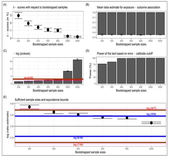
Figure 1. Results from simulated example. (A) Illustration of $\delta$-scores for different bootstrapped sample sizes and their eventual convergence, (B) Mean $\beta$ estimates and standard errors of the exposure–outcome association, (C) Negative log (base = e) p-values as bootstrapped sample sizes increased, (D) Power of the likelihood ratio test based on the calibrated cutoff value $\mathrm{T}(n,p_1,\delta )$, and (E) Sufficient sample sizes concerning the choices of equivalence bounds.

For the original sample size of $n=300$, the corresponding p-value of the regression estimate was not significant. The researcher, therefore, might have wanted to scale up the study to collect more data and increase the original sample size based on statistical power calculation and sample size determination, which estimated that a sample size of around 1000 was required assuming $80\%$ power of the test and the type 1 error was fixed at $5\%$. Sufficient sample-size estimation using $\delta$-score struck a balance between precision and utility. We estimated $\mu \left(log\left\{\frac{{\delta }^s}{{\delta }^{opt}}\right\}\right)$ based on 2000 iterations and used the non-equivalence hypothesis in (7) to compare the $\delta$-scores at $N=200,300,400,500,600$, and 2500 with respect to the estimated $\delta$-score at $N=5000$ (Figure 1E). At $N=600$, $\mu \left(log\left\{\frac{{\delta }^s}{{\delta }^{opt}}\right\}\right)$ and its $95\%$ CI lie within the bounds of $l_R=log(8/10)$ and $l_U=log(10/8)$, whereas at $N=500,400$ and 300, it breached the upper bound of $l_U=log(10/8)$ but stayed within the bounds of $l_R=log(7/10)$ and $l_U=log(10/7)$. Accordingly, the researcher can choose a sufficient sample size of $N=600$ or $N=300$ at equivalence bounds of $[log(8/10),log(10/8\left)\right]$ or $[log(7/10),log(10/7\left)\right]$, respectively, with corresponding $\delta$-scores of $7\%$ and $7.9\%$. These $\delta$-scores were within a close neighborhood of the converged $\delta$-scores of $6\%$ (based on the bootstrapped size of $N=5000$).

4. Application in Exposure–Mixture Association of PFAS and Metals with Serum Lipids among US Adults

PFAS are exclusively artificial endocrine disrupting chemicals (EDCs) and environmentally persistent chemicals that are used to manufacture a wide variety of consumer and industrial products: non-stick, stain, and water resistant coatings; fire suppression foam; and cleaning products ([29,30]). Both PFAS and metals have been associated with an increase in cardiovascular disease (CVD) or death as evidenced by many cross-sectional and longitudinal observational studies and experimental animal models [31]. Hypercholesterolemia is one of the significant risk factors for CVD characterized by high levels of serum cholesterol. High levels of low-density lipoprotein (LDL), total serum cholesterol, and low levels of high-density lipoprotein (HDL) are some of the factors implicated in the pathogenesis of this disorder [32]. Using the theory discussed in the sections above, we quantified the $\delta$-scores of PFAS and metal mixtures on serum lipoprotein cholesterols and estimated corresponding sufficient sample sizes.

4.1. Study Population

Using cross-sectional data from the 2017–2018 U.S. NHANES [33], this study used data on 683 adults. Data on baseline covariates–––age, sex, ethnicity, body mass index (BMI) (in kg/m${}^2$), smoking status, and ratio of family income to poverty—were downloaded and matched to the IDs of the NHANES participants. See Table 2 for details on participant characteristics. A weight variable was added in the regression models to adjust for oversampling of non-Hispanic black, non-Hispanic Asian, and Hispanic in this NHANES data. A list of individual PFAS, metals, and their lower detection limits can be found in Section S9 in the Supplementary Materials.

Table 2. Study characteristics of the population under investigation. (Data from National Health and Nutrition Examination Survey 2017–2018.)

	Total	Male	Female	% Observations ≥ LLOD
Sample size (n)	683	339	344
Baseline Covariates
Age (years)	49.51 (18.77)	50.38 (18.81)	48.65 (18.73)
Ethnicity
Mexican American	88	43 (49%)	45 (51%)
Other Hispanic	58	23 (40%)	35 (60%)
Non-Hispanic White	260	135 (52%)	125 (48%)
Non-Hispanic Black	155	79 (51%)	76 (49%)
Other Race—Including Multi-Racial	122	59 (48%)	63 (52%)
Body mass index (kg/m${}^2$)	29.59 (7.90)	28.67 (6.36)	30.49 (9.09)
Smoking Status
Never	402	170 (42%)	232 (58%)
Smoked at least 100 cigarettes
but doesn’t smoke now	163	100 (61%)	63 (39%)
Smoked at least 100 cigarettes
and still smokes now	118	69 (58%)	49 (42%)
Ratio of family income to poverty	2.56 (1.61)	2.64 (1.63)	2.48 (1.59)
Outcomes
HDL-C (mg/dL)	53.91 (15.53)	49.19 (13.10)	58.56 (16.33)
LDL-C (mg/dL)	109.35 (37.11)	108.99 (35.35)	109.71 (38.83)
PFAS exposures (Unadjusted geometric means with 95% confidence intervals)
PFDeA (ng/mL)	0.20 (0.19, 0.21)	0.21 (0.19, 0.22)	0.20 (0.18, 0.22)	68.73 %
PFHxS (ng/mL)	1.10 (1.03, 1.17)	1.49 (1.38, 1.61)	0.81 (0.74, 0.89)	99.12%
Me-PFOSA-AcOH (ng/mL)	0.13 (0.12, 0.14)	0.14 (0.13, 0.15)	0.12 (0.11, 0.13)	38.64%
PFNA (ng/mL)	0.42 (0.39, 0.44)	0.46 (0.42, 0.5)	0.38 (0.34, 0.42)	91.74%
PFUA (ng/mL)	0.14 (0.13, 0.15)	0.14 (0.13, 0.15)	0.14 (0.13, 0.15)	41.59%
n-PFOA (ng/mL)	1.28 (1.22, 1.35)	1.52 (1.42, 1.64)	1.08 (1, 1.17)	99.41%
n-PFOS (ng/mL)	3.26 (3.04, 3.5)	4.11 (3.74, 4.51)	2.59 (2.35, 2.86)	99.41%
Sm-PFOS (ng/mL)	1.28 (1.19, 1.37)	1.73 (1.58, 1.89)	0.95 (0.86, 1.04)	98.82 %
Lead, Cadmium, Total Mercury, Selenium, & Manganese exposures
(Unadjusted geometric means with 95% confidence intervals)
Cd ($\mathsf{\mu }$g/L)	0.32 (0.3, 0.34)	0.29 (0.27, 0.32)	0.35 (0.32, 0.38)	91.36%
Pb ($\mathsf{\mu }$g/dL)	0.91 (0.86, 0.96)	1.09 (1, 1.18)	0.76 (0.7, 0.82)	100%
Mn ($\mathsf{\mu }$g/L)	9.45 (9.21, 9.7)	8.91 (8.62, 9.22)	10.01 (9.64, 10.41)	100%
THg ($\mathsf{\mu }$g/L)	0.78 (0.72, 0.84)	0.81 (0.73, 0.9)	0.75 (0.67, 0.83)	84.77%
Se ($\mathsf{\mu }$g/L)	188.62 (186.75, 190.52)	189.28 (186.57, 192.04)	187.97 (185.38, 190.6)	100%

Data presented as mean (SD) or n(%); LLOD: lower limit of detection; LDL-C: low-density lipoproteincholesterol (mg/dL); HDL-C: high-density lipoprotein-cholesterol (mg/dL); PFDeA: Perfluorodecanoic acid; PFHxS: Perfluorohexane sulfonic acid; Me-PFOSA-AcOH: 2-(N-methylperfluoroctanesulfonamido)acetic acid; PFNA: Perfluorononanoic acid; PFUA: Perfluoroundecanoic acid; PFDoA: Perfluorododecanoic acid; n-PFOA: n-perfluorooctanoic acid; Sb-PFOA: Branch perfluorooctanoic acid isomers; n-PFOS: n-perfluorooctane sulfonic acid; Sm-PFOS: Perfluoromethylheptane sulfonic acid isomers; Pb: Lead; Cd: Cadmium; THg: Total Mercury; Se: Selenium; Mn: Manganese.

4.2. Methods

We used weighted quantile sum regression [34], but other exposure mixture models such as Bayesian kernel machine regression [35], Bayesian weighted quantile sum regression [36], and Quantile g-computation [37] can also be used, as long as the likelihood ratio test statistic can be estimated (see [11,38] for a detailed discussion on exposure–mixture methods in environmental epidemiology). All the PFAS and metals were converted to decile. As an additional analysis, both serum cholesterols were dichotomized using their 90th percentile, to demonstrate the effectiveness of $\delta$-scores on binary outcomes. $\delta$-scores were estimated using bootstrapped sizes of 5000 from the original sample size of 683, and the process was iterated 100 times.

4.3. Results

For metals and PFAS, the $\delta$-scores of continuous HDL-C were $9.6\%[95\%$ CI: $(9.1\%,10.0\%)]$ and $10.7\%[95\%$ CI: $(10.2\%,11.1\%)]$, respectively, whereas for continuous LDL-C, the scores were $14.7\%[95\%$ CI: $(14.2\%,15.2\%)]$ and $16.2\%[95\%$ CI: $(15.6\%,16.7\%)]$, respectively. Both mixtures had relatively higher $\delta$-scores on LDL-C than HDL-C. Furthermore, for both cholesterols, the metal mixture had a slightly higher $\delta$-score than the PFAS mixture (Figure 2A,B). PFAS and Metal mixtures have higher $\delta$-scores for LDL-C than HDL-C. Further, after dichotomizing the cholesterols at their 90th percentile, the $\delta$-scores for the metal mixture remained similar to the continuous cholesterol outcome (HDL-C: $9.8\%[95\%$ CI: $(9.4\%,10.2\%)]$ and LDL-C: $17.2\%[95\%$ CI: $(16.6\%,17.8\%)]$), but decreased slightly for the PFAS mixture (HDL-C: $6.9\%[95\%$ CI: $(6.5\%,7.2\%)]$ and LDL-C: $11.5\%[95\%$ CI: $(11.0\%,12.0\%)]$). The decrease might have been due to some loss of information during dichotomizing the outcomes (Figure 2C,D).

Figure 2. $\delta$-scores of EDC exposure–mixture of metals and PFAS for continuous (A,B) and dichotomized (C,D) serum lipoprotein–cholesterols.

Sufficient sample sizes were also estimated for this dataset at the equivalence bounds of $[log\left(\frac{75}{100}\right)$, $log\left(\frac{100}{75}\right)]$. For both metal and PFAS mixtures, the $\mu \left(log\left\{\frac{{\delta }^s}{{\delta }^{opt}}\right\}\right)$ and their corresponding $95\%$ CIs for bootstrap size 683, lay well within the equivalence bounds. Further, even at a decreased sample size of 483, the $\mu \left(log\left\{\frac{{\delta }^s}{{\delta }^{opt}}\right\}\right)$ and their $95\%$ CIs, remained within the equivalence bounds. Therefore, $N=483$ is a sufficient sample size at equivalence bounds $[log\left(\frac{75}{100}\right)$, $log\left(\frac{100}{75}\right)]$ for both metal and PFAS mixtures (Figure 3), but a further decrease in the bootstrap size, would not be sufficient at this pre-fixed equivalence bounds. One can further modify the bootstrap size $N=483$ to obtain a precise estimate of sufficient sample size.

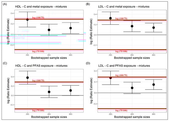
Figure 3. Sufficient sample sizes to estimate the $\delta$-scores in serum lipoprotein-cholesterols at equivalence bounds of $\left[\frac{75}{100},\frac{100}{75}\right]$ with respect to EDC metal mixtures (A,B) and EDC PFAS mixtures (C,D).

5. Concluding Remarks

This paper introduced the idea of the $\delta$-score and sufficient sample size for the exposure–outcome association. $\delta$-score is easily interpretable, scale independent, and because of its connection to Cohen’s $f^2$, it allows for direct comparisons between outcomes measured on different scales, separate studies or in meta-analyses. The $\delta$-score could be used to compare and choose between multiple outcomes with varying units and scales. Furthermore, sample-size determination based on preliminary data might use a sufficient sample size in designing more cost-efficient human studies. We recommend the simultaneous use of the $\delta -$score and regression coefficient-based measures in designing studies to balance precision and utility.

This framework has limitations. The bootstrapped estimation of the $\delta$-score assumed that the original sample was well representative of the true target population. Any estimate of the $\delta$-score, therefore, carried this implicit assumption, but such an assumption is at the core of many statistical analyses, and a well-designed study can ideally resolve such issues or be corrected to be well represented. Oversampling with replacement might cause over-fitting of the data, but splitting the data repeatedly in training and testing under various random seeds can overcome this issue [39]. In addition, this theory is based on the likelihood ratio test of nested models, but future work can extend this framework to strictly non-nested or overlapping models [19]. Although the $\delta$-score was initially developed for nested linear models, its theoretical framework can be extended to non-linear regressions, as well as to non-Gaussian error distributions. For example, ref. [40] studied growth variability in harvested fish populations using a nonlinear mixed effects (NLME) model, developed under a Bayesian approach with non-Gaussian distributions. The $\delta -$score can be used for such a model since it basically requires an estimate of the likelihood ratio test statistics under the null and the alternative hypothesis (see the definition of $f^2$ in generalized linear models). The likelihood ratio statistics for this Bayesian formulation of NLME has often been used in the literature and is readily available through various R functions [41]. Further, in cases of non-Gaussian error distribution, the focus should shift to improving the error variance estimate.

Progress can also be made to estimate the $\delta$-score in a high-dimensional setting, for example, in metabolomic studies ([11,42]). Although concepts rooted in “proportion of the variation” are extensively used in genome-wide association studies, such measures are rarely used in environmental epidemiology or population health studies. This highlights new opportunities for theoretical development and practical implementation in exposomic studies, especially in multi-scale geospatial environmental data, where the integration of multi-source high-dimensional data is not straightforward [43]. In conclusion, quantifying the impact of the exposure–mixture on health using the $\delta -$score could have direct implications for policy decisions and, when used with regression estimates, might prove to be very informative.

References

- Futran Fuhrman, V.; Tal, A.; Arnon, S. Why endocrine disrupting chemicals (edcs) challenge traditional risk assessment and how to respond. J. Hazard. Mater. 2015, 286, 589–611. [Google Scholar] [CrossRef] [PubMed]
- Cano, R.; Pérez, J.L.; Dávila, L.A.; Ortega, A.; Gómez, Y.; Valero-Cedeño, N.J.; Parra, H.; Manzano, A.; Véliz Castro, T.I.; Albornoz, M.P.D.; et al. Role of endocrine-disrupting chemicals in the pathogenesis of non-alcoholic fatty liver disease: A comprehensive review. Int. J. Mol. Sci. 2021, 22, 4807. [Google Scholar] [CrossRef] [PubMed]
- Midya, V.; Colicino, E.; Conti, D.V.; Berhane, K.; Garcia, E.; Stratakis, N.; Andrusaityte, S.; Basagaña, X.; Casas, M.; Fossati, S.; et al. Association of prenatal exposure to endocrine-disrupting chemicals with liver injury in children. JAMA Netw. Open 2022, 5, e2220176. [Google Scholar] [CrossRef] [PubMed]
- Ioannidis, J.P.A.; Greenland, S.; Hlatky, M.A.; Khoury, M.J.; Macleod, M.R.; Moher, D.; Schulz, K.F.; Tibshirani, R. Increasing value and reducing waste in research design, conduct, and analysis. Lancet 2014, 383, 166–175. [Google Scholar] [CrossRef]
- Wasserstein, R.L.; Lazar, N.A. The asa statement on p-values: Context, process, and purpose. Am. Stat. 2016, 70, 129–133. [Google Scholar] [CrossRef]
- Cohen, J. Statistical Power Analysis for the Behavioral Sciences; Lawrence Erlbaum Associates: New York, NY, USA, 1976; pp. 273–403. [Google Scholar]
- Schäfer, T.; Schwarz, M.A. The meaningfulness of effect sizes in psychological research: Differences between sub-disciplines and the impact of potential biases. Front. Psychol. 2019, 10, 813. [Google Scholar] [CrossRef]
- Smithson, M. Confidence Intervals; Number No. 140 in Confidence Intervals; SAGE Publications: Thousand Oaks, CA, USA, 2003. [Google Scholar]
- Grissom, R.; Kim, J. Effect Sizes for Research: A Broad Practical Approach; Lawrence Erlbaum Associates: Mahwah, NJ, USA, 2005. [Google Scholar]
- Yang, J.; Benyamin, B.; McEvoy, B.P.; Gordon, S.; Henders, A.K.; Nyholt, D.R.; Madden, P.A.; Heath, A.C.; Martin, N.G.; Montgomery, G.W.; et al. Common snps explain a large proportion of the heritability for human height. Nat. Genet. 2010, 42, 565–569. [Google Scholar] [CrossRef]
- Joubert, B.R.; Kioumourtzoglou, M.A.; Chamberlain, T.; Chen, H.Y.; Gennings, C.; Turyk, M.E.; Miranda, M.L.; Webster, T.F.; Ensor, K.B.; Dunson, D.B.; et al. Powering research through innovative methods for mixtures in epidemiology (prime) program: Novel and expanded statistical methods. Int. J. Environ. Res. Public Health 2022, 19, 1378. [Google Scholar] [CrossRef]
- Chen, H.Y.; Li, H.; Argos, M.; Persky, V.W.; Turyk, M.E. Statistical methods for assessing the explained variation of a health outcome by a mixture of exposures. Int. J. Environ. Res. Public Health 2022, 19, 2693. [Google Scholar] [CrossRef]
- Wilks, S.S. The large-sample distribution of the likelihood ratio for testing composite hypotheses. Ann. Math. Stat. 1938, 9, 60–62. [Google Scholar] [CrossRef]
- Brown, B.W.; Lovato, J.; Russell, K. Asymptotic power calculations: Description, examples, computer code. Stat. Med. 1999, 18, 3137–3151. [Google Scholar] [CrossRef]
- Selya, A.; Rose, J.; Dierker, L.; Hedeker, D.; Mermelstein, R. A practical guide to calculating cohen’s f2, a measure of local effect size, from proc mixed. Front. Psychol. 2012, 3, 111. [Google Scholar] [CrossRef] [PubMed]
- Akaike, H. Information theory and an extension of the maximum likelihood principle. In Selected Papers of Hirotugu Akaike; Parzen, E., Tanabe, K., Kitagawa, G., Eds.; Springer: New York, NY, USA, 1998; pp. 199–213. [Google Scholar]
- Schwarz, G. Estimating the dimension of a model. Ann. Stat. 1978, 6, 461–464. [Google Scholar] [CrossRef]
- Dziak, J.J.; Coffman, D.L.; Lanza, S.T.; Li, R.; Jermiin, L.S. Sensitivity and specificity of information criteria. Brief. Bioinform. 2019, 21, 553–565. [Google Scholar] [CrossRef]
- Vuong, Q.H. Likelihood ratio tests for model selection and non-nested hypotheses. Econometrica 1989, 57, 307–333. [Google Scholar] [CrossRef]
- Schönbrodt, F.D.; Wagenmakers, E.J.; Zehetleitner, M.; Perugini, M. Sequential hypothesis testing with bayes factors: Efficiently testing mean differences. Psychol. Methods 2017, 22, 322–339. [Google Scholar] [CrossRef]
- Morey, R.D.; Rouder, J.N. Bayes factor approaches for testing interval null hypotheses. Psychol. Methods 2011, 16, 406. [Google Scholar] [CrossRef]
- Kruschke, J.K. Bayesian estimation supersedes the t test. J. Exp. Psychol. Gen. 2013, 142, 573. [Google Scholar] [CrossRef]
- Liao, J.G.; Midya, V.; Berg, A. Connecting and contrasting the bayes factor and a modified rope procedure for testing interval null hypotheses. Am. Stat. 2020, 75, 256–264. [Google Scholar] [CrossRef]
- Midya, V.; Liao, J. Systematic deviation in mean of log bayes factor: Implication and application. Commun. Stat.-Theory Methods 2021, 1–10. [Google Scholar] [CrossRef]
- Schuirmann, D.J. A comparison of the two one-sided tests procedure and the power approach for assessing the equivalence of average bioavailability. J. Pharmacokinet. Biopharm. 1987, 15, 657–680. [Google Scholar] [CrossRef] [PubMed]
- Phillips, K.F. Power of the two one-sided tests procedure in bioequivalence. J. Pharmacokinet. Biopharm. 1990, 18, 137–144. [Google Scholar] [CrossRef] [PubMed]
- Phillips, K.F. Power for testing multiple instances of the two one-sided tests procedure. Int. J. Biostat. 2009, 5, 1–14. [Google Scholar] [CrossRef]
- Long, C.; Chen, W.; Yang, R.; Yao, D. Ratio estimation of the population mean using auxiliary information under the optimal sampling design. Probab. Eng. Inf. Sci. 2022, 36, 449–460. [Google Scholar] [CrossRef]
- Liu, H.S.; Wen, L.L.; Chu, P.L.; Lin, C.Y. Association among total serum isomers of perfluorinated chemicals, glucose homeostasis, lipid profiles, serum protein and metabolic syndrome in adults: Nhanes, 2013–2014. Environ. Pollut. 2018, 232, 73–79. [Google Scholar] [CrossRef]
- Jain, R.B.; Ducatman, A. Associations between lipid/lipoprotein levels and perfluoroalkyl substances among us children aged 6–11 years. Environ. Pollut. 2018, 243, 1–8. [Google Scholar] [CrossRef]
- Meneguzzi, A.; Fava, C.; Castelli, M.; Minuz, P. Exposure to perfluoroalkyl chemicals and cardiovascular disease: Experimental and epidemiological evidence. Front. Endocrinol. 2021, 12, 850. [Google Scholar] [CrossRef]
- Buhari, O.; Dayyab, F.; Igbinoba, O.; Atanda, A.; Medhane, F.; Faillace, R. The association between heavy metal and serum cholesterol levels in the us population: National health and nutrition examination survey 2009–2012. Hum. Exp. Toxicol. 2020, 39, 355–364. [Google Scholar] [CrossRef]
- CDC; NCHS. US National Health and Nutrition Examination Survey Data, 2017–2018. Available online: https://wwwn.cdc.gov/nchs/nhanes/search/datapage.aspx?Component=Laboratory&Cycle=2017-2018 (accessed on 1 September 2022).
- Carrico, C.; Gennings, C.; Wheeler, D.C.; Factor-Litvak, P. Characterization of weighted quantile sum regression for highly correlated data in a risk analysis setting. J. Agric. Biol. Environ. Stat. 2015, 20, 100–120. [Google Scholar] [CrossRef]
- Bobb, J.F.; Valeri, L.; Claus Henn, B.; Christiani, D.C.; Wright, R.O.; Mazumdar, M.; Godleski, J.J.; Coull, B.A. Bayesian kernel machine regression for estimating the health effects of multi-pollutant mixtures. Biostatistics 2014, 16, 493–508. [Google Scholar] [CrossRef]
- Colicino, E.; Pedretti, N.F.; Busgang, S.A.; Gennings, C. Per- and poly-fluoroalkyl substances and bone mineral density. Environ. Epidemiol. 2020, 4, e092. [Google Scholar] [CrossRef] [PubMed]
- Keil, A.P.; Buckley, J.P.; O’Brien, K.M.; Ferguson, K.K.; Zhao, S.; White, A.J. A quantile-based g-computation approach to addressing the effects of exposure mixtures. Environ. Health Perspect. 2020, 128, 047004. [Google Scholar] [CrossRef]
- Gibson, E.A.; Nunez, Y.; Abuawad, A.; Zota, A.R.; Renzetti, S.; Devick, K.L.; Gennings, C.; Goldsmith, J.; Coull, B.A.; Kioumourtzoglou, M.A. An overview of methods to address distinct research questions on environmental mixtures: An application to persistent organic pollutants and leukocyte telomere length. Environ. Health 2019, 18, 76. [Google Scholar] [CrossRef]
- Nunez, Y.; Gibson, E.A.; Tanner, E.M.; Gennings, C.; Coull, B.A.; Goldsmith, J.; Kioumourtzoglou, M.A. Reflection on modern methods: Good practices for applied statistical learning in epidemiology. Int. J. Epidemiol. 2021, 50, 685–693. [Google Scholar] [CrossRef] [PubMed]
- Contreras-Reyes, J.E.; López Quintero, F.O.; Wiff, R. Bayesian modeling of individual growth variability using back-calculation: Application to pink cusk-eel (genypterus blacodes) off chile. Ecol. Model. 2018, 385, 145–153. [Google Scholar] [CrossRef]
- Vincenzi, S.; Mangel, M.; Crivelli, A.J.; Munch, S.; Skaug, H.J. Determining individual variation in growth and its implication for life-history and population processes using the empirical bayes method. PLoS Comput. Biol. 2014, 10, e1003828. [Google Scholar] [CrossRef] [PubMed]
- Maitre, L.; Guimbaud, J.B.; Warembourg, C.; Güil-Oumrait, N.; Marcela Petrone, P.; Chadeau-Hyam, M.; Vrijheid, M.; Gonzalez, J.R.; Basagaña, X. State-of-the-art methods for exposure-health studies: Results from the exposome data challenge event. Environ. Int. 2022, 168, 107422. [Google Scholar] [CrossRef]
- Cui, Y.; Eccles, K.M.; Kwok, R.K.; Joubert, B.R.; Messier, K.P.; Balshaw, D.M. Integrating multiscale geospatial environmental data into large population health studies: Challenges and opportunities. Toxics 2022, 10, 403. [Google Scholar] [CrossRef]
Publisher’s Note: MDPI stays neutral with regard to jurisdictional claims in published maps and institutional affiliations. |
© 2022 by the authors. Licensee MDPI, Basel, Switzerland. This article is an open access article distributed under the terms and conditions of the Creative Commons Attribution (CC BY) license (https://creativecommons.org/licenses/by/4.0/).