Abstract
To understand the nonlinear interaction between unsteady aerodynamic forces and the kinematics of structures, we theoretically and numerically investigated the characteristics of lift coefficients produced by a flapping thin flat plate controlled by the rotation axis position. The flat plate was placed in a 2-D incompressible flow at a very low Reynolds number (Re = 300). We showed that the behavior of the unsteady aerodynamic forces suggests the existence of a limit cycle. In this context, we developed a Reduced Order Model (ROM) by resolving the modified van der Pol oscillator using the Taylor development method and computational fluid dynamics (CFD) solutions. A numerical solution was obtained by integrating the differential equation of the modified van der Pol oscillator using the fourth-order Runge–Kutta method (RK4). The model was validated by comparing this solution with the reformulated equation of the added mass lift coefficient. Using CFD and ROM solutions, we analyzed the dependency of the unsteady lift coefficient generation on the kinematics of the flapping flat plate. We showed that the evolution of the lift coefficient is influenced by the importance of the rotation motion of the Leading Edge (LE) or Trailing Edge (TE), according to the position of the rotation axis. Indeed, when the rotation axis is moved towards the LE, the maximum and the minimum values of the lift coefficient are proportional to the downward and upward motions respectively of the TE and the rotation axis. However, when the rotation axis is moved towards the TE, the maximum and the minimum values of the lift coefficient are proportional to the downward and upward motions respectively of the LE and the rotation axis.
1. Introduction
Symmetry plays a pivotal role in aerodynamics at a low Reynolds number [1,2,3]. In recent years, industry has been involved in the production of biomimicking flying and swimming robots as micro air and underwater vehicles at low Reynolds numbers. An attractive research topic for both the biological and aerodynamic fields is the development of vehicles with flapping wings [4,5,6,7,8,9]. The fluid flowing over these vehicles is very complex because of its nonlinear interaction with the structure. Indeed, at a low Reynolds number, airfoils produce oscillatory lift and thrust. So, a thorough understanding of the unsteady aerodynamics and underlying phenomena are required to design effective control methodologies for these vehicles.
To understand unsteady flow fields, studies on flapping thin-airfoil theory have been previously conducted as seen in the literature [10,11,12]. In order to simplify the analytical formulation of the unsteady flow surrounding flapping wings, researchers separate the total aerodynamic load into many effects, such as the load due to the added-mass effect, the rotation-induced load, the translation-induced load, and the delayed stall/leading edge vortex (LEV) [11,13,14,15]. Various researchers have discussed the added mass effect in the context of the flight of insects [8,16,17,18]. This effect is proportional to the acceleration of the fluid mass around the wing. The instantaneous force caused by the added mass inertia is obtained by deriving the equation modeled by Sedov (1956) [19] acting on a two-dimensional wing. Concerning the rotation-induced load, it has been shown that the fast rotation of the wing during the modification of the flapping leads to the circulation of the flow the opposite way, resulting in an increase in the lift [4]. Ellington (1984) [20] and Fung (1993) [21] investigated the effect of the position of the rotational axis on the amount of circulation and thus on the force produced by a rotating wing. They developed an analytical expression linearly relating the aerodynamic force with the position of the rotational axis. Later, this prediction was confirmed with a series of experiments. Dickinson et al. (1999) [5] measured the total rotational circulation by systematically varying the axis of rotation in which they changed the attachment point of the wing on the flapping apparatus. They showed that when the axis of rotation is moved towards the trailing edge, the rotational circulation decays. Consequently, this last changed its sign at one-fourth of a chord length from the trailing edge of the wing. This result indicates that the rotational circulation provokes the generation of force peaks during stroke reversal. Liu et al. (2015) [22] explored the physical foundations of the unsteady thin-airfoil theory. They developed a simple lift formula containing the vortex lift and the lift associated with the fluid acceleration for the flapping wing. The fluid acceleration term contains the added mass lift and other flow unsteady effects.
Brunton et al. (2013) [23] numerically and experimentally analyzed the dynamics of pitching and plunging airfoils at a low Reynolds number. They developed reduced-order models for the unsteady lift over a range of attack angles. These models were verified by comparing them with measurements using large amplitude maneuvers and frequency response plots. The reduced-order modeling of unsteady flows has an important role which is to represent the dynamical system with a few degrees of freedom and to reduce the complexity of the governing equation such as the Navier–Stokes equations. Functions based on reduced-order modeling are calculated from the flow field data. To form a reduced order model to reduce the nonlinear system significantly, the governing equations can be projected onto these reduced basis functions [24,25]. Hartlen and Currie (1970) [26] founded a limit cycle model based on the Rayleigh oscillator for the flow around a cylinder restrained by springs in the stream-wise direction. Later, Marzouk et al. (2007) [27] used numerical simulations of flow past a stationary circular cylinder to develop a reduced-order model based on the van der Pol oscillator for the lift and drag coefficients. They proved that this model matched the numerical simulation results in the time and the spectral domains. Akhtar et al. (2009) [28] modeled lift and drag coefficients of flow past elliptic cylinders with a generalized van der Pol–Duffing oscillator. Recently, Venkataraman et al. (2014) [29] studied the existence condition of the limit cycle for the modified van der Pol oscillator. By using the multiple scales method, they obtained a minimal model for vortex-shedding from an aerofoil with a porous coating of flow-compliant feather-like actuators. They noticed that this model helps understand the passive achievement of flow control. Khalid et al. (2017) [30] revealed that aerodynamic forces produced by oscillating NACA-0012 airfoils are independent of the initial kinematic conditions suggesting the existence of a limit cycle. Using numerical simulations, they analyzed the shedding frequencies close to the excitation frequencies and modeled the unsteady lift force with a modified van der Pol oscillator. The frequencies and the damping terms in the reduced-order model (ROM) were estimated using the multiple scales method and steady-state spectral analysis for computational fluid dynamics (CFD) solutions. Hafien et al. (2019) [31] developed a reduced order model for the lift coefficient of an airfoil equipped with extrados and/or trailing edge flexible flaps at low Reynolds number. This model was obtained by resolving the modified van der Pol oscillator using the Taylor development method.
In this research, we studied unsteady flow around a flapping flat plate at a very low Reynolds number (Re = 300). First, we developed a reduced order model (ROM) of the lift coefficient based on the modified van der Pol oscillator. Then, we reformulated the equation of the added mass lift coefficient to conform it to this oscillator model. The new form of the added mass lift coefficient was used to validate the ROM by resolving the differential equation of the modified van der Pol oscillator by using the Runge-Kutta (RK4) method. For the total lift coefficient, the parameters of the model were obtained by using the Taylor development method and computational fluid dynamics (CFD) solutions. Finally, we used the ROM and CFD results to study and analyze the effect of modifying the rotation axis of the flapping flat-plate on vortex-shedding, and therefore on the unsteady lift coefficient.
2. Reduced-Order Model
The behavior of a nonlinear system is characterized as a limit cycle when the response of this system limits itself to a periodic, a quasiperiodic, or a chaotic attractor. This phenomenon appears under the effect of an energy dissipation mechanism, which represents a closed trajectory in the phase space [32]. Khalid et al. (2017) [30] tested the oscillating airfoil lift for various initial conditions. They showed that the initial kinematic states do not have an effect on the dynamic system. This proves that the unsteady aerodynamic coefficients of an oscillating airfoil describe the behavior of a limit cycle. Researchers have previously concluded that the van der Pol oscillator is the more accurate representation of the lift coefficient [33].
The general form of the van der Paul oscillator is described as [34]:
where c, αi, and βi are the coefficient of linear damping, the coefficients of quadratic nonlinear terms, and the coefficients of cubic nonlinear terms, respectively.
Venkataraman (2013) [35] studied the condition of existence of the limit cycle for the general van der Pol oscillator. He showed that this oscillator can define the lift coefficient oscillation, which is characterized by a limit cycle when: α1 = 0, α2 = 0, α3 = 1, β2 = 0, and β4 = −1, see Table 1.

Table 1.
Dependence of limit cycle existence on the nonlinearities in Equation (1) [35].
Consequently, the van der Pol oscillator can be written as [35]:
where w, μ, β, and α are the parameters of the modified van der Pol oscillator.
By using the Taylor development method, resolving the modified van der Pol oscillator shows that: y = γ1exp(−iwt) + γ2exp(iwt), y = ∂x/∂t, see detail in [31]. Hence, by using the particular solutions y = γs·sin(wt)+ γc·cos(wt) and x = Cl − (Cl is the lift coefficient) in Equation (2), we show that:
where
and
Replacing sini(wt)·cosj(wt) (i, j = 0, 1, 2, 3; 1 < i + j ≤ 3) with their expressions as a function of sin(nwt) and/or cos(nwt) (n = 0,1, 2, 3), we show that:
where
and
3. ROM for the Added Mass Lift Coefficient (Clma)
Analytical modeling of aerodynamic efforts of oscillating airfoils can be classified into three groups: steady state models, quasi-steady models and unsteady models. Due to the difficulties of modeling unsteady aerodynamic forces in a single term, researchers developed quasi-steady models which separate these forces into many parts. von Kármán and Sears (1938) [36] expressed, in one of the first studies, the unsteady lift as a sum of the quasi-steady Kutta–Joukowski lift, the added-mass lift, and the wake-induced contribution. Later, based on experimental, computational and theoretical studies, researchers showed that the lift in flapping wings was improved by various mechanisms such as the Weis-Fogh’s “clap and fling” mechanism [37], the delayed stall/leading edge vortex (LEV) [7], the added mass effect [18,19], the Kramer effect/rotational lift [8,38], etc. Recently, Wang et al. (2016) [39] proposed a quasi-steady model that included four aerodynamic loading terms for a flapping wing lift: translation load, rotation load, coupling (translation + rotation) load, and the added-mass effect. In this section, we show that the added mass lift coefficient (Clma) can be reformulated in order to conform Equation (5) to exhibit a behavior similar to the reduced order model based on the modefied van der Pol oscillator (2). This helps to analyze and understand the underlying physics of the nonlinear system for total lift.
We consider a flapping thin flat plate with a chord c, placed in the flow field with free stream velocity U∞ at a very low Reynolds number (Re = 300). The kinematics of the two-dimensional flat plate is defined as (see Figure 1):
where θ(t), θm, and θ0 are the instantaneous angle of attack (AOA), the time-averaged AOA, and the pitching amplitude, respectively. z(t) and z0 are the instantaneous vertical position of the center of the plate and the heaving amplitude. w = 2πf (f = 1/T is the flapping frequency).
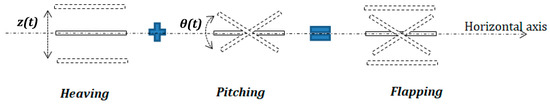
Figure 1.
Schematic of flapping flat plate kinematics.
Using the equation expressed by Seldov (1965) [19] for the aerodynamic force due to the added mass effect of a thin airfoil, we show that Clma can be written as:
where
and
The added mass force has a significant contribution to the total aerodynamic force of the flapping wings during and near the stroke reversals [10]. Researchers show that the added mass is dependent on this frequency and amplitude of flapping wings [40].
3.1. Reformulation of the Clma Equation
For a low angle of attack θ, can be writen as a function of and , as shown here (see Appendix B):
where
Using Equation (8), we show that:
Introducing Equations (10) and (11) into Equation (7), we have:
where
Finally, we obtain a new form of Clma identical to Equation (5) that was obtained by resolving the van der Pol oscillator model (2):
where
Table 2 shows the parameters of Equations (12) and (13) that describe the added mass lift coefficient (Clma(t)) after reformulation in the case of St = fc/U∞ = 0.6; θm = 10°; θ0 = 30°; and z0 = 0.25c (these values will be used for the continuation of this work). It is clear that the approached form of Clma(t) defined in Equation (13) agrees well with the exact form of Equation (7) (see Figure 2).
Table 2.
Parameters of Equations (12) and (13) for St = fc/U∞ = 0.6; θm = 10°; θ0 = 30°; and z0 = 0.25c.
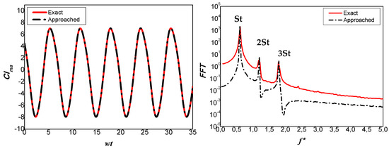
Figure 2.
Comparison between the approached (12) and the exact (7) forms of the added mass lift coefficient for St = fc/U∞ = 0.6; θm = 10°; θ0 = 30°; and z0 = 0.25c: evolution of the lift coefficient as a function of wt (left) and FFT Power Spectral Density of the lift coefficient as a function of the dimensionless frequency f* = c/U∞t (right).
3.2. Validation of the ROM with the RK4 Method
In order to validate the proposed reduced order model, we used the fourth-order Runge–Kutta method (RK4) to numerically integrate the modified van der Pol oscillator (12). This solution is verified for the particular case; the added mass lift coefficient for St = 0.6; θm = 10°; θ0 = 30°; and z0 = 0.25c.
Now, by putting the ordinary differential Equation (2) in the vector , we obtain:
Using the Runge-Kutta-4 method, we have:
where for n = 1, 2, 3, …
Using Equation (14) we show that:
So, finally we obtain:
We replace x and y by Cl and ∂Cl/∂t respectively to determine the lift coefficient time histories of the oscillating flat plate. To determine the linear damping, the quadratic nonlinear and the cubic nonlinear coefficients of the modified van der Pol oscillator (μ, β, and α), we introduce the analytical expression of the lift coefficient (4) into the differential Equation (2):
where Cl, ∂Cl/∂t, and ∂2Cl/∂t2 are:
Moreover, we calculate (∂Cl/∂t)2 and (∂Cl/∂t)3 and neglect the amplitude proportional to the frequencies nw when n > 3. We show that:
where
For the lift coefficient generated with added mass, we show that μ = 0.604, β = −0.0116, and α = 0.00159. The initial conditions Cl(0) and Cl’(0) were calculated from the analytical expression of the added mass lift coefficient (12). By using these values in equation system (21), the Runge-Kutta-4 method allows us to determine the time history of Clma. The comparison between the analytical expression (12) and the solution obtained by resolution of the van der Pol oscillator model using the Runge-Kutta-4 method (ROM R-K4) shows the validation of the proposed reduced order model (see Figure 3).
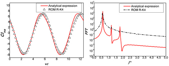
Figure 3.
Comparison of the solutions from analytical expression (12) and the ROM R-K4: evolution of the lift coefficient as a function of wt (left) and FFT Power Spectral Density of the lift coefficient as a function of the dimensionless frequency f* = c/U∞t (right).
4. CFD Study
The use of a computational tool helps to quickly estimate the response of the physical part of nonlinear systems. In this section we employed the data obtained from numerical simulations using ANSYS-Fluent in order to calculate the proposed reduced-order model parameters. The CFD solver and the analytical solution of the van der Pol equation were used as the first step towards the development of the reduced-order models for the total lift coefficient of the flapping flat plate.
4.1. Numerical Model
We considered a thin flat plate with a chord c placed in the flow field at a Reynolds number equal to 300. To avoid the effect of disturbances on the boundaries, the radius of the C-type domain was kept at 12.5c, so, the computational domain consisted of 12.5c, at: the top, bottom, upstream, and downstream of the flapping flat plate, see Figure 4.
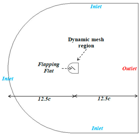
Figure 4.
Boundary conditions of the computational domain.
The flow past the flapping flat plate is simulated by solving the 2D incompressible Navier–Stokes equations using the finite volume method. The differential form of the conservation equations of mass and momentum are [ANSYS-Fluent]:
where ui is the velocity, p is the pressure, ρ is the fluid density, and υ is the kinematic viscosity of the fluid.
A second-order upwind scheme is employed for the spatial discretization of the convection terms of the transport equations. A second-order implicit method is used to approximate the temporal discretization of the governing equations. The algorithm of the pressure–velocity coupling used is “PISO”. An irregular grid was used for the computational domain. We employed 300 nodes around the flat plate and 19,138 cells in the domain. In the region near the moving flat plate, we used dynamic mesh techniques (Remeshing and Smoothing methods) to accord the instantaneous position of the plate. The kinematics of the latter is defined by a user-defined function (UDF) written in C-language and coupled with the Fluent-Macros. As mentioned in the last section (§3.1), the instantaneous AOA and the instantaneous vertical position of the axis of rotation are:
4.2. Validation of the CFD Results
We conducted a test series to verify and validate the numerical results obtained from the computational model. First, we verified the independence between the numerical solution and the time-step size as well as the mesh refinement. After that, the present results were validated with the computational results of other researchers.
Concerning the verification of the numerical solver focused on its self-consistency, three different levels of time step size dt and grid refinement were tested for six distinct cases. For T = 200dt, we used three grids: grid 1 with 16,560 cells (200 nodes around the flat plate), grid 2 with 19,138 cells (300 nodes around the flat plate), and grid 3 with 21,700 cells (400 nodes around the flat plate). Next, using grid 2, we tested three time step sizes: dt1 = T/100, dt2 = T/200, and dt3 = T/400. Figure 5a,b shows the evolution of the lift coefficient as a function of the dimensionless time t/T for the different tested cases. It is clear that the simulation results were not significantly affected by the grid refinement and time step size. Grid 2 and dt2 yielded a stable solution and will be used in the continuation of this paper. In order to validate our computational model, we compared the time history of the present lift coefficient computed using CFD-Fluent with those obtained by Liu et al. (2015). We noted that the lift coefficient oscillation was independent of the initial conditions. Good agreement was obtained between the present results and the results from the literature for St = 0.06 and St = 0.6, see Figure 5c,d.
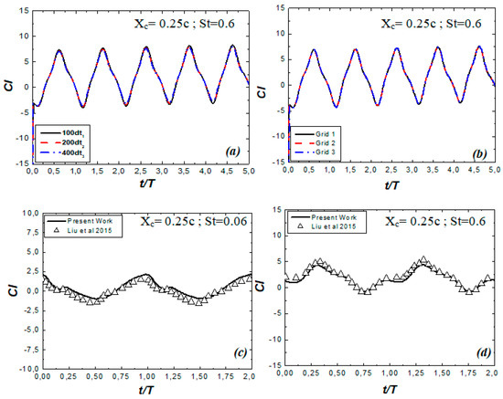
Figure 5.
Validation of the present computational model. Time history of the lift coefficient for: (a) different time step sizes and (b) different mesh refinement; (c,d) comparison of the present results with the literature results [22]. The axis of rotation of the flapping flat plate is placed at one-fourth of the chord from the leading edge (Xc = 0.25c).
4.3. Results and Discussion
To validate the proposed reduced order model, we compared the lift solution of the van der Pol oscillator model with those from the CFD. We studied temporal profiles and the harmonics in the spectra of the unsteady lift for three different rotation axis positions: Xc = 0.25c; Xc = 0.425c, and Xc = 0.65c (see Figure 6). It is clear that the ROM does not only accurately capture the numerical simulation results in the time domain but also in the spectral domain. The curves obtained from the spectral analysis show that the amplitudes that were proportional to the frequencies nSt when n > 3 were neglected in the ROM compared to the CFD model. Table 3 shows the constant parameters of Equation (18) obtained from the modified van der Pol oscillator model for the lift coefficient in all the studied cases. We notice that the mean value of the lift coefficient Cl0 increased when the rotation axis gets closer to the leading edge. However, the amplitudes A1, A2, and A3 increased when the rotation axis moved away from the middle of the flat. The ROM and the CFD model enabled us to determine the phases which were proportional to the main, second, and third Strouhal numbers (ϕ1, ϕ2, and ϕ3) for each position of the rotation axis: ϕi(0.25) < ϕi(0.425) < ϕi(0.65).
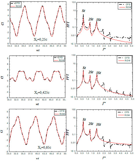
Figure 6.
Comparison of the results from the ROM and the CFD model for three different rotation axis positions. Ocillating lift coefficient in the time domain (left) and in the frequency domain (right).
Table 3.
Parameters of Equations (18) for: Xc = 0.25c; Xc = 0.425c; and Xc = 0.65c.
For Xc = 0.25c, the speed of the trailing Edge (TE) is more important than the Leading Edge (LE). For this reason, the minimum value of the lift coefficient (Clmin) is proportional to the upward motion of the TE and the rotation axis of the flat plate. However, the maximum value Clmax is proportional to their downward motion (see Figure 7). Conversely, the speed of the TE is less important compared to the LE for Xc = 0.65c. Consequently, Clmin and Clmax are proportional to the upward and downward motions, respectively, of the LE and the rotation axis of the flat plate (see Figure 7). This explains the difference between the phases ϕ1(0.25) = π + 0.798 and ϕ1(0.65) = 2π + 0.2153 (see Table 3). Concerning the case where Xc = 0.425c, it can be seen from Figure 7 that the lift coefficient has two maximum and two minimum values during each oscillation cycle. On the one hand, Clmin1(t/T = 0.11) and Clmax2(t/T = 0.55) are proportional to the upward and downward motions, respectively, of the TE and the rotation axis of the flat plate. On the other hand, Clmax1(t/T = 0.38) and Clmin2(t/T = 0.83) are proportional to the downward and upward motions, respectively, of the LE and the rotation axis. This proves for the case where Xc = 0.425c that the movements of the LE and the TE have the same effect on the lift coefficient evolution due to the close distance between the rotation axis and the middle of the flat plate.
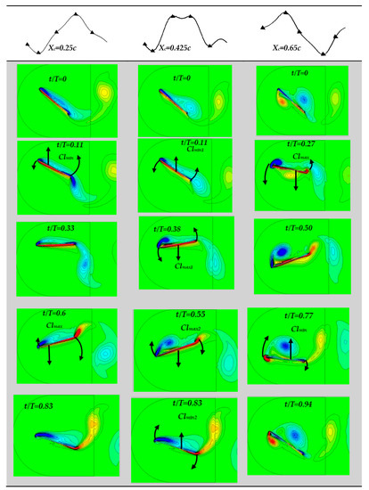
Figure 7.
Instantaneous vorticity contours (contour levels varying from −22 to 22) during each oscillation cycle for different rotation axis positions: Xc = 0.25c; Xc = 0.425c, and Xc = 0.65c. Dependency between the unsteady lift coefficient and the flow topology.
A reverse von Karman Vortex Street is produced in the wake during the oscillation of the thin-airfoil. This leads to the generation of periodic aerodynamic forces in nature including several harmonics of the vortex shedding frequency. Consequently, the modification of the lift coefficient characteristic is caused by the modification of the flow topology. When the flat plate oscillates, a von-Karman vortex street (clockwise rotating vortices) or reverse von-Karman Vortex Street (counterclockwise rotating vortices) is generated in the wake. The instability in the boundary layer forms the Leading Edge Vortices (LEV).
These vortices move downstream and detach from the flat plate before reaching the Trailing Edge (TE), see Figure 7. Depending on the rotation axis position, which affects the kinematics of the flapping flat plate, the Leading Edge and Trailing Edge vortices (LEV and TEV) interact in the wake. It is clear that when the rotation axis nears the leading edge (Xc = 0.25c), stronger TEVs were produced. However, as shown in Figure 7, when the rotation axis nears the trailing edge (Xc = 0.65c), the stronger LEVs appear in both the extrados and intrados of the flat plate. As a result, the couples of the counter-rotating vortices, LEV and TEV, are close to each other in the wake region behind the flapping flat plate for Xc = 0.65c. However, for the Xc = 0.25c case, the vortices push away from each other, see Figure 8.
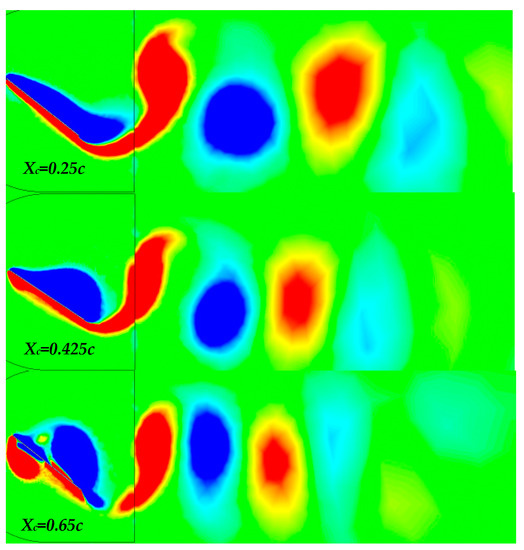
Figure 8.
Contours of the instantaneous vorticity-field (dimensionless velocity-Curl w.c/U varying between −2.2 and 2.2) in the wake region behind the flapping flat plate for different rotation axis positions: Xc = 0.25c; Xc = 0.425c and Xc = 0.65c.
This modification in the flow topology leads to: the decrease in the mean lift coefficient when the rotation axis is further away from the leading edge; the increase in the oscillation amplitudes, Ai, of the unsteady lift coefficient when the rotation axis is further away from the middle of the flat plate; the modification of the phases, ϕi, as a function of the importance of the rotation speed of the TE or LE.
5. Conclusions
In this paper we have studied the 2D incompressible flow at Reynolds number Re = 300 and Strouhal number St = 0.6 past a flapping flat plate. Three kinematic cases were studied: flapping flat plate with rotation axis positions: Xc = 0.25c, Xc = 0.425c, and Xc = 0.65c. We developed a Reduced Order Model based on the modified van der Pol oscillator to characterize the behavior of the nonlinear unsteadiness of the lift coefficient as a limit cycle. The equation of the added mass lift coefficient was reformulated to exhibit the reduced order model (ROM). Using the fourth-order Runge–Kutta method (RK4) we numerically integrated the differential equation of the modified van der Pol oscillator. Good agreement was obtained between this solution and the reformulated equation of the added mass lift coefficient. For the total lift coefficients, the results obtained from the ROM agree well with those obtained from the CFD both in the temporal and spectral domains. The modification of the rotation axis position, which affects the rotation speed of the Leading Edge and the Trailing Edge of the flat plate, leads to the modification of the flow topology as well as the characteristics of the unsteady aerodynamic forces. Based on the CFD and ROM solutions we showed that: the mean lift coefficient decreases when the rotation axis moves further away from the leading edge; the oscillation amplitudes, Ai, of the unsteady lift coefficient increase when the rotation axis moves further away from the middle of the flat plate; and the phases, ϕi, are modified proportionally to the importance of the rotation speed of the TE or LE.
Author Contributions
Conceptualization, C.H.; methodology, C.H.; software, C.H.; validation, C.H. and A.M.; formal analysis, C.H. and A.M.; investigation, C.H. and A.M.; resources, C.H.; data curation, C.H.; writing—original draft preparation, C.H.; writing—review and editing, C.H. and A.M.; visualization, C.H. and A.M.; supervision, C.H. and A.M.; project administration, C.H. and A.M.; funding acquisition, C.H. All authors have read and agreed to the published version of the manuscript.
Funding
This research received no external funding.
Data Availability Statement
The authors are grateful to anonymous reviewers for helpful comments and suggestions that helped us to improve the paper.
Conflicts of Interest
The authors declare no conflict of interest.
Appendix A
We consider the equation:
where x is the variable term and Ac, As, A, and ϕ are constant parameters.
At x = xm, A·sin(xm + ϕ) achieves its maximum (or minimum) value, thus:
So
where n = 0, 1, 2, 3, …
Finally by replacing x by xm = Atg(As/Ac) in (A1) we obtain:
Appendix B
Defining the function :
Using the Taylor development, we have:
Replacing cos2(x) by 0.5(1 + cos(2x)), we obtain:
where
We know that:
and
Thus, we can obtain the solution with error estimation :
where
and the error estimations
This error is negligible for low angles θm and θ0. In Figure A1, we display the error estimations and for x = 0, θm = 10° θ0 = 30° and n varying between 0 and 20.
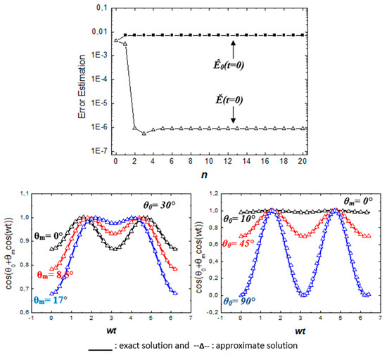
Figure A1.
Error estimations and for x = 0, θm = 10° θ0 = 30° and n varying between 0 and 20.
References
- Hafien, C.; Bourehla, A.; Bouzayane, M. Passive Separation Control on a Symmetric Airfoil via Elastic-Layer. J. Appl. Fluid Mech. 2016, 9, 2569–2580. [Google Scholar] [CrossRef]
- Rodriguez-Eguia, I.; Errasti, I.; Fernandez-Gamiz, U.; Blanco, J.M.; Zulueta, E.; Saenz-Aguirre, A.A. A Parametric Study of Trailing Edge Flap Implementation on Three Different Airfoils Through an Artificial Neuronal Network. Symmetry 2020, 12, 828. [Google Scholar] [CrossRef]
- Stevens, P.R.R.J.; Babinsky, H.; Manar, F.; Mancini, P.; Jones, A.R.; Nakata, T.; Phillips, N.; Bomphrey, R.J.; Gozukara, A.C.; Granlund, K.O.; et al. Experiments and Computations on the Lift of Accelerating Flat Plates at Incidence. AIAA J. 2017, 55, 3255–3265. [Google Scholar] [CrossRef]
- Chen, Y.H.; Skote, M. Study of lift enhancing mechanisms via comparison of two distinct flapping patterns in the dragonfly Sympetrum flaveolum. Phys. Fluids 2015, 27, 033604. [Google Scholar] [CrossRef]
- Dickinson, M.H.; Lehmann, F.O.; Sane, S.P. Wing Rotation and the Aerodynamic Basis of Insect Flight. Science 1999, 284, 1954–1960. [Google Scholar] [CrossRef] [PubMed]
- Ho, S.; Nassef, H.; Pornsinsirirak, N.; Tai, Y.C.; Ho, C.M. Unsteady aerodynamics and flow control for flapping wing flyers. Prog. Aerosp. Sci. 2003, 39, 635–681. [Google Scholar] [CrossRef]
- Maybury, W.J.; Lehmann, F.O. The fluid dynamics of flight control by kinematic phase lag variation between two robotic insect wings. J. Exp. Biol. 2004, 207, 4707–4726. [Google Scholar] [CrossRef] [PubMed] [Green Version]
- Sane, S.P.; Dickinson, M.H. The aerodynamic effects of wing rotation and a revised quasi-steady model of flapping flight. J. Exp. Biol. 2002, 205, 1087–1096. [Google Scholar] [CrossRef] [PubMed]
- Yang, L.J.; Hsiao, F.Y.; Tang, W.T.; Huang, I.C. 3D Flapping Trajectory of a Micro-Air-Vehicle and its Application to Unsteady Flow Simulation. Int. J. Adv. Robot. Syst. 2013, 10, 264. [Google Scholar] [CrossRef]
- Liu, L.; Sun, M. The added mass forces in insect flapping wings. J. Theor. Biol. 2018, 437, 45–50. [Google Scholar] [CrossRef] [PubMed]
- Wang, S.; Zhang, X.; Guowei, H.; Tianshu, L. A lift formula applied to low-Reynolds-number unsteady flows. Phys. Fluids 2013, 25, 093605. [Google Scholar] [CrossRef] [Green Version]
- Xu, M.; Wei, M.; Yang, T.; Lee, Y.S. An embedded boundary approach for the simulation of a flexible flapping wing at different density ratio. Eur. J. Mech. B/Fluids 2016, 55, 146–156. [Google Scholar] [CrossRef]
- Berman, G.J.; Wang, Z.J. Energy-minimizing kinematics in hovering insect flight. J. Fluid Mech. 2007, 582, 153–168. [Google Scholar] [CrossRef] [Green Version]
- Ellington, C.P.; Van den Berg, C.; Willmott, A.P.; Thomas, A.L.R. Leading-edge vortices in insect flight. Nature 1996, 384, 626–630. [Google Scholar] [CrossRef]
- Whitney, J.P.; Wood, R.J. Aeromechanics of passive rotation in flapping flight. J. Fluid Mech. 2010, 660, 197–220. [Google Scholar] [CrossRef] [Green Version]
- Minotti, F.O. Unsteady two-dimensional theory of a flapping wing. Phys. Rev. E 2002, 66, 051907. [Google Scholar] [CrossRef]
- Sunada, S.; Kawachi, K.; Matsumoto, A.; Sakaguchi, A. Unsteady forces on a two-dimensional wing in plunging and pitching motions. AIAA J. 2001, 39, 1230–1239. [Google Scholar] [CrossRef]
- Zbikowski, R. On aerodynamic modelling of an insect-like flapping wing in hover for micro air vehicles. Philos. Trans. R. Soc. A 2002, 360, 273–290. [Google Scholar] [CrossRef] [PubMed]
- Sedov, L.I. Two-Dimensional Problems in Fuild Dynamics and Aero-Dynamics; Interscience: New York, NY, USA, 1965; pp. 20–30. [Google Scholar]
- Ellington, C.P. The aerodynamics of hovering insect flight. IV. aerodynamic mechanisms. Philos. Trans. R. Soc. B Biol. Sci. 1984, 305, 79–113. [Google Scholar]
- Fung, Y.C. An Introduction to the Theory of Aeroelasticity; Dover: New York, NY, USA, 1993. [Google Scholar]
- Liu, T.; Wang, S.; Zhang, X.; He, G. Unsteady Thin-Airfoil Theory Revisited: Application of a Simple Lift Formula. AIAA J. 2015, 53, 1492–1502. [Google Scholar] [CrossRef]
- Brunton, S.; Rowley, C.W.; Williams, D. Reduced-order unsteady aerodynamic models at low Reynolds numbers. J. Fluid Mech. 2013, 724, 203–233. [Google Scholar] [CrossRef]
- Akhtar, I.; Borggaard, J.; Hay, A. Shape Sensitivity Analysis in Flow Models Using a Finite-Difference Approach. Math. Probl. Eng. 2010, 2010, 209780. [Google Scholar] [CrossRef] [Green Version]
- Sirovich, L. Turbulence and the Dynamics of Coherent Structures. Q. Appl. Math. 1987, 45, 561–571. [Google Scholar] [CrossRef] [Green Version]
- Hartlen, R.; Currie, I. Lift-oscillator model of vortex-induced vibration. J. Eng. Mech. Div. 1970, 96, 577–591. [Google Scholar] [CrossRef]
- Marzouk, O.A.; Nayfeh, A.H.; Akhtar, I.; Arafat, H.N. Modeling Steady-State and Transient Forces on a Cylinder. J. Vib. Control 2007, 13, 1065–1091. [Google Scholar] [CrossRef] [Green Version]
- Akhtar, I.; Marzouk, O.A.; Nayfeh, A.H. A van der Pol–Duffing Oscillator Model of Hydrodynamic Forces on Canonical Structures. J. Comput. Nonlinear Dyn. 2009, 4, 041006. [Google Scholar] [CrossRef]
- Venkataraman, D.; Bottaro, A.; Govindarajan, R. A minimal model for flow control on an aerofoil using a poro-elastic coating. J. Fluids Struct. 2014, 47, 150–164. [Google Scholar] [CrossRef]
- Khalid, M.S.U.; Akhtar, I. Nonlinear Reduced-Order Models for Aerodynamic Lift of Oscillating Airfoils. J. Comput. Nonlinear Dyn. 2017, 12, 051019. [Google Scholar] [CrossRef]
- Hafien, C.; Ben Mbarek, T. Reduce d order model for the lift coefficient of an airfoil equipped with extrados and/or trailing edge flexible flaps. Comput. Fluids 2019, 180, 82–95. [Google Scholar] [CrossRef]
- Moon, F.C. Applied Dynamics: With Applications to Multibody and Mechatronic Systems; Wiley: Hoboken, NJ, USA, 1998. [Google Scholar]
- Nayfeh, A.H.; Owis, F.; Hajj, M.R. A model for the coupled lift and drag on a circular cylinder. In Proceedings of the DETC03, ASME 2003 Design Engineering Technical Conferences and Computers and Information in Engineering Conference, Chicago, IL, USA, 2–6 September 2003. [Google Scholar]
- Richard, H. Rand Lecture Notes on Nonlinear Vibrations; Department of Theoretical and Applied Mechanics, Cornell University: Ithaca, NY, USA, 2005. [Google Scholar]
- Venkataraman, D. Flow Control Using a Porous, Compliant Coating of Feather-like Actuators. Ph.D. Thesis, Department of Civil, Chemical and Environmental Engineering, University of Genova, Genoa, Italy, 19 March 2013. [Google Scholar]
- von Kármán, T.; Sears, W.R. Airfoil Theory for Non-Uniform Motion. J. Aeronaut. Sci. 1938, 5, 379–390. [Google Scholar] [CrossRef]
- Weis-Fogh, T. Quick estimates of flight fitness in hovering animals, including novel mechanisms for lift production. J. Exp. Biol. 1973, 59, 169–230. [Google Scholar] [CrossRef]
- Sane, S.P.; Dickinson, M.H. The control of flight force by a flapping wing: Lift and drag production. J. Exp. Biol. 2001, 204, 2607–2626. [Google Scholar] [CrossRef] [PubMed]
- Wang, Q.; Goosen, H.; van Keulen, F. A predictive quasi-steady model of aerodynamic loads on flapping wings. J. Fluid Mech. 2016, 800, 688–719. [Google Scholar] [CrossRef] [Green Version]
- Zakaria, M.Y.; Pereira, D.A.; Ragab, S.A.; Hajj, M.R.; Marques, F.D. An Experimental Study of Added Mass on a Plunging Airfoil Oscillating with High Frequencies at High Angles of Attack. In Proceedings of the 33rd AIAA Applied Aerodynamics Conference, Dallas, TX, USA, 22–26 June 2015. [Google Scholar] [CrossRef]
Publisher’s Note: MDPI stays neutral with regard to jurisdictional claims in published maps and institutional affiliations. |
© 2022 by the authors. Licensee MDPI, Basel, Switzerland. This article is an open access article distributed under the terms and conditions of the Creative Commons Attribution (CC BY) license (https://creativecommons.org/licenses/by/4.0/).