High-Dimensional Conditional Covariance Matrices Estimation Using a Factor-GARCH Model

Abstract

Estimation of a conditional covariance matrix is an interesting and important research topic in statistics and econometrics. However, modelling ultra-high dimensional dynamic (conditional) covariance structures is known to suffer from the curse of dimensionality or the problem of singularity. To partially solve this problem, this paper establishes a model by combining the ideas of a factor model and a symmetric GARCH model to describe the dynamics of a high-dimensional conditional covariance matrix. Quasi maximum likelihood estimation (QMLE) and least square estimation (LSE) methods are used to estimate the parameters in the model, and the plug-in method is introduced to obtain the estimation of conditional covariance matrix. Asymptotic properties are established for the proposed method, and simulation studies are given to demonstrate its performance. A financial application is presented to support the methodology.

1. Introduction

Estimation of a conditional covariance matrix is an important and popular topic in statistics and econometrics with wide applications in many disciplines, such as engineering, environmentology, psychology, economics and finance. A traditional approach to estimating conditional covariance matrices is based on multivariate GARCH models, e.g., the vectorized multivariate GARCH (VEC-GARCH) model of [1], the Baba, Engle, Kraft and Krone GARCH (BEKK-GARCH) model of [2], the constant conditional correlation GARCH (CCC-GARCH) model of [3] and the dynamic conditional correlation GARCH (DCC-GARCH) model of [4].

These GARCH models can be called symmetric GARCH models, which assume that the response of conditional covariance (volatility) to a shock is a function of the shock strength only without any correlation with the sign of the shock. To capture the leverage effects, some multivariate GARCH models take into account negative shocks with a larger impact on their conditional covariance compared with positive shocks of the same absolute value.

That is to say, the new impact curve, which traces the relation between conditional covariance and the previous shock, is asymmetric. These asymmetric multivariate GARCH models include the asymmetric dynamic covariance GARCH (ADC-GARCH) model of [5], the generalized diagonal VEC-GARCH model of [6] and related models of [7,8].

However, common multivariate GARCH models cannot be directly applied to ultra-high dimensional data, which is often the case when constructing a portfolio allocation in finance. This is because there are too many parameters to be estimated when the dimension is large, see, e.g., [9]. To overcome the problems caused by high dimensions, various methods have been developed to reduce the dimension of data and the number of parameters.

One of effective methods for dimension reduction is the factor analysis for time series, see [10,11,12,13,14] focusing on the conditional mean and [15,16,17] focusing on the conditional covariance. In addition, there are some variants of the factor model that introduce the GARCH structure to describe the conditional covariance, e.g., the full-factor multivariate GARCH (FF-GARCH) model introduced by [18], the orthogonal GARCH (O-GARCH) model proposed by [19] and the generalized O-GARCH (GO-GARCH) model of [20].

Ref. [21] investigated the asymptotic theory for the general factor GARCH model that nested the above three models. But the model proposed by [21] can’t reduce the dimension if loading matrix is a square matrix. O-GARCH model as a special case of [21] is a successful multivariate GARCH model with a parsimonious form. This not only captures the dynamics of conditional covariance but can also reduce the dimensions effectively if the model is identified fairly.

However, the O-GARCH model treats all principal components as conditionally uncorrelated random variables, which may lead to a miss-specification and non-negligible errors in the fitting (see [22]). Moreover, when the number of factors is smaller than the dimension, the conditional covariance matrix obtained by the factor GARCH model is only non-negative definite but not positive-definite.

Recently, Ref. [23] proposed a dynamic structure and developed an estimation procedure for high-dimensional conditional covariance matrices. Their work is insightful but not applicable for the cases when the dimension p is equal to or larger than the sample size T. However, in practical applications, there are many cases facing $p>T$ when modelling the conditional covariance matrices. Hence, it makes sense to study the issue under ultra-high dimensional cases.

Motivated by the above literature, we propose an alternative model for estimating high-dimension conditional covariance matrix. The basic idea is to use a factor model to reduce the dimensions first, then fit the low-dimensional CCC-GARCH model to the common factor and use the univariate GARCH model to fit the idiosyncratic components.

The rest of the article is organised as follows. We begin in Section 2 with the proposed model, estimation methodology and the modelling procedure. In Section 3, asymptotic properties of the proposed estimators, including the necessary assumptions, are given. Section 4 constructs a portfolio allocation based on the formula for Markowitz’s optimal portfolio using the proposed model as a conditional covariance matrix. To assess the performance of the proposed method, we illustrate simulation and a real example in Section 5. Section 6 provides our conclusions. All proofs of theoretical results are put in the Appendix A.

Throughout the paper, we use $A^{\tau }$, ${\lambda }_{\min }\left(A\right)$ and ${\lambda }_{\max }\left(A\right)$ to denote the transpose and the minimum and maximum eigenvalues of a matrix A. Let $\mathrm{vec}\left(A\right)$ be the column-stacking vector of a matrix A. The notations ${\Vert A\Vert }_F$, $\Vert A\Vert$ and ${\Vert A\Vert }_{\max }$ represent the Frobenius norm, spectral norm (operator norm) and element-wise norm of a matrix A, defined respectively by ${\Vert A\Vert }_F={\mathrm{tr}}^{1/2}\left(A^{\tau }A\right)$, $\Vert A\Vert =\lambda {}_{\max }^{1/2}\left(A^{\tau }A\right)$ and ${\Vert A\Vert }_{\max }={max}_{i,j}|a_{ij}|$.

When A is a vector, both ${\Vert A\Vert }_F$ and $\Vert A\Vert$ are equal to the Euclidean norm. For a random sequence $a_n$, $a_n=O_p\left(b_n\right)$ for some sequence $b_n$ means that $P\{\Vert a_n\Vert >C{b}_n\}=O\left(n^{-(1+ϵ)}\right)$, where $ϵ$ is defined in Assumption 1(iii).

2. The Model and Methodology

2.1. Setting

In the proposed model, the symmetric GARCH model is used. Let $y_t$ be an observed p-dimensional time series and assume $E{y}_t=E\{y_t|{\mathcal{F}}_{t-1}\}=0$. Then, $y_t$ admits the following structure:

$$\begin{array}{c}\hfill y_t=B{x}_t+u_t,\end{array}$$

(1)

where $B={(b_1,b_2,\cdots ,b_p)}^{\tau }$, for ${\left\{b_i\right\}}_{K\times 1}$ is the unobservable factor loading vectors; $x_t={(x_{1t},\cdots ,x_{Kt})}^{\tau }$ is an observable K-dimensional vector of common factors, and K is fixed. $u_t={(u_{1t},\cdots ,u_{pt})}^{\tau }$ is an unknown p-dimensional vector of idiosyncratic errors, which is independent of ${\left\{x_t\right\}}_{t\ge 1}$. We assume $x_t$ satisfies that

$$\begin{array}{c}\hfill \mathrm{Var}(x_t|{\mathcal{F}}_{t-1})\equiv {\Sigma }_x\left(t\right)=D_t\Gamma D_t,\end{array}$$

(2)

where $D_t=\mathrm{diag}(h_{1t}^{1/2},\cdots ,h_{Kt}^{1/2})$, and ${\underline{h}}_t={(h_{1t},\cdots ,h_{Kt})}^{\tau }$ with

$$\begin{array}{c}\hfill {\underline{h}}_t=\omega +\sum _{i=1}^{q_1}{\Phi }_i{\underline{x}}_{t-i}^2+\sum _{j=1}^{q_2}{\Psi }_j{\underline{h}}_{t-j},\end{array}$$

${\underline{x}}_t^2={(x_{1t}^2,\cdots ,x_{Kt}^2)}^{\tau }$, and $\Gamma$ is a symmetric matrix with ${\gamma }_{ij}={\gamma }_{ji}$, for $1\le i,j\le K$, that is

$$\begin{array}{c}\hfill \Gamma =\left(\begin{array}{cccc}1& {\gamma }_{12}& \cdots & {\gamma }_{1K}\\ {\gamma }_{21}& 1& \cdots & {\gamma }_{2K}\\ ⋮& ⋮& \cdots & ⋮\\ {\gamma }_{K1}& {\gamma }_{K2}& \cdots & 1\end{array}\right).\end{array}$$

We further assume that each component of $u_t$ follows a univariate GARCH model,

$$\begin{array}{c}\hfill \mathrm{E}(u_t|{\mathcal{F}}_{t-1})=0,\mathrm{cov}(u_t|{\mathcal{F}}_{t-1})\equiv {\Sigma }_u\left(t\right)=\mathrm{diag}({\sigma }_{1t}^2,\cdots ,{\sigma }_{pt}^2),\end{array}$$

where

$$\begin{array}{c}\hfill {\sigma }_{\ell t}^2={\alpha }_{\ell 0}+\sum _{i=1}^m{\alpha }_{\ell i}{u}_{\ell t-i}^2+\sum _{j=1}^s{\beta }_{\ell j}{\sigma }_{\ell t-j}^2,\ell =1,\cdots ,p.\end{array}$$

(3)

The true parameters in the CCC-GARCH model of the common factor and univariate GARCH of the idiosyncratic components are denoted by $\varphi ={({\delta }^{\tau },{\gamma }^{\tau })}^{\tau }$ and $\theta ={({\theta }_1^{\tau },\cdots ,{\theta }_p^{\tau })}^{\tau }$ respectively, where $\delta =\mathrm{vec}(\omega ,{\Phi }_1,\cdots ,{\Phi }_{q_1},{\Psi }_1,\cdots ,{\Psi }_{q_2})$, $\gamma =({\gamma }_{21},\cdots ,{\gamma }_{K1}$$,{\gamma }_{32},\cdots ,{\gamma }_{K2},\cdots ,{\gamma }_{KK-1}{)}^{\tau }$ and ${\theta }_{\ell }={({\alpha }_{\ell 0},\cdots ,{\alpha }_{\ell m},{\beta }_{\ell 1},\cdots ,{\beta }_{\ell s})}^{\tau }$, for $\ell =1,\cdots ,p$. The number of parameters is $[K+(q_1+q_2)\ast K^2]+K\ast (K-1)/2+(1+m+s)\ast p$.

We focus our attention on the conditional covariance matrix of $y_t$, which is based on the assumption that $p\ge T$:

$$\begin{array}{c}\hfill {\Sigma }_y\left(t\right)=B{\Sigma }_x\left(t\right)B^{\tau }+{\Sigma }_u\left(t\right).\end{array}$$

(4)

Compared to the existent factor GARCH models, there are two improved points for our model. One is that we assume the conditional covariance matrix consists of a non-negative positive matrix and a diagonal matrix, which is helpful to flexibly describe the dynamics and guarantee the positive-definiteness of the matrix even though the number of factor K is quite smaller than dimension p. Another is that our factor loading matrix B is only assumed as a full rank matrix and not necessarily to be orthogonal.

2.2. Estimation Procedure

In this study, we assume that ${\{y_t,x_t\}}_{t\ge 1}$ is observable. Similar to [24], we first use the least squares method to estimate the factor loading matrix B and obtain

$$\begin{array}{c}\hfill \widehat{B}=Y{X}^{\tau }{\left(X{X}^{\tau }\right)}^{-1},\end{array}$$

where $Y=(y_1,\cdots ,y_T)$, $X=(x_1,\cdots ,x_T)$, and $\widehat{B}={({\widehat{b}}_1,\cdots ,{\widehat{b}}_p)}^{\tau }$. Then, let

$$\begin{array}{c}\hfill e_{\ell t}\equiv {\widehat{u}}_{\ell t}=y_{\ell t}-{\widehat{b}}_{\ell }^{\tau }{x}_t,\ell =1,\cdots ,p.\end{array}$$

Following [23], let $u_{\ell t}$ in (3) be replaced by $e_{\ell t}$, and a synthetic GARCH model can be acquired as follows,

$$\begin{array}{c}\hfill {\sigma }_{\ell t}^2={\alpha }_{\ell 0}+\sum _{i=1}^m{\alpha }_{\ell i}{e}_{\ell t-i}^2+\sum _{j=1}^s{\beta }_{\ell j}{\sigma }_{\ell t-j}^2,\ell =1,\cdots ,p,\end{array}$$

(5)

for each $\ell =1,\cdots ,p$, assume ${\theta }_{\ell }={({\alpha }_{\ell 0},\cdots ,{\alpha }_{\ell m},{\beta }_{\ell 1},\cdots ,{\beta }_{\ell s})}^{\tau }$. Note that the parameters estimating of (5) are based on the residuals rather than the observed data; hence, we call (5) a synthetic GARCH model. The QML approach is used to estimate ${\theta }_{\ell }$, and the negative quasi log-likelihood function of ${\theta }_{\ell }$ is defined as follows

$$\begin{array}{c}\hfill Q_{\ell T}\left({\theta }_{\ell }\right)=\frac{1}{T}\sum _{t=1}^T\left\{\frac{e_{\ell t}^2}{{\sigma }_{\ell t}^2\left({\theta }_{\ell }\right)}+log{\sigma }_{\ell t}^2\left({\theta }_{\ell }\right)\right\},\end{array}$$

(6)

where ${\sigma }_{\ell t}^2\left({\theta }_{\ell }\right)$ can be recursively computed by (5) with initial values

$$\begin{array}{c}\hfill e_{\ell 0}^2=\cdots =e_{\ell 1-m}^2={\sigma }_{\ell 0}^2=\cdots ={\sigma }_{\ell 1-s}^2={\alpha }_{\ell 0}.\end{array}$$

(7)

Note that [25] demonstrated that the choice of the initial values is unimportant for the asymptotic properties of the QMLE. Hence, we minimise (6) corresponding to ${\theta }_{\ell }$ on a compact set $\Lambda$ defined in Assumption 1 and obtain the QMLE of ${\widehat{\theta }}_{\ell }$ as follows,

$$\begin{array}{c}\hfill {\widehat{\theta }}_{\ell }=arg\underset{{\theta }_{\ell }\in \Lambda }{min}{Q}_{\ell T}\left({\theta }_{\ell }\right),\ell =1,\cdots ,p.\end{array}$$

Once ${\theta }_{\ell }$s are estimated, substitute them into (5) and set the initial values for ${\sigma }_{\ell t}^2$ and $e_{\ell t}^2$, e.g., in (7), an estimator ${\widehat{\sigma }}_{\ell t}^2$ of ${\sigma }_{\ell t}^2$ can be acquired, namely an estimator of ${\Sigma }_u\left(t\right)$ is obtained.

In order to estimate ${\Sigma }_x\left(t\right)$, for simplicity, it is assumed that K in (1) is known in this study. We first estimate $\varphi$ by QMLE based on the observable factors $x_t$. Then, obtain the estimator of ${\Sigma }_x\left(t\right)$ by substituting it into (2). The process is as the following two steps:

Step 1. We assume

$$\begin{array}{c}\hfill \begin{array}{cc}\hfill x_t& ={\Sigma }_x^{1/2}\left(t\right){\eta }_t,{\Sigma }_x\left(t\right)=D_t\Gamma D_t,\hfill \\ \hfill D_t& ={\mathrm{diag}}^{1/2}\left({\underline{h}}_t\right),\hfill \\ \hfill {\underline{h}}_t& =\omega +\sum _{i=1}^{q_1}{\Phi }_i{\underline{x}}_{t-i}^2+\sum _{j=1}^{q_2}{\Psi }_j{\underline{h}}_{t-j},{\underline{x}}_t^2={(x_{1t}^2,\cdots ,x_{Kt}^2)}^{\tau },\hfill \end{array}\end{array}$$

(8)

where ${\eta }_t\sim \mathrm{IID}(0,I_K)$. We construct the likelihood function

$$\begin{array}{c}\hfill L_T\left(\varphi \right)=\frac{1}{T}\sum _{t=1}^T{l}_t\left(\varphi \right),l_t\left(\varphi \right)=-\frac{1}{2}ln\left|D_t\Gamma D_t\right|-\frac{1}{2}{x}_t^{\tau }{(D_t\Gamma D_t)}^{-1}{x}_t,\end{array}$$

(9)

with initial values

$$\begin{array}{c}\hfill {\underline{x}}_0^2=\cdots ={\underline{x}}_{1-q_1}^2={\underline{h}}_0=\cdots ={\underline{h}}_{1-q_2}=\omega .\end{array}$$

(10)

Maximize (9), we obtain the QMLE of $\varphi$ as follows

$$\begin{array}{c}\hfill {\widehat{\varphi }}_T=arg\underset{\varphi \in \Theta }{max}{L}_T\left(\varphi \right).\end{array}$$

Step 2. By substituting the initial values (10) and the estimator ${\widehat{\varphi }}_T$ into (8), an estimator ${\widehat{h}}_{kt}$ of $h_{kt}$, and then the estimator ${\widehat{\Sigma }}_x\left(t\right)$ of ${\Sigma }_x\left(t\right)$ are acquired.

Similar to [24], by using the plug-in method, we substitute all corresponding estimators into (4) and obtain the estimator of conditional covariance matrix of $y_t$ as follows

$$\begin{array}{c}\hfill {\widehat{\Sigma }}_y\left(t\right)=\widehat{B}{\widehat{\Sigma }}_x\left(t\right){\widehat{B}}^{\tau }+{\widehat{\Sigma }}_u\left(t\right).\end{array}$$

3. Theoretical Properties

In this section, we present the asymptotic properties of the proposed estimators. First, the strong mixing conditions are imposed to conduct asymptotic analysis of the LSE. Denote ${\mathcal{F}}_{-\infty }^0$ and ${\mathcal{F}}_T^{\infty }$ as the $\sigma$-algebras generated by $\{(x_t,u_t):t\le 0\}$ and $\{(x_t,u_t):t\ge T\}$, respectively. The mixing coefficient is defined as

$$\begin{array}{c}\hfill \alpha \left(T\right)=\underset{A\in {\mathcal{F}}_{-\infty }^0,B\in {\mathcal{F}}_T^{\infty }}{sup}|P(A)P(B)-P(AB)|.\end{array}$$

(11)

Assumption 1.

(i).

For each $\ell =1,\cdots ,p$, let ${\{u_{\ell t},{\sigma }_{\ell t}^2\}}_{t\ge 1}$ be a strictly stationary process with GARCH $(m,s)$ structure, for ${sup}_{1\le \ell \le p}E{\sigma }_{\ell 1}^{2\kappa }<\infty$ and $\kappa >4$. ${\left\{u_t\right\}}_{t\ge 1}$ and ${\left\{x_t\right\}}_{t\ge 1}$ are assumed independent of each other.

(ii).

Assume ${\zeta }_{\ell t}={\sigma }_{\ell t}^{-1}{u}_{\ell t}$, for each t and ℓ. Then, for each $\ell =1,\cdots ,p$, ${\zeta }_{\ell t}\sim iid(0,1)$ and $\underset{\ell \le p}{sup}E\left({\zeta }_{\ell t}^{2\kappa }\right)\le \infty$, where $0<2ϵ\le \kappa /2-2$, with a small constant ϵ.

(iii).

For each $\ell =1,\cdots ,p$, the true value ${\theta }_{\ell ,0}$ belongs to the interior of Λ, where Λ is a compact set, and $\Lambda \subset (c,+\infty )\times {(c,+\infty )}^{m+s}$ for a constant $c>0$.

(iv).

Assume ${\mathcal{A}}_{\ell {\theta }_{\ell }}\left(z\right)={\displaystyle \sum _{i=1}^m}{\alpha }_{\ell i}{z}^i$ and ${\mathcal{B}}_{\ell {\theta }_{\ell }}\left(z\right)=1-{\displaystyle \sum _{j=1}^s}{\beta }_{\ell j}{z}^j$, for $\ell =1,\cdots ,p$. If $s>0$, ${\mathcal{A}}_{\ell {\theta }_{\ell ,0}}\left(z\right)$ and ${\mathcal{B}}_{\ell {\theta }_{\ell ,0}}\left(z\right)$ have no common roots, ${\mathcal{A}}_{\ell {\theta }_{\ell ,0}}\left(1\right)\ne 0$, and ${\alpha }_{\ell ,0m}+{\beta }_{\ell ,0s}\ne 0$.

Assumption 1 is a standard regularity assumption in the literature. The second part of condition (i) is standard in factor model literature (see [24,26]), allowing ${\left\{u_t\right\}}_{t\ge 1}$ to be weakly dependent with respect to time t. Other conditions are common assumptions of univariate GARCH models (see, e.g., [23]).

Assumption 2.

(1).

There is a constant L, such that $P\left\{\underset{t\ge 1}{sup}\Vert x_t\Vert \le L\right\}=1-O(1/T^{1+ϵ}).$

(2).

There is a constant $M>0$, for each i and j, such that $|b_{ij}|<M$.

(3).

There exist constants ${\nu }_1>0$ and $b_1>0$, for all $y>0$ and $\ell \le p$, such that

$$\begin{array}{c}\hfill P(|u_{\ell t}|>y)\le exp\{-{(y/b_1)}^{{\nu }_1}\}.\end{array}$$

Conditions (1) and (2) require that $x_t$ and $b_i$ are bounded. Condition (3) allows us to apply the Bernstein-type inequality for the weakly dependent data. This assumption is standard in the factor model as in [24].

Assumption 3.

$\Vert p^{-1}{B}^{\tau }B-\Omega \Vert =o\left(1\right)$ for some $K\times K$ symmetric positive definite matrix Ω such that ${\lambda }_{min}(\Omega )$ is bounded away from zero.

Assumption 3 requires that the factors should be pervasive, that is, impact every individual time series (e.g., [24,26]).

Assumption 4.

Let ${\mathcal{A}}_{\varphi }\left(z\right)={\sum }_{i=1}^{q_1}{\Phi }_i{z}^i$ and ${\mathcal{B}}_{\varphi }\left(z\right)=I_K-{\sum }_{j=1}^{q_2}{\Psi }_j{z}^j$. Following convention, ${\mathcal{A}}_{\varphi }\left(z\right)=0$, if $q_1=0$, and ${\mathcal{B}}_{\varphi }\left(z\right)=I_K$ if $q_2=0$.

(a).

The parameter space Θ is a compact subspace of Euclidean space, such that ${\varphi }_0$ is an interior point in Θ.

(b).

${\{x_t,{\eta }_t\}}_{t\ge 1}$ is a strictly stationary and ergodic process.

(c).

The components of ${\eta }_t$ are independent and their squares have non-degenerate distributions. In addition, there exist constants ${\nu }_3>0$ with $3{\nu }_3^{-1}+{\nu }_2^{-1}>1$ and $b_3>0$, such that, for all $y>0$ and $i\le K$

$$\begin{array}{c}\hfill P(|{\eta }_{it}|>y)\le exp(-{(y/b_3)}^{{\nu }_3}).\end{array}$$

(d).

If $q_2>0$, then ${\mathcal{A}}_{{\varphi }_0}\left(z\right)$ and ${\mathcal{B}}_{{\varphi }_0}\left(z\right)$ are left coprime and $M_1({\mathcal{A}}_{{\varphi }_0},{\mathcal{B}}_{{\varphi }_0})$ has full rank K, where $M_1({\mathcal{A}}_{{\varphi }_0},{\mathcal{B}}_{{\varphi }_0})=\left[{\Phi }_{q_1}{\Psi }_{q_2}\right]$.

(e).

Γ is a positive correlation matrix for all $\varphi \in \Theta$.

(f).

$\mathrm{E}\Vert {\eta }_t{\eta }_t^{\tau }{\Vert }^2<\infty$.

The above assumption is standard in CCC-GARCH models as in [25]. Conditions (a) and (b) are common conditions for GARCH model. Condition (c) allows us to apply the Bernstein-type inequality for the weakly dependent data. Condition (d) makes sure that ${\mathcal{A}}_{{\varphi }_0}$ and ${\mathcal{B}}_{{\varphi }_0}$ have no common roots. ${\Sigma }_x\left(t\right)$ is positive definite under Condition (e). Under Condition (f), ${\left\{x_t\right\}}_{t\ge 1}$ has finite d-order comments.

Remark 1.

Under Assumptions 1 and 4, $\left\{u_t\right\}$ and $\left\{x_t\right\}$ are strictly stationary and ergodic, and α-mixing with geometric rate (see [27]).

Lemma 1.

Suppose $0<2ϵ\le \kappa /2-2$ and $\kappa >4$. Under Assumption 4, there exists a constant $C_1>0$, such that

$$\begin{array}{c}\hfill P\left\{\Vert {\widehat{\Sigma }}_x\left(t\right)-{\Sigma }_x{\left(t\right)\Vert }_F^2>\frac{C_{1}logT}{T}\right\}=O\left(\frac{1}{T^{1+ϵ}}\right).\end{array}$$

Remark 2.

The result of Lemma 1 can be proved in a similar fashion to Theorem 1 in [28].

Theorem 1.

Under Assumptions 1–3, there exist a constant $C_2>0$ and a small constant ϵ defined in Lemma 1, such that

$$\begin{array}{c}\hfill P\left\{\underset{1\le \ell \le p}{sup}\Vert {\widehat{\theta }}_{\ell }-{\theta }_{\ell }\Vert >C_2\sqrt{\frac{logp}{T}}\right\}=O\left(\frac{1}{T^{1+ϵ}}+\frac{1}{p^{1+ϵ}}\right).\end{array}$$

When p diverges, the Forbenius norm and operator norm can not fully employ the factor structure (see [29]). Hence, other norms are sought to help us understand the factor structure, and the entropy loss norm introduced by [30] is a good choice. Its formula is

$$\begin{array}{c}\hfill {∥\widehat{A}-A∥}_{\Sigma }=p^{-1/2}{∥A^{-1/2}\left(\widehat{A}-A\right)A^{-1/2}∥}_F.\end{array}$$

Next, we are going to give the asymptotic properties of the estimator for ${\Sigma }_y\left(t\right)$ in the following theorem, where ${\nu }^{-1}=1.5{\nu }_1^{-1}+1.5{\nu }_3^{-1}+{\nu }_2^{-1}$, ${\nu }_1$, ${\nu }_2$ and ${\nu }_3$ are defined in Assumptions 2 and 4, and Lemma A2.

Theorem 2.

Suppose ${(logp)}^{6/\nu -1}=o\left(T\right)$. Then, under Assumptions 1–4, there exist constants $C_3,C_4>0$ and a small constant ϵ defined in Lemma 1, such that

(i)

$$\begin{array}{c}\hfill P\left\{{∥{\widehat{\Sigma }}_y\left(t\right)-{\Sigma }_y\left(t\right)∥}_{\Sigma }^2\le \frac{C_{3}p{(logp)}^2}{T^2}+\frac{C_{3}logT}{T}\right\}=1-\left(\frac{1}{T^{1+ϵ}}+\frac{1}{p^{1+ϵ}}\right);\end{array}$$

(ii)

$$\begin{array}{c}\hfill P\left\{{∥{\widehat{\Sigma }}_y\left(t\right)-{\Sigma }_y\left(t\right)∥}_{max}^2\le \frac{C_{4}logp+C_{4}logT}{T}\right\}=1-O\left(\frac{1}{T^{1+ϵ}}+\frac{1}{p^{1+ϵ}}\right).\end{array}$$

4. Portfolio Allocation

In this section, a brief introduction on the procedures of constructing the estimated portfolio allocation using our model is given. First, denote $E(y_t|{\mathcal{F}}_{t-1})$ as the conditional expectation of $y_t$, and take conditional expectation of (1), then we can acquire

$$\begin{array}{c}\hfill E(y_t|{\mathcal{F}}_{t-1})=BE(x_t|{\mathcal{F}}_{t-1}).\end{array}$$

Hence,

$$\begin{array}{c}\hfill \widehat{E}(y_t|{\mathcal{F}}_{t-1})=\widehat{B}\widehat{E}(x_t|{\mathcal{F}}_{t-1})\end{array}$$

(12)

is utilized as the estimate of $E(y_t|{\mathcal{F}}_{t-1})$, where $E(x_t|{\mathcal{F}}_{t-1})$ is estimated by applying a VAR(1) model (see [31]) as follows

$$\begin{array}{c}\hfill \widehat{E}(x_t|{\mathcal{F}}_{t-1})=\widehat{\mu }+\widehat{\Xi }{x}_{t-1}.\end{array}$$

Based on the mean-variance optimal portfolio proposed by [32,33], we construct the estimated optimal portfolio allocation similar to [23]: let w denote the allocation vector of p risky assets, to be held between times $t-1$ and t, solve the following minimization problem, and assume the solution as the estimate of w,

$$\begin{array}{ccc}& & \underset{w}{min}{w}^{\tau }{\Sigma }_y\left(t\right)w,\hfill \\ & & \mathrm{subject}\mathrm{to}{w}^{\tau }{1}_p=1\mathrm{and}{w}^{\tau }E(y_t|{\mathcal{F}}_{t-1})=\pi ,\hfill \end{array}$$

with $\pi$ as the target return imposed on the portfolio, and $1_p$ is a p-dimensional column vector of 1. Existent result gives the explicit estimator of w as follows

$$\begin{array}{c}\hfill \widehat{w}=\frac{d_3-d_2\delta }{d_1{d}_3-d_2^2}{\widehat{\Sigma }}_y^{-1}\left(t\right)1_p+\frac{d_1\delta -d_2}{d_1{d}_3-d_2^2}{\widehat{\Sigma }}_y^{-1}\left(t\right)\widehat{E}(y_t|{\mathcal{F}}_{t-1}),\end{array}$$

(13)

where

$$\begin{array}{c}\hfill \begin{array}{cc}\hfill d_1& =1_p^{\tau }{\widehat{\Sigma }}_y^{-1}\left(t\right)1_p,d_2=1_p^{\tau }{\widehat{\Sigma }}_y^{-1}\left(t\right)\widehat{E}(y_t|{\mathcal{F}}_{t-1}),\hfill \\ \hfill d_3& ={\widehat{E}}^{\tau }(y_t|{\mathcal{F}}_{t-1}){\widehat{\Sigma }}_y^{-1}\left(t\right){\widehat{E}}^{\tau }(y_t|{\mathcal{F}}_{t-1}).\hfill \end{array}\end{array}$$

5. Numerical Properties

The purpose of this section is to assess the finite-sample performance of the proposed model by using simulation and empirical studies.

5.1. Simulation Studies

In this section, we use a simulated example to illustrate the asymptotic properties, and show how well the proposed model works. In order to display the rates of convergence when p gradually increases, we use the following settings for $\{T,p\}$ with replication time $N=200$: $\{T,p\}=\{500,50\}$, $\{500,250\}$, $\{500,375\}$, $\{500,500\}$, $\{500,600\}$, and $\{1000,50\}$, $\{1000,250\}$, $\{1000,500\}$, $\{1000,750\}$, $\{1000,1000\}$, $\{1000,1200\}$. Let

$$\begin{array}{c}\hfill K=3,q_1=q_2=1,m=s=1.\end{array}$$

In model ${\sigma }_{\ell t}^2={\alpha }_{\ell 0}+{\alpha }_{\ell 1}{u}_{\ell t-1}^2+{\beta }_{\ell 1}{\sigma }_{\ell t-1}^2$, for $\ell =1,\cdots ,p$, we assume

$$\begin{array}{c}\hfill {\alpha }_{\ell 0}=0.25,{\alpha }_{\ell 1}=0.15,{\beta }_{\ell 1}=0.1.\end{array}$$

In the conditional covariance matrix ${\Sigma }_x\left(t\right)=D_t\Gamma D_t$ of $x_t$, we set

$$\begin{array}{c}\hfill \Gamma =\left(\begin{array}{ccc}1& 0.1& -0.2\\ 0.1& 1& 0.15\\ -0.2& 0.15& 1\end{array}\right),\end{array}$$

and $D_t={\mathrm{diag}}^{1/2}(h_{1t},h_{2t},h_3)$, with

$$\begin{array}{c}\hfill \left\{\begin{array}{cc}\hfill h_{1t}& =0.01+0.1x_{1t-1}^2+0.2h_{1t-1},\hfill \\ \hfill h_{2t}& =0.015+0.15x_{2t-1}^2+0.1h_{2t-1},\hfill \\ \hfill h_{3t}& =0.02+0.1x_{3t-1}^2+0.1h_{3t-1}.\hfill \end{array}\right.\end{array}$$

In order to define B, we generate its entries independently from a uniform distribution on $[-2,2]$, and use these same values throughout all simulations.

Now, for each fixed p, the following steps give detailed simulation procedures:

(1)

Generate each component of ${\left\{b_i\right\}}_{i=1}^p$ independently from $U[-2,2]$ and let $B={(b_1,\cdots ,b_p)}^{\tau }$;

(2)

Generate ${\zeta }_{\ell t}$ from $N(0,1)$, and let $u_{\ell t}={\sigma }_{\ell t}{\zeta }_{\ell t}$, for each $\ell =1,\cdots ,p$ and $t=1,\cdots ,T+1$;

(3)

Generate ${\eta }_t$ from $N_K(0,I_K)$, where $I_K$ is the K-dimensional identity matrix, and let $x_t={\Sigma }_x^{1/2}\left(t\right){\eta }_t$, for $t=1,\cdots ,T+1$;

(4)

Calculate $y_t=B{x}_t+u_t$, for $t=1,\cdots ,T+1$.

Remark 3.

We generate $T+1$ samples but use only the first T data points to estimate ${\Sigma }_y\left(t\right)$. The additional point $(x_{T+1},y_{T+1})$ helps us to get the 1-period simple return

$$\begin{array}{c}\hfill R\left(\widehat{w}\right)={\widehat{w}}^{\tau }{y}_{T+1}\end{array}$$

(14)

of a portfolio allocation $\widehat{w}$, where $\widehat{w}$ is estimated at time T based on $(x_t,y_t)$, $t=1,\cdots ,T$.

The main purpose of the proposed simulation is to describe the convergence rate of ${\widehat{\Sigma }}_y\left(t\right)$ to ${\Sigma }_y\left(t\right)$ based on our model and O-GARCH model. We first calculate the means and standard deviations of ${\widehat{\Sigma }}_y\left(t\right)-{\Sigma }_y\left(t\right)$ under the entropy norm ${\Vert ·\Vert }_{\Sigma }$ and the element-wise norm ${\Vert ·\Vert }_{max}$. We also obtain the means and standard deviations of $\Vert {\widehat{\Sigma }}_y^{-1}\left(t\right)-{\Sigma }_y^{-1}\left(t\right)\Vert$ based on the proposed model. The conditional covariance matrix of O-GARCH model is singular when $K<p$, and hence we omit the corresponding estimate of ${\Sigma }_y^{-1}\left(t\right)$ based on O-GARCH here. The results are displayed in Table 1, Table 2, Table 3 and Table 4.

Table 1. The mean and SD of the estimate errors, $N=200,T=500$.

Method	p	${\Vert {\widehat{\mathbf{\Sigma }}}_{\mathit{y}}\mathbf{\left(}\mathit{t}\mathbf{\right)}-{\mathbf{\Sigma }}_{\mathit{y}}\mathbf{\left(}\mathit{t}\mathbf{\right)}\Vert }_{\mathbf{\Sigma }}$	${\Vert {\widehat{\mathbf{\Sigma }}}_{\mathit{y}}\mathbf{\left(}\mathit{t}\mathbf{\right)}\mathbf{-}{\mathbf{\Sigma }}_{\mathit{y}}\mathbf{\left(}\mathit{t}\mathbf{\right)}\Vert }_{max}$	$\Vert {\widehat{\mathbf{\Sigma }}}_{\mathit{y}}^{\mathbf{-}\mathbf{1}}\mathbf{\left(}\mathit{t}\mathbf{\right)}\mathbf{-}{\mathbf{\Sigma }}_{\mathit{y}}^{\mathbf{-}\mathbf{1}}\mathbf{\left(}\mathit{t}\mathbf{\right)}\Vert$
FG	$p=50$	0.1977(0.1526)	0.2084(0.1615)	0.8723(0.2370)
O-GARCH		0.9980(0.0007)	0.7145(0.1467)	-
FG	$p=250$	0.1964(0.0967)	0.3073(0.1378)	1.1586(0.2554)
O-GARCH		0.9995(0.0001)	0.8907(0.1597)	-
FG	$p=375$	0.1937(0.0782)	0.3419(0.1576)	1.2474(0.2593)
O-GARCH		0.9996(0.0001)	0.9461(0.1876)	-
FG	$p=500$	0.2087(0.1025)	0.3633(0.1535)	1.2845(0.2567)
O-GARCH		0.9996(0.0001)	0.9721(0.1752)	-
FG	$p=600$	0.2111(0.0987)	0.3887(0.1619)	1.3403(0.2446)
O-GARCH		0.9997(0.0001)	0.9913(0.1522)	-

Table 2. The mean and SD of the estimate errors, $N=200,T=1000$.

Method	p	${\Vert {\widehat{\mathbf{\Sigma }}}_{\mathit{y}}\mathbf{\left(}\mathit{t}\mathbf{\right)}-{\mathbf{\Sigma }}_{\mathit{y}}\mathbf{\left(}\mathit{t}\mathbf{\right)}\Vert }_{\mathbf{\Sigma }}$	${\Vert {\widehat{\mathbf{\Sigma }}}_{\mathit{y}}\mathbf{\left(}\mathit{t}\mathbf{\right)}\mathbf{-}{\mathbf{\Sigma }}_{\mathit{y}}\mathbf{\left(}\mathit{t}\mathbf{\right)}\Vert }_{max}$	$\Vert {\widehat{\mathbf{\Sigma }}}_{\mathit{y}}^{\mathbf{-}\mathbf{1}}\mathbf{\left(}\mathit{t}\mathbf{\right)}\mathbf{-}{\mathbf{\Sigma }}_{\mathit{y}}^{\mathbf{-}\mathbf{1}}\mathbf{\left(}\mathit{t}\mathbf{\right)}\Vert$
FG	$p=50$	0.1511(0.1390)	0.1733(0.1464)	0.6287(0.1470)
O-GARCH		0.9981(0.0008)	0.7257(0.1479)	-
FG	$p=250$	0.1323(0.0626)	0.2259(0.1134)	0.8200(0.1678)
O-GARCH		0.9996(0.0001)	0.8998(0.1609)	-
FG	$p=500$	0.1365(0.0634)	0.2694(0.1328)	0.9267(0.1874)
O-GARCH		0.9997(0.0001)	0.9636(0.1608)	-
FG	$p=750$	0.1355(0.0519)	0.2836(0.1200)	0.9729(0.2039)
O-GARCH		0.9998(0.0001)	1.0653(0.1974)	-
FG	$p=1000$	0.1404(0.0581)	0.3168(0.1495)	1.0215(0.2101)
O-GARCH		0.9998(0.0001)	1.0609(0.1760)	-
FG	$p=1200$	0.1446(0.0485)	0.3203(0.1546)	1.0313(0.1871)
O-GARCH		0.9998(0.0001)	1.0948(0.1924)	-

Table 3. The mean and SD of the estimate errors, $N=500,T=500$.

Method	p	${\Vert {\widehat{\mathbf{\Sigma }}}_{\mathit{y}}\mathbf{\left(}\mathit{t}\mathbf{\right)}-{\mathbf{\Sigma }}_{\mathit{y}}\mathbf{\left(}\mathit{t}\mathbf{\right)}\Vert }_{\mathbf{\Sigma }}$	${\Vert {\widehat{\mathbf{\Sigma }}}_{\mathit{y}}\mathbf{\left(}\mathit{t}\mathbf{\right)}\mathbf{-}{\mathbf{\Sigma }}_{\mathit{y}}\mathbf{\left(}\mathit{t}\mathbf{\right)}\Vert }_{max}$	$\Vert {\widehat{\mathbf{\Sigma }}}_{\mathit{y}}^{\mathbf{-}\mathbf{1}}\mathbf{\left(}\mathit{t}\mathbf{\right)}\mathbf{-}{\mathbf{\Sigma }}_{\mathit{y}}^{\mathbf{-}\mathbf{1}}\mathbf{\left(}\mathit{t}\mathbf{\right)}\Vert$
FG	$p=50$	0.1979(0.1372)	0.2104(0.1444)	0.8543(0.2039)
O-GARCH		0.9981(0.0007)	0.7216(0.1462)	-
FG	$p=250$	0.1863(0.0793)	0.3061(0.1697)	1.1623(0.2310)
O-GARCH		0.9995(0.0002)	0.9015(0.1850)	-
FG	$p=375$	0.1973(0.0864)	0.3407(0.1683)	1.2277(0.2378)
O-GARCH		0.9996(0.0001)	0.9495(0.1824)	-
FG	$p=500$	0.2010(0.0802)	0.3604(0.1628)	1.2807(0.2379)
O-GARCH		0.9997(0.0001)	0.9764(0.1681)	-
FG	$p=600$	0.2122(0.0984)	0.3972(0.1784)	1.3286(0.2471)
O-GARCH		0.9997(0.0001)	1.0084(0.1908)	-

Table 4. The mean and SD of the estimate errors, $N=500,T=1000$.

Method	p	${\Vert {\widehat{\mathbf{\Sigma }}}_{\mathit{y}}\mathbf{\left(}\mathit{t}\mathbf{\right)}-{\mathbf{\Sigma }}_{\mathit{y}}\mathbf{\left(}\mathit{t}\mathbf{\right)}\Vert }_{\mathbf{\Sigma }}$	${\Vert {\widehat{\mathbf{\Sigma }}}_{\mathit{y}}\mathbf{\left(}\mathit{t}\mathbf{\right)}\mathbf{-}{\mathbf{\Sigma }}_{\mathit{y}}\mathbf{\left(}\mathit{t}\mathbf{\right)}\Vert }_{max}$	$\Vert {\widehat{\mathbf{\Sigma }}}_{\mathit{y}}^{\mathbf{-}\mathbf{1}}\mathbf{\left(}\mathit{t}\mathbf{\right)}\mathbf{-}{\mathbf{\Sigma }}_{\mathit{y}}^{\mathbf{-}\mathbf{1}}\mathbf{\left(}\mathit{t}\mathbf{\right)}\Vert$
FG	$p=50$	0.1454(0.1279)	0.1485(0.1097)	0.6166(0.1652)
O-GARCH		0.9982(0.0007)	0.7151(0.1466)	-
FG	$p=250$	0.1341(0.0659)	0.2247(0.1149)	0.8219(0.1789)
O-GARCH		0.9996(0.0001)	0.8835(0.1582)	-
FG	$p=500$	0.1380(0.0592)	0.2659(0.1227)	0.9202(0.1940)
O-GARCH		0.9997(0.0001)	0.9779(0.1788)	-
FG	$p=750$	0.1360(0.0494)	0.2812(0.1141)	0.9669(0.1824)
O-GARCH		0.9998(0.0001)	1.0466(0.1999)	-
FG	$p=1000$	0.1403(0.0498)	0.3109(0.1409)	1.0116(0.1980)
O-GARCH		0.9998(0.0001)	1.0665(0.1962)	-
FG	$p=1200$	0.1440(0.0561)	0.3186(0.1342)	1.0348(0.1827)
O-GARCH		0.9998(0.0001)	1.1031(0.2207)	-

We also use the Sharpe ratio

$$\begin{array}{c}\hfill \mathrm{SR}\left(\widehat{w}\right)=\frac{\mathrm{E}\left\{R\left(\widehat{w}\right)\right\}}{\mathrm{sd}\left\{R\left(\widehat{w}\right)\right\}},\end{array}$$

to assess how well $\widehat{w}$ performs, where the standard deviation of $R\left(\widehat{w}\right)$ is denoted as $\mathrm{sd}\left\{R\left(\widehat{w}\right)\right\}$. For convenience, let the risk-free rate to be zero. To depict the performance of the proposed portfolio allocation when p is large or even larger than T, we calculate the return presented in (13) with a target return $\pi =0.01$. Furthermore, we compare our model with [29], in terms of portfolio allocations based on Markowitz’s formula. The results are presented in Table 5, with replication $N=200$. In this table, we denote our portfolio allocations by $\widehat{w}$, and the portfolio allocations of [29] by ${\widehat{w}}_F$.

Table 5. The means, standard deviations, Sharpe ratios, and risks.

	T = 500	T = 500	T = 500	T = 1000	T = 1000	T = 1000
	p = 250	p = 450	p = 600	p = 250	p = 450	p = 1200
$E\left\{R\left(\widehat{w}\right)\right\}$	1.61%	1.21%	1.41%	1.81%	3.21%	1.13%
$E\left\{R\left({\widehat{w}}_F\right)\right\}$	−0.21%	1.01%	0.82%	1.75%	0.56%	1.33%
$\mathrm{sd}\left\{R\left(\widehat{w}\right)\right\}$	0.1462	0.1134	0.1174	0.1632	0.1749	0.1751
$\mathrm{sd}\left\{R\left({\widehat{w}}_F\right)\right\}$	0.2221	0.1734	0.1987	0.2511	0.3862	0.2778
$\mathrm{SR}\left(\widehat{w}\right)$	0.1100	0.1071	0.1201	0.1110	0.1835	0.0648
$\mathrm{SR}\left({\widehat{w}}_F\right)$	−0.0096	0.0582	0.0413	0.0698	0.0144	0.0480
$\mathrm{r}\left(\widehat{w}\right)$	0.0210	0.0138	0.0189	0.0324	0.0312	0.0339
$\mathrm{r}\left({\widehat{w}}_F\right)$	0.0611	0.0403	0.0550	0.0755	0.1525	0.0774

Based on Table 1, Table 2, Table 3, Table 4 and Table 5, we can make the following observations and conclusions:

(1).

Based on the proposed model, both the means and standard deviations are small and their values decrease as the sample size increases. The means of ${\Vert {\widehat{\Sigma }}_y\left(t\right)-{\Sigma }_y\left(t\right)\Vert }_{\Sigma }$ and ${\Vert {\widehat{\Sigma }}_y\left(t\right)-{\Sigma }_y\left(t\right)\Vert }_{max}$ slightly increase as p increases, and the means of $\Vert {\widehat{\Sigma }}_y^{-1}\left(t\right)-{\Sigma }_y^{-1}\left(t\right)\Vert$ increase a little faster, which is determined by the definitions of norms. Such similar results are also obtained in [29] and [24]. All the standard deviations are stable and significantly small when compared to their corresponding means, especially based on the entropy norm.

(2).

Based on the O-GARCH model, the means and standard deviations of ${\Vert {\widehat{\Sigma }}_y\left(t\right)-{\Sigma }_y\left(t\right)\Vert }_{\Sigma }$ are not sensitive to p and T, and the standard deviations are significantly smaller than the means.

(3).

The results in Table 5 show that the Sharpe ratio of the proposed portfolio allocation is larger than those of the portfolio allocation based on [29]. The risks of the proposed allocation are smaller than the corresponding risks based on [29].

In conclusion. First, comparing the results between the proposed model and O-GARCH model in terms of the means and deviations of ${\Vert {\widehat{\Sigma }}_y\left(t\right)-{\Sigma }_y\left(t\right)\Vert }_{\Sigma }$ and ${\Vert {\widehat{\Sigma }}_y\left(t\right)-{\Sigma }_y\left(t\right)\Vert }_{max}$, we find that the proposed model performs fairly better than the O-GARCH model. Although O-GARCH model also describes the dynamic feature of the conditional covariance matrix, this discards the idiosyncratic components, leading to the poor simulation performance.

Secondly, Table 5 suggests that the proposed allocation outperforms those evaluated by the method of [29], where only unconditional covariance is adopted without taking into account the dynamics of the covariance matrix. Lastly, all results are in good agreement with the theoretical properties in Section 3. In addition, the proposed estimated conditional covariance matrix is invertible no matter how large p is, which is quite important in finance and econometrics. Hence, it is seen that the proposed model works quite well in this simulation.

5.2. Real Data Analysis

In this section, we demonstrate the application of the proposed model to a real data set. We employ the data of daily returns of 49 Industrial Portfolios minus the risk-free rate as the response variable $y_t$, and take Rm − Rf, SMB and HML as the observable common factors. The data was downloaded from http://mba.tuck.dartmouth.edu/pages/faculty/ken.french/data_library.html (accessed on 3 August 2021). The data series span from 2 January 2001 to 31 December 2010 with a total of 2515 observations. Figure 1 and Figure 2 depict the time plots of the three factors and the first three components of $y_t$ (Agriculture, Food Products and Candy&Soda), respectively. It is clearly seen in the plots that the peaks is displayed evidently during the periods of the 2008–2009 financial crisis.

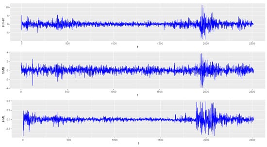
Figure 1. Time series plots of the three factors (Rm − Rf, SMB and HML).

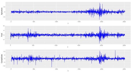
Figure 2. Time series plots of $y_{1t}$, $y_{2t}$ and $y_{3t}$.

In this example, we denote our portfolio allocation by FG, and compare it with the allocation proposed by [29] (denoted by Fan2008) in the terms of annualized Sharpe ratios. The calculation of annualized Sharpe ratio follows the trading strategy similar to [23]. Every year’s trading days are approximately $T=252$. All possible portfolio allocations are assumed attainable, short selling is admitted, and there is no transaction cost.

In the trading strategy, we form a portfolio allocation $\widehat{w}$ at the end of each trading day, and hold it until the end of the next trading day. Between day $t-1$ and t, we calculate the realized return as follows

$$\begin{array}{c}\hfill R_t\left(\widehat{w}\right)={\widehat{w}}^{\tau }{y}_t,\end{array}$$

with $\widehat{w}$ calculated based on $(x_{t-i},y_{t-i})$, for $i=1,\cdots ,n$, and $t=1,\cdots ,T$. Hence, the annualized Sharpe ratio is evaluated by

$$\begin{array}{c}\hfill \mathrm{SR}\left(\widehat{w}\right)=\frac{\overline{R}\left(\widehat{w}\right)}{\mathrm{sd}\left(\widehat{w}\right)}\sqrt{T},\end{array}$$

where

$$\begin{array}{c}\hfill \overline{R}\left(\widehat{w}\right)=\frac{1}{T}\sum _{t=1}^T[R_t\left(\widehat{w}\right)-R_{ft}],\mathrm{sd}\left(R\right)=\left\{\frac{1}{T}\sum _{t=1}^T{[R_t\left(\widehat{w}\right)-R_{ft}-\overline{R}\left(\widehat{w}\right)]}^2\right\},\end{array}$$

with $R_{ft}$ as the risk-free rate of day t. We calculate the annualized Sharpe ratios at the end of the final trading day of each year, and repeat this by using sample size $n=100$ and $n=500$.

Figure 3 shows the plots of the proposed annualized Sharpe ratios based on $n=$ 100 and 500 respectively. It is seen that the performance of the proposed annualized Sharpe ratio becomes better as sample size n increases.

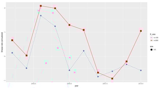
Figure 3. Annualized Sharpe ratios.

Furthermore, the performances of the two allocations in terms of Sharpe ratio are depicted in Figure 4. It is found that FG outperforms Fan2008 in the majority of the observations. This results can be attributed to the fact that there exists GARCH effect for the considered data. Consequently, the dynamic conditional covariance (FG) is expected to show certain superiority compared to the unconditional covariance (Fan2008).

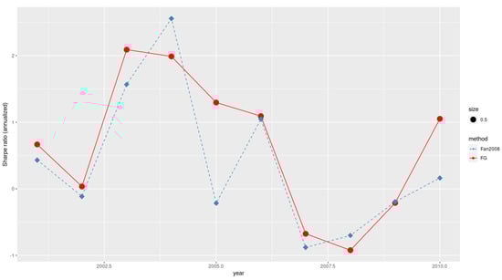
Figure 4. Annualized Sharpe ratios for $n=500$.

6. Conclusions

In this article, we proposed a factor-GARCH model for ultra-high dimensional conditional covariance. One advantage of the proposed model is that, when $p\ge T$ and both diverge, it can capture the dynamics of the conditional covariance matrix well and also guarantees that the estimated matrix is invertible. This plays an important role in practical applications. First, we use the popular factor model constructed by [34] to reduce the dimensions. Then, CCC-GARCH is imposed to fit the common factor vector.

Last, we use the univariate GARCH model to estimate the idiosyncratic errors of $y_t$. The loading factor matrix is estimated by the least square method, and QMLE is proposed to estimate the parameters in GARCH models. Then, we give the estimate of ${\Sigma }_y\left(t\right)$ by using the plug-in method. Asymptotic properties are derived for the estimation, and simulation studies are given to demonstrate its performance. A given financial application shows that the proposed model is of certain superiority compared to the existent models.

On the basis of this paper, several questions are worthy of further study. In the article, we investigated the case where the common factors are observable and K is known, and we assumed that idiosyncratic errors have univariate GARCH structure. However, in some occasions, the common factors may not be observable, the number of factors could be unknown, and the idiosyncratic errors might follow a more complicated structure. Hence, it makes sense to extend the proposed model to more general cases, and these are left for future studies.

References

- Bollerslev, T.; Engle, R.F.; Wooldridge, J.M. A Capital Asset Pricing Model With Time-varying Covariances. J. Politic. Econ. 1988, 96, 116–131. [Google Scholar] [CrossRef]
- Engle, R.; Kroner, K.F. Multivariate Simultaneous Generalized ARCH. Econom. Theor. 1995, 11, 122–150. [Google Scholar] [CrossRef]
- Bollerslev, T. Modelling the Coherence in Short-Run Nominal Exchange Rates: A Multivariate Generalized ARCH Model. Rev. Econ. Statist. 1990, 72, 498–505. [Google Scholar] [CrossRef]
- Engle, R. Dynamic Conditional Correlation: A Simple Class of Multivariate Generalized Autoregressive Conditional Heteroskedasticity Models. J. Bus. Econ. Statist. 2002, 20, 339–350. [Google Scholar] [CrossRef]
- Kroner, F.K.; Ng, V.K. Modelling asymmetric comovements of asset returns. Rev. Financ. Stud. 1998, 11, 817–844. [Google Scholar] [CrossRef]
- Hansson, B.; Hordahl, P. Testing the conditional CAPM using multivariate GARCH-M. Appl. Financ. Econm. 1998, 8, 377–388. [Google Scholar] [CrossRef]
- Bauwens, I.; Laurent, S.; Rombouts, J.V.K. Multivariate GARCH model: A survey. J. Appl. Econ. 2006, 21, 79–109. [Google Scholar] [CrossRef] [Green Version]
- Hafner, C.; Herwartz, H. Time-varying market price of risk in the CAPM. Approaches, empirical evidence and implications. Finance 1998, 9, 93–112. [Google Scholar]
- Francq, C.; Zakoïan, J.-M. Estimating multivariate GARCH models equation by equation. J. R. Stat. Soc.-Ser. B 2016, 78, 613–635. [Google Scholar] [CrossRef]
- Gao, Z.; Tsay, R. A structural-factor approach to modeling high-dimensional time series and space-time data. J. Time Ser. Anal. 2019, 40, 343–362. [Google Scholar] [CrossRef] [Green Version]
- Gao, Z.; Tsay, R. Modeling high-dimensional time series: A factor model with dynamically dependent factors and diverging eigenvalues. J. Am. Statist. Assoc. 2020, 1–44. [Google Scholar] [CrossRef]
- Lam, C.; Yao, Q.; Bathia, N. Estimation for latent factor models for high-dimensional time series. Biometrika 2011, 98, 901–918. [Google Scholar] [CrossRef]
- Lam, C.; Yao, Q. Factor modeling for high-dimensional time series: Inference for the number of factors. Ann. Statist. 2012, 40, 694–726. [Google Scholar] [CrossRef] [Green Version]
- Pan, J.; Yao, Q. Modelling multiple time series via common factors. Biometrika 2008, 95, 356–379. [Google Scholar] [CrossRef] [Green Version]
- Engle, R.; Ng, V.; Rothschild, M. Asset pricing with a factor-ARCH covariance structure: Empirical estimates for treasury bill. J. Econmetr. 1990, 45, 213–238. [Google Scholar] [CrossRef] [Green Version]
- Bollerslev, T.; Engle, R. Common persistence in conditional variances. Econometrica 1993, 61, 167–186. [Google Scholar] [CrossRef]
- Lin, W. Alternative estimators for factor GARCH model—A Monte Carlo comparison. J. Appl. Econ. 1992, 7, 259–279. [Google Scholar] [CrossRef]
- Vrontos, I.; Dellaportas, P.; Politis, D. A full-factor multivariate GARCH model. Econmetr. J. 2003, 6, 311–333. [Google Scholar] [CrossRef]
- Alexander, C. Orthogonal GARCH. In Mastering Risk; Financial Times-Prentice-Hall: London, UK, 2001; Volume 2, pp. 21–38. [Google Scholar]
- Van der Weide, R. GO-GARCH: A multivariate generalized orthogonal GARCH model. J. Appl. Econ. 2002, 17, 549–564. [Google Scholar] [CrossRef]
- Hafner, C.; Preminger, A. Asymptotic theory for a factor GARCH model. Econom. Theory 2009, 25, 336–363. [Google Scholar] [CrossRef]
- Fan, J.; Wang, M.; Yao, Q. Modelling multivariate volatilites via conditionally uncorrelated components. J. R. Statist. Soc. B 2008, 70, 679–702. [Google Scholar] [CrossRef] [Green Version]
- Guo, S.; Box, J.L.; Zhang, W. A Dynamic Structure for High-Dimensional Covariance Matrices and Its Application in Portfolio Allocation. J. Am. Statist. Assoc. 2017, 112, 235–253. [Google Scholar] [CrossRef]
- Fan, J.; Mincheva, L.M. High-dimensional covariance matrix estimation in approximate factor models. Ann. Statist. 2011, 39, 3320–3356. [Google Scholar] [CrossRef] [PubMed]
- Francq, C.; Zakoïan, J.-M. GARCH Modes: Structure, Statistical Inference and Financial Applications; John Wiley & Sons: Hoboken, NJ, USA, 2019. [Google Scholar]
- Fan, J.; Liao, Y.; Mincheva, M. Large covariance estimation by thresholding principal orthogonal complements. J. R. Stat. Soc.-Ser. B 2013, 75, 603–680. [Google Scholar] [CrossRef] [Green Version]
- Lindner, A.M. Stationarity, mixing, distributional properties and moments of GARCH(p, q) processes. In Handbook of Financial Time Series; Springer: Berlin/Heidelberg, Germany, 2009; pp. 43–69. [Google Scholar]
- Li, X.; Li, Y.; Pan, J.; Zhang, X. A Factor-GARCH Model for High Dimensional Volatilities. Guangzhou University, Guangzhou, China. Unpublished manuscript.
- Fan, J.; Fan, Y.; Lv, J. High dimensional covariance matrix estimation using a factor model. J. Econmetr. 2008, 147, 186–197. [Google Scholar] [CrossRef] [Green Version]
- James, W.; Stein, C. Estimation with quadratic loss. In Proceedings of the Fourth Berkeley Symposium on Mathematical Statistics and Probability, Volume 1: Contributions to the Theory of Statistics; University of California Press: Berkeley, CA, USA, 1961; pp. 361–379. [Google Scholar]
- Tsay, R.S. Multivariate Time Series Analysis; John Wiley & Sons: Hoboken, NJ, USA, 2014. [Google Scholar]
- Markowitz, H.M. Portfolio selection. J. Financ. 1952, 7, 77–91. [Google Scholar]
- Markowitz, H.M. Portfolio Selection: Efficient Diversification of Investments; John Wiley & Sons: Hoboken, NJ, USA, 1959. [Google Scholar]
- Fama, E.; French, K. The cross-section of expected stock returns. J. Financ. 1992, 47, 427–465. [Google Scholar] [CrossRef]
Publisher’s Note: MDPI stays neutral with regard to jurisdictional claims in published maps and institutional affiliations. |
© 2022 by the authors. Licensee MDPI, Basel, Switzerland. This article is an open access article distributed under the terms and conditions of the Creative Commons Attribution (CC BY) license (https://creativecommons.org/licenses/by/4.0/).