
Effect of Pulsatility on the Transport of Thrombin in an Idealized Cerebral Aneurysm Geometry

 , , and
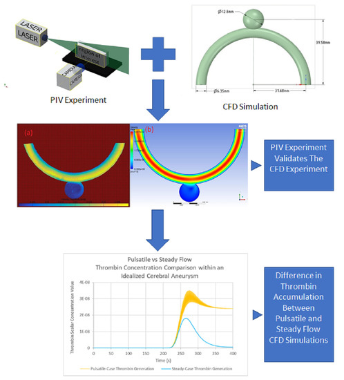
Abstract
1. Introduction
2. Materials and Methods
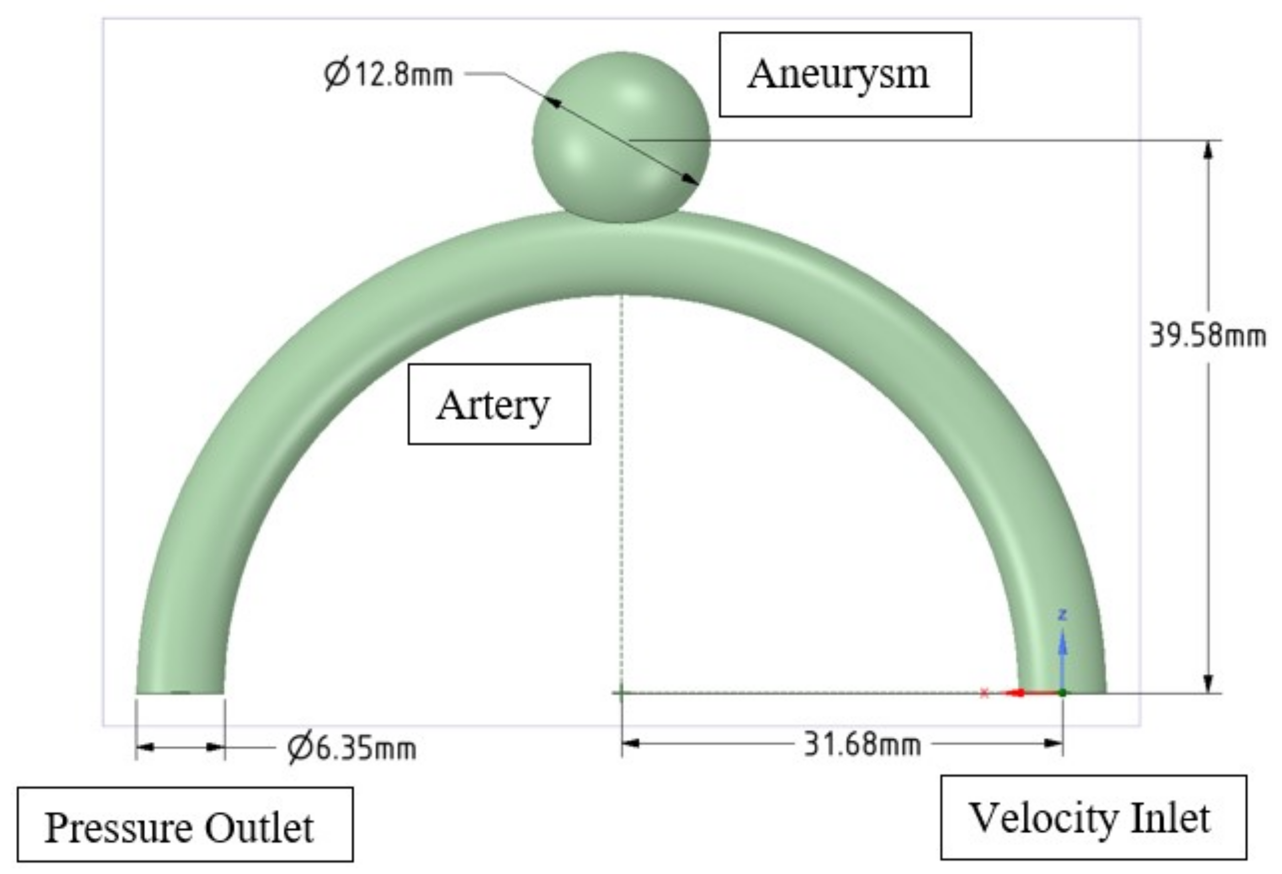
2.1. Idealised Geometry
2.2. Experimental Study
2.2.1. Symmetrical Idealised Phantom
2.2.2. Working Fluid
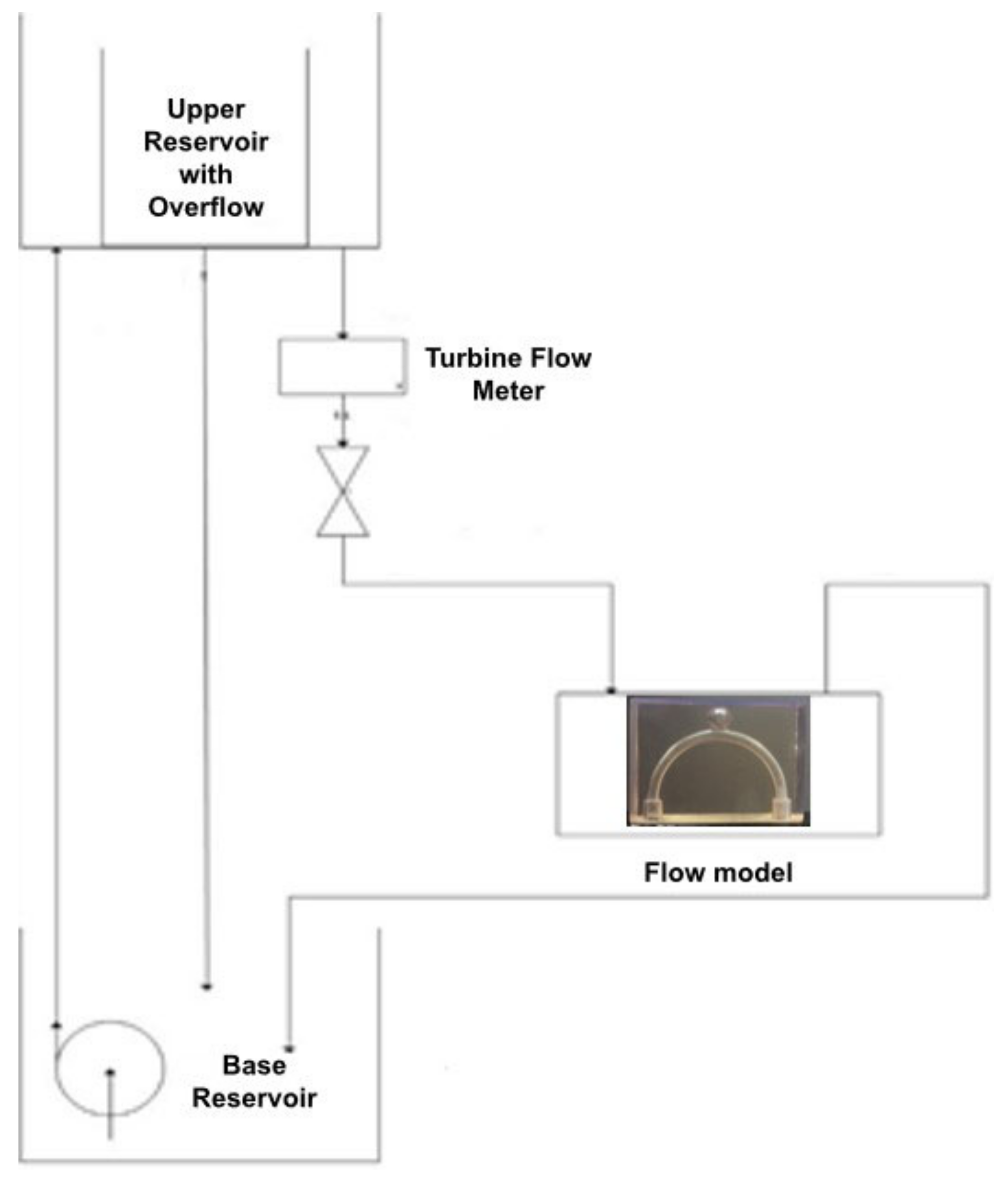
2.2.3. Flow Circuit
2.2.4. PIV Setup
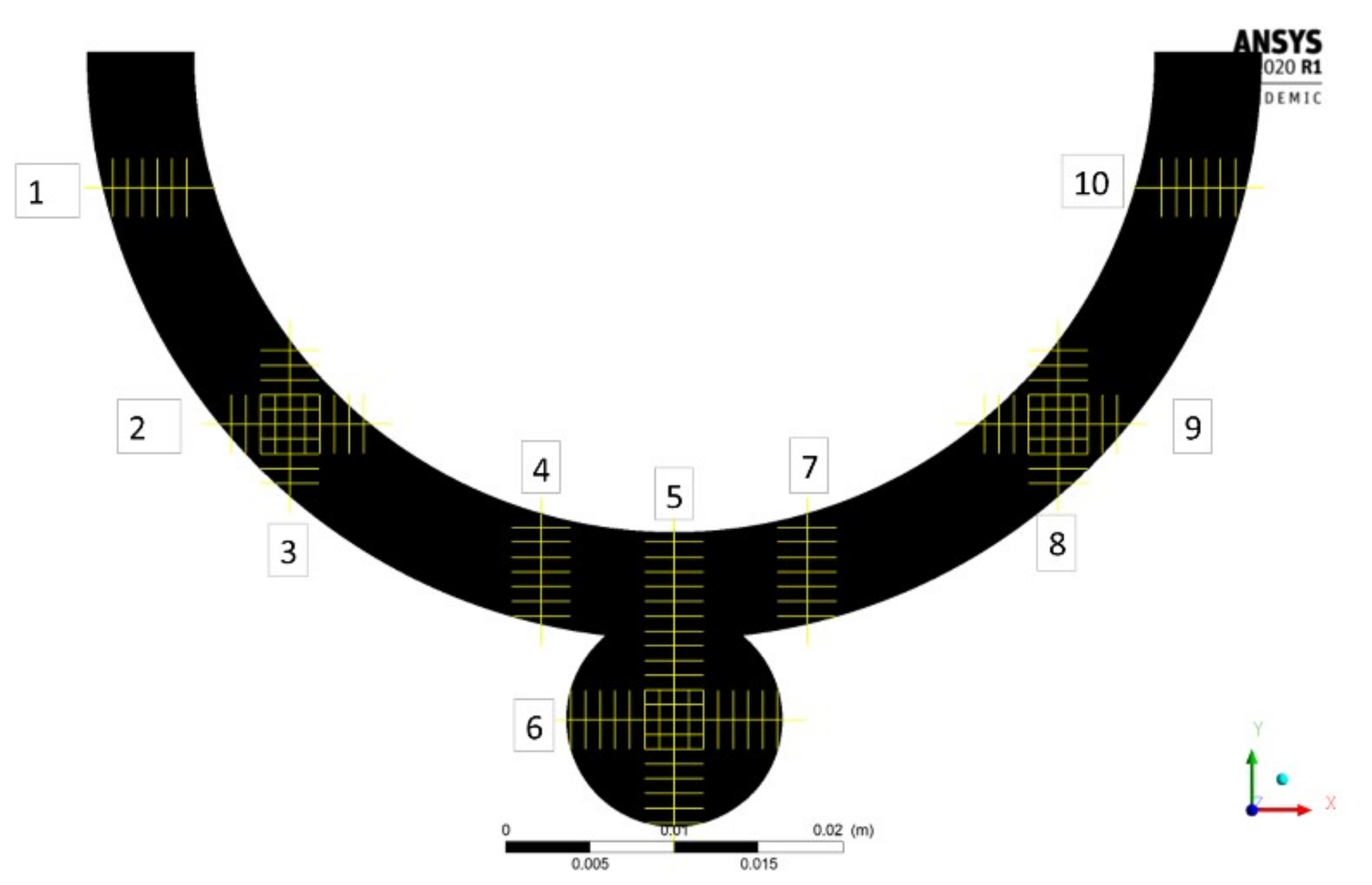
2.2.5. Processing of PIV Measurements
2.3. Numerical Simulations
2.3.1. Navier–Stokes Equations
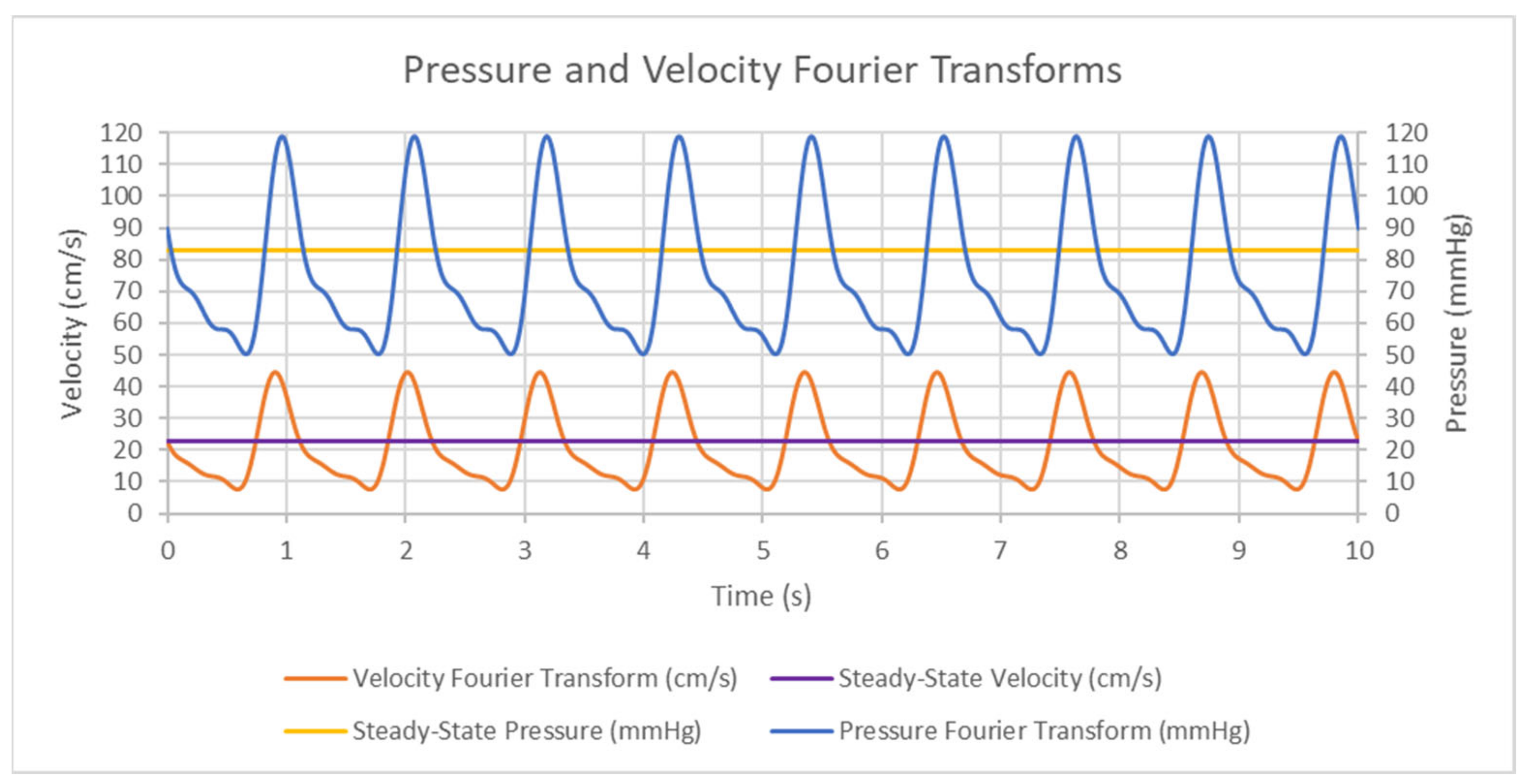
2.3.2. Boundary Conditions
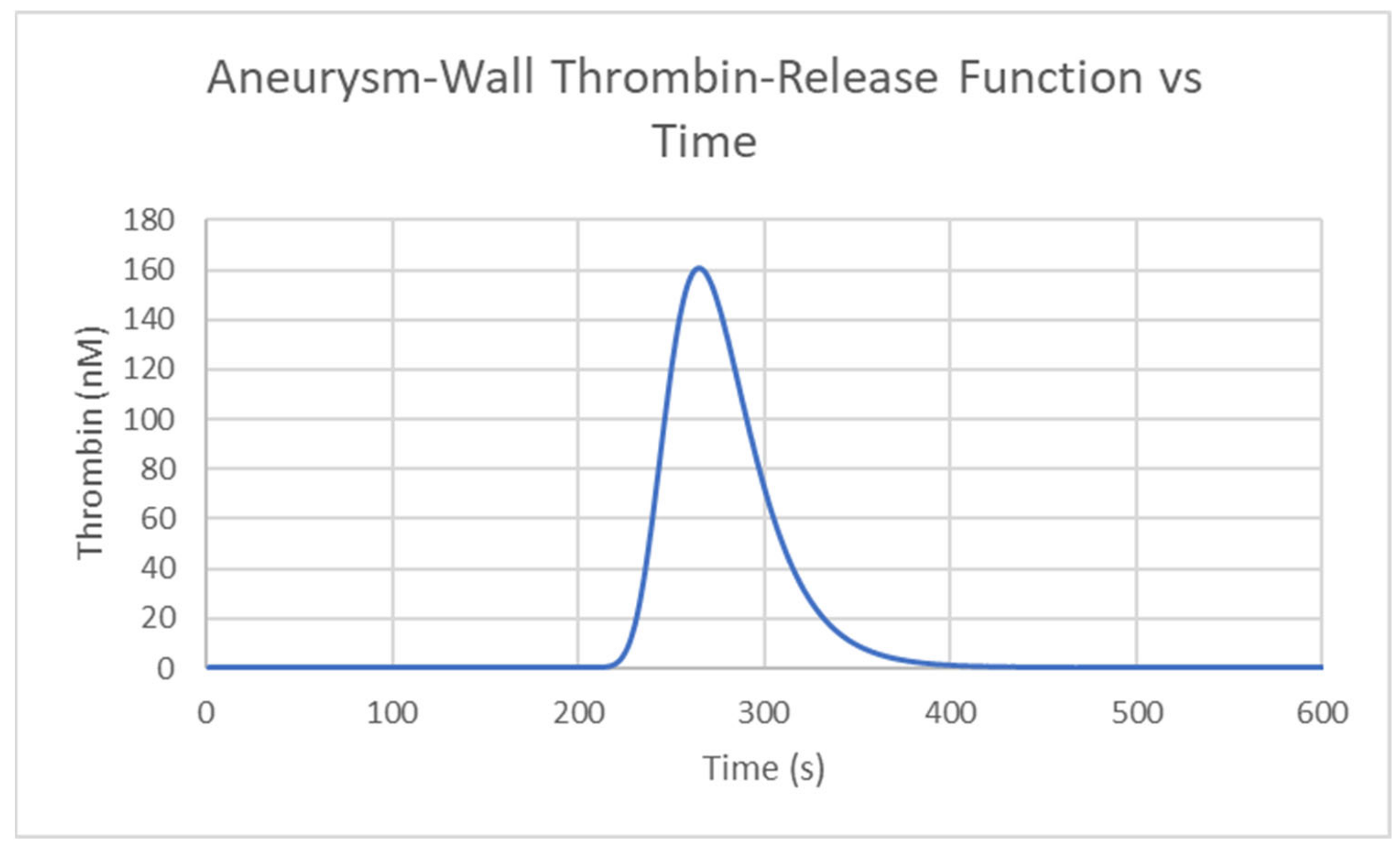
2.3.3. Transport Equation for the Description of Thrombin
2.3.4. Solver Settings
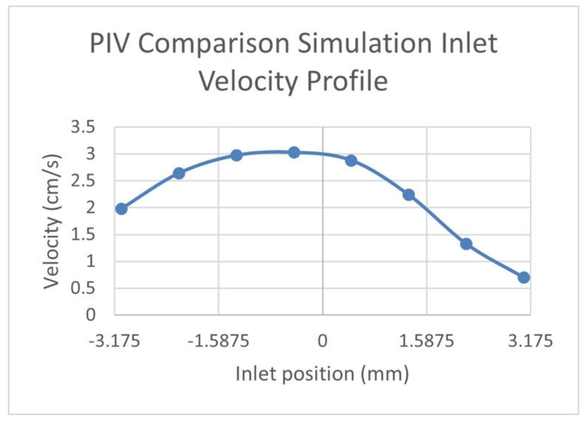
2.3.5. PIV Comparison Simulation
3. Results
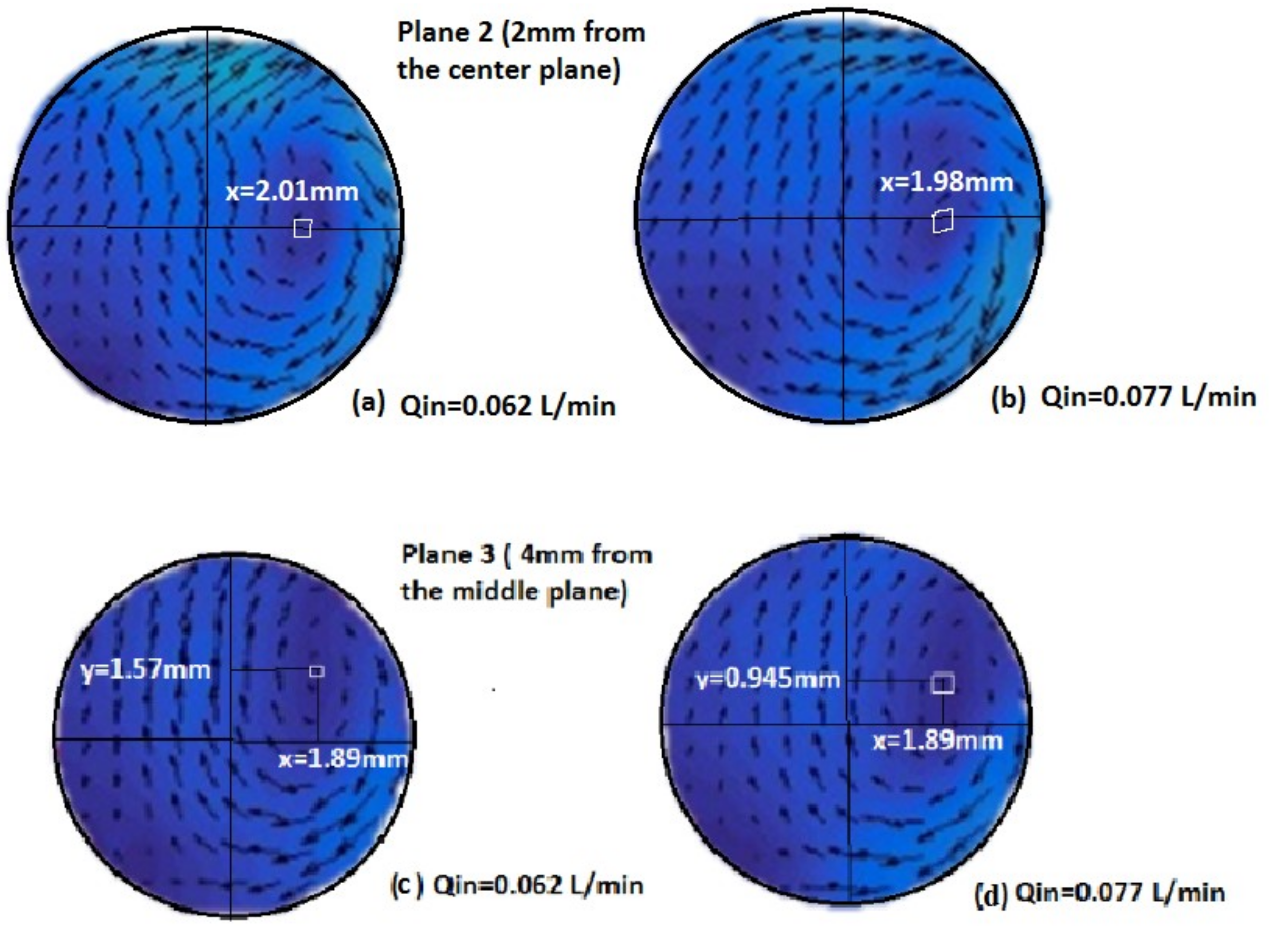
3.1. Experimental Results
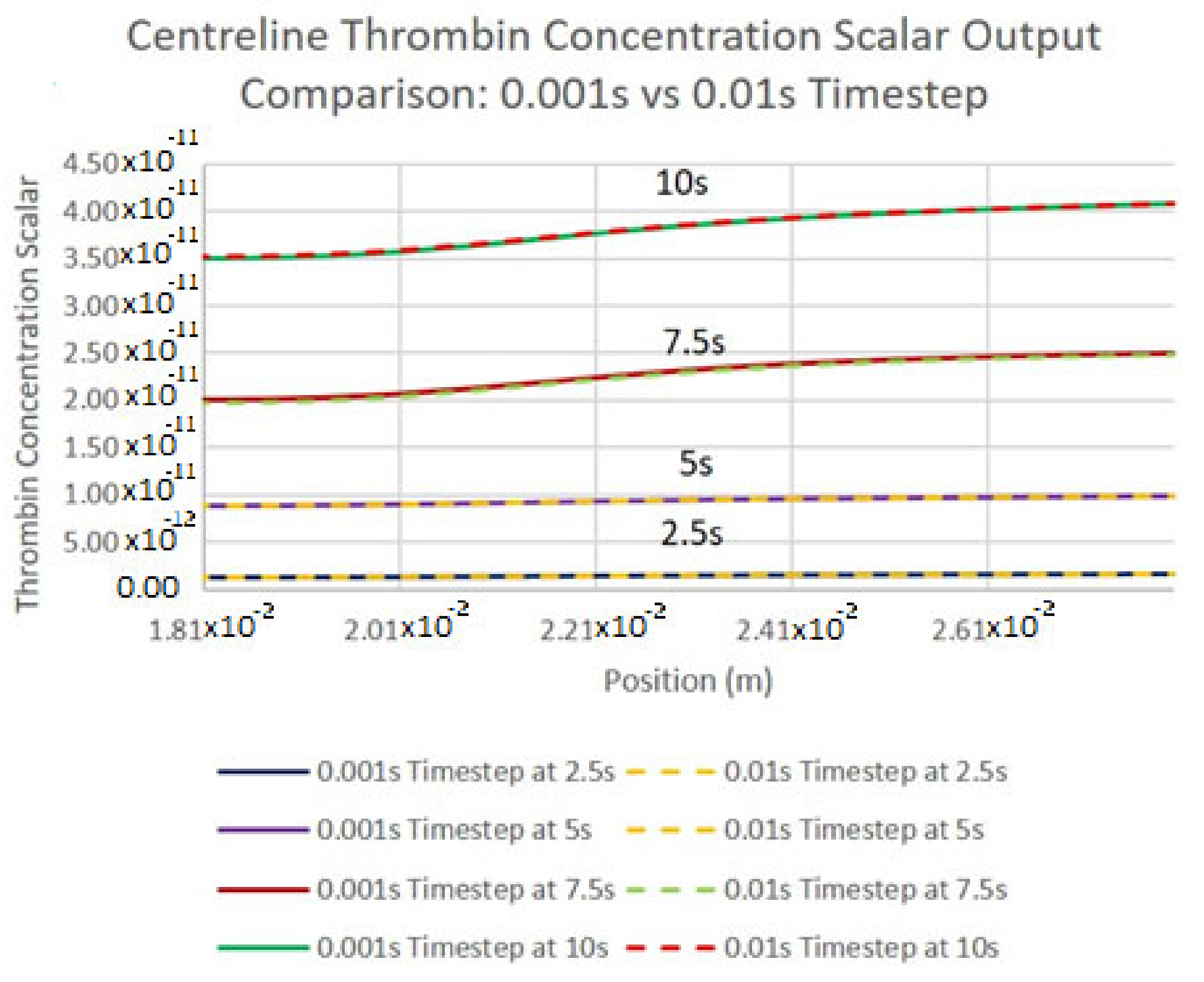
3.2. Grid Independence for Numerical Results
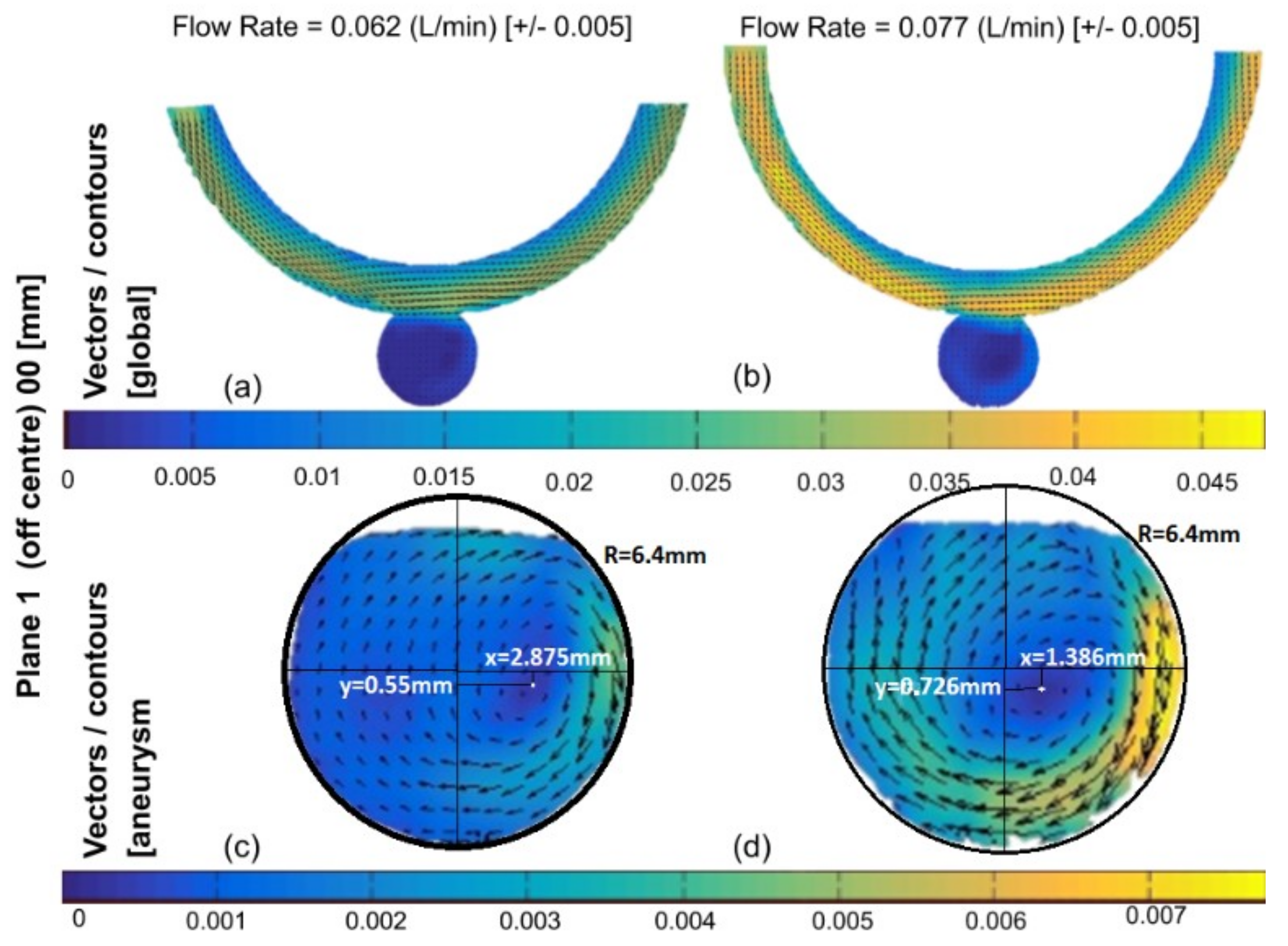
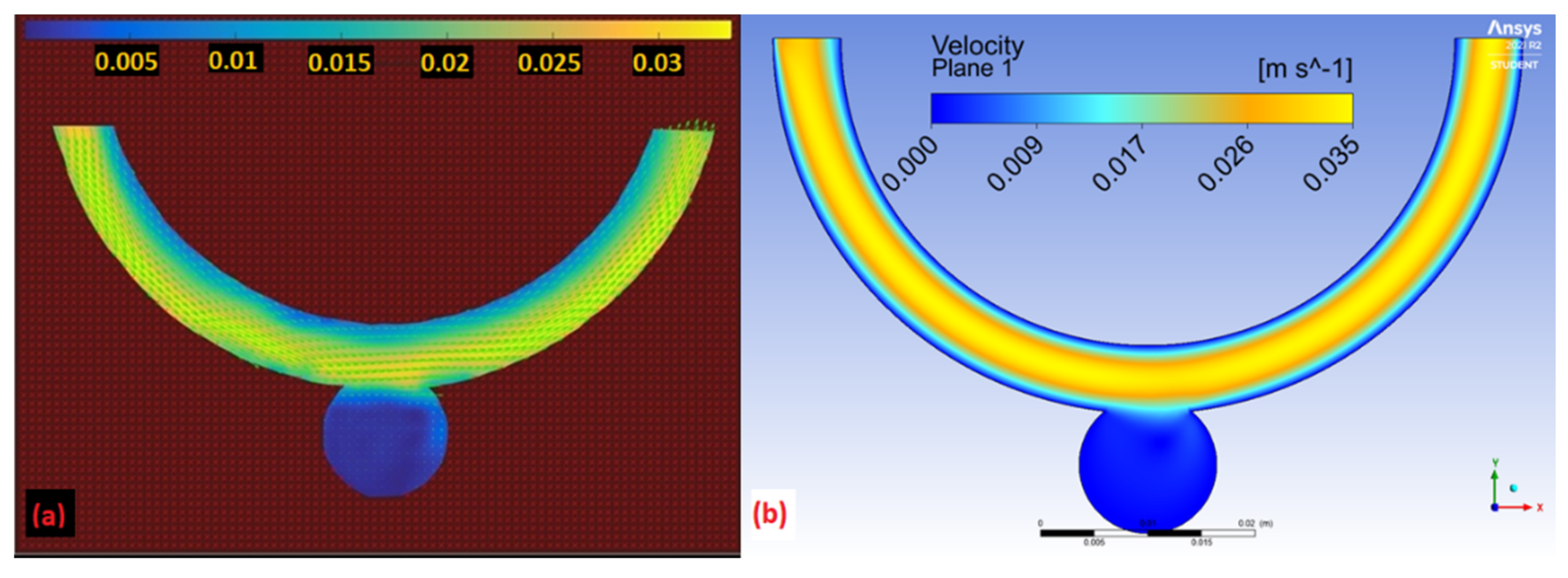
3.3. Comparison of Experimental and Numerical Results
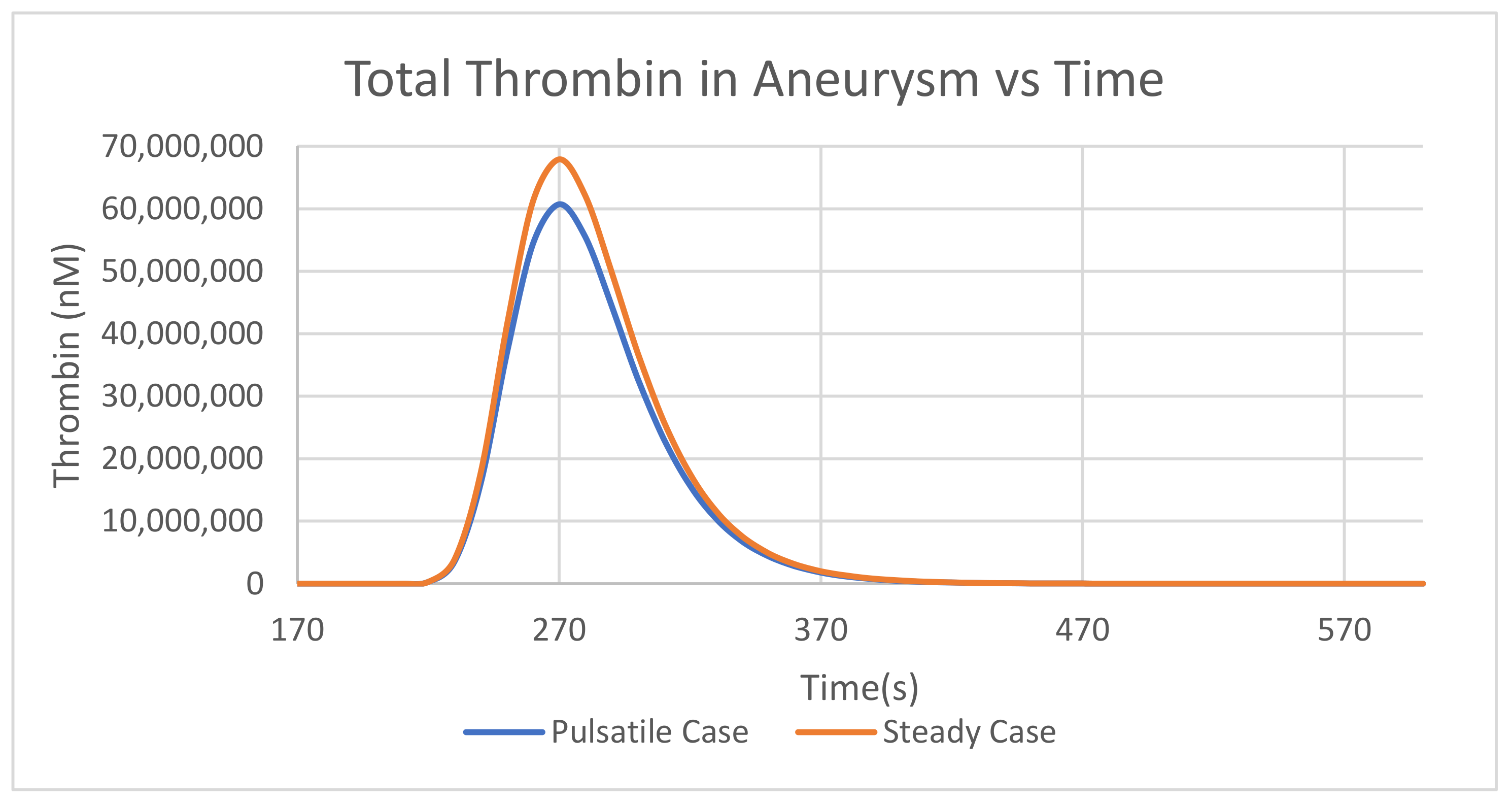
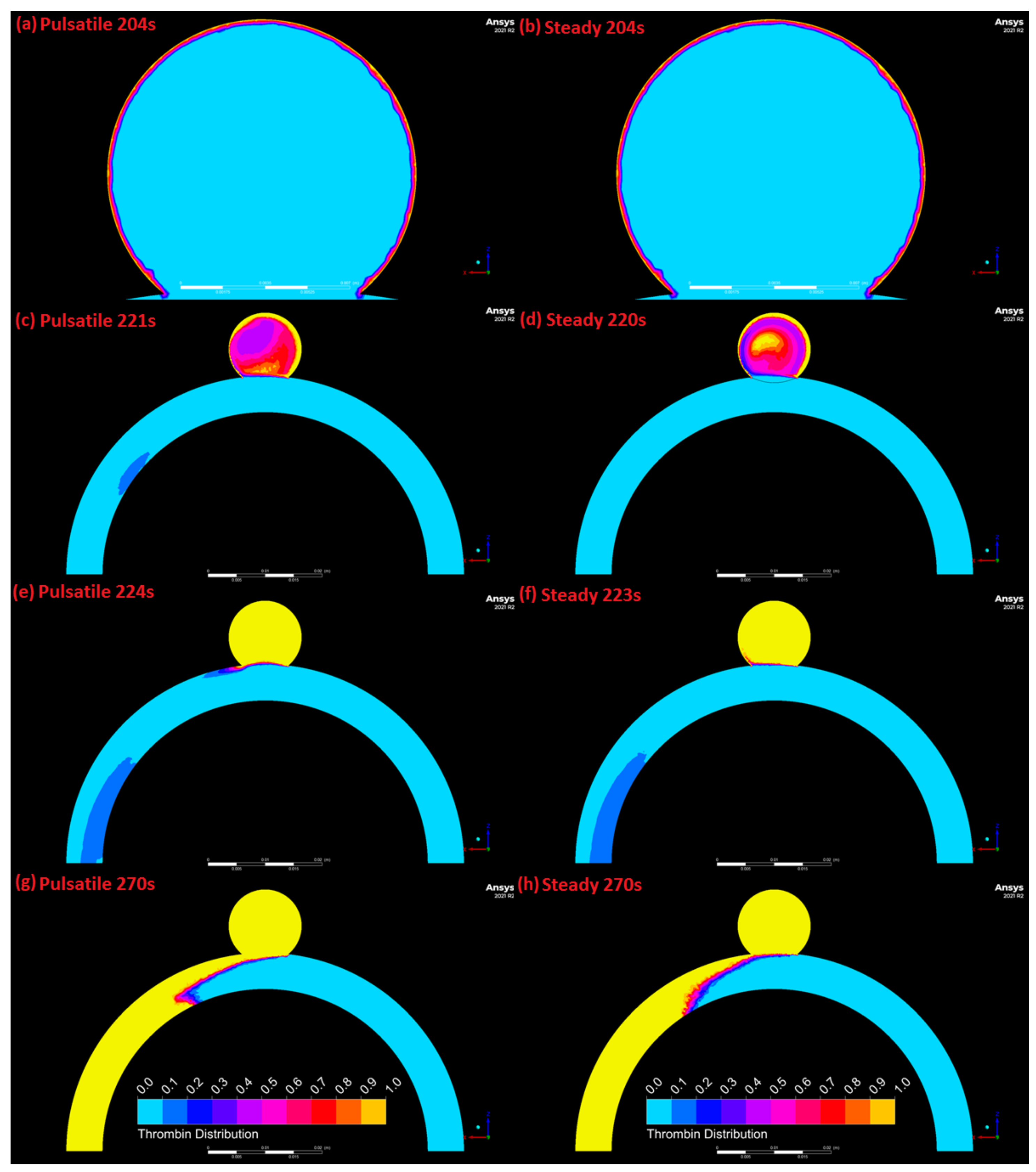
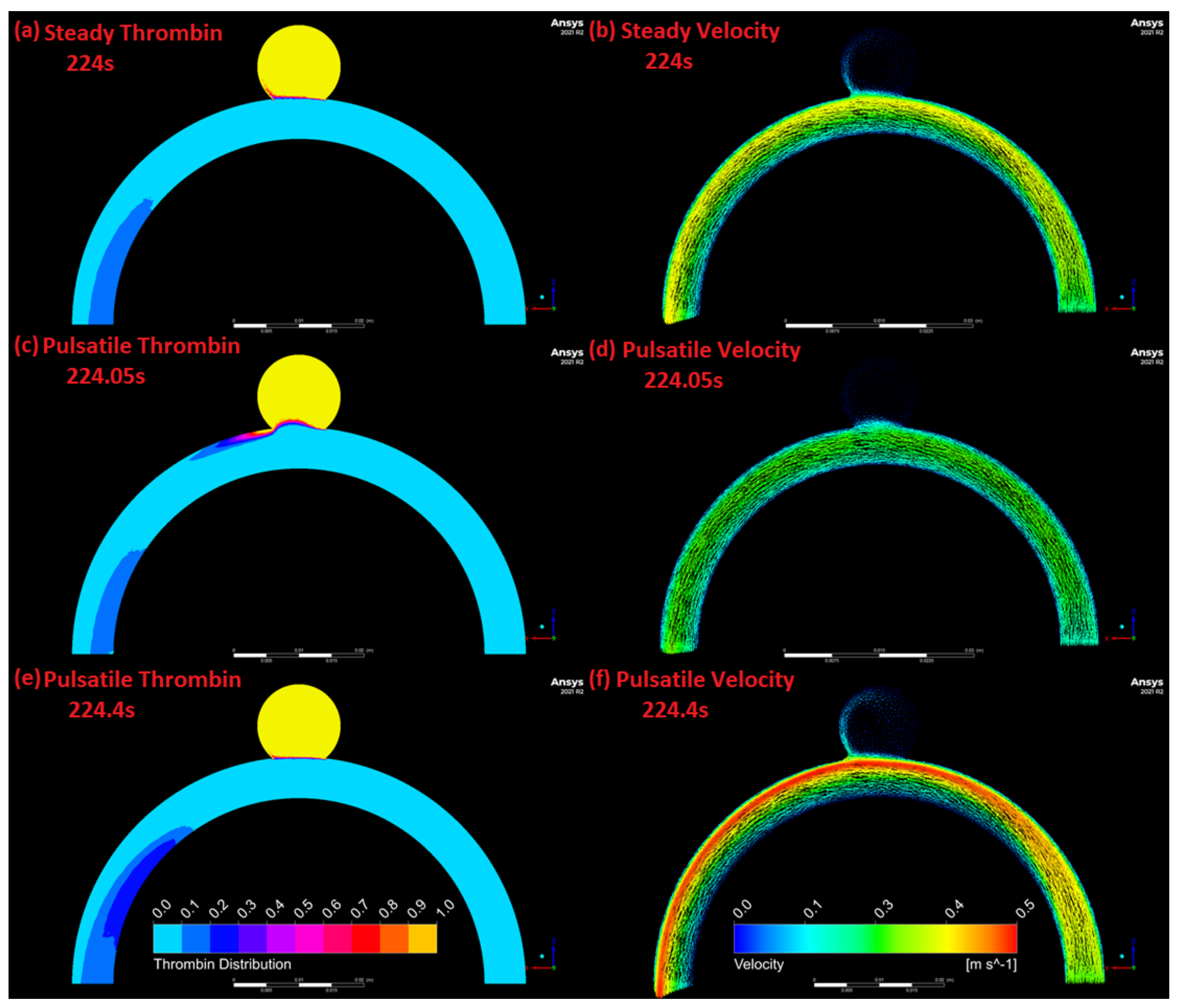
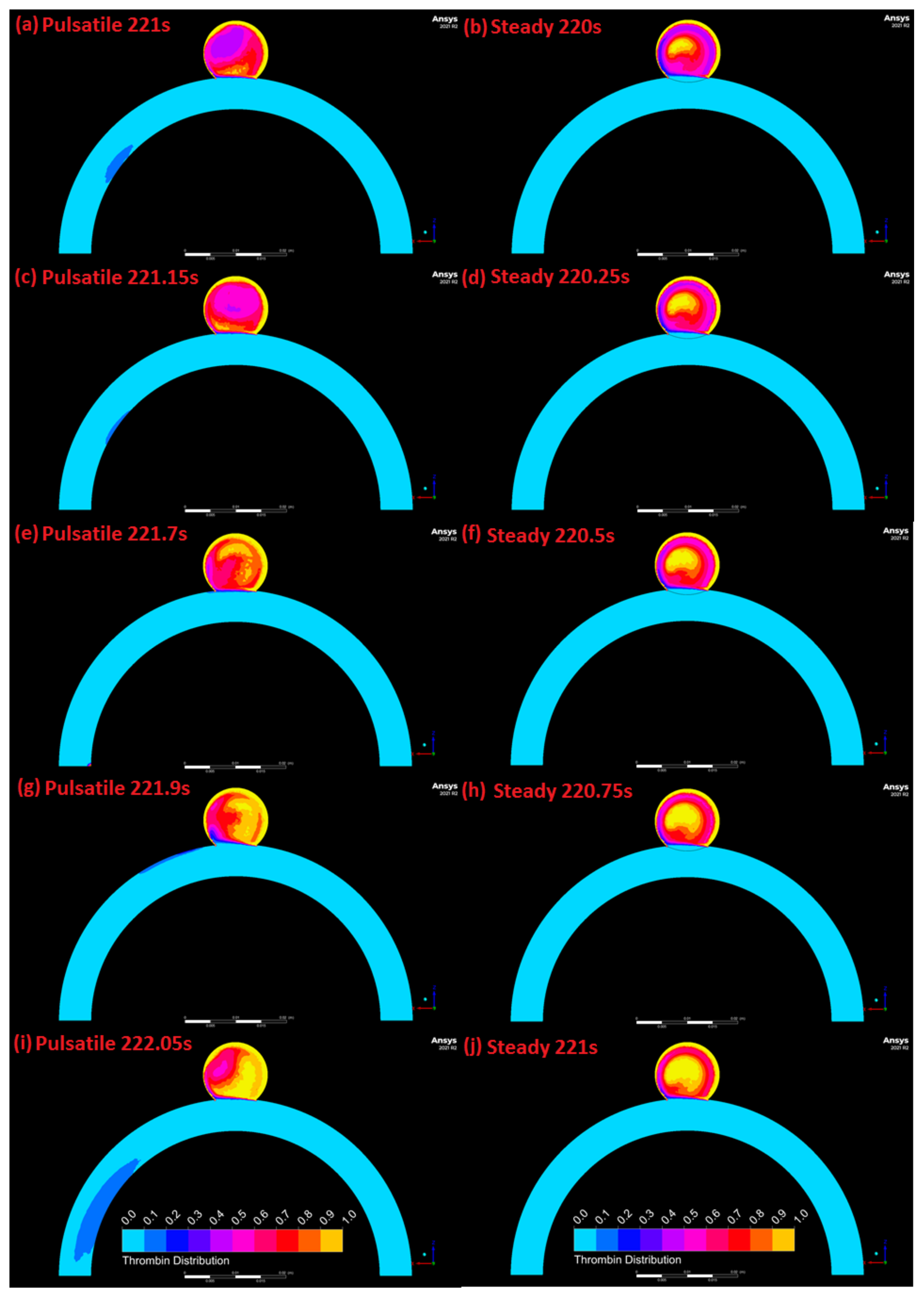
3.4. Comparison of Pulsatile and Steady State Numerical Results
4. Discussion
5. Conclusions
Author Contributions
Funding
Data Availability Statement
Conflicts of Interest
References
- Lawton, M.T.; Quiones-Hinojosa, A.; Chang, E.F.; Yu, T. Thrombotic Intracranial Aneurysms: Classification Scheme and Management Strategies in 68 Patients. Neurosurgery 2005, 56, 441–454. [Google Scholar] [CrossRef]
- Eller, T.W. MRI demonstration of clot in a small unruptured aneurysm causing stroke. Case report. J. Neurosurg. 1986, 65, 411–412. [Google Scholar] [CrossRef] [PubMed]
- Ishikawa, T.; Nakayama, N.; Yoshimoto, T.; Aoki, T.; Terasaka, S.; Nomura, M.; Takahashi, A.; Kuroda, S.; Iwasaki, Y. How does spontaneous hemostasis occur in ruptured cerebral aneurysms? Preliminary investigation on 247 clipping surgeries. Surg. Neurol. 2006, 66, 269–275. [Google Scholar] [CrossRef]
- Calviere, L.; Viguier, A.; da Silva, N.A.; Cognard, C.; Larrue, V. Unruptured intracranial aneurysm as a cause of cerebral ischemia. Clin. Neurol. Neurosurg. 2011, 113, 28–33. [Google Scholar] [CrossRef] [PubMed]
- Ngoepe, M.N.; Frangi, A.F.; Byrne, J.V.; Ventikos, Y. Thrombosis in cerebral aneurysms and the computational modeling thereof: A review. Front. Physiol. 2018, 9, 1–22. [Google Scholar] [CrossRef]
- Rigano, J.; Ng, C.; Nandurkard, H.; Ho, P. Thrombin generation estimates the anticoagulation effect of direct oral anticoagulants with significant interindividual variability observed. Blood Coagul. Fibrinolysis 2018, 29, 148–154. [Google Scholar] [CrossRef]
- Scanarini, M.; Mingrino, S.; Giordano, R.; Baroni, A. Histological and ultrastructural study of intracranial saccular aneurysmal wall. Acta Neurochir. 1978, 43, 171–182. [Google Scholar] [CrossRef] [PubMed]
- Humphrey, J.D.; Canham, P.B. Structure, Mechanical Properties, and Mechanics of Intracranial Saccular Aneurysms. J. Elast. 2000, 61, 49–81. [Google Scholar] [CrossRef]
- Orfeo, T.; Butenas, S.; Brummel-Ziedins, K.E.; Mann, K.G. The tissue factor requirement in blood coagulation. J. Biol. Chem. 2005, 280, 42887–42896. [Google Scholar] [CrossRef]
- Sutherland, G.R.; King, M.E.; Peerless, S.J.; Vezina, W.C.; Brown, G.W.; Chamberlain, M.J. Platelet interaction within giant intracranial aneurysms. J. Neurosurg. 1982, 56, 53–61. [Google Scholar] [CrossRef] [PubMed]
- Giesen, P.L.; Rauch, U.; Bohrmann, B.; Kling, D.; Roqué, M.; Fallon, J.T.; Badimon, J.J.; Himber, J.; Riederer, M.A.; Nemerson, Y. Blood-borne tissue factor: Another view of thrombosis. Proc. Natl. Acad. Sci. USA 1999, 96, 2311–2315. [Google Scholar] [CrossRef]
- Hathcock, J.J.; Nemerson, Y. Platelet deposition inhibits tissue factor activity: In vitro clots are impermeable to factor Xa. Blood 2004, 104, 123–127. [Google Scholar] [CrossRef]
- Morel, O.; Jesel, L.; Freyssinet, J.-M.; Toti, F. Cellular mechanisms underlying the formation of circulating microparticles. Arterioscler. Thromb. Vasc. Biol. 2011, 31, 15–26. [Google Scholar] [CrossRef] [PubMed]
- Peach, T.W.; Ngoepe, M.; Spranger, K.; Ventikos, Y. Personalizing flow-diverter intervention for cerebral aneurysms: From computational hemodynamics to biochemical modeling. Int. J. Numer. Methods Biomed. Eng. 2014, 1–21. [Google Scholar] [CrossRef]
- Rayz, V.L.; Boussel, L.; Lawton, M.T.; Acevedo-Bolton, G.; Ge, L.; Young, W.L.; Higashida, R.T.; Saloner, D. Numerical modeling of the flow in intracranial aneurysms: Prediction of regions prone to thrombus formation. Ann. Biomed. Eng. 2008, 36, 1793–1804. [Google Scholar] [CrossRef]
- Di Achille, P.; Tellides, G.; Figueroa, C.A.; Humphrey, J.D. A haemodynamic predictor of intraluminal thrombus formation in abdominal aortic aneurysms. Proc. R. Soc. London A Math. Phys. Eng. Sci. 2014, 470, 20140163. [Google Scholar] [CrossRef]
- Ngoepe, M.; Ventikos, Y. Computational modelling of clot development in patient- specific cerebral aneurysm cases. J. Thromb. Haemost. 2016, 14, 262–272. [Google Scholar] [CrossRef] [PubMed]
- Ou, C.; Huang, W.; Yuen, M.M.F. A computational model based on fibrin accumulation for the prediction of stasis thrombosis following flow-diverting treatment in cerebral aneurysms. Med. Biol. Eng. Comput. 2016, 55, 1–11. [Google Scholar] [CrossRef]
- Sarrami-Foroushani, A.; Lassila, T.; Hejazi, S.M.; Nagaraja, S.; Bacon, A.; Frangi, A.F. A computational model for prediction of clot platelet content in flow-diverted intracranial aneurysms. J. Biomech. 2019, 91, 7–13. [Google Scholar] [CrossRef] [PubMed]
- Moriguchi, T.; Sumpio, B.E. PECAM-1 phosphorylation and tissue factor expression in HUVECs exposed to uniform and disturbed pulsatile flow and chemical stimuli. J. Vasc. Surg. 2015, 61, 481–488. [Google Scholar] [CrossRef][Green Version]
- Steadman, E.; Laljee, S.; Fandaros, M.; Rubenstein, D.; Yin, W. Thrombin Generation Kinetics Under Constant and Pulsatile Shear Stress. FASEB J. 2019, 33, 522–527. [Google Scholar]
- Corbett, S.C.; Ajdari, A.; Coskun, A.U.; Nayeb-Hashemi, H. Effect of pulsatile blood flow on thrombosis potential with a step wall transition. ASAIO J. 2010, 56, 290–295. [Google Scholar] [CrossRef]
- Cavazzuti, M.; Atherton, M.A.; Collins, M.W.; Barozzi, G.S. Non-Newtonian and flow pulsatility effects in simulation models of a stented intracranial aneurysm. Proc. Inst. Mech. Eng. Part. H J. Eng. Med. 2011, 225, 597–609. [Google Scholar] [CrossRef] [PubMed]
- Mulder, G.; Bogaerds, A.C.B.; Rongen, P.; Vosse, F.N. On automated analysis of flow patterns in cerebral aneurysms based on vortex identification. J. Eng. Math. 2009, 64, 391–401. [Google Scholar] [CrossRef]
- Ho, W.H.; Tshimanga, I.J.; Ngoepe, M.N.; Jermy, M.C.; Geoghegan, P.H. Evaluation of a Desktop 3D Printed Rigid Refractive-Indexed-Matched Flow Phantom for PIV Measurements on Cerebral Aneurysms. Cardiovasc. Eng. Technol. 2019, 11, 24–28. [Google Scholar] [CrossRef]
- Jermy, M.C. Making it clear: Flexible, transparent laboratory flow models for soft and hard problems. In Proceedings of the 8th World Conference on Experimental Heat Transfer, Fluid Mechanics, and Thermodynamics, Lisbon, Portugal, 16–20 June 2013; pp. 1–8. [Google Scholar]
- Borrero-Echeverry, D.; Morrison, B.C.A. Aqueous ammonium thiocyanate solutions as refractive index-matching fluids with low density and viscosity. Exp. Fluids 2016, 57, 1–5. [Google Scholar] [CrossRef]
- Cebral, J.R.; Putman, C.M.; Alley, M.T.; Hope, T.; Bammer, R.; Calamante, F. Hemodynamics in Normal Cerebral Arteries: Qualitative Comparison of 4D Phase-Contrast Magnetic Resonance and Image-Based Computational Fluid Dynamics. J. Eng. Math. 2009, 64, 367–378. [Google Scholar] [CrossRef]
- Geoghegan, P.H.; Buchmann, N.A.; Spence, C.J.T.; Moore, S.; Jermy, M. Fabrication of rigid and flexible refractive-index-matched flow phantoms for flow visualisation and optical flow measurements. Exp. Fluids 2012, 52, 1331–1347. [Google Scholar] [CrossRef]
- Raffel, M.; Willert, C.E.; Wereley, S.T.; Kompenhans, J. Particle Image Velocimetry: A Practical Guide; Springer: Berlin/Heidelberg, Germany, 2002. [Google Scholar]
- Mendez, M.A.; Raiola, M.; Masullo, A.; Discetti, S.; Ianiro, A.; Theunissen, R.; Buchlin, J.M. POD-based background removal for particle image velocimetry. Exp. Therm. Fluid Sci. 2017, 80, 181–192. [Google Scholar] [CrossRef]
- Thielicke, W.; Stamhuis, E.J. PIVlab—Time-Resolved Digital Particle Image Velocimetry Tool for MATLAB 2010; MathWorks: Natick, MA, USA, 2010; pp. 1–4. [Google Scholar]
- Kundu, P.K.; Cohen, I.M. Fluid Mechanics, 4th ed.; Elsevier Inc.: Amsterdam, The Netherlands, 2008; ISBN 978-0-12-373735-9. [Google Scholar]
- Ferns, S.P.; Schneiders, J.J.; Siebes, M.; Van Den Berg, R.; Van Bavel, E.T.; Majoie, C.B. Intracranial blood-flow velocity and pressure measurements using an intra-arterial dual-sensor guidewire. Am. J. Neuroradiol. 2010, 31, 324–326. [Google Scholar] [CrossRef]
- Kremers, R.M.W.; de Laat, B.; Wagenvoord, R.J.; Hemker, H.C. Computational modelling of clot development in patient-specific cerebral aneurysm cases: Rebuttal. J. Thromb. Haemost. 2017, 15, 399. [Google Scholar] [CrossRef] [PubMed][Green Version]
- Ngoepe, M.; Passos, A.; Balabani, S.; King, J.; Lynn, A.; Moodley, J.; Swanson, L.; Bezuidenhout, D.; Davies, N.H.; Franz, T. A Preliminary Computational Investigation Into the Flow of PEG in Rat Myocardial Tissue for Regenerative Therapy. Front. Cardiovasc. Med. 2019, 6, 104. [Google Scholar] [CrossRef] [PubMed]
- Ouared, R.; Chopard, B.; Stahl, B.; Rüfenacht, D.A.; Yilmaz, H.; Courbebaisse, G. Thrombosis modeling in intracranial aneurysms: A lattice Boltzmann numerical algorithm. Comput. Phys. Commun. 2008, 179, 128–131. [Google Scholar] [CrossRef]
- Lieber, B.B.; Giddens, D.P. Post-stenotic core flow behavior in pulsatile flow and its effects on wall shear stress. J. Biomech. 1990, 23, 597–605. [Google Scholar] [CrossRef]
- Gester, K.; Lu, I.; Bu, M. In Vitro Evaluation of Intra-Aneurysmal, Flow-Diverter-Induced. Am. J. Neuroradiol. 2016, 37, 490–496. [Google Scholar] [CrossRef]


| Error from Baseline Mesh | ||||||
|---|---|---|---|---|---|---|
| Inlet | Centre-Axis Line Probe | Outlet Line Probe | ||||
| Elements in Mesh | Velocity | Pressure | Velocity | Pressure | Velocity | Pressure |
| 401,283 (Baseline) | 0% | 0% | 0% | 0% | 0% | 0% |
| 203,369 | 0% | 0.03% | 2.61% | 0.02% | 3.87% | 0.02% |
| 100,071 | 0% | 0.03% | 4.89% | 0.01% | 4.32% | 0.03% |
| PIV Simulation Deviation from Experimental Results | |
|---|---|
| Location | Velocity Magnitude |
| 1 | 6.46% |
| 2 | 5.86% |
| 3 | 16.10% |
| 4 | 13.02% |
| 5 | 9.46% |
| 6 | 29.67% |
| 7 | 8.63% |
| 8 | 10.78% |
| 9 | 7.48% |
| 10 | 21.21% |
| Average deviation | 12.87% |
Publisher’s Note: MDPI stays neutral with regard to jurisdictional claims in published maps and institutional affiliations. |
© 2022 by the authors. Licensee MDPI, Basel, Switzerland. This article is an open access article distributed under the terms and conditions of the Creative Commons Attribution (CC BY) license (https://creativecommons.org/licenses/by/4.0/).
Share and Cite
Hume, S.; Tshimanga, J.-M.I.; Geoghegan, P.; Malan, A.G.; Ho, W.H.; Ngoepe, M.N. Effect of Pulsatility on the Transport of Thrombin in an Idealized Cerebral Aneurysm Geometry. Symmetry 2022, 14, 133. https://doi.org/10.3390/sym14010133
Hume S, Tshimanga J-MI, Geoghegan P, Malan AG, Ho WH, Ngoepe MN. Effect of Pulsatility on the Transport of Thrombin in an Idealized Cerebral Aneurysm Geometry. Symmetry. 2022; 14(1):133. https://doi.org/10.3390/sym14010133
Chicago/Turabian StyleHume, Struan, Jean-Marc Ilunga Tshimanga, Patrick Geoghegan, Arnaud G. Malan, Wei Hua Ho, and Malebogo N. Ngoepe. 2022. "Effect of Pulsatility on the Transport of Thrombin in an Idealized Cerebral Aneurysm Geometry" Symmetry 14, no. 1: 133. https://doi.org/10.3390/sym14010133
APA StyleHume, S., Tshimanga, J.-M. I., Geoghegan, P., Malan, A. G., Ho, W. H., & Ngoepe, M. N. (2022). Effect of Pulsatility on the Transport of Thrombin in an Idealized Cerebral Aneurysm Geometry. Symmetry, 14(1), 133. https://doi.org/10.3390/sym14010133