A Solution of the Junction Riemann Problem for 1D Hyperbolic Balance Laws in Networks including Supersonic Flow Conditions on Elastic Collapsible Tubes

Abstract

The numerical modeling of one-dimensional (1D) domains joined by symmetric or asymmetric bifurcations or arbitrary junctions is still a challenge in the context of hyperbolic balance laws with application to flow in pipes, open channels or blood vessels, among others. The formulation of the Junction Riemann Problem (JRP) under subsonic conditions in 1D flow is clearly defined and solved by current methods, but they fail when sonic or supersonic conditions appear. Formulations coupling the 1D model for the vessels or pipes with other container-like formulations for junctions have been presented, requiring extra information such as assumed bulk mechanical properties and geometrical properties or the extension to more dimensions. To the best of our knowledge, in this work, the JRP is solved for the first time allowing solutions for all types of transitions and for any number of vessels, without requiring the definition of any extra information. The resulting JRP solver is theoretically well-founded, robust and simple, and returns the evolving state for the conserved variables in all vessels, allowing the use of any numerical method in the resolution of the inner cells used for the space-discretization of the vessels. The methodology of the proposed solver is presented in detail. The JRP solver is directly applicable if energy losses at the junctions are defined. Straightforward extension to other 1D hyperbolic flows can be performed.

1. Introduction

Numerical modeling of one-dimensional (1D) flow in networks of spatial domains joined by junctions offers a satisfactory compromise between the quality of the numerical predictions and the computational cost. There are a variety of 1D flow applications in the literature such as industrial piping networks, traffic flow, water flows in open channels or blood flow in the human circulatory system [1]. Flow physics at the bifurcation is complex in symmetric or asymmetric bifurcations and also in arbitrary junctions. One-dimensional modeling has proven to be an accurate tool in complex applications, such as computational hemodynamics in deformable arterial models under pulsatile flow, leading to competitive results if compared with three-dimensional (3D) simulations [2,3]. Flow in elastic and collapsible tubes is of great interest, and especially in the context of hemodynamics, physiology and medicine, and has been analyzed in many studies [4,5,6,7,8,9,10,11] in the last few decades.

However, the numerical modelling of 1D flow in networks is still challenging. In the 1D framework the junction is a singular point, where the numerical scheme cannot be directly applied and therefore internal boundary conditions must be prescribed [12], leading to the Junction Riemann Problem (JRP). A shortcoming of existing methods is their inability to deal with discontinuities or high subcritical, transcritical and supercritical flow through junctions, as in 1D channel networks, or to deal with transonic and supersonic flow conditions at junctions in physiological flows, such as in the venous system because of postural changes [1,13]. Existing methods are based on coupling approaches for energy or momentum conservation to the continuity equation and the characteristic equations [12,14,15] considering only subcritical or subsonic flow conditions. Those methods assume that the Riemann problem solutions involve only rarefaction waves.

The modeling of networks of vessels with highly compliant walls, such as veins, makes the problem even more challenging. When transmural pressure falls below a critical value in thin-walled elastic tubes, the vessel will collapse, and its cross-sectional area will diminish dramatically Flaherty et al. [16]. The fluid–structure interactions in veins may also include choking or limiting flow conditions, shock waves, and self-oscillation [8,17,18].

One alternative to overcoming the difficulties that the 1D approach has to face at the junctions, is to increase locally the number of spatial dimensions [1,19,20], avoiding in this way the computational cost of multidimensional modeling in the whole domain. In [1], channel networks were modeled with junctions where the two-dimensional (2D) shallow water equations were solved using the true geometry, whereas in channels, the usual 1D equations were solved. It is notorious how for transient gas flow modeling in [21], the flow inside the junction, defined as a 3D prismatic container, was modeled using the 2D Euler equations.

In the context of circulatory vessels, junction models can be defined using a confluence volume with assumed bulk mechanical properties [13,22]. The volume reference at zero transmural pressure depends on the grid size used to spatially discretize the 1D vessels and the stiffness of the confluence can be set using an average of the stiffness of the vessels connecting at the same junction. By combining the pressures at the junction and the neighboring cells it is possible to solve supersonic flow conditions [13] using a suitable numerical discretization.

In this work we will follow the approach based in the exact solution of the classical Riemann problem at the junction [9,10,12,23,24]. The exact solutions will be based on wave relations for shock and rarefactions (or compression and decompression waves) derived by a standard eigen-structure analysis of the hyperbolic system of equations for flow in collapsible tubes in [25] including transonic and supersonic conditions. The system will provide the wave relations that link the states provided by 1D domains sharing a junction, as in the case of the classic RP [26].

As pointed out in [24], by solving the JRP we want to obtain coupling conditions completely consistent with the underlying hyperbolic system of conservation laws, so the resulting JRP solver can be used in combination with any numerical scheme of arbitrary order of accuracy. The resulting states will be used to compute numerical fluxes needed by the explicit scheme to evolve the solution within the 1D domain. In this way, internal boundary conditions will be prescribed avoiding the use of container-like formulations for junctions or the use of multidimensional modeling.

The explicit scheme selected in this work to compute the updating fluxes in the cells within the 1D domain is the first order HLLS solver [27,28], based on the HLL numerical scheme developed by Harten et al. [29] and extended to deal with discontinuous source terms [27,30]. The first and third order in time and space HLLS was successfully applied in [28] to model flow in collapsible tubes with discontinuous mechanical properties including collapsed states including subsonic, transonic and supersonic flow under conditions of extreme vessel collapse and sonic blockage.

The numerical scheme in vessel networks must be completed with two types of boundary condition: external and internal (the JRP in our case). In both cases the time evolution of the system is governed by the state in the interior of the vessel and by waves which enter in the vessel from outside its boundary. Therefore, the definition of external boundary conditions in inflow or outflow sections is related to the equivalent problem for merging flows, splitting flows or any other possible combination in a confluence of vessels. In order to provide a suitable approach to the JRP, it is first necessary to explore boundary conditions at inflow or outflow sections, and then, extend the resulting conclusions to formulate the solution of the JRP.

The rest of this paper is structured as follows. In Section 2.1 and Section 2.2 we present the underlying mathematical model and the numerical framework, based on the finite-volume method, respectively. The numerical scheme for vessels will be completed with external boundary conditions considering inflow–outflow sections of the network in Section 2.3. The solution of the JRP is presented in Section 2.4. First, in Section 3.1, we analyze the results given by the JRP solver by solving different RPs with discontinuous geometrical and mechanical properties and with exact solution. JRPs with three and four confluent vessels are presented in Section 3.2 and Section 3.3 respectively. Final remarks are given in Section 4.

2. Materials and Methods

2.1. 1D Mathematical Models in Arteries and Veins

Simplified 1D models in compliant vessels are used to represent the essential physical features of the propagation of pressure and flow waves. The resulting 1D differential equations for conservation of mass and momentum balance lead to a first-order and nonlinear hyperbolic system. The formulation is written as:

$${\partial }_t\mathbf{U}+{\partial }_x\mathcal{F}\left(\mathbf{U}\right)={\mathbf{G}}_{\chi },$$

(1)

with $\mathbf{U}=\mathbf{U}(x,t)$ and

$$\mathbf{U}=\left[\begin{array}{c}A\\ Q\end{array}\right],\mathcal{F}\left(\mathbf{U}\right)=\left[\begin{array}{c}Q\\ \kappa \frac{Q^2}{A}\end{array}\right],{\mathbf{G}}_{\chi }=\left[\begin{array}{c}0\\ -\frac{A}{\rho }\frac{\partial p}{\partial x}-\frac{f}{\rho }-gA\frac{\partial \eta }{\partial x}\end{array}\right]=\left[\begin{array}{c}0\\ G_{\chi }\end{array}\right],$$

(2)

where t is the time, x is the axial coordinate along the vessel, A is the local cross-sectional area, $Q=Au$ is the volume flow rate with u the cross sectional average velocity in the axial direction, $p(x,t)$ is the average internal pressure over the cross section expressing the response of the vessel wall deformation to pressure variations. Here, f is the friction force per unit length acting on the fluid in axial direction and the blood density is referred to as $\rho$. A blunt velocity profile is assumed in this work by using $\kappa =1$. Coordinate perpendicular to Earth surface, $\eta$, accounts for the gravitational forces due to the presence of gravity acceleration g.

2.1.1. Elastic Mechanical Properties of Vessels and Tube Laws

This system of equations is closed with a pressure–area relation of the form

$$p(x,t)-p_e(x,t)=p_{tr},$$

(3)

where $p_e$ is the external pressure, and $p_{tr}$ is the elastic transmural pressure. The elastic transmural pressure

$$p_{tr}=p_{tr}(K_o,A,p_o,A_o,x),$$

(4)

depends on the vessel stiffness $K_o=K_o\left(x\right)$, the reference area $A_o=A_o\left(x\right)$ and the reference pressure $p_o=p_o\left(x\right)$. Following [9], transmural pressure is assumed of the form

$$p_{tr}=K_o\sigma +p_o,\sigma ={\left(\frac{A}{A_o}\right)}^m-{\left(\frac{A}{A_o}\right)}^n={\alpha }^m-{\alpha }^n,$$

(5)

with $\alpha =A/A_o$ and $\sigma$ the dimensionless transmural pressure difference. The vessel stiffness $K_o$ has different formulations for arteries, and exponents in $\sigma$ are of the form $m>0$ and $n\in \left[-2,0\right]$. $A_o$ is the vessel cross-sectional area for which the transmural pressure $p_{tr}$ is $p_o$.

Transmural pressure for arteries is commonly defined setting $m=1/2$ and $n=0$, while for veins, $m=10$ and $n=-3/2$ are used, as they are typical values for collapsible tubes and are derived from considerations made for the collapse of thin-walled elastic tubes. When a thin-walled tube collapses, there is a contact region of the internal vessel walls that divides the cross section into two tubes running in parallel.

2.1.2. Conservation-Law Form

An important feature of the model is that the system cannot be expressed in conservation-law form when trying to extend the flux function $\mathcal{F}$ to involve the transmural pressure derivative in space [25]. However, if we can consider the vessel mechanical properties constant across a discontinuity, $A_o$, $c_o$ and $K_o$, we find that:

$${\int }_{x_L}^{x_R}\frac{A}{\rho }\frac{\partial p_{tr}}{\partial x}dx={\int }_{A_L}^{A_R}\left(\frac{\partial \phi }{\partial A}\right)\frac{\partial A}{\partial x}dx=\phi \left(A_R\right)-\phi \left(A_L\right)$$

(6)

with

$$\phi =D_o\left(\frac{m}{m+1}{\alpha }^{m+1}-\frac{n}{n+1}{\alpha }^{n+1}\right),D_o=\frac{A_o{c}_o^2}{m-n}$$

(7)

with $c_o$ the reference pulse wave velocity (PWV). In general, PWV can be expressed as:

$$c=\sqrt{\frac{A}{\rho }\frac{\partial p_{tr}}{\partial A}}=\sqrt{\frac{\partial \phi }{\partial A}}=\sqrt{\frac{A}{\rho }{K}_o{\sigma }_A}=\sqrt{\frac{K_o}{\rho }(m{\alpha }^m-n{\alpha }^n)}$$

(8)

for a given vessel stiffness $K_o$, or

$$c^2=\frac{c_o^2}{(m-n)}(m{\alpha }^m-n{\alpha }^n),c_o=\sqrt{\frac{K_o}{\rho }(m-n)}.$$

(9)

The system of equations can be now expressed using a conservation-law form with

$${\partial }_t\mathbf{U}+{\partial }_x{\mathbf{F}}_{\phi }\left(\mathbf{U}\right)={\mathbf{S}}_{\chi },$$

(10)

where the flux vector and vector of source terms

$${\mathbf{F}}_{\prime }=\left[\begin{array}{c}Au\\ A{u}^2+\phi \left(\alpha \right)\end{array}\right],{\mathbf{S}}_{\chi }=\left[\begin{array}{c}0\\ -\frac{A}{\rho }\frac{\partial p}{\partial x}+\frac{\partial \phi }{\partial x}-\frac{f}{\rho }-gA\frac{\partial \eta }{\partial x}\end{array}\right],$$

(11)

that can be written in quasilinear form as follows:

$$\frac{\partial \mathbf{U}}{\partial t}+\mathbf{J}\left(\mathbf{U}\right)\frac{\partial \mathbf{U}}{\partial x}={\mathbf{S}}_{\chi },$$

(12)

with

$$\mathbf{J}=\left[\begin{array}{cc}0& 1\\ c^2-u^2& 2u,\end{array}\right]$$

(13)

where matrix $\mathbf{J}$ has two eigenvalues, ${\lambda }^1=u-c$ and ${\lambda }^2=u+c$, and two real eigenvectors, ${\mathbf{e}}^1={\left(1,{\lambda }^1\right)}^T$ and ${\mathbf{e}}^2={\left(1,{\lambda }^2\right)}^T$.

2.2. Numerical Method

All vessels of the domain, a 1D network, are discretized in computational cells of constant length size $\Delta x$, leading to $N_k$ cells in each k vessel. In k vessel, its local numbering is $i=1,\dots ,N_k$. We will call those cells involved in the coupling with internal (junctions) or external boundary conditions (located at the inflow-outflow sections of the network) terminal cells, where the local numbering is $I_k=1$ or $I_k=N_k$, with $I_k$ the index of the computational cell of vessel k linked to the boundary condition. Uniform initial conditions, ${\mathbf{U}}_i={\mathbf{U}}_i^n$ will be defined at time $t=0$ in all computational cells:

$${\mathbf{U}}_i^n=\frac{1}{\Delta x}{\int }_0^{\Delta x}\mathbf{U}(x,t=0)dx.$$

(14)

The updating of the initial state in each cell, according to the Godunov first order method, is written as:

$${\mathbf{U}}_i^{n+1}={\mathbf{U}}_i^n-\frac{\Delta t}{\Delta x}[{\mathbf{F}}_{i+\frac{1}{2}}^{-}-{\mathbf{F}}_{i-\frac{1}{2}}^{+}],$$

(15)

with ${\mathbf{F}}_{i\mp 1/2}^{\pm }$ the numerical fluxes, with $\mathbf{F}=\mathbf{F}(\mathcal{F},{\mathbf{G}}_{\chi })$. Following the quasi-steady wave-propagation algorithm [31], the updating formula in (15) can be rewritten in terms of fluctuations,

$${\mathbf{U}}_i^{n+1}={\mathbf{U}}_i^n-\frac{\Delta t}{\Delta x}[\delta {\mathbf{M}}_{i+\frac{1}{2}}^{-}+\delta {\mathbf{M}}_{i-1/2}^{+}],$$

(16)

denoted here by $\delta \mathbf{M}$. In this work, we define the following relation between fluxes and fluctuations as follows:

$${\mathbf{F}}_{i+\frac{1}{2}}^{-}={\mathbf{F}}_{\phi ,i}+\delta {\mathbf{M}}_{i+1/2}^{-},{\mathbf{F}}_{i-\frac{1}{2}}^{+}={\mathbf{F}}_{\phi ,i}-\delta {\mathbf{M}}_{i-\frac{1}{2}}^{+},$$

(17)

with

$${\mathbf{F}}_{\phi ,i}={\mathbf{F}}_{\phi }\left({\mathbf{U}}_i\right)={\left[\begin{array}{c}Au\\ A{u}^2+\phi \left(\alpha \right)\end{array}\right]}_i,{\phi }_i={\left(\frac{A_o{c}_o^2}{m-n}\right)}_i{\left(\frac{m}{m+1}{\alpha }^{m+1}-\frac{n}{n+1}{\alpha }^{n+1}\right)}_i,$$

(18)

where in cases of exact equilibrium $\delta {\mathbf{M}}_{i+1/2}^{\pm }=0$.

On the other hand, we will refer to the evolved states over time at the terminal interfaces in $I_k=1$ or $I_k=N_k$ of the k-th vessel as ${\mathbf{U}}_k^{★}=[A_k^{★},Q_k^{★}]$. This state, generated by the imposition of external boundary conditions or by the solution of the JRP, will be used to compute the updating fluxes at its respective terminal interface:

$$\begin{array}{c}{\mathbf{F}}_{i-\frac{1}{2}}^{+}={\mathbf{F}}_{\phi }\left({\mathbf{U}}_k^{★}\right),I_k=1\hfill \\ {\mathbf{F}}_{i+\frac{1}{2}}^{-}={\mathbf{F}}_{\phi }\left({\mathbf{U}}_k^{★}\right),I_k=N_k,\hfill \end{array}$$

(19)

or in fluctuation form as

$$\begin{array}{c}\delta {\mathbf{M}}_{i-\frac{1}{2}}^{+}={\mathbf{F}}_{\phi }\left({\mathbf{U}}_i\right)-{\mathbf{F}}_{\phi }\left({\mathbf{U}}_k^{★}\right),I_k=1\hfill \\ \delta {\mathbf{M}}_{i+\frac{1}{2}}^{-}={\mathbf{F}}_{\phi }\left({\mathbf{U}}_k^{★}\right)-{\mathbf{F}}_{\phi }\left({\mathbf{U}}_i\right),I_k=N_k.\hfill \end{array}$$

(20)

In this work, we will extend the solution of the classical JRP in junctions for subsonic flow in order to deal with transonic and supersonic flow conditions.

2.2.1. Numerical Computation of Fluxes at the Inner Interfaces

When geometrical and mechanical properties along the vessel are not constant, the system of equations cannot be expressed using a conservation-law form. The transformation of the initial system of equations provides an equivalent system in conservation-law form, where an approximate flux function can be defined, allowing the application of the HLLS scheme. Numerical fluxes ${\mathbf{F}}_{i\mp 1/2}^{\pm }$ between each two adjacent cells i and $i+1$ (inner cells of each vessel) will be computed using approximate solutions of the local RP posed for a time step t∈ (0, $\Delta t$), defined for the system in (1) as follows:

$$\frac{\partial \hat{\mathbf{U}}}{\partial t}+\frac{\partial \mathcal{F}\left(\hat{\mathbf{U}}\right)}{\partial x}={\mathbf{G}}_{\chi },\hat{\mathbf{U}}(x,0)=\left\{\begin{array}{ccc}{\mathbf{U}}_i& if& x<0\\ {\mathbf{U}}_{i+1}& if& x>0\end{array}\right.$$

(21)

With the independence of the approximate solver used, the Consistency Condition must be satisfied [32] when applied to the control volume represented in Figure 1. The control volume is limited by the maximum and minimum wave celerities of the system, $-\Delta x/2\le {\lambda }_L\Delta t$ and $\Delta x/2\ge {\lambda }_R\Delta t$, with ${\lambda }_L\ge {\lambda }_R$. Integrating (21) over the control volume the resulting condition is:

$$\frac{1}{\Delta x\Delta t}{\int }_{-\frac{\Delta x}{2}}^{\frac{\Delta x}{2}}\hat{\mathbf{U}}(x,\Delta t)dx=\frac{({\mathbf{U}}_{i+1}+{\mathbf{U}}_i)}{2\Delta t}-\frac{\delta {\mathcal{F}}_{i+\frac{1}{2}}}{\Delta x}+\frac{1}{\Delta x\Delta t}{\int }_{-\frac{\Delta x}{2}}^{\frac{\Delta x}{2}}{\int }_0^{\Delta t}{\mathbf{G}}_{\chi }dxdt,$$

(22)

where the $\delta$ symbol is used to express space difference, $\delta {(·)}_{i+1/2}={(·)}_{i+1}-{(·)}_i$. The flux difference $\delta {\mathcal{F}}_{i+\frac{1}{2}}$ is written using an approximate Jacobian $\tilde{\mathbf{A}}$:

$$\delta {\mathcal{F}}_{i+\frac{1}{2}}={\tilde{\mathbf{A}}}_{i+\frac{1}{2}}{\delta \mathbf{U}}_{i+\frac{1}{2}},{\tilde{\mathbf{A}}}_{i+1/2}={\left(\begin{array}{cc}0& 1\\ -{\tilde{u}}^2& 2\tilde{u}\end{array}\right)}_{i+1/2},$$

(23)

involving the Roe average value:

$${\tilde{u}}_{i+1/2}=\frac{u_i\sqrt{A_i}+u_{i+1}\sqrt{A_{i+1}}}{\sqrt{A_i}+\sqrt{A_{i+1}}}.$$

(24)

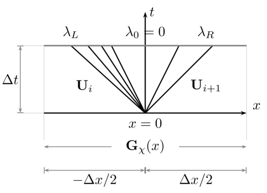
Figure 1. Integration control volume defined by a time interval $[0,\Delta t]$ and a space interval $[-\Delta x/2,\Delta x/2]$, with ${\lambda }_L$ $-\Delta x/2\le {\lambda }_L\Delta t$ and $\Delta x/2\ge {\lambda }_R\Delta t$, with ${\lambda }_L\ge {\lambda }_R$.

The source term is included in the Riemann solver as a singular source at the discontinuity point $x=0$ [33]. Considering that source terms are not necessarily constant over time, the following time linearization is applied [33,34]:

$${\mathbf{G}}_{i+1/2}=\frac{1}{\Delta t}{\int }_{-\Delta x/2}^{\Delta x/2}{\int }_0^{\Delta t}{\mathbf{G}}_{\chi }dxdt\approx {\left[\begin{array}{c}0\\ -\frac{\mathcal{A}}{\rho }(\delta p+g\rho \delta \eta )-\frac{\tilde{f}}{\rho }\Delta x\end{array}\right]}_{i+1/2},$$

(25)

with $\mathcal{A}$ a suitable value of vessel area defined depending on the flow conditions [28] and $\tilde{f}$ the integral of the friction force in the control volume. Using a discrete approach of the speed at the cell edge, ${\tilde{c}}_{i+1/2}$ [28], the discrete source term ${\mathbf{G}}_{i+1/2}$ can be expressed as:

$${\mathbf{G}}_{i+1/2}=-{\tilde{\mathbf{B}}}_{i+1/2}\delta {\mathbf{U}}_{i+1/2}+{\mathbf{S}}_{i+1/2},$$

(26)

with

$${\tilde{\mathbf{B}}}_{2,i+1/2}={\left[\begin{array}{cc}0& 0\\ {\tilde{c}}^2& 0\end{array}\right]}_{i+1/2},{\mathbf{S}}_{i+1/2}={\left[\begin{array}{c}0\\ -\frac{\mathcal{A}}{\rho }\delta p_d+{\tilde{c}}^2\delta A-\frac{\tilde{f}\Delta x}{\rho }\end{array}\right]}_{i+1/2},$$

(27)

with $p_d=p+g\rho \eta$ an equivalent pressure generated by the combination of the pressure and the gravitational force. The integral of the solution in the volume of interest in (22) is written as:

$${\int }_{-\Delta x/2}^{+\Delta x/2}\mathbf{U}(x,\Delta t)dx=\frac{\Delta x}{2}\left({\mathbf{U}}_i+{\mathbf{U}}_{i+1}\right)-\delta {\mathbf{M}}_{i+1/2}\Delta t,$$

(28)

with

$$\delta {\mathbf{M}}_{i+\frac{1}{2}}={(\delta \mathcal{F}-\mathbf{G})}_{i+\frac{1}{2}}={\tilde{\mathbf{J}}}_{i+\frac{1}{2}}\delta {\mathbf{U}}_{i+\frac{1}{2}}-{\mathbf{S}}_{i+\frac{1}{2}},{\tilde{\mathbf{J}}}_{i+\frac{1}{2}}={(\tilde{\mathbf{A}}+\tilde{\mathbf{B}})}_{i+\frac{1}{2}}.$$

(29)

Matrix $\tilde{\mathbf{J}}$ is a local matrix that provides a set of two real eigenvalues ${\tilde{\lambda }}^1=\tilde{u}-\tilde{c}$ and ${\tilde{\lambda }}^2=\tilde{u}+\tilde{c}$ with ${\tilde{\lambda }}_{i+\frac{1}{2}}^1<{\tilde{\lambda }}_{i+\frac{1}{2}}^2$, and two eigenvectors:

$${\tilde{\mathbf{e}}}_{i+1/2}^{1,2}={\left(1,{\tilde{\lambda }}^{1,2}\right)}_{i+1/2}^T,$$

(30)

and can be presented as the discrete Jacobian matrix of a flux function ${\hat{\mathbf{F}}}_e$ defined at each edge or interface between cells, that satisfies:

$$\delta {\hat{\mathbf{F}}}_{e,i+\frac{1}{2}}={\hat{\mathbf{F}}}_{e,i+1}-{\hat{\mathbf{F}}}_{e,i}={\tilde{\mathbf{J}}}_{i+\frac{1}{2}}\delta {\mathbf{U}}_{i+\frac{1}{2}}.$$

(31)

Under this condition, the following approximate semi-discrete RP in conservation-law form is presented [28]:

$$\frac{\partial \hat{\mathbf{U}}}{\partial t}+\frac{\delta {\hat{\mathbf{F}}}_e\left(\hat{\mathbf{U}}\right)}{\Delta x}=\frac{1}{\Delta x}{\mathbf{S}}_{i+\frac{1}{2}},\hat{\mathbf{U}}(x,0)=\left\{\begin{array}{ccc}{\mathbf{U}}_i& if& x<0\\ {\mathbf{U}}_{i+1}& if& x>0\end{array}\right.$$

(32)

where the new flux function ${\hat{\mathbf{F}}}_e$ is defined at each side of the RP as follows:

$$\begin{array}{c}{\hat{\mathbf{F}}}_{e,i}={\hat{\mathbf{F}}}_e\left({\mathbf{U}}_i\right)=\mathcal{F}\left({\mathbf{U}}_i\right)+{\tilde{\mathbf{B}}}_{i+\frac{1}{2}}{\mathbf{U}}_i,\\ \\ {\hat{\mathbf{F}}}_{e,i+1}={\hat{\mathbf{F}}}_e\left({\mathbf{U}}_{i+1}\right)=\mathcal{F}\left({\mathbf{U}}_{i+1}\right)+{\tilde{\mathbf{B}}}_{i+\frac{1}{2}}{\mathbf{U}}_{i+1},\end{array}$$

(33)

allowing us to define the fluctuations as:

$$\delta {\mathbf{M}}_{i+\frac{1}{2}}=\delta {\hat{\mathbf{F}}}_{e,i+\frac{1}{2}}-{\overline{\mathbf{S}}}_{i+\frac{1}{2}},$$

(34)

involving a flux difference and a source term.

2.2.2. The HLLS Solver

The HLLS method can be formulated by appropriately imposing the Rankine-Hugoniot (RH) conditions over the slowest (${\lambda }_L$) and fastest (${\lambda }_R$) wave celerities of the RP in (32), and the RH relation for the steady contact wave, of speed ${\lambda }_0=0$, at $x=0$, leading to the evolved fluxes ${\hat{\mathbf{F}}}_{e,i}^{-}$ and ${\hat{\mathbf{F}}}_{e,i+1}^{+}$ at the left and the right sides of the RP [27,28]:

$${\displaystyle {\hat{\mathbf{F}}}_{e,i+1}^{+}={\hat{\mathbf{F}}}_{e,i+1/2}^{\downarrow }+\frac{{\lambda }_R({\mathbf{S}}_{i+\frac{1}{2}}-{\lambda }_L{\mathbf{H}}_{i+\frac{1}{2}})}{{\lambda }_R-{\lambda }_L},{\hat{\mathbf{F}}}_{e,i}^{-}={\hat{\mathbf{F}}}_{e,i+1/2}^{\downarrow }+\frac{{\lambda }_L({\mathbf{S}}_{i+\frac{1}{2}}-{\lambda }_R{\mathbf{H}}_{i+\frac{1}{2}})}{{\lambda }_R-{\lambda }_L},}$$

(35)

with

$${\hat{\mathbf{F}}}_{e,i+1/2}^{\downarrow }=\frac{{\lambda }_R{\hat{\mathbf{F}}}_{e,i}-{\lambda }_L{\hat{\mathbf{F}}}_{e,i+1}+{\lambda }_L{\lambda }_R\delta {\mathbf{U}}_{i+\frac{1}{2}}}{{\lambda }_R-{\lambda }_L},{\mathbf{H}}_{i+1/2}={\tilde{\mathbf{J}}}_{i+\frac{1}{2}}^{-1}{\mathbf{S}}_{i+\frac{1}{2}}.$$

(36)

In order to allow variations in the geometrical and mechanical properties of the vessel, the inter-cell fluxes ${\mathbf{F}}_{i+\frac{1}{2}}^{\pm }$ in the approximate Godunov method in (15) are given by a combination of functions ${\hat{\mathbf{F}}}_e$ and ${\mathbf{F}}_{\phi }$:

$$\begin{array}{c}{\mathbf{F}}_{i+\frac{1}{2}}^{-}=({\hat{\mathbf{F}}}_{e,i}^{-}-{\hat{\mathbf{F}}}_i)+{\mathbf{F}}_{\phi ,i}=\delta {\mathbf{M}}_{i+\frac{1}{2}}^{-}+{\mathbf{F}}_{\phi ,i},\\ {\mathbf{F}}_{i+\frac{1}{2}}^{+}=({\hat{\mathbf{F}}}_{e,i+1}^{+}-{\hat{\mathbf{F}}}_{i+1})+{\mathbf{F}}_{\phi ,i+1}=-\delta {\mathbf{M}}_{i+\frac{1}{2}}^{+}+{\mathbf{F}}_{\phi ,i+1},\end{array}$$

(37)

leading to:

$${\mathbf{F}}_{i+1/2}^{-}=\left\{\begin{array}{ccc}{\mathbf{F}}_{\phi ,i}& if& 0\le {\lambda }_L\\ ({\hat{\mathbf{F}}}_{e,i+1/2}^{\downarrow }-{\hat{\mathbf{F}}}_{e,i})+\frac{{\lambda }_L({\mathbf{S}}_{i+1/2}-{\lambda }_R{\mathbf{H}}_{i+1/2})}{{\lambda }_R-{\lambda }_L}+{\mathbf{F}}_{\phi ,i}& if& {\lambda }_L\le 0\le {\lambda }_R\\ \delta {\hat{\mathbf{F}}}_{e,i+\frac{1}{2}}-{\mathbf{S}}_{i+1/2}+{\mathbf{F}}_{\phi ,i}& if& 0\ge {\lambda }_R\end{array}\right.,$$

(38)

$${\mathbf{F}}_{i+1/2}^{+}=\left\{\begin{array}{ccc}-(\delta {\hat{\mathbf{F}}}_{e,i+\frac{1}{2}}-{\mathbf{S}}_{i+1/2}+{\mathbf{F}}_{\phi ,i+1})& if& 0\le {\lambda }_L\\ ({\hat{\mathbf{F}}}_{e,i+1/2}^{\downarrow }-{\hat{\mathbf{F}}}_{e,i+1})+\frac{{\lambda }_R({\mathbf{S}}_{i+1/2}-{\lambda }_L{\mathbf{H}}_{i+1/2})}{{\lambda }_R-{\lambda }_L}+{\mathbf{F}}_{\phi ,i+1}& if& {\lambda }_L\le 0\le {\lambda }_R\\ {\mathbf{F}}_{\phi ,i+1}& if& 0\ge {\lambda }_R\end{array}\right..$$

(39)

In order to generate the intercell fluxes, it is necessary to compute the speeds ${\lambda }_R$ and ${\lambda }_L$. Suitable approximations of ${\lambda }_R$ and ${\lambda }_L$ are discussed in [27,28]. Their analysis is not the focus of the present work.

2.3. External Boundary Conditions at the Inflow-Outflow Sections of the Network

The definition of external boundary conditions for flow at the inlet or outlet sections in single vessels is necessary prior the generalization to junctions for merging flows, splitting flows or other possible combinations in a confluence of vessels. In this section, we will focus on the resolution of the evolved state ${\mathbf{U}}_k^{★}$ and its limits when defining boundary flow conditions ${\mathbf{U}}_k^{★}=[A_k^{★},Q_k^{★}]$. Assuming an imposed discharge at the boundary $[A_k^{★},Q_{bc}\left(t\right)]$. The following auxiliary function is defined depending on the position of the boundary cell [24]:

$$g_k\left(I_k\right)=\left\{\begin{array}{cc}\hfill 1,& if{I}_k=N_k\hfill \\ \hfill -1,& if{I}_k=1.\hfill \end{array}\right.$$

(40)

We will distinguish between outflow sections, where flow at the boundary cell leaves the domain, ${\left(gu\right)}_k^n>0$, and inflow sections, where flow initially enters at the boundary cell, ${\left(gu\right)}_k^n<0$. We also define the following boundary Speed Index (SI):

$$S{I}_g=g_k\frac{u_k}{c_k}.$$

(41)

where when $\left|S{I}_g\right|<1$ subsonic flow conditions will be defined.

2.3.1. Non-Linear Waves: Shocks and Rarefactions

For any boundary cell, and depending on the sign of the jump between the evolved state and the initial state for $\alpha$, $d{\alpha }_k={\alpha }_k^{★}-{\alpha }_k^n$, the solution will be a shock if $d{\alpha }_k>0$, or a rarefaction if $d{\alpha }_k<0$ [24,25]. To analyze the cases of interest and the possible limits, we define the celerities of the system as ${\lambda }_{1g}=u_k-g_k{c}_k$ and ${\lambda }_{2g}=u_k+g_k{c}_k$. As the solutions can only be developed in the inner region of each vessel, we will only need to explore solutions where $g_k{\lambda }_{1g}^{★}\le 0$, as shown in Figure 2 and Figure 3, where wave patterns for rarefactions and shocks are plotted, respectively. Solutions will be analyzed considering whether they take place in an outflow or inflow section.

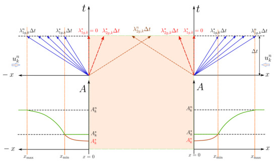
Figure 2. Rarefaction waves connecting the data state ${\mathbf{U}}_k^n$ with the evolved state ${\mathbf{U}}_k^{★}$ at the boundaries.

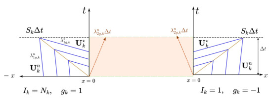
Figure 3. Shock waves connecting the data state ${\mathbf{U}}_k^n$ with the evolved state ${\mathbf{U}}_k^{★}$ at the boundaries.

• In the case of a rarefaction in a k vessel, the solution is given by the characteristic field [24,25],

  $$\frac{d{\alpha }_k}{1}=\frac{1}{A_{o,k}}\frac{d{Q}_k}{{\lambda }_{1g,k}},$$

  (42)

  and the jump condition across the rarefaction in invariant form becomes:

  $${\displaystyle u_k^{★}-u_k^n+g_k\delta W_k^{★}=0,\delta W^{★}={\int }_{{\alpha }^n}^{{\alpha }^{★}}\frac{c\left(a\right)}{a}da,}$$

  (43)

  with the following entropy condition:

  $$g_k{\lambda }_{1g,k}^n<g_k{\lambda }_{1g,k}^{★}\le 0.$$

  (44)
  Considering that along the rarefaction waves the vessel area decreases, the equation in (42) can be written as

  $$d{\alpha }_k=-{\left(\frac{1}{A_o\left|{\lambda }_{1g}\right|}\right)}_k{\left(gdQ\right)}_k<0,$$

  (45)

  or written as

  $$d{\alpha }_k=-{\left(\frac{\alpha }{c}\right)}_k{\left(gdu\right)}_k<0,$$

  (46)

  if expressed using variations in u. Both results suggest that velocity and flow variations must ensure:

  $${\left(gdu\right)}_k>0,{\left(gdQ\right)}_k>0,$$

  (47)

  and, therefore, during the suction produced by a decompression wave, the vessel area decreases while flow and velocity increased/decreased for backward/forward waves, respectively.
• If the solution in a k vessel is a shock of celerity S, that will travel in the $-g_{k}x$ direction, the Rankine–Hugoniot (RH) condition provides the solution. Solutions for right and left traveling shock waves can be defined using the following function [24,25]:

  $$u_k^{★}-u_k^n+g_k{f}_g^{★}=0,$$

  (48)

  with

  $$f_{g,k}^{★}={\left(\frac{1}{A_o}\left(\frac{1}{{\alpha }^n}-\frac{1}{{\alpha }^{★}}\right)\left({\phi }^{★}-{\phi }^n\right)\right)}_k^{\frac{1}{2}},$$

  (49)

  where the shock speed $S_k$ is given by:

  $$S_k=u_k^n-g{\left(\frac{{\phi }^{★}-{\phi }^n}{f_g^{★}{A}^n}\right)}_k,-g_k{S}_k>0,$$

  (50)

  under the following entropy conditions:

  $$g_k{\lambda }_{1g,k}^{★}<g_k{S}_k<g_k{\lambda }_{1g,k}^n.$$

  (51)
  The RH condition applied to the mass conservation equation in combination with the direction of the advance of the shock or compression wave, leads to the following expression:

  $$-g_{k}d{Q}_k=\left|S_k\right|A_{o,k}d{\alpha }_k>0,$$

  (52)

  and considering that $f_g>0$ in (48), we find that in boundary cells,

  $$-g_{k}d{u}_k=f_g>0.$$

  (53)
  Therefore, velocity and flow variations must ensure:

  $${\left(gdu\right)}_k<0,{\left(gdQ\right)}_k<0,$$

  (54)

  and for compression waves, the vessel area increases while flow and velocity are decreased/increased for backward/forward waves, respectively.

2.3.2. Pulse Wave Velocity in Arteries and Veins

The parameters m and n in the dimensionless transmural pressure difference $\sigma$ are different in arteries and veins and have an impact on the variation of the pulse wave velocity with the vessel deformation. Figure 4 shows the variation of the dimensionless PWV, $c/c_o$, versus the vessel deformation $\alpha$. While dimensionless PWV for arteries is a monotonically increasing function, dimensionless PWV for veins is a convex function with a minimum value of ${\alpha }_{min}={\left(n/m\right)}^{2/\left(m-n\right)}\approx 0.72$. This property has an interesting effect when observing the evolution of the solution for the $SI$ in a rarefaction in veins, when the jump in the vessel deformation $\alpha$ includes ${\alpha }_{min}$. In this case, the maximum value of the $SI$ appears when $\alpha ={\alpha }_{min}$ as shown in Figure 5.

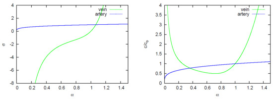
Figure 4. Dimensionless transmural pressure difference $\sigma$ (left) and dimensionless PWV, $c/c_o$, (right) versus the vessel deformation $\alpha$ for arteries and veins.

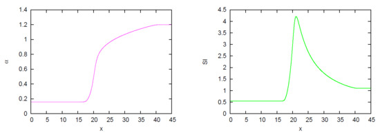
Figure 5. Solution of a right moving rarefaction wave with ${\alpha }^{★}<{\alpha }_{min}<{\alpha }_R$ in a vein (left). The maximum value of $SI$ appears when $\alpha ={\alpha }_{min}$ (right). Vessel properties are defined by $d_o=30.500$ cm and $c_o=118.72$ cm/s.

2.3.3. Outflow and Inflow Boundary Conditions in the Subsonic Flow Regime

For any boundary cell, the solution in the subsonic flow regime is defined by the solution of the non-linear waves (conservation of the invariant in (42) for rarefactions and the RH condition in (48) for shocks) together with mass conservation at the boundary cells:

$$\mathbf{E}\left(\mathbf{X}\right)=0,$$

(55)

with

$$\mathbf{E}\left(\mathbf{X}\right)=\left[\begin{array}{c}{u}^{★}-u^n+g\mathcal{B}\\ g{\alpha }^{★}{u}^{★}{A}_o-g{Q}_{bc}\end{array}\right],\mathbf{X}=\left[\begin{array}{c}{u}^{★}\\ {\alpha }^{★},\end{array}\right]$$

(56)

and

$$\mathcal{B}=\left\{\begin{array}{ccc}d{W}^{★}& if& \delta \alpha \le 0\\ f_g^{★}& if& \delta \alpha >0,\end{array}\right.$$

(57)

only valid under subsonic flow conditions.

The system of equations in (55) is non-linear and is solved here using Picard iterations between times t and $t+\Delta t$. In terms of notation, iterations are denoted by superscript m. The solution at m iteration or the initial solution ${\mathbf{X}}^m$ will be updated as follows:

$${\mathbf{X}}^{m+1}={\mathbf{X}}^m+\delta {\mathbf{X}}^m.$$

(58)

In order to find $\delta {\mathbf{X}}^m$, we first consider the Taylor expansions of the functions in $\mathbf{E}\left(\mathbf{X}\right)$. If the error terms $O_i\left(\delta {\mathbf{X}}^2\right)$ are assumed to be negligible, the system of equations can be written as follows:

$$\mathbf{E}\left({\mathbf{X}}^{m+1}\right)=\mathbf{E}\left({\mathbf{X}}^m\right)+{\mathbf{J}}_{\mathbf{E}}\left({\mathbf{X}}^m\right)\delta {\mathbf{X}}^m,$$

(59)

where ${\mathbf{J}}_{\mathbf{E}}\left(\mathbf{X}\right)$ is an $N_x\times N_x$ Jacobian matrix defined over the function vector $\mathbf{E}\left(\mathbf{X}\right)$. Now, all equations are expressed in linear form, and $\mathbf{E}\left({\mathbf{X}}^{m+1}\right)=0$ is imposed and $\delta {\mathbf{X}}^m$ is found to solve the equation

$${\mathbf{J}}_{\mathbf{E}}\left({\mathbf{X}}^m\right)\delta {\mathbf{X}}^m=-\mathbf{E}\left({\mathbf{X}}^m\right).$$

(60)

The system of equations in (60) can be solved using the Gauss–Jordan elimination method, and $\delta {\mathbf{X}}^{m+1}$ is obtained. Once all variables are updated, we can check if the new numerical error in ${\mathbf{E}}^{m+1}$ is under a desired tolerance. Otherwise, the procedure is repeated.

2.3.4. Limitation of Boundary Conditions at Outflow Sections

Considering that we are interested in imposing boundary flow conditions $Q_{bc}\left(t\right)$ at boundary cells, it is useful to define the limits in the variations in the jump in flow ${\left(g(Q^{★}-Q^n)\right)}_k$, depending on the resulting wave and on the initial flow conditions, subsonic or supersonic. In this section, we first analyze the solutions when imposing outflow boundary conditions, with $g_k{u}^n>0$.

• Case A1. Decompression waves under initial subsonic conditions, $0<S{I}_g^n<1$ (Figure 6).
  

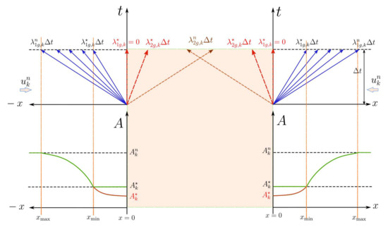  Figure 6. Case A1. Flow acceleration/deceleration at an outflow boundary condition generated by a backward/forward rarefaction wave. Initial subsonic state. In this outflow section a rarefaction wave evolves from $x_{max}={\lambda }_{1g}^n\Delta t$ to $x_{min}={\lambda }_{1g}^{★}\Delta t$. Rarefaction is limited by ${\lambda }_{1g}^{★}=0$ or $x_{min}=0$.
  Suction is generated in the outflow section and a rarefaction or decompression wave appears according to (47). The value of the $S{I}_g$ increases in the $g_{k}x$ direction with $\left|u^{★}\right|>\left|u^n\right|$. As the solution can be only developed in the inner region of the vessel, $g{\lambda }_{1g}^{★}\le 0$, the value of the speed index at the boundary, $S{I}_g^{★}$, must be limited to conditions of sonic flow:

  $$S{I}_g^{★}=\frac{g_k{u}^{★}}{c^{★}}=\frac{\left|u^{★}\right|}{c^{★}}\le 1.$$

  (61)
  Therefore, a critical limit in the velocity and flow, $u_c$ and $Q_c$, appears when imposing the boundary condition:

  $$g{Q}_{bc}\le g{Q}_c,Q_c={\left(u_c{\alpha }^{★}{A}_o\right)}_k,u_{c,k}=g_k{c}_k^{★}.$$

  (62)
  Then, if the limit in (61) is exceeded, the solution is given by the function $F_1\left(\alpha \right):$

  $${\displaystyle F_1\left(\alpha \right)=g_k{c}_k-u_k^n+g_k\delta W_k^{★},}$$

  (63)

  and the solution for flow is given by $Q_{bc}=Q^{★}=Q_c$.
• Case A2. Decompression waves under initial supersonic conditions, $S{I}_g^n>1$ (Figure 7).
  

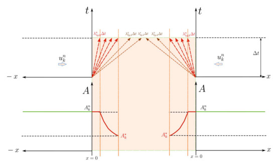  Figure 7. Case A2. Flow acceleration/deceleration at an outflow boundary condition. Initial supersonic state. In this outflow section both ${\lambda }_{1g}^n$ and ${\lambda }_{2g}^n$ waves fall outside the computational domain. The solution can not evolve inside the vessel.
  For a supersonic initial state, both celerities ${\lambda }_{1g}$ and ${\lambda }_{2g}$ fall outside the domain of computation and the limit in (61) has already been exceeded. Further acceleration/deceleration would mean to force the development of the solution outside the vessel. Under these conditions no information can travel inside the domain and the initial state cannot change. We cannot specify any boundary conditions [35].
• Case B1. Compression waves under initial subsonic conditions, $0<S{I}_g^n<1$ (Figure 8).
  

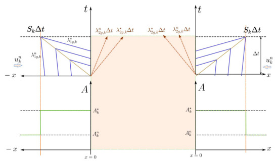  Figure 8. Case B1. Flow deceleration/acceleration generated by a backward/forward shock wave at an outflow boundary condition. Initial subsonic state. The solution satisfies $\left|{\lambda }_{1g}^{★}\right|>\left|{\lambda }_{1g}^n\right|$.
  When the flow is decelerated/accelerated at the boundary in presence of backward/forward wave, the vessel area increases. The value of the $S{I}_g$ decreases in the $g_{k}x$ direction and sonic conditions cannot be achieved.
• Case B2. Compression waves under initial supersonic conditions, $S{I}_g^n>1$ (Figure 9). For a supersonic initial state, the wave ${\lambda }_{1g}^n$ falls outside the computational domain. When the flow is decelerated at the boundary, the shock must satisfy the entropy condition in (51), ensuring $g{\lambda }_{1g}^{★}<0$. Therefore, sonic conditions cannot be achieved.
  

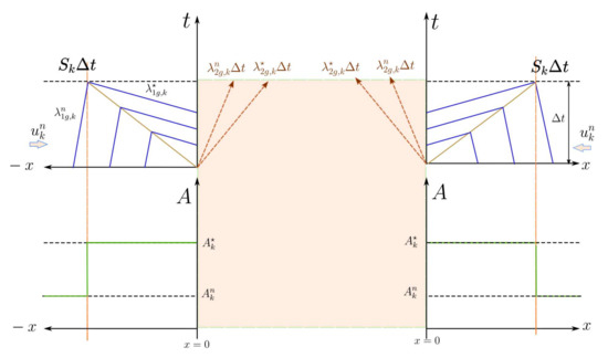  Figure 9. Case B2. Flow deceleration/acceleration generated by a backward/forward shock wave at an outflow boundary condition. Initial supersonic state. A shock wave moving inside the domain is generated if the imposed boundary condition is able to ensure $g{\lambda }_{1g}^{★}\le 0$ departing form $g{\lambda }_{1g}^n>0$.

2.3.5. Limitation of Boundary Conditions at Inflow Sections

In this section, we analyze the limits and constrains that appear in presence of backward and forward compression or decompression waves for inflow sections with $g_k{u}^n<0$. We define the following cases.

• Case C1. Compression waves under initial subsonic conditions, $-1<S{I}_g^n<0$ (Figure 10).
  

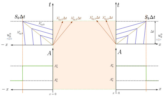  Figure 10. Case C1. Flow deceleration/acceleration, $g_{k}d{Q}_{bc}<0$, at an inflow boundary condition under initial subsonic conditions. In this inflow section a backward/forward shock wave moving inside the domain is generated.
  Under these conditions, the vessel area increases $d\alpha >0$ and the solution is a shock or compression wave moving in the $-g_{k}x$ direction, where $\left|{\lambda }_{1g,k}^{★}\right|>\left|{\lambda }_{1g,k}^n\right|$.
• Case C2. Compression waves under initial supersonic conditions, $S{I}_g^n<-1$ (Figure 11).
  

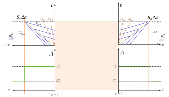  Figure 11. Case C2. Flow deceleration/acceleration, $g_{k}d{Q}_{bc}<0$, at an inflow boundary condition under initial supersonic conditions. In this inflow section a backward/forward shock wave moving inside the domain is generated. Both ${\lambda }_{1g}^n$ and ${\lambda }_{2g}^n$ fall inside of the domain. Two boundary conditions are required.
  In the supersonic range, both ${\lambda }_{1g}^n$ and ${\lambda }_{2g}^n$ fall inside the domain. Apart from the prescribed flow, another condition, such as vessel area or total energy must be imposed. Initial conditions and boundary conditions may satisfy the relation in (51) and entropy conditions in (48).
• Case D1. Decompression waves under initial subsonic conditions, $-1<S{I}_g^n<0$ (Figure 12).
  

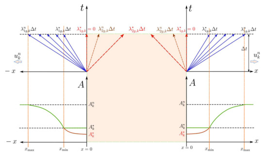  Figure 12. Case D1. Flow acceleration/deceleration, $g_{k}d{Q}_{bc}>0$, at an inflow boundary condition under initial subsonic conditions. In this inflow section a backward/forward rarefaction wave appears. The solution evolves from $x_{max}={\lambda }_{1g}^n\Delta t$ to $x_{min}={\lambda }_{1g}^{★}\Delta t$. When ${\lambda }_{1g}^{★}=0$ the flow velocity direction is opposite to the initial one.
  In the subsonic range, we find that $\left|u^{★}\right|<\left|u^n\right|$. The limiting value of $Q_{bc}$ is given by $g_k{\lambda }_{1g}^{★}=0$, or $g_k{u}^{★}=c^{★}$, and represents a condition of reversal flow. When this limit is exceeded, sonic conditions must be imposed, and the solution is given by function in (63).
• Case D2. Decompression waves under initial supersonic conditions, $S{I}_g^n<-1$ (Figure 13).
  

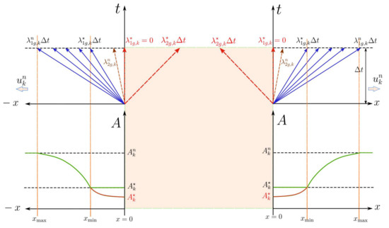  Figure 13. Case D2. Flow acceleration/deceleration, $g_{k}d{Q}_{bc}>0$, at an inflow boundary condition under initial supersonic conditions. In this inflow section a backward/forward rarefaction wave can defined inside the domain as ${\lambda }_{1g}^n$ falls within the domain. When ${\lambda }_{1g}^{★}=0$ the flow velocity direction is opposite to the initial one.
  Again, the limiting state, a condition of reversal flow, is provided by $g_k{\lambda }_{1g}^{★}=0$ and, if exceeded, the solution is given by function in (63).

2.3.6. Outflow and Inflow Boundary Conditions including Subsonic, Sonic and Supersonic Flow

The previous cases in Section 2.3.4 and Section 2.3.5 can be reorganized depending on the initial flow regime. For subsonic flow, $\left|S{I}_g^n\right|<1$, we find that:

• If $0<S{I}_g^n<1$, at outflow boundary conditions:
  • The acceleration/deceleration of the flow generated by a backward/forward wave can be imposed provided that the limiting value of flow in (62) is not exceeded, leading to a decompression wave (case A1).
  • The deceleration/acceleration of the flow generated by a backward/forward wave can be imposed leading to a compression wave (case B1), and no sonic limitation appears.
• If $-1<S{I}_g^n<0$, at inflow boundary conditions:
  • Flow deceleration/acceleration, generated by a backward/forward wave can be imposed leading to a compression wave (case C1).
  • Flow acceleration/deceleration, generated by a backward/forward wave leads to a decompression wave. Flow at the boundary must by limited by the function in (63) (case D1).

For supersonic flow:

• If $S{I}_g^n>1$, at outflow boundary conditions:
  • The acceleration/deceleration of the flow cannot be imposed, as no information can arrive to the inner domain of the vessel (case A2), ${\mathbf{U}}_k^{★}={[A^n,Q^n]}_k^T$.
  • The deceleration/acceleration of the flow, generated by a backward/forward wave can be imposed if leading to a compression wave with a suitable value of celerity (case B2), $-g_{k}S>0$.
• If $S{I}_g^n<-1$, in inflow boundary conditions:
  • The deceleration/acceleration of the flow generated by a backward/forward wave can be imposed, leading to a compression wave, provided that both flow and area are imposed (case C2), ${\mathbf{U}}_k^{★}={[A_{bc}\left(t\right),Q_{bc}\left(t\right)]}_k^T$.
  • The deceleration of the flow can be imposed, leading to a decompression wave (case D2) limited by the function in (63).

Therefore, we need to provide solutions considering that:

• The target functions in system (55) must be redefined to ensure limitation of sonic flow in cases A1, D1 y D2.
• Unfeasible acceleration/deceleration, in supersonic outflow sections in case A2 must be avoided, the target functions in system (55) must be redefined to include this case.
• In case C2, involving a supersonic inflow section, both area and flow rate must be imposed. In this case, the system of equations in (55) is useless.

In order to limit the possible transitions, the system of equations in (55) is modified. Now, error function in (55) is written as the sum of two functions:

$$\mathbf{E}\left(\mathbf{X}\right)={\mathbf{E}}^a\left(\mathbf{X}\right)+{\mathbf{E}}^b\left(\mathbf{X}\right)=0,$$

(64)

with

$${\mathbf{E}}^a\left(\mathbf{X}\right)=\left[\begin{array}{c}{(u^{•}-u^n+g\mathcal{B})}_k{\mathcal{D}}_{w,k}\\ {\left[g{\mathcal{D}}_w\left({\alpha }^{★}{A}_o{u}^{•}\right)+g(1-{\mathcal{D}}_w)Q^n\right]}_k-g_k{Q}_{bc,k}^{•}\end{array}\right],{\mathbf{E}}^b\left(\mathbf{X}\right)=\left[\begin{array}{c}{(u^{★}-u^n)}_k(1-{\mathcal{D}}_{w,k})\\ {({\alpha }^{★}-{\alpha }^n)}_k(1-{\mathcal{D}}_{w,k})\end{array}\right].$$

(65)

The first equation in (65), accounting for the solution of non-linear waves, involves the following velocity

$$u_k^{•}={\mathcal{R}}_{w,k}{g}_k{c}_k^{★}+{\mathcal{T}}_w{u}_k^{★},{\mathcal{T}}_w=1-{\mathcal{R}}_w,$$

(66)

with

$${\mathcal{R}}_w=\left\{\begin{array}{ccccccc}\hfill 1& if& S{I}_g^{★,m}<1& \mathrm{and}& S{I}_g^{★,m+1}>1& \mathrm{and}& \delta {\alpha }^m\le 0\\ \hfill 0& \mathrm{otherwise},\end{array}\right.$$

(67)

and $\delta \alpha ={({\alpha }^{★}-{\alpha }^n)}_k$. ${\mathcal{T}}_w$ is zero when sonic conditions are reached during the iterative search of a rarefaction solution, resulting in ${\mathcal{R}}_w=1$. In this case, $u^{★}$ is no longer an unknown and the rarefaction waves remain limited by ${\lambda }_{1g}^{★}=0$.

The coefficient ${\mathcal{D}}_w$ retains the initial values for velocity and area for those outflow sections where supersonic conditions are initially defined (case A2) when necessary. ${\mathcal{D}}_w$ is defined as:

$${\mathcal{D}}_w=\left\{\begin{array}{cccc}\hfill 0& if& S{I}_g^n\ge 1\mathrm{and}& g_k{(Q_{bc}-Q^n)}_k>0\mathrm{or}{({\alpha }^{★}-{\alpha }^n)}_k<0\\ \hfill 0& if& S{I}_g^n\ge 1\mathrm{and}& -g_{k}S<0\\ \hfill 1& \mathrm{otherwise},\end{array}\right.$$

(68)

avoiding further acceleration of the flow in supersonic conditions or unphysical shock wave directions.

Mass conservation in the system of equations in (65) is defined using the following auxiliary variable

$$Q_{bc,k}^{•}={\left[{\mathcal{T}}_w{\mathcal{D}}_w{Q}_{bc,k}^m+{\mathcal{R}}_w{\mathcal{D}}_w\left({\alpha }^{★}{A}_o{u}^{•}\right)+(1-{\mathcal{D}}_w)Q^n\right]}_k,$$

(69)

leading to the initial value of discharge when ${\mathcal{D}}_w$ = 0, to conditions of sonic flow when ${\mathcal{R}}_w=1$ or to the objective value $Q_{bc,k}^m$ if subsonic conditions are retained, ${\mathcal{T}}_w{\mathcal{D}}_w=1$. The auxiliary flow value $Q_{bc}^m$ approximates $Q_{bc}\left(t\right)$ and ensures a smooth convergence to the solution, will be defined below.

Matrix ${\mathbf{J}}_{\mathbf{E}}\left(\mathbf{X}\right)={\mathbf{J}}_{\mathbf{E}}^a\left(\mathbf{X}\right)+{\mathbf{J}}_{\mathbf{E}}^b\left(\mathbf{X}\right)$, is given by:

$${\mathbf{J}}_{\mathbf{E}}^a\left(\mathbf{X}\right)=\left[\begin{array}{cc}{\mathcal{T}}_w{\mathcal{D}}_w& \left({\mathcal{R}}_{w}g\frac{\partial c}{\partial \alpha }+g\frac{\partial \mathcal{B}}{\partial \alpha }\right){\mathcal{D}}_w\\ \left({\mathcal{T}}_w{\mathcal{D}}_{w}g{A}_o\right){\alpha }^{★}& \left({\mathcal{T}}_w{\mathcal{D}}_{w}g{A}_o\right)u^{★}\end{array}\right],{\mathbf{J}}_{\mathbf{E}}^b\left(\mathbf{X}\right)=\left[\begin{array}{cc}1-{\mathcal{D}}_w& 0\\ (1-{\mathcal{T}}_w){\mathcal{D}}_w& 1-{\mathcal{D}}_w\end{array}\right],$$

(70)

with

$$\frac{\partial \mathcal{B}}{\partial \alpha }=\left\{\begin{array}{ccc}\frac{g{c}^{★}}{{\alpha }^{★}}& if& \delta \alpha \le 0\\ \frac{\partial f_g}{\partial \alpha }& if& \delta \alpha >0\end{array}\right.$$

(71)

and

$$\frac{\partial c}{\partial \alpha }=\frac{1}{2}\frac{c_o^2}{(m-n)}\frac{(m^2{\alpha }^m-n^2{\alpha }^n)}{c\alpha }\frac{\partial f_g}{\partial \alpha }=\frac{1}{2f_g}\left[\left(\frac{1}{{\alpha }^n}-\frac{1}{{\alpha }^{★}}\right){\left(c^{★}\right)}^2+\frac{1}{A_o}{\left(\frac{1}{{\alpha }^{★}}\right)}^2\left({\phi }^{★}-{\phi }^n\right)\right].$$

(72)

In this way, when sonic conditions are reached and $u^{★}$ is no longer an unknown, the numerical method presented here avoids the updating of $u^{★}$, setting $\delta u^{★}=0$.

Initial Values and Relaxation Parameters

In the first iteration, $m=0$, the solution will be defined assuming that:

• if $g(Q_{bc}-Q^n)\ge 0$, the solution will be a rarefaction,
• if $g(Q_{bc}-Q^n)<0$, the solution will be a shock.

In order to avoid an excessive variation of $\alpha$ between two steps, we reduce the step size $\delta {\mathbf{X}}^m$ by using a damping factor ${\gamma }_{\alpha }\le 1$:

$$\delta {\mathbf{X}}^m={\gamma }_{\alpha }\delta {\mathbf{X}}^m,{\gamma }_{\alpha }=\left\{\begin{array}{cc}1& if \left|\delta {\alpha }^m\right|<\delta {\alpha }_{lim}\hfill \\ \frac{\delta {\alpha }_{lim}}{\left|\delta {\alpha }^m\right|}& if \left|\delta {\alpha }^m\right|>\delta {\alpha }_{lim}\hfill \end{array}\right.,$$

(73)

with $\delta {\alpha }_{lim}$ a constant value, defined to limit the variation of $\alpha$.

Next, we also limit the variation in $\delta {\mathbf{X}}^m$ by imposing a constraint in the maximum variation of the velocity u, $\delta u_{lim}$, by using the damping factor ${\gamma }_u\le 1$.

$$\delta {\mathbf{X}}^m={\gamma }_u\delta {\mathbf{X}}^m,{\gamma }_u=\left\{\begin{array}{cc}1& if \left|\delta u^m\right|<\delta u_{lim}\hfill \\ \frac{\delta u_{lim}}{\left|\delta u^m\right|}& if \left|\delta u^m\right|>\delta u_{lim}\hfill \end{array}\right..$$

(74)

In this case, $\delta u_{lim}$ is not a fixed value as $\delta {\alpha }_{lim}$. The variation in $\delta u_{lim}$ is computed assuming that the increase in $S{I}_g$ from iteration m to $m+1$, $\left|\delta S{I}_g^m\right|=\left|S{I}_g^{m+1}-S{I}_g^m\right|$, is small and small enough to control the solution when the solution is in the vicinity of sonic flow conditions. This is ensured by limiting the increment $\left|\delta S{I}_g^m\right|$ by a prefixed constant value, $\delta S{I}_{lim}$, which can be also reduced to avoid sonic conditions when $\left|S{I}_g\right|=1$, as follows:

$$\left|\delta S{I}_g^m\right|=\left\{\begin{array}{cc}min(\delta S{I}_{lim},\left|1-\left|S{I}_g^m\right|\right|)& if 0\le S{I}_g^m<1\hfill \\ \delta S{I}_{lim}& \mathrm{otherwise}\hfill \end{array}\right..$$

(75)

With this value of $\left|\delta S{I}_g^m\right|$, the maximum variation of velocity is approximated by:

$$\delta u_{lim}=\left|\delta S{I}_g^m\right|c^m,$$

(76)

as small variations in $\alpha$ have been enforced. The final solution will also be achieved not directly imposing the value of $Q_{bc}$ in the mass conservation equation, but changing its value smoothly using the auxiliary variables $Q_{bc}^m$ and $\delta Q_{bc}^m$, with:

$$\delta Q_{bc}^m=\left\{\begin{array}{cc}\delta u_{lim}\left({\alpha }^m{A}_o\right)& if Q_{bc}-Q_{bc}^m>0\hfill \\ -\delta u_{lim}\left({\alpha }^m{A}_o\right)& if Q_{bc}-Q_{bc}^m<0,\hfill \end{array}\right.$$

(77)

untill the final solution for $Q_{bc}$ is achieved, with:

$$Q_{bc}^{m+1}=\left\{\begin{array}{cc}\hfill min\left(Q_{bc}^m+\delta Q_{bc}^m,Q_{bc}\right),& if\delta Q^m>0\hfill \\ \hfill max\left(Q_{bc}^m+\delta Q_{bc}^m,Q_{bc}\right),& if\delta Q^m<0\hfill \end{array}\right.$$

(78)

limiting the value of $Q_{bc}$ in the mass conservation equation when sonic conditions are reached. The details of the invariant integration are given in Appendix A.

2.4. Solution of the JRP

The Riemann problem at vertex P or JRP, for $N_P$ infinitely long converging vessels sharing vertex P reads:

$$\frac{\partial {\mathbf{U}}_k}{\partial t}+\mathbf{J}\left({\mathbf{U}}_k\right)\frac{\partial {\mathbf{U}}_k}{\partial x}=0,{\hat{\mathbf{U}}}_k(x,0)={\mathbf{U}}_{i,k},$$

(79)

for $k=1,\dots ,N_P$. To couple the $N_P$ vessels, we have to compute the unknown cross-sectional area $A_k^{★}$ and velocity $u_k^{★}$ for each vessel converging at node P, which means that we have $2N_P$ unknowns. Quantities $A_k^{★}$ and $u_k^{★}$ will be used to compute fluxes at the boundary interface of the k-th vessel. For the $N_P$ boundary cells meeting at the junction, the following mass conservation equation is written:

$$\sum _{k=1}^{N_P}{g}_k{Q}_k^{★}=0,$$

(80)

where $Q_k^{★}=u_k^{★}{A}_k^{★}$. The solution of the JRP under subsonic flow conditions is next revisited and later extended to general flow conditions.

2.4.1. Solution of the JRP under Subsonic Flow Conditions

The solution of the JRP under subsonic flow conditions can be defined by a system of $2N_P$ equations of the form $\mathbf{E}\left(\mathbf{X}\right)=0$. The first $N_P$ equations are relations for non-linear waves (conservation of the Riemann Invariants in (42) or shock waves in (48)). The remaining $N_P$ equations, mass conservation in (80) and the $N_P-1$ equations involving conservation of total pressure, $p_T$, are related to the stationary contact discontinuity generated by variable mechanical and geometrical properties [24]:

$$\mathbf{E}\left(\mathbf{X}\right)=\left[\begin{array}{c}{(u^{★}-u^n+g\mathcal{B})}_1\\ ⋮\\ {(u^{★}-u^n+g\mathcal{B})}_{N_P}\\ \sum _k{\left(g{\left(\alpha u\right)}^{★}{A}_o\right)}_k\\ p_{T,1}-p_{T,2}\\ ⋮\\ p_{T,1}-p_{T,N_P}\end{array}\right],\mathbf{X}=\left[\begin{array}{c}{u}_1^{★}\\ ⋮\\ u_{N_P}^{★}\\ {\alpha }_1^{★}\\ ⋮\\ {\alpha }_{N_P,}^{★}\end{array}\right]$$

(81)

with $p_T=p_M+K_o\sigma +\frac{1}{2}\rho u^2$, $p_M=p_o+p_{ext}+\rho g\eta$, and $\mathcal{B}$ defined in (57), where vessel $k=1$ is used to define the reference value in the energy conservation equation.

The system of equations in (81) can be linearized and solved using Picard iterations between times t and $t+\Delta t$, using a Jacobian matrix ${\mathbf{J}}_{\mathbf{E}}^m$ defined over the function vector $\mathbf{E}$, where $\delta {\mathbf{X}}^m$ is obtained. In this case, matrix ${\mathbf{J}}_{\mathbf{E}}$ is given by:

$${\mathbf{J}}_{\mathbf{E}}\left(\mathbf{X}\right)={\left[\begin{array}{cc}{\mathbf{J}}_{\mathbf{E},\mathbf{1}}& {\mathbf{J}}_{\mathbf{E},\mathbf{2}}\\ {\mathbf{J}}_{\mathbf{E},\mathbf{3}}& {\mathbf{J}}_{\mathbf{E},\mathbf{4}}\end{array}\right]}_{\left(2N_P\right)\times \left(2N_P\right)},$$

(82)

where

$${\mathbf{J}}_{\mathbf{E}},\mathbf{1}={\mathbf{I}}_{N_P\times N_P},{\mathbf{J}}_{\mathbf{E},\mathbf{2}}={\left[\begin{array}{ccc}{\left(g\frac{\partial \mathcal{B}}{\partial \alpha }\right)}_1& 0& 0\\ 0& \ddots & 0\\ 0& 0& {\left(g\frac{\partial \mathcal{B}}{\partial \alpha }\right)}_{N_P}\end{array}\right]}_{N_P\times N_P},$$

(83)

and

$${\mathbf{J}}_{\mathbf{E},\mathbf{3}}={\left[\begin{array}{cccc}{\left(g{\alpha }^{★}{A}_o\right)}_1& {\left(g{\alpha }^{★}{A}_o\right)}_2& \cdots & {\left(g{\alpha }^{★}{A}_o\right)}_{N_P}\\ {\left(K_o\frac{\partial \sigma }{\partial \alpha }\right)}_1& -{\left(K_o\frac{\partial \sigma }{\partial \alpha }\right)}_2& \cdots & 0\\ ⋮& 0& \ddots & 0\\ {\left(K_o\frac{\partial \sigma }{\partial \alpha }\right)}_1& 0& \cdots & -{\left(K_o\frac{\partial \sigma }{\partial \alpha }\right)}_{N_P}\end{array}\right]}_{N_P\times N_P},$$

(84)

$${\mathbf{J}}_{\mathbf{E},\mathbf{4}}={\left[\begin{array}{cccc}{\left(g{u}^{★}{A}_o\right)}_1& {\left(g{u}^{★}{A}_o\right)}_2& \cdots & {\left(g{u}^{★}{A}_o\right)}_{N_P}\\ \rho u_1^{★}& -\rho u_2^{★}& \cdots & 0\\ ⋮& 0& \ddots & 0\\ \rho u_1^{★}& 0& \cdots & -\rho u_{N_P}^{★}\end{array}\right]}_{N_P\times N_P},$$

(85)

with

$$\frac{\partial \sigma }{\partial \alpha }=\frac{K_o}{\alpha }[m{\alpha }^m-n{\alpha }^n].$$

(86)

2.4.2. Solution of the JRP under Subsonic and Supersonic Flow Conditions

The system of equations for subsonic flow conditions is modified here to deal with both subsonic and supersonic flow conditions. After each iteration, the variables of the system in $\mathbf{X}$ and a set of dynamic parameters for each vessel will be updated. The new system of equations is split into two terms:

$$\mathbf{E}\left(\mathbf{X}\right)={\mathbf{E}}^a\left(\mathbf{X}\right)+{\mathbf{E}}^b\left(\mathbf{X}\right)=0,$$

(87)

with

$${\mathbf{E}}^a=\left[\begin{array}{c}{(u^{•}-u^n+g\mathcal{B})}_1{\mathcal{D}}_{w,1}\\ ⋮\\ {(u^{•}-u^n+g\mathcal{B})}_{N_P}{\mathcal{D}}_{w,N_P}\\ \sum _k{\left[g{\mathcal{D}}_w\left({\alpha }^{★}{A}_o{u}^{•}\right)\right]}_k\\ \left[p_T^{★}-p_{T,2}\right]{\mathcal{Q}}_{w,2}\\ ⋮\\ \left[p_T^{★}-p_{T,N_P}\right]{\mathcal{Q}}_{w,N_P}\end{array}\right],{\mathbf{E}}^b=\left[\begin{array}{c}{(u^{★}-u^n)}_1(1-{\mathcal{D}}_{w,1})\\ ⋮\\ {(u^{★}-u^n)}_{N_P}(1-{\mathcal{D}}_{w,N_P})\\ \sum _k{g}_k{\left[(1-{\mathcal{D}}_w){\left(Au\right)}^n\right]}_k\\ {\displaystyle {({\alpha }^{★}-{\alpha }^n)}_1(1-{\mathcal{D}}_{w,1}){\mathcal{L}}_{w,2}+{({\alpha }^{★}-{\alpha }^n)}_2(1-{\mathcal{D}}_{w,2})}\\ ⋮\\ {\displaystyle {({\alpha }^{★}-{\alpha }^n)}_1(1-{\mathcal{D}}_{w,1}){\mathcal{L}}_{w,N_P}+{({\alpha }^{★}-{\alpha }^n)}_{N_P}(1-{\mathcal{D}}_{w,N_P}).}\end{array}\right].$$

(88)

${\mathbf{E}}^b\left(\mathbf{X}\right)$ is defined to impose conservation of the initial value conditions in a k vessel depending on the dynamic parameter ${\mathcal{D}}_{w,k}$. Parameter ${\mathcal{D}}_{w,k}$ is defined as follows:

$${\mathcal{D}}_w=\left\{\begin{array}{ccccc}\hfill 0& if& S{I}_g^n\ge 1& \mathrm{and}& g_k{(Q^{★}-Q^n)}_k>0\mathrm{or}{({\alpha }^{★}-{\alpha }^n)}_k<0\\ \hfill 0& if& S{I}_g^n\ge 1& \mathrm{and}& -g_{k}S<0\\ \hfill 0& if& S{I}_g^n\ge 1& \mathrm{and}& -g_k{\lambda }_{1g,k}^{★}<0\\ \hfill 1& \mathrm{otherwise}\end{array}\right..$$

(89)

It is worth noting that, for outflow sections under supersonic conditions, it becomes zero if the iterative solution leads to an unphysical solution. Unphysical solutions are associated with flow acceleration, to a reduction of the vessel area or to a shock wave traveling in the wrong direction (analogous to case A2 in the external boundary analysis). In this case, both the area and the velocity of the vessel are no longer an unknown of the system, and ${\mathbf{U}}_k^{★}={\mathbf{U}}_k^n$ must be enforced. On the other hand, when ${\mathcal{D}}_{w,k}=1$, the transmission of a backward wave generated downstream of a convergence point is guaranteed.

When coefficient ${\mathcal{D}}_{w,k}=1$, the error function $E_k$ for vessels $k=1,\cdots ,N_p$, reduces to $E_k^a$ accounting for relations across non-linear waves, involving the auxiliary variable $u^{•}$ in (66).

If sonic flow conditions are reached during the iterative process for vessel k, the evolved solution for the velocity is $g_k{c}^{★}$, and this velocity is no longer an unknown of the problem. When the parameter ${\mathcal{D}}_{w,k}=0$, the error function $E_k=E_k^b$, expressing that the initial condition for the velocity must be kept over time, $u_k^{★}=u_k^n$.

The definition of the velocity in (66) enables a generic formulation for the flow in a vessel as follows:

$$Q_k^{★}={\mathcal{D}}_{w,k}{\left({\alpha }^{★}{A}_o{u}^{•}\right)}_k+(1-{\mathcal{D}}_{w,k})Q_k^n,$$

(90)

and error function $E_{N_P+1}$ for mass conservation is split in $E_{N_P+1}^a$ and $E_{N_P+1}^b$ depending on the value of ${\mathcal{D}}_{w,k}$.

Error functions $E_{N_P+1+k}$ for $k=2,\dots ,N_p$ are modified to consider that the evolved state of a vessel may not participate in the energy conservation equation. The reference value in the energy conservation equation is:

$$p_T^{★}=\sum _{k=1}^{N_P}{\mathcal{L}}_{w,k}{p}_{T,k},$$

(91)

with

$${\mathcal{L}}_{w,k}=\left\{\begin{array}{ccc}1& if& k=k_{\mathcal{L}}\\ 0& \mathrm{otherwise}\end{array}\right.,k_{\mathcal{L}}=min\left\{k,{\mathcal{T}}_{w,k}{\mathcal{D}}_{k,w}=1\right\},k=1,\dots ,N_P.$$

(92)

Coefficient ${\mathcal{L}}_{w,k}$ is always zero except for in the first eligible vessel where energy conservation can be defined and this k vessel will be used as the reference value in the energy conservation equation. Ineligible vessels do not participate in the energy conservation equation when ${\mathcal{T}}_{w,k}=0$ (flow limitation) or ${\mathcal{D}}_w=0$ (conservation of the initial condition). Coefficient ${\mathcal{Q}}_{w,k}$ is defined as:

$${\mathcal{Q}}_{w,k}={\mathcal{T}}_{w,k}{\mathcal{D}}_{w,k}(1-{\mathcal{L}}_{w,k}),$$

(93)

and may become equal to 0 or 1. In the case that ${\mathcal{L}}_{w,k}=1$, ${\mathcal{Q}}_{w,k}$ becomes zero as this k vessel will be used as the reference value in the energy conservation equation. Coefficient ${\mathcal{Q}}_{w,k}$ also becomes zero when the flow reaches sonic conditions in a rarefaction or when the flow is supersonic and cannot be further accelerated with independence of the gradient of energy across the junction. In both cases, these ineligible vessels do not participate in energy conservation equation, as their solution becomes independent of the energy level of the other vessels.

When for $k>1$, ${\mathcal{D}}_{w,k}=0$, the energy conservation equation in $E_{N_P+1+k}^a$ is omitted and preservation of initial conditions for vessel area, ${\alpha }_k^{★}={\alpha }_k^n$, is enforced in $E_{N_P+1+k}^b$. When ${\mathcal{D}}_{w,1}=0$, ${\alpha }_1^{★}={\alpha }_1^n$ is imposed in error function $E_{N_P+1+k}^b$, with k the first eligible vessel with ${\mathcal{L}}_{w,k}=1$. This k vessel does not require further equations as it has already been used to provide the energy reference level.

System of equations in (87) is indirectly solved using the equivalent linear system in (60), where Jacobian matrix ${\mathbf{J}}_{\mathbf{E}}\left(\mathbf{X}\right)$ is defined as:

$${\mathbf{J}}_{\mathbf{E}}\left(\mathbf{X}\right)={\left[\begin{array}{cc}{\mathbf{J}}_{\mathbf{E},\mathbf{1}}& {\mathbf{J}}_{\mathbf{E},\mathbf{2}}\\ {\mathbf{J}}_{\mathbf{E},\mathbf{3}}& {\mathbf{J}}_{\mathbf{E},\mathbf{4}}\end{array}\right]}_{\left(2N_P\right)\times \left(2N_P\right)}=\left[\begin{array}{ccc}{e}_{1,1}& \cdots & e_{1,2N_P}\\ ⋮& \ddots & ⋮\\ e_{2N_P,1}& \cdots & e_{2N_P,2N_P},\end{array}\right]$$

(94)

and matrices ${\mathbf{J}}_{\mathbf{E}},\mathbf{1}$ and ${\mathbf{J}}_{\mathbf{E}},\mathbf{2}$ involve relations for non-linear waves and matrices ${\mathbf{J}}_{\mathbf{E}},\mathbf{3}$ and ${\mathbf{J}}_{\mathbf{E}},\mathbf{4}$ are related to the mass conservation and energy conservation equations.

The Jacobian matrix ${\mathbf{J}}_{\mathbf{E}}\left(\mathbf{X}\right)$ must be carefully constructed to guarantee that the system of equations provides a suitable solution for $\delta {\mathbf{X}}^m$ when ineligible vessels appear, as the number of unknowns may change along the iterative process. When presenting the new system of equations in (87), instead of dynamically changing the size of the system of equations, we have enforced the necessary conditions to retain the original dimensions of the problem with the help of the dynamic coefficients. The same idea is applied to the Jacobian matrix ${\mathbf{J}}_{\mathbf{E}}\left(\mathbf{X}\right)$.

In general, the number of unknowns and original equations is reduced to $2N_P-{\sum }_k{\mathcal{R}}_{w,k}-2{\sum }_k(1-{\mathcal{D}}_{w,k})$. Therefore, the Jacobian will have to deal with two situations, ${\mathcal{D}}_{w,k}=0$ and ${\mathcal{R}}_{w,k}=1$. When ${\mathcal{D}}_{w,k}=0$ for vessel k, the linearized system will ensure that ${\mathbf{U}}_k^{★}={\mathbf{U}}_k^n$ by returning $\delta u_k=0$ and $\delta {\alpha }_k=0$. When ${\mathcal{R}}_{w,k}=1$ for vessel k, the linearized system will return $\delta u_k=0$, as the solution will be provided by ${\alpha }^{★}$.

Matrices ${\mathbf{J}}_{\mathbf{E}},\mathbf{1}$ and ${\mathbf{J}}_{\mathbf{E}},\mathbf{2}$ are given by:

$${\mathbf{J}}_{\mathbf{E}},\mathbf{1}={\mathbf{I}}_{N_P\times N_P}\left[\begin{array}{c}1-{\mathcal{D}}_{w,1}{\mathcal{R}}_{w,1}\\ ⋮\\ 1-{\mathcal{D}}_{w,k}{\mathcal{R}}_{w,k}\\ ⋮\\ 1-{\mathcal{D}}_{w,N_P}{\mathcal{R}}_{w,N_P}\end{array}\right],{\mathbf{J}}_{\mathbf{E},\mathbf{2}}={\mathbf{I}}_{N_P\times N_P}\left[\begin{array}{c}{\mathcal{D}}_{w,1}{a}_1\\ ⋮\\ {\mathcal{D}}_{w,k}{a}_k\\ ⋮\\ {\mathcal{D}}_{w,N_P}{a}_{N_P}\end{array}\right],$$

(95)

with

$$a_k={\left({\mathcal{R}}_{w}g\frac{\partial c}{\partial \alpha }+g\frac{\partial \mathcal{B}}{\partial \alpha }\right)}_k.$$

(96)

When sonic conditions are reached in a k vessel, ${\mathcal{R}}_{w,k}=1$, coefficient $e_{k,k}$ = 0, and $\delta u_k$ is not any longer an unknown of the system. If ${\mathcal{D}}_{w,k}=0$, $e_{k,k}$ = 1 and $e_{k,N_P+k}$ = 0, enforcing $\delta u_k=0$.

Matrix ${\mathbf{J}}_{\mathbf{E},\mathbf{3}}$ is split into two matrices ${\mathbf{J}}_{\mathbf{E},\mathbf{3}}={\mathbf{J}}_{\mathbf{E},\mathbf{3}}^a+{\mathbf{J}}_{\mathbf{E},\mathbf{3}}^b$. Matrix ${\mathbf{J}}_{\mathbf{E},\mathbf{3}}^a$ is of the form:

$${\mathbf{J}}_{\mathbf{E},\mathbf{3}}^a={\left[\begin{array}{cccc}{g}_1{b}_1& g_2{b}_2& \cdots & g_{N_P}{b}_{N_P}\\ \rho {\left({\mathcal{L}}_w{u}^{★}\right)}_1{\mathcal{Q}}_{w,2}& \rho {\left({\mathcal{L}}_w{u}^{★}\right)}_2{\mathcal{Q}}_{w,2}& \cdots & \rho {\left({\mathcal{L}}_w{u}^{★}\right)}_{N_P}{\mathcal{Q}}_{w,2}\\ ⋮& ⋮& & ⋮\\ \rho {\left({\mathcal{L}}_w{u}^{★}\right)}_1{\mathcal{Q}}_{w,N_P}& \rho {\left({\mathcal{L}}_w{u}^{★}\right)}_2{\mathcal{Q}}_{w,N_P}& \cdots & \rho {\left({\mathcal{L}}_w{u}^{★}\right)}_{N_P}{\mathcal{Q}}_{w,N_P}\end{array}\right]}_{N_P\times N_P},$$

(97)

with

$$b_k={\left({\mathcal{T}}_w{\mathcal{D}}_w{\alpha }^{★}{A}_o\right)}_k,$$

(98)

where for those ineligible vessels with ${\mathcal{D}}_{w,k}{\mathcal{T}}_{w,k}=0$, coefficients $e_{N_P+1,k}$ to $e_{2N_P,k}$ become zero. Matrix ${\mathbf{J}}_{\mathbf{E},\mathbf{3}}^b$ is given by:

$${\mathbf{J}}_{\mathbf{E},\mathbf{3}}^b={\left[\begin{array}{cccc}0& 0& \cdots & 0\\ {\mathcal{R}}_{w,1}{\mathcal{D}}_{w,1}{\mathcal{L}}_{w,2}& {\mathcal{R}}_{w,2}{\mathcal{D}}_{w,2}& \cdots & 0\\ ⋮& 0& \ddots & 0\\ {\mathcal{R}}_{w,1}{\mathcal{D}}_{w,1}{\mathcal{L}}_{w,N_P}& 0& \cdots & {\mathcal{R}}_{w,N_P}{\mathcal{D}}_{w,N_P}\end{array}\right]}_{N_P\times N_P},$$

(99)

and is defined to return $\delta u_k=0$ for those vessels where sonic conditions are reached. If ${\mathcal{D}}_{w,k}=0$, the k column in matrix ${\mathbf{J}}_{\mathbf{F},\mathbf{3}}^b$ becomes null and vessel k does not participate in the energy error functions.

Matrix ${\mathbf{J}}_{\mathbf{E},\mathbf{4}}$ is decomposed in ${\mathbf{J}}_{\mathbf{E},\mathbf{4}}={\mathbf{J}}_{\mathbf{E},\mathbf{4}}^a+{\mathbf{J}}_{\mathbf{E},\mathbf{4}}^b+{\mathbf{J}}_{\mathbf{E},\mathbf{4}}^c$,

$${\mathbf{J}}_{\mathbf{E},\mathbf{4}}^a={\left[\begin{array}{cccc}{g}_1{v}_1& g_2{v}_2& \cdots & g_{N_P}{v}_{N_P}\\ \\ {\left({\mathcal{L}}_w{K}_o\frac{\partial \sigma }{\partial \alpha }\right)}_1{\mathcal{Q}}_{w,2}& {\left({\mathcal{L}}_w{K}_o\frac{\partial \sigma }{\partial \alpha }\right)}_2{\mathcal{Q}}_{w,2}& \cdots & {\left({\mathcal{L}}_w{K}_o\frac{\partial \sigma }{\partial \alpha }\right)}_{N_P}{\mathcal{Q}}_{w,2}\\ ⋮& ⋮& ⋮& ⋮\\ {\left({\mathcal{L}}_w{K}_o\frac{\partial \sigma }{\partial \alpha }\right)}_1{\mathcal{Q}}_{w,N_P}& {\left({\mathcal{L}}_w{K}_o\frac{\partial \sigma }{\partial \alpha }\right)}_2{\mathcal{Q}}_{w,N_P}& \cdots & {\left({\mathcal{L}}_w{K}_o\frac{\partial \sigma }{\partial \alpha }\right)}_{N_P}{\mathcal{Q}}_{w,N_P}\end{array}\right]}_{N_P\times N_P},$$

(100)

with

$$v_k={\left(A_o{\mathcal{D}}_w\right)}_k{\left[{\mathcal{T}}_w{u}^{★}+g_k{\mathcal{R}}_w\frac{\partial {\left(c\alpha \right)}^{★}}{\partial \alpha }\right]}_k,$$

(101)

and, when ${\mathcal{Q}}_{w,k}=0$, vessel k does not participate in the energy error functions. The same applies to matrix ${\mathbf{J}}_{\mathbf{E},\mathbf{4}}^b$ defined as

$${\mathbf{J}}_{\mathbf{E},\mathbf{4}}^b={\left[\begin{array}{cccc}0& 0& \cdots & 0\\ 0& {\left(K_o\frac{\partial \sigma }{\partial \alpha }\right)}_2({\mathcal{L}}_{w,2}-1){\mathcal{Q}}_{w,2}& \cdots & 0\\ ⋮& 0& \ddots & 0\\ 0& 0& \cdots & {\left(K_o\frac{\partial \sigma }{\partial \alpha }\right)}_{N_P}({\mathcal{L}}_{w,N_P}-1){\mathcal{Q}}_{w,N_P}\end{array}\right]}_{N_P\times N_P}.$$

(102)

Matrix ${\mathbf{J}}_{\mathbf{E},\mathbf{4}}^c$, given by

$${\mathbf{J}}_{\mathbf{E},\mathbf{4}}^c={\left[\begin{array}{cccc}0& 0& \cdots & 0\\ (1-{\mathcal{D}}_{w,1}){\mathcal{L}}_{w,2}& (1-{\mathcal{D}}_{w,2})& \cdots & 0\\ ⋮& 0& \ddots & 0\\ (1-{\mathcal{D}}_{w,1}){\mathcal{L}}_{w,N_P}& 0& \cdots & (1-{\mathcal{D}}_{w,N_P})\end{array}\right]}_{N_P\times N_P},$$

(103)

is defined to return $\delta {\alpha }_k^{★}={({\alpha }^n-{\alpha }^{★})}_k$ for those outflow sections where supersonic conditions are initially imposed and the solution will not change over time.

The system of equations is solved using the Gauss–Jordan elimination method, and $\delta {\mathbf{X}}^{m+1}$ is obtained. The updating step $\delta {\mathbf{X}}^m$ is corrected by using a damping factor selected as the minimum among the damping factors ${\gamma }_{\alpha ,k}$ in (73), defined for each k vessel of the junction:

$$\delta {\mathbf{X}}^m={\gamma }_{{\alpha }_{min}}\delta {\mathbf{X}}^m,{\gamma }_{{\alpha }_{min}}=min\left\{{\gamma }_{\alpha ,k}\right\}.$$

(104)

Next, the updating step $\delta {\mathbf{X}}^m$ is corrected again by using another damping factor, this time selected as the minimum among the damping factors ${\gamma }_{u,k}$ in (74),

$$\delta {\mathbf{X}}^m={\gamma }_{umin}\delta {\mathbf{X}}^m,{\gamma }_{u_{min}}=min\left\{{\gamma }_{u,k}\right\},$$

(105)

where sonic flow conditions are controlled by computing ${\gamma }_{u,k}$ as in (76).

Once the new value of $\mathbf{X}$ is computed, the values of ${\mathcal{R}}_{w,k}$, ${\mathcal{T}}_{w,k}$ and ${\mathcal{D}}_{w,k}$ are updated, and the velocity and vessel deformation are defined as

$$u_k^{★}=u_k^{•}{\mathcal{D}}_{w,k}+u_k^n(1-{\mathcal{D}}_{w,k}),{\alpha }_k^{★}={\alpha }_k^{★}{\mathcal{D}}_{w,k}+{\alpha }_k^n(1-{\mathcal{D}}_{w,k}).$$

(106)

For each k vessel where initial supersonic conditions are imposed, $S{I}_g^n\ge 1$, only flow variations are allowed when ${\mathcal{D}}_{w,k}=1$ in (89), and therefore it becomes necessary to estimate an initial value of $Q^{★}$ different from $Q^n$ at the first iteration. This value is initially estimated for $m=0$, as the sum of the flow participating in the rest of vessels where $S{I}_g^n<1$, as follows:

$$Q_k^{★,m=0}=g_k\left[-\sum _{{\left(S{I}_g\right)}_i^n<1}{g}_i{Q}_i^n\right],{\left(S{I}_g\right)}_k^n\ge 1,$$

(107)

allowing the transmission of a backward wave through the confluence.

Courant–Friedrichs–Lewy (CFL) Condition

The Godunov scheme in (15) is an explicit numerical scheme where wave celerities define the maximum allowable time step. Considering that the grid size $\Delta x$ is fixed, the time step $\Delta t$ is computed considering the speed of the faster wave, leading to the following limit:

$$\Delta t=min\left\{\Delta t_{min,i},\Delta t_{min,JRP}\right\}CFL,$$

(108)

where $\Delta t_{min,i}$ is the minimum time step among the time steps defined for each cell

$$\Delta t_{min,i}=min\left\{\Delta t_i\right\},\Delta t_i=\frac{\Delta x}{max\left(c_i+{\left|u\right|}_i\right),}$$

(109)

and $\Delta t_{min,JRP}$ is the minimum time step among the time steps defined for each boundary cell involved in a JRP,

$$\Delta t_{min,JRP}=min\left\{\Delta t_{JRP}\right\},\Delta t_{JRP}=\frac{\Delta x}{max\left|C_k\right|,}$$

(110)

where $C_k$ is the wave speed of the resulting non-linear wave, $S_k$ in (50) if the solution is a shock or ${\lambda }_{1g,k}^{★}$ in (44) if the solution is a rarefaction. A CFL value equal to 1/2 ensures no interaction of waves from neighboring Riemann problems [26].

3. Results

In this section, many numerical tests are presented to show the capabilities of the JRP solver, comparing analytical and numerical solutions under extreme flow conditions on collapsible tubes, subsonic–supersonic transitions, sonic blockage conditions, and the transmission of backward waves from downstream vessels through the junction to upstream supersonic vessels with supersonic conditions. The analytical solutions provided by the JRP solver are compared with numerical results computed using the JRP at the junction in combination with the HLLS scheme. The solutions satisfy in all cases the entropy conditions for shocks or rarefactions.

3.1. JRP with Two Vessels

Prior to analyzing the numerical results for a JRP with multiple vessels or branches, in this section, we will first compare the exact solutions of a set of RPs with discontinuous geometrical and mechanical properties, with the analytical solutions provided by the JRP solver in (87) for the equivalent JRP with two vessels.

The exact solutions of the selected RPs involve non-linear waves and a stationary contact discontinuity generated by the variation of the mechanical and geometrical properties [25]. In some RPs, we also will plot the numerical solution of the RP using the Godunov updating scheme in (15), where the numerical fluxes in all edges will be computed exclusively using the HLLS scheme.

The equivalent JRP is defined assuming that two vessels with different geometrical and mechanical properties are connected through a junction. An analytical solution for the JRP is computed using the JRP solver in (87). We will also provide numerical solutions of the JRP using the Godunov updating scheme in (15). The JRP solver in (87) will provide the star values ${\mathbf{U}}_k^{★}=[A_k^{★},Q_k^{★}]$ at the ending edges of the boundary cells. These start values will be used to compute fluxes according to equation (19). The HLLS scheme is used to compute the numerical fluxes at the inner edges of each vessel.

Initial conditions and mechanical and geometrical properties are presented in Table 1 for all the cases. In all cases reported in this work, density is $\rho$ = 1 g/c${\mathrm{m}}^3$ and friction forces are not considered, $f=0$. In all numerical simulations a CFL number with CFL = 0.5 is used, setting $\Delta x$ = 0.01 cm. Analytical solutions of the JRP in (87) and exact solutions of the RP are plotted in a continuous line (—). Numerical solutions for vessels 1 and 2 are plotted using ($-\circ -$) and ($-\square -$). External pressure $p_{ext}$ is plotted using ($---$).

Table 1. Two-vessel Junction configuration. Test case, number of vessel k, father or daughter vessel $g_k$, reference diameter $d_{o,k}$ (mm), reference pulse wave velocity $c_{o,k}$ (cm ${\mathrm{s}}^{-1}$), reference pressure $p_{o,k}$ (mmHg), external pressure $p_{e,k}$, initial speed index $S{I}^n=u_k^n/c_k^n$, initial relative area ${\alpha }_k^n$ and transmural coefficients m and n.

Test Case	k	${\mathit{g}}_{\mathit{k}}$	${\mathit{d}}_{\mathit{o},\mathit{k}}$	${\mathit{c}}_{\mathit{o},\mathit{k}}$	${\mathit{p}}_{\mathit{o},\mathit{k}}$	${\mathit{p}}_{\mathit{e},\mathit{k}}$	${\mathit{S}\mathit{I}}^{\mathit{n}}$	${\mathit{\alpha }}^{\mathit{n}}$	m	n
2V0	1	1	25.231	299.07	0.0	0.0	0.01	2.400	0.5	0.0
	2	−1	22.568	346.41	0.0	5.0	0.01	1.909	0.5	0.0
2V1	1	1	25.231	299.07	0.0	0.0	0.01	2.400	0.5	0.0
	2	−1	22.568	346.41	0.0	0.0	0.00	1.125	0.5	0.0
2V2	1	1	25.231	299.07	0.0	0.0	0.00	1.600	0.5	0.0
	2	−1	22.568	346.41	0.0	0.0	0.00	1.500	0.5	0.0
2V3	1	1	25.231	299.07	0.0	0.0	0.12	1.600	0.5	0.0
	2	−1	22.568	346.41	0.0	0.0	0.00	1.504	0.5	0.0
2V4	1	1	6.000	479.58	0.0	0.0	0.01	1.132	10.0	−1.5
	2	−1	6.293	61.91	0.0	0.0	0.29	1.026	10.0	−1.5
2V5	1	1	6.000	61.91	0.0	0.0	0.29	1.026	10.0	−1.5
	2	−1	6.148	619.14	0.0	0.0	0.01	1.078	10.0	−1.5
2V6	1	1	6.000	61.91	0.0	0.0	0.33	1.210	10.0	−1.5
	2	−1	6.434	391.58	0.0	0.0	−0.02	1.027	10.0	−1.5
2V7	1	1	6.000	61.91	0.0	0.0	−0.21	1.096	10.0	−1.5
	2	−1	6.148	339.12	0.0	0.0	0.02	1.044	10.0	−1.5
2V8	1	1	11.284	2.14	0.0	0.0	3.47	0.010	0.5	0.0
	2	−1	11.284	1.98	0.0	0.0	3.39	0.012	0.5	0.0
2V9	1	1	11.284	2.14	0.0	0.0	3.47	0.010	0.5	0.0
	2	−1	11.284	1.98	0.0	0.0	2.09	0.100	0.5	0.0
SubAtm1	1	1	15.958	107.24	0.0	0.0	0.00	1.000	10.0	−1.5
	2	−1	15.958	107.24	0.0	−4.0	0.00	1.000	10.0	−1.5
SubAtm2	1	1	15.958	107.24	0.0	0.0	0.00	1.000	10.0	−1.5
	2	−1	15.958	107.24	0.0	−4.9	0.00	1.000	10.0	−1.5
SubAtm3	1	1	15.958	107.24	0.0	0.0	0.00	1.000	10.0	−1.5
	2	−1	15.958	107.24	0.0	−10.0	0.00	1.000	10.0	−1.5
Collapse1	1	1	11.284	1.21	0.0	0.0	1.95	0.100	0.5	0.0
	2	−1	11.284	1.11	0.0	0.0	14.38	0.012	0.5	0.0
Collapse2	1	1	6.180	0.34	0.0	0.0	−29.49	1.000	10.0	−1.5
	2	−1	5.046	3.39	0.0	0.0	0.54	1.500	10.0	−1.5
Collapse3	1	1	2.000	0.36	0.0	0.0	−2.01	2.140	10.0	−1.5
	2	−1	2.000	0.36	0.0	0.0	2.01	2.140	10.0	−1.5
Collapse4	1	1	2.000	107.24	0.0	0.0	0.00	1.500	10.0	−1.5
	2	−1	2.000	107.24	0.0	0.0	0.00	0.024	10.0	−1.5

In test case 2V0, and in test cases 2V1 to 2V7, we check that the proposed JRP solver in (87) can recover solutions in the subsonic regime. The analytical solutions provided by the JRP solver, plotted in Figure 14, Figure 15, Figure 16, Figure 17, Figure 18, Figure 19, Figure 20 and Figure 21 with a continuous line (—), are exactly equal to the exact solutions of the equivalent subsonic RPs in all these cases. In RpEnergyCase1 the initial solution is in exact equilibrium and the initial solution is preserved over time by the numerical solution, as expected. Test cases 2V1 to 2V7 are suitable combinations of subsonic compression/decompression backward/forward waves. The numerical solutions of the JRP also converge to the exact solutions as shown in Figure 14, Figure 15, Figure 16, Figure 17, Figure 18, Figure 19, Figure 20 and Figure 21. Being the flow subsonic, in all these cases, conservation of total energy, $p_T$, is observed at the junction.

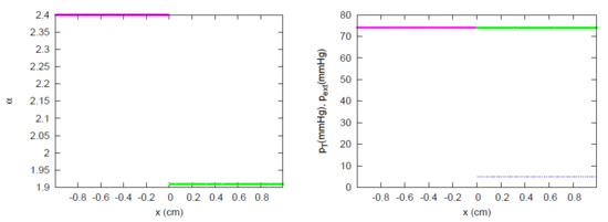
Figure 14. Section 3.1. JRP 2V0 in a two-vessel junction. Comparison between analytical (—) and numerical solutions at t = 0.002 s. The solution is equal to the initial one. Both vessels share the same value of $p_T$ at $x=0$.

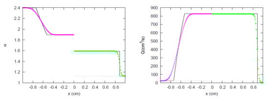
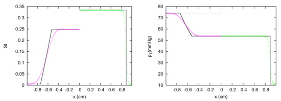
Figure 15. Section 3.1. JRP 2V1. Comparison between analytical (—) and numerical solutions at t = 0.002 s. The solution from vessel 1 to 2 is: a subsonic BDW, and a subsonic FCW, respectively. Both vessels share the same value of $p_T$ at $x=0$.

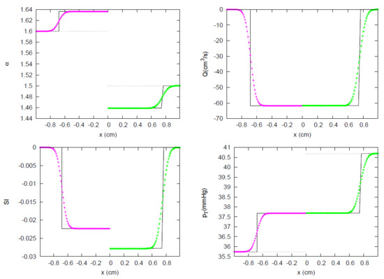
Figure 16. Section 3.1. JRP 2V2. Comparison between analytical (—) and numerical solutions at t = 0.002 s. The solution from vessel 1 to 2 is: a subsonic BCW, and a subsonic FDW, respectively. Both vessels share the same value of $p_T$ at $x=0$.

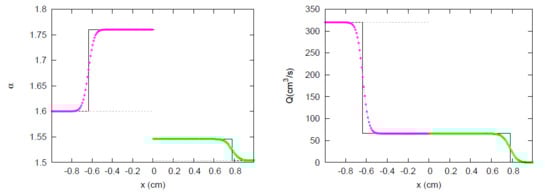
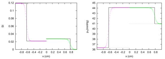
Figure 17. Section 3.1. JRP 2V3. Comparison between analytical (—) and numerical solutions at t = 0.002 s. The solution from vessel 1 to 2 is: a subsonic BCW, and a subsonic FCW, respectively. Both vessels share the same value of $p_T$ at $x=0$.

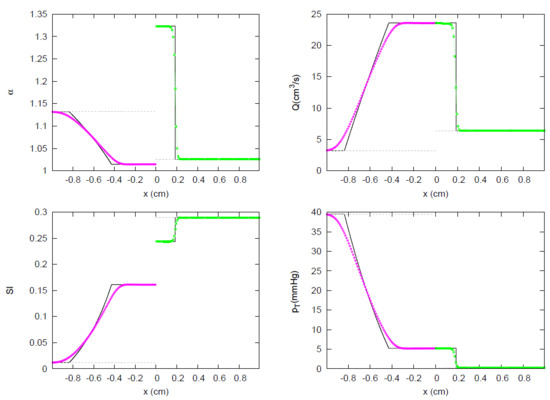
Figure 18. Section 3.1. JRP 2V4. Comparison between analytical (—) and numerical solutions at t = 0.001 s. The solution from vessel 1 to 2 is: a subsonic BDW, and a subsonic FCW, respectively. Both vessels share the same value of $p_T$ at $x=0$.

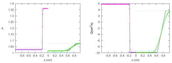
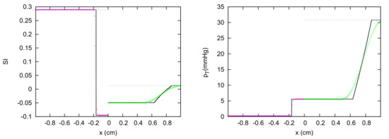
Figure 19. Section 3.1. JRP 2V5. Comparison between analytical (—) and numerical solutions at t = 0.001 s. The solution from vessel 1 to 2 is: a subsonic BCW, and a subsonic FDW, respectively. Both vessels share the same value of $p_T$ at $x=0$.

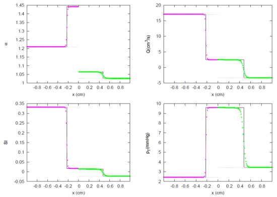
Figure 20. Section 3.1. JRP 2V6. Comparison between analytical (—) and numerical solutions at t = 0.001 s. The solution from vessel 1 to 2 is: a subsonic BCW, and a subsonic FCW, respectively. Both vessels share the same value of $p_T$ at $x=0$.

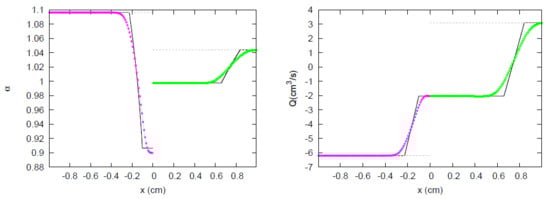
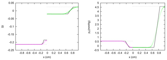
Figure 21. Section 3.1. JRP 2V7. Comparison between analytical (—) and numerical solutions at t = 0.002 s. The solution from vessel 1 to 2 is: a subsonic BDW, and a subsonic FDW, respectively. Both vessels share the same value of $p_T$ at $x=0$.

Test cases 2V8 and 2V9 involve supersonic flow. Figure 22, Figure 23 and Figure 24 show the exact solutions and the numerical solutions when the problems are defined as a RP in a single vessel with discontinuous properties. Being the flow supersonic, the exact solution of RP RpCase8 (Figure 22) is given by a contact wave at $x=0$ followed by a BDW (backward compression wave) and an FDW (forward decompression wave). In RP 2V9, the exact solution, plotted in Figure 24, is a contact wave at $x=0$ followed by an FCW (forward compression wave) and by an FDW (forward decompression wave). When solving both cases as a JRP using solver in (87), the analytical solution provided is different, since at most, one non-linear wave can be defined in each vessel of the confluence.

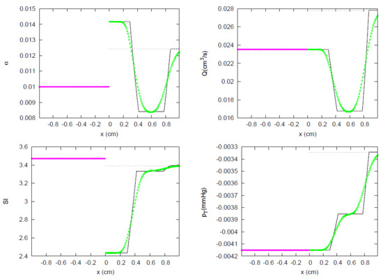
Figure 22. Section 3.1. RP 2V8 in a single vessel. Comparison between exact (—) and numerical solution using HLLS scheme at t = 0.3 s. The solution is a contact wave at $x=0$ followed by an FCW and an FDW.

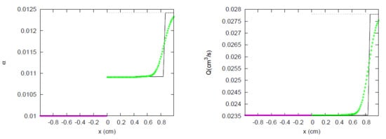
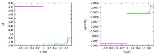
Figure 23. Section 3.1. JRP 2V8. Comparison between analytical (—) and numerical solutions at t = 0.3 s. The solution from vessel 1 to 2 is: a supersonic flow entering the confluence, and a supersonic FDW, respectively. Total pressure is not preserved at $x=0$.

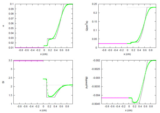
Figure 24. Section 3.1. RP 2V9 in a single vessel. Comparison between exact (—) and numerical solution using HLLS scheme at t = 0.2 s. The solution is a contact wave at $x=0$ followed by an FCW and an FDW.

The analytical solution provided by system in (87) for JRP 2V8 ensures no change of the solution at the left vessel of the junction, as observed for the exact solution, but in the right vessel only a supersonic FDW is defined (Figure 25). If we compare the analytical and the numerical solutions of the JRP, we observe supersonic flow conditions are kept in the left vessel, while in the right vessel, an FCW not defined in the analytical solution appears, followed by an FDW.

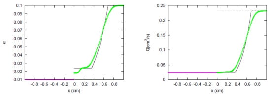
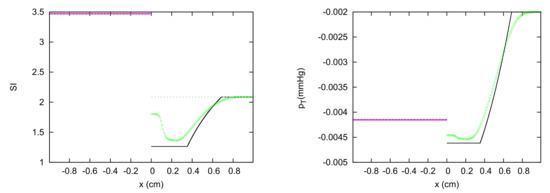
Figure 25. Section 3.1. JRP 2V9. Comparison between analytical (—) and numerical solutions at t = 0.2 s. The solution from vessel 1 to 2 is: a supersonic flow entering the confluence, and a supersonic FDW, respectively. Total pressure is not preserved at $x=0$.

For test 2V9, the analytical solution of the JRP ensures no change of the solution at the left vessel of the junction, as in the exact solution, but in the right vessel only a supersonic FDW is defined. The numerical solution for the JRP is a supersonic flow entering the confluence, followed by an FCW (not defined analytical solution) followed by an FDW. It can be observed that, for both exact solutions of the RPs 2V8 and 2V9 total energy, $p_T$, is preserved, while in JRPs 2V8 and 2V9, only mass conservation is preserved at the confluence in the analytical solution.

In test cases SubAtm1 to SubAtm3, the transition from subsonic flow conditions to sonic blockage conditions in a vessel is analyzed. To enforce this condition, pressure is atmospheric on the left side and sub-atmospheric on the right side of the RPs. Mechanical and geometrical properties and initial conditions are kept constant among experiments while the external pressure on the left side of the RP is decreased. The analytical solution of each JRP, equal to the exact solution of the RP, is plotted in Figure 26, Figure 27 and Figure 28 for test cases SubAtm1 to SubAtm3, respectively.

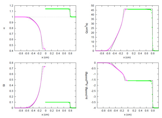
Figure 26. Section 3.1. JRP SubAtm1. Comparison between analytical (—) and numerical solutions at t = 0.005 s. The solution from vessel 1 to 2 is: a subsonic BDW, and a subsonic FCW, respectively. Both vessels share the same value of $p_T$ at $x=0$.

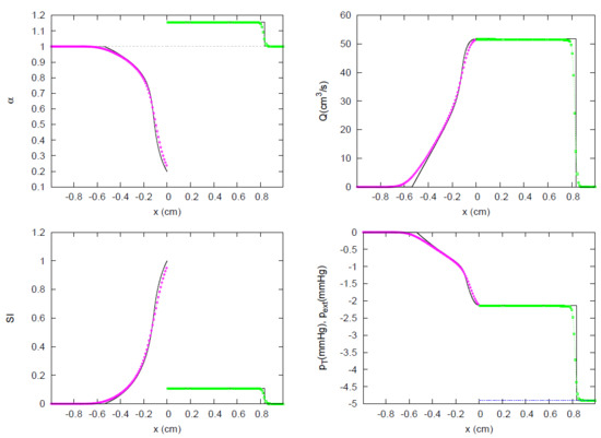
Figure 27. Section 3.1. JRP SubAtm2. Comparison between analytical (—) and numerical solutions at t = 0.005 s. The solution from vessel 1 to 2 is: a subsonic BDW including sonic limitation, and a subsonic FCW, respectively. Total pressure is not preserved at $x=0$.

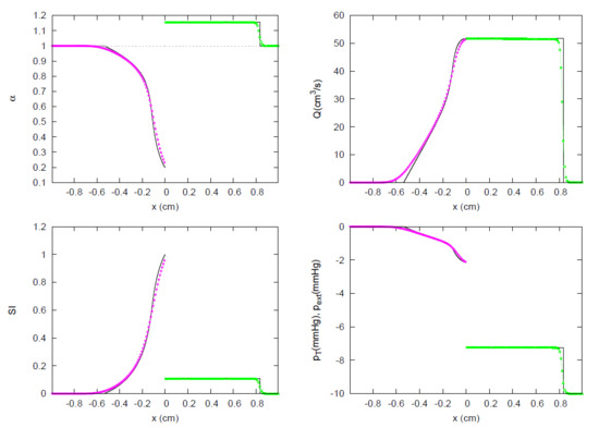
Figure 28. Section 3.1. JRP SubAtm3. Comparison between analytical (—) and numerical solutions at t = 0.005 s. The solution from vessel 1 to 2 is: a subsonic BDW including sonic limitation, and a subsonic FCW, respectively. Total pressure is not preserved at $x=0$.

The pressure variation in JRP SubAtm1 leads to a subsonic left moving rarefaction wave and a progressive narrowing of the vessel area. A contact discontinuity appears at $x=0$, leading to an abrupt expansion on the right side of the JRP, where sub-atmospheric pressure is imposed. In JRP SubAtm2 the suction on the left side of the JRP is increased and sonic conditions are forced across the contact discontinuity as shown in Figure 27. The moving rarefaction ends in the narrowest section now achieving sonic conditions. In both JRPs, SubAtm1 and SubAtm2, total energy is constant across the discontinuity. As sonic blockage has already been generated in JRP SubAtm2, the increase in the suction on the right side of the JRP in test case SubAtm3 does not change the analytical solution in the left vessel. On the other hand, Figure 26, Figure 27 and Figure 28, show how the numerical solutions of the JRP reproduce accurately the analytical solutions in all cases.

The performance of the proposed JRP solver in (87) is checked in situations of vessel collapse in test cases Collapse1 to Collapse4 in [28]. Figure 29 and Figure 30 show the exact solution of the RP Collapse1 in an artery. Supersonic initial flow conditions are imposed in all the vessel. In this RP, the solution remains constant over time on the left side of the RP. A stationary contact discontinuity is generated by the change in elasticity at $x=0$, where a constant value of total energy is observed and then, on the right side of the RP, a supersonic BDW develops leading to an extreme reduction of the vessel area. The vessel area is recovered along a supersonic FDW wave. When the vessel collapses between the BDW and the FDW, the value of the PWV increases exponentially against small variations in area. Although the HLLS solver is capable of generating a suitable solution for flow or velocity in the collapsed region, the numerical solution for the SI differs from the exact one since the value reached for the area is not as low as the value reached by the value of the solution exact.

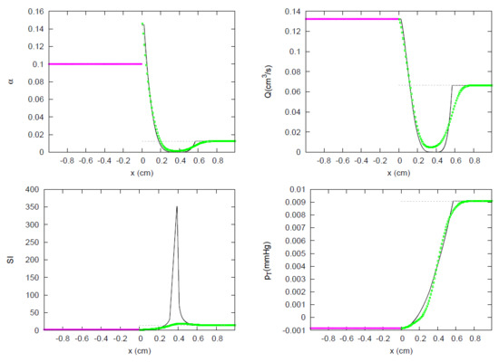
Figure 29. Section 3.1. RP Collapse1 in a single vessel. Comparison between exact (—) and numerical solution using HLLS scheme at t = 0.1 s. The solution is a stationary contact discontinuity at $x=0$ and a BDW followed by an FDW.

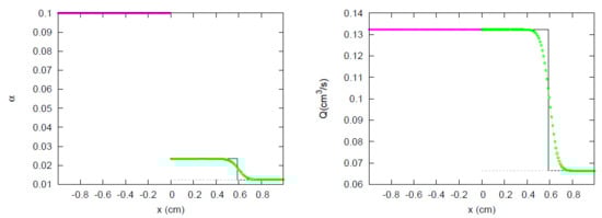
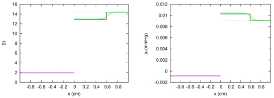
Figure 30. Section 3.1. JRP Collapse1. Comparison between analytical (—) and numerical solutions at t = 0.1 s. The solution from vessel 1 to 2 is: a supersonic flow entering the confluence, and a supersonic FCW, respectively. Total pressure is not preserved at $x=0$.

The solution changes when the JRP solver in (87) is applied to compute analytical solution for the test case Collapse1. The analytical solution does not change on the left side of the RP, but now, at the discontinuity, total energy does not remain constant. A supersonic FCW appears on the right side of the JRP, as only one wave can be defined at each branch of the confluence. The numerical solution to this JRP retains the exact solution in the left vessel, while in the right vessel, an FCW not defined in the analytical solution appears, followed by an FCW.

Test case Collapse2 has supersonic involves initial conditions on the left side and subsonic ones on the right. When solving this problem as a JRP, the analytical solution is equal to the exact solution of the equivalent RP in a single vessel, plotted in Figure 31. Numerical results can accurately reproduce the resulting supersonic BDW on the left and subsonic FDW on the right.

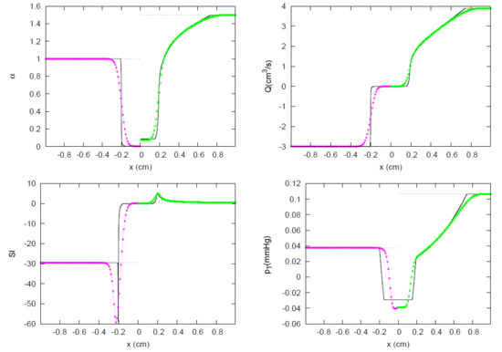
Figure 31. Section 3.1. JRP Collapse2. Comparison between analytical (—) and numerical solutions at t = 0.02 s. The solution from vessel 1 to 2 is: a supersonic BDW, and a subsonic FDW, respectively. Both vessels share the same value of $p_T$ at $x=0$.

JRP or equivalent RP Collapse3 is a vacuum problem where initial subsonic conditions lead to a supersonic BDW and a supersonic FDW, equal in both cases, as shown in Figure 32. When the solution of the JRM is computed numerically using the Godunov scheme, the results follow accurately the exact solution.

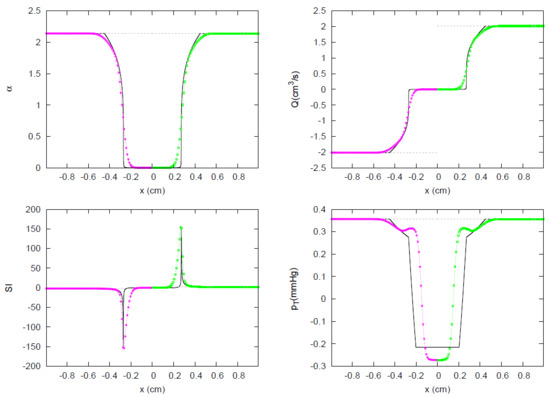
Figure 32. Section 3.1. JRP Collapse3. Comparison between analytical (—) and numerical solutions at t = 0.01 s. The solution from vessel 1 to 2 is: a supersonic BDW, and a supersonic FDW, respectively. Both vessels share the same value of $p_T$ at $x=0$.

When solving RP Collapse4, initially at rest, the exact solution, shown in Figure 33, leads to a supersonic BDW on the left side of the RP. This rarefaction crosses the interface $x=0$, ends on the right side and is followed by a supersonic FCW, as shown in Figure 33. When solving the problem as JRP the analytical solution leads to a subsonic BDW and a supersonic FCW on the left and right vessels respectively, as shown in Figure 34. Numerical solution of the JRP recovers accurately the analytical solution as shown in Figure 34.

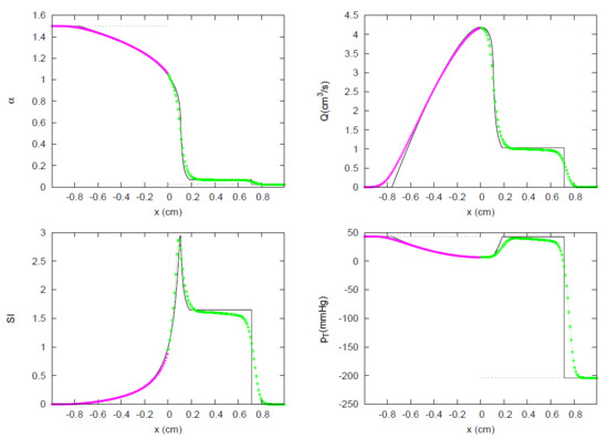
Figure 33. Section 3.1. RP Collapse4 in a single vessel Comparison between exact (—) and numerical solution using HLLS scheme at t = 0.001 s. The solution is a supersonic BDW followed by a supersonic FCW.

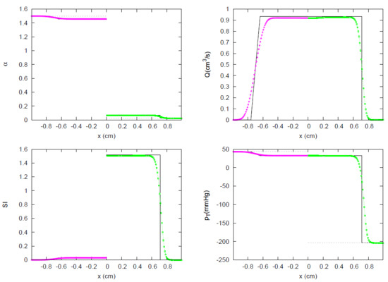
Figure 34. Section 3.1. JRP Collapse4. Comparison between analytical (—) and numerical solutions at t = 0.001 s. The solution from vessel 1 to 2 is: a subsonic BDW, and a supersonic FCW, respectively. Both vessels share the same value of $p_T$ at $x=0$.

3.2. JRP with Three Vessels

In this section, the analytical solution will be compared with the numerical solution for JRPs with three vessels. Initial conditions and mechanical and geometrical properties are presented in Table 2 for all the cases. Analytical solutions of the JRP in (87) are plotted in continuous line (—). Numerical solutions for vessels 1 to 3 are plotted using ($-\circ -$), ($-\square -$) and ($-△-$), respectively. External pressure $p_{ext}$ is plotted using ($---$).

Table 2. Three vessel confluence configuration. Test case, number of vessel k, father or daughter vessel $g_k$, reference diameter $d_{o,k}$ (mm), reference pulse wave velocity $c_{o,k}$ (cm ${\mathrm{s}}^{-1}$), reference pressure $p_{o,k}$ (mmHg), external pressure $p_{e,k}$, inital speed index $S{I}^n=u_k^n/c_k^n$, initial relative area ${\alpha }_k^n$ and transmural coefficients m and n.

Test Case	k	${\mathit{g}}_{\mathit{k}}$	${\mathit{d}}_{\mathit{o},\mathit{k}}$	${\mathit{c}}_{\mathit{o},\mathit{k}}$	${\mathit{p}}_{\mathit{o},\mathit{k}}$	${\mathit{p}}_{\mathit{e},\mathit{k}}$	${\mathit{S}\mathit{I}}^{\mathit{n}}$	${\mathit{\alpha }}^{\mathit{n}}$	m	n
3V1	1	1	27.000	119.27	0.0	0.0	0.00	0.500	10.0	−1.5
	2	−1	19.092	125.04	0.0	−10.0	0.00	1.000	10.0	−1.5
	3	−1	19.092	125.04	0.0	−10.0	0.00	1.000	10.0	−1.5
3V2	1	1	27.000	119.27	0.0	0.0	0.00	0.500	10.0	−1.5
	2	−1	19.092	125.04	0.0	−40.0	0.00	1.000	10.0	−1.5
	3	−1	19.092	125.04	0.0	−40.0	0.00	1.000	10.0	−1.5
3V3	1	1	27.000	119.27	0.0	0.0	0.00	0.500	10.0	−1.5
	2	−1	19.092	125.04	0.0	−100.0	0.00	1.000	10.0	−1.5
	3	−1	19.092	125.04	0.0	−100.0	0.00	1.000	10.0	−1.5
3V4	1	1	27.000	119.27	0.0	0.0	0.95	0.500	10.0	−1.5
	2	−1	19.092	125.04	0.0	−100.0	0.90	1.000	10.0	−1.5
	3	−1	19.092	125.04	0.0	−100.0	0.90	1.000	10.0	−1.5
3V5	1	1	27.000	119.27	0.0	0.0	1.00	0.500	10.0	−1.5
	2	−1	19.092	125.04	0.0	−10.0	0.00	1.000	10.0	−1.5
	3	−1	19.092	125.04	0.0	−10.0	0.00	1.000	10.0	−1.5
3V6	1	1	27.000	119.27	0.0	0.0	1.20	0.500	10.0	−1.5
	2	−1	19.092	125.04	0.0	−10.0	0.00	1.000	10.0	−1.5
	3	−1	19.092	125.04	0.0	−10.0	0.00	1.000	10.0	−1.5
3V7	1	1	27.000	119.27	0.0	0.0	0.60	1.000	10.0	−1.5
	2	−1	19.092	125.04	0.0	0.0	0.90	1.000	10.0	−1.5
	3	−1	19.092	125.04	0.0	0.0	0.90	1.000	10.0	−1.5
3V8	1	1	27.000	119.27	0.0	0.0	0.90	1.200	10.0	−1.5
	2	−1	19.092	125.04	0.0	0.0	1.10	1.000	10.0	−1.5
	3	−1	19.092	125.04	0.0	0.0	1.10	1.000	10.0	−1.5
3V9	1	1	27.000	119.27	0.0	0.0	0.00	1.200	10.0	−1.5
	2	−1	19.092	125.04	0.0	0.0	0.00	0.200	10.0	−1.5
	3	−1	19.092	125.04	0.0	0.0	0.00	0.200	10.0	−1.5
3V10	1	1	27.000	119.27	0.0	0.0	1.10	1.000	10.0	−1.5
	2	−1	19.092	125.04	0.0	0.0	1.10	1.000	10.0	−1.5
	3	−1	19.092	125.04	0.0	0.0	1.10	1.000	10.0	−1.5
3V11	1	1	27.000	119.27	0.0	0.0	−1.10	1.000	10.0	−1.5
	2	−1	19.092	125.04	0.0	0.0	−1.10	1.000	10.0	−1.5
	3	−1	19.092	125.04	0.0	0.0	−1.10	1.000	10.0	−1.5

JRPs 3V1 to 3V11 are RPs at junctions where three venous vessels are defined, one at the left side of the RP, and two at the right side. Initial conditions and mechanical and geometrical properties are equal at the right side of the RP. The analytical solution will be compared with the numerical solution for JRPs with three vessels.

In JRPs 3V1 to 3V3, vessel areas on the right side are larger than the vessel area on the left side. Initial conditions include zero velocity in all the domain. In absence of an external pressure, the variation in energy produced by the vessel deformation would generate a flow from the right vessels to the left vessel. However, in these cases the suction generated in the left side of the problem ensures a flow in the opposite direction, from the right vessel to the left vessels. Analytical solutions for the proposed JRP solver in (87) to test cases 3V1 to 3V3 are plotted in Figure 35, Figure 36 and Figure 37 respectively, and they show the evolution of the JRP when suction is increased in the right vessels. While in test case 3V1 a subsonic rarefaction is generated in the left vessel, in test case 3V2 conditions of sonic blockage have achieved. Further suction in JRP 3V3 is unable to generate a large value of flow and solutions for JRPs 3V2 and 3V3 are equal. Numerical solutions of the JRPs using the Godunov updating scheme in (15) reproduce the solution accurately for these three cases.

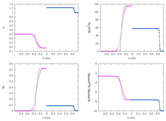
Figure 35. Section 3.2. Test 3V1. Comparison between analytical (—) and numerical solutions at t = 0.005 s. The solution from vessel 1 to 3 is: a subsonic BDW, a subsonic FCW, and a subsonic FCW, respectively. All vessels share the same value of $p_T$ at $x=0$.

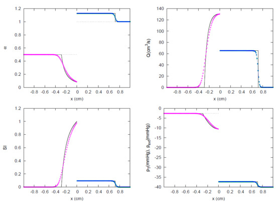
Figure 36. Section 3.2. Test 3V2. Comparison between analytical (—) and numerical solutions at t = 0.005 s. The solution from vessel 1 to 3 is: a subsonic BDW including sonic limitation, a subsonic FCW, and a subsonic FCW, respectively. Vessels 2, and 3 share the same value of $p_T$ at $x=0$.

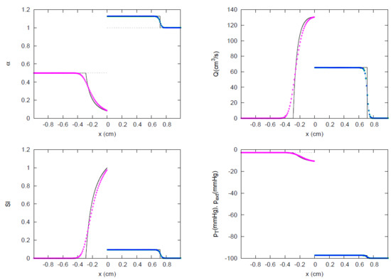
Figure 37. Section 3.2. Test 3V3. Comparison between analytical (—) and numerical solutions at t= 0.005 s. The solution from vessel 1 to 3 is: a subsonic BDW including sonic limitation, a subsonic FCW, and a subsonic FCW, respectively. Vessels 2, and 3 share the same value of $p_T$ at $x=0$.

In test case 3V4, the initial conditions for velocity in JRP 3V3 are modified and flow conditions close to the sonic regime are imposed in all vessels. The effect of the suction combined with the initial velocity generates again sonic blockage but now, in the right vessels, supersonic conditions are achieved along the FDW, as shown in Figure 38. Even the jump conditions in the FDW are subsonic, when the solution crosses by ${\alpha }_{PWV,min}$ the minimum value of PWV is defined, and a maximum value of $SI$ appears.

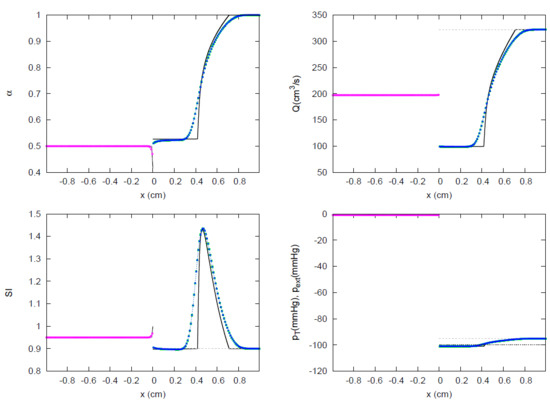
Figure 38. Section 3.2. Test 3V4. Comparison between analytical (—) and numerical solutions at t = 0.003 s. The solution from vessel 1 to 3 is: a subsonic BDW including sonic limitation, a subsonic FDW, and a subsonic FDW, respectively. Vessels 2, and 3 share the same value of $p_T$ at $x=0$.

In JRPs 3V5 and 3V6, test case 3V1 is modified and sonic conditions, $SI=1$, and super-sonic conditions, $SI=1.2$, are imposed, respectively. As shown in Figure 39 and Figure 40, in both cases the initial condition does not change over time in the left vessel, resulting in a supersonic outflow boundary condition at the junction, while an FCW appears in the right vessels.

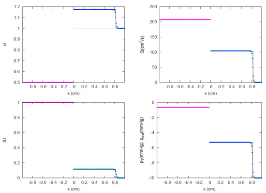
Figure 39. Section 3.2. Test 3V5. Comparison between analytical (—) and numerical solutions at t = 0.004 s. The solution from vessel 1 to 3 is: a supersonic flow entering the confluence, a subsonic FCW, and a subsonic FCW, respectively. Vessels 2, and 3 share the same value of $p_T$ at $x=0$.

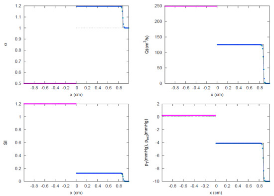
Figure 40. Section 3.2. Test 3V6. Comparison between analytical (—) and numerical solutions at t = 0.004 s. The solution from vessel 1 to 3 is: a supersonic flow entering the confluence, a subsonic FCW, and a subsonic FCW, respectively. Vessels 2, and 3 share the same value of $p_T$ at $x=0$.

In test case 3V7 the vessel area is equal to the reference vessel area in all vessels, $\alpha =1$, and subsonic flow conditions are imposed in all vessels (Figure 41). The resulting solution produces a subsonic-supersonic transition at the junction with the same value of total energy for the right vessels, with a subsonic BDW in the left vessel and a supersonic FDW in the right vessels. Numerical solutions do not converge to this solution, leading to a two-wave pattern in the right side vessels.

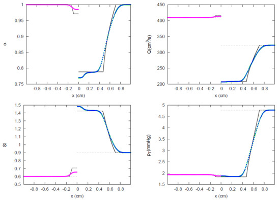
Figure 41. Section 3.2. Test 3V7. Comparison between analytical (—) and numerical solutions at t = 0.003 s. The solution from vessel 1 to 3 is: a subsonic BDW, a subsonic FDW, and a subsonic FDW, respectively. All vessels share the same value of $p_T$ at $x=0$.

Subsonic and supersonic initial conditions in the left and right side of the JRP in test case 3V8 generate a subsonic BDW including sonic limitation and subsonic FCW. As plotted in Figure 42, the numerical solution generates a different level of energy in the vicinity of the junction if compared with the analytical solution. Therefore, it does not converge to the analytical solution and generates a BCW in the left vessel and an identical FCW for the right vessels.

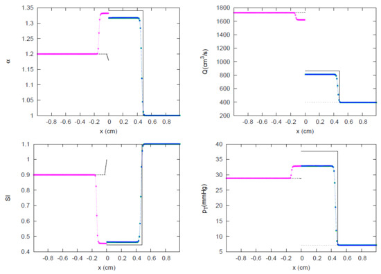
Figure 42. Section 3.2. Test 3V8. Comparison between analytical (—) and numerical solutions at t = 0.001 s. The solution from vessel 1 to 3 is: a subsonic BDW including sonic limitation, a subsonic FCW, and a subsonic FCW, respectively. Vessels 2, and 3 share the same value of $p_T$ at $x=0$.

A large pressure gradient is forced in test case 3V9 by imposing a large variation in the vessel deformation between the left vessel and the right vessels. The analytical solution in Figure 43 is a subsonic BDW in the left vessel, and a supersonic FCW in the right vessels, which share the same level of energy at the junction.

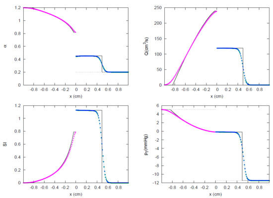
Figure 43. Section 3.2. Test 3V9. Comparison between analytical (—) and numerical solutions at t = 0.003 s. The solution from vessel 1 to 3 is: a subsonic BDW, a supersonic FCW, and a supersonic FCW, respectively. All vessels share the same value of $p_T$ at $x=0$.

Initial supersonic conditions are imposed in all vessels in test case 3V10, as plotted in Figure 44. The analytical solution is a supersonic flow entering the confluence from the left vessel, and a supersonic FDW in the outlet vessels. Supersonic left vessel conditions remain unaltered over time and therefore left vessel only takes part in the mass conservation equation at the junction. Right vessels, experience the supersonic conditions at the junctions too, and share the same level of energy. The numerical solution reproduces the main features of the solution, although a small perturbation is visible at the vicinity of the junction. In test case 3V11, the flow moves in the opposite direction, from right to left, and again all vessels have initial supersonic conditions. Now initial conditions remain unaltered over time in the right vessels, and they only take part in mass conservation, whereas a supersonic BCW appears in the right vessel (Figure 45).

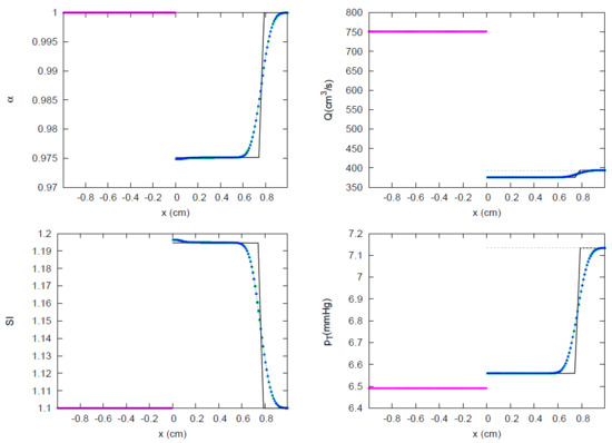
Figure 44. Section 3.2. Test 3V10. Comparison between analytical (—) and numerical solutions at t = 0.003 s. The solution from vessel 1 to 3 is: a supersonic flow entering the confluence, a supersonic FDW, and a supersonic FDW, respectively. Vessels 2, and 3 share the same value of $p_T$ at $x=0$.

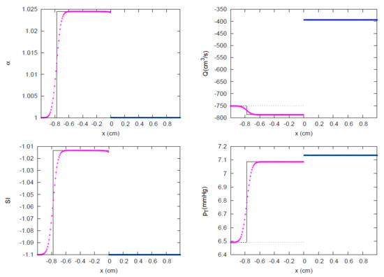
Figure 45. Section 3.2. Test 3V11. Comparison between analytical (—) and numerical solutions at t = 0.003 s. The solution from vessel 1 to 3 is: a supersonic BCW, a supersonic flow entering the confluence, and a supersonic flow entering the confluence, respectively. Total pressure is not preserved at $x=0$.

3.3. JRP with Four Vessels

In the following test cases the analytical solution and the numerical solutions for RPs at junctions with four vessels are presented. In all test cases, the four vessels have the same mechanical and geometrical properties, listed in Table 3, Table 4 and Table 5, with two vessels on the left and the other two on the right of the junction. Analytical solutions of the JRP in (87) are plotted in continuous line (—). Numerical solutions for vessels 1 to 4 are plotted using ($-\circ -$), ($-\square -$), ($-△-$) and ($-▽-$), respectively. External pressure $p_{ext}$ is plotted using ($---$).

Table 3. Confluence configuration with four vessels. Test case, number of vessel k, father or daughter vessel $g_k$, reference diameter $d_{o,k}$ (mm), reference pulse wave velocity $c_{o,k}$ (cm ${\mathrm{s}}^{-1}$), reference pressure $p_{o,k}$ (mmHg), external pressure $p_{e,k}$, initial speed index $S{I}^n=u_k^n/c_k^n$, initial relative area ${\alpha }_k^n$ and transmural coefficients m and n.

Test Case	k	${\mathit{g}}_{\mathit{k}}$	${\mathit{d}}_{\mathit{o},\mathit{k}}$	${\mathit{c}}_{\mathit{o},\mathit{k}}$	${\mathit{p}}_{\mathit{o},\mathit{k}}$	${\mathit{p}}_{\mathit{e},\mathit{k}}$	${\mathit{S}\mathit{I}}^{\mathit{n}}$	${\mathit{\alpha }}^{\mathit{n}}$	m	n
4V1	1	1	30.500	511.00	0.0	0.0	0.00	1.200	10.0	−1.5
	2	1	30.500	511.00	0.0	0.0	0.00	1.100	10.0	−1.5
	3	−1	30.500	511.00	0.0	−40.0	0.00	0.900	10.0	−1.5
	4	−1	30.500	511.00	0.0	−80.0	0.00	0.800	10.0	−1.5
4V2	1	1	30.500	511.00	0.0	−40.0	0.00	0.900	10.0	−1.5
	2	1	30.500	511.00	0.0	−80.0	0.00	0.800	10.0	−1.5
	3	−1	30.500	511.00	0.0	0.0	0.00	1.200	10.0	−1.5
	4	−1	30.500	511.00	0.0	0.0	0.00	1.100	10.0	−1.5
4V3	1	1	30.500	118.72	0.0	−40.0	0.00	0.900	10.0	−1.5
	2	1	30.500	118.72	0.0	−40.0	0.00	0.800	10.0	−1.5
	3	−1	30.500	118.72	0.0	0.0	0.00	1.200	10.0	−1.5
	4	−1	30.500	118.72	0.0	0.0	0.00	1.100	10.0	−1.5
4V4	1	1	30.500	118.72	0.0	−40.0	0.00	0.900	10.0	−1.5
	2	1	30.500	118.72	0.0	−80.0	0.00	0.800	10.0	−1.5
	3	−1	30.500	118.72	0.0	0.0	0.00	1.200	10.0	−1.5
	4	−1	30.500	118.72	0.0	0.0	0.00	1.100	10.0	−1.5
4V5	1	1	30.500	118.72	0.0	0.0	0.00	1.200	10.0	−1.5
	2	1	30.500	118.72	0.0	0.0	0.00	1.100	10.0	−1.5
	3	−1	30.500	118.72	0.0	0.0	0.00	0.200	10.0	−1.5
	4	−1	30.500	118.72	0.0	0.0	0.00	0.300	10.0	−1.5
4V6	1	1	30.500	118.72	0.0	0.0	0.00	0.200	10.0	−1.5
	2	1	30.500	118.72	0.0	0.0	0.00	0.300	10.0	−1.5
	3	−1	30.500	118.72	0.0	0.0	0.00	1.200	10.0	−1.5
	4	−1	30.500	118.72	0.0	0.0	0.00	1.100	10.0	−1.5
4V7	1	1	30.500	118.72	0.0	0.0	0.00	0.100	10.0	−1.5
	2	1	30.500	118.72	0.0	0.0	0.00	0.300	10.0	−1.5
	3	−1	30.500	118.72	0.0	0.0	0.00	1.200	10.0	−1.5
	4	−1	30.500	118.72	0.0	0.0	0.00	1.100	10.0	−1.5
4V8	1	1	30.500	118.72	0.0	0.0	−1.10	0.100	10.0	−1.5
	2	1	30.500	118.72	0.0	0.0	−0.90	0.300	10.0	−1.5
	3	−1	30.500	118.72	0.0	0.0	0.00	1.200	10.0	−1.5
	4	−1	30.500	118.72	0.0	0.0	0.00	1.100	10.0	−1.5
4V9	1	1	30.500	118.72	0.0	0.0	0.00	1.200	10.0	−1.5
	2	1	30.500	118.72	0.0	0.0	0.00	1.100	10.0	−1.5
	3	−1	30.500	118.72	0.0	0.0	1.10	0.100	10.0	−1.5
	4	−1	30.500	118.72	0.0	0.0	0.90	0.300	10.0	−1.5
4V10	1	1	30.500	118.72	0.0	0.0	1.10	0.100	10.0	−1.5
	2	1	30.500	118.72	0.0	0.0	0.90	0.300	10.0	−1.5
	3	−1	30.500	118.72	0.0	0.0	0.00	1.200	10.0	−1.5
	4	−1	30.500	118.72	0.0	0.0	0.00	1.100	10.0	−1.5

Table 4. Confluence configuration with four vessels. Test case, number of vessel k, father or daughter vessel $g_k$, reference diameter $d_{o,k}$ (mm), reference pulse wave velocity $c_{o,k}$ (cm ${\mathrm{s}}^{-1}$), reference pressure $p_{o,k}$ (mmHg), external pressure $p_{e,k}$, initial speed index $S{I}^n=u_k^n/c_k^n$, initial relative area ${\alpha }_k^n$ and transmural coefficients m and n.

Test Case	k	${\mathit{g}}_{\mathit{k}}$	${\mathit{d}}_{\mathit{o},\mathit{k}}$	${\mathit{c}}_{\mathit{o},\mathit{k}}$	${\mathit{p}}_{\mathit{o},\mathit{k}}$	${\mathit{p}}_{\mathit{e},\mathit{k}}$	${\mathit{S}\mathit{I}}^{\mathit{n}}$	${\mathit{\alpha }}^{\mathit{n}}$	m	n
4V11	1	1	30.500	118.72	0.0	0.0	0.00	1.200	10.0	−1.5
	2	1	30.500	118.72	0.0	0.0	0.00	1.100	10.0	−1.5
	3	−1	30.500	118.72	0.0	0.0	−1.10	0.100	10.0	−1.5
	4	−1	30.500	118.72	0.0	0.0	−0.90	0.300	10.0	−1.5
4V12	1	1	30.500	118.72	0.0	0.0	−1.10	1.200	10.0	−1.5
	2	1	30.500	118.72	0.0	0.0	−1.20	1.100	10.0	−1.5
	3	−1	30.500	118.72	0.0	0.0	−1.10	0.100	10.0	−1.5
	4	−1	30.500	118.72	0.0	0.0	−1.20	0.300	10.0	−1.5
4V13	1	1	30.500	118.72	0.0	0.0	1.10	0.100	10.0	−1.5
	2	1	30.500	118.72	0.0	0.0	1.20	0.300	10.0	−1.5
	3	−1	30.500	118.72	0.0	0.0	1.10	1.200	10.0	−1.5
	4	−1	30.500	118.72	0.0	0.0	1.20	1.100	10.0	−1.5
4V14	1	1	30.500	118.72	0.0	0.0	−1.10	1.200	10.0	−1.5
	2	1	30.500	118.72	0.0	0.0	−0.90	1.100	10.0	−1.5
	3	−1	30.500	118.72	0.0	0.0	−1.10	0.100	10.0	−1.5
	4	−1	30.500	118.72	0.0	0.0	−1.20	0.300	10.0	−1.5
4V15	1	1	30.500	118.72	0.0	0.0	−1.10	1.200	10.0	−1.5
	2	1	30.500	118.72	0.0	0.0	−1.20	1.100	10.0	−1.5
	3	−1	30.500	118.72	0.0	0.0	−0.90	0.100	10.0	−1.5
	4	−1	30.500	118.72	0.0	0.0	−1.20	0.300	10.0	−1.5
4V16	1	1	30.500	118.72	0.0	0.0	1.10	1.100	10.0	−1.5
	2	1	30.500	118.72	0.0	0.0	1.20	1.300	10.0	−1.5
	3	−1	30.500	118.72	0.0	0.0	1.10	0.600	10.0	−1.5
	4	−1	30.500	118.72	0.0	0.0	0.90	0.500	10.0	−1.5
4V17	1	1	30.500	118.72	0.0	0.0	0.90	0.100	10.0	−1.5
	2	1	30.500	118.72	0.0	0.0	1.20	0.300	10.0	−1.5
	3	−1	30.500	118.72	0.0	0.0	1.10	0.600	10.0	−1.5
	4	−1	30.500	118.72	0.0	0.0	1.20	0.200	10.0	−1.5
4V18	1	1	30.500	118.72	0.0	0.0	0.90	0.100	10.0	−1.5
	2	1	30.500	118.72	0.0	0.0	1.20	0.300	10.0	−1.5
	3	−1	30.500	118.72	0.0	0.0	1.10	0.600	10.0	−1.5
	4	−1	30.500	118.72	0.0	0.0	0.90	0.200	10.0	−1.5
4V19	1	1	30.500	118.72	0.0	0.0	−0.90	0.100	10.0	−1.5
	2	1	30.500	118.72	0.0	0.0	−1.20	0.300	10.0	−1.5
	3	−1	30.500	118.72	0.0	0.0	−1.10	0.600	10.0	−1.5
	4	−1	30.500	118.72	0.0	0.0	−0.90	0.200	10.0	−1.5
4V20	1	1	30.500	118.72	0.0	0.0	−0.90	0.100	10.0	−1.5
	2	1	30.500	118.72	0.0	0.0	1.20	0.300	10.0	−1.5
	3	−1	30.500	118.72	0.0	0.0	1.10	0.600	10.0	−1.5
	4	−1	30.500	118.72	0.0	0.0	−0.90	0.200	10.0	−1.5

Table 5. Confluence configuration with four vessels. Test case, number of vessel k, father or daughter vessel $g_k$, reference diameter $d_{o,k}$ (mm), reference pulse wave velocity $c_{o,k}$ (cm ${\mathrm{s}}^{-1}$), reference pressure $p_{o,k}$ (mmHg), external pressure $p_{e,k}$, initial speed index $S{I}^n=u_k^n/c_k^n$, initial relative area ${\alpha }_k^n$ and transmural coefficients m and n.

Test Case	k	${\mathit{g}}_{\mathit{k}}$	${\mathit{d}}_{\mathit{o},\mathit{k}}$	${\mathit{c}}_{\mathit{o},\mathit{k}}$	${\mathit{p}}_{\mathit{o},\mathit{k}}$	${\mathit{p}}_{\mathit{e},\mathit{k}}$	${\mathit{S}\mathit{I}}^{\mathit{n}}$	${\mathit{\alpha }}^{\mathit{n}}$	m	n
4V21	1	1	30.500	118.72	0.0	0.0	−1.10	0.600	10.0	−1.5
	2	1	30.500	118.72	0.0	0.0	0.90	0.200	10.0	−1.5
	3	−1	30.500	118.72	0.0	0.0	0.90	0.100	10.0	−1.5
	4	−1	30.500	118.72	0.0	0.0	−1.20	0.300	10.0	−1.5
4V22	1	1	30.500	118.72	0.0	0.0	1.10	0.100	10.0	−1.5
	2	1	30.500	118.72	0.0	0.0	−1.20	0.300	10.0	−1.5
	3	−1	30.500	118.72	0.0	0.0	1.10	1.200	10.0	−1.5
	4	−1	30.500	118.72	0.0	0.0	−1.20	1.100	10.0	−1.5
4V23	1	1	30.500	118.72	0.0	0.0	1.10	0.100	10.0	−1.5
	2	1	30.500	118.72	0.0	0.0	0.00	0.300	10.0	−1.5
	3	−1	30.500	118.72	0.0	−30.0	1.10	1.200	10.0	−1.5
	4	−1	30.500	118.72	0.0	−40.0	1.20	1.100	10.0	−1.5
4V24	1	1	30.500	118.72	0.0	0.0	1.10	0.100	10.0	−1.5
	2	1	30.500	118.72	0.0	0.0	0.00	0.300	10.0	−1.5
	3	−1	30.500	118.72	0.0	−30.0	1.10	0.100	10.0	−1.5
	4	−1	30.500	118.72	0.0	−40.0	1.20	0.200	10.0	−1.5
4V25	1	1	30.500	118.72	0.0	0.0	0.90	0.100	10.0	−1.5
	2	1	30.500	118.72	0.0	0.0	1.10	0.300	10.0	−1.5
	3	−1	30.500	118.72	0.0	−30.0	−1.20	0.100	10.0	−1.5
	4	−1	30.500	118.72	0.0	−40.0	−0.90	0.200	10.0	−1.5
4V26	1	1	30.500	118.72	0.0	0.0	1.10	0.100	10.0	−1.5
	2	1	30.500	118.72	0.0	30.0	0.90	0.300	10.0	−1.5
	3	−1	30.500	118.72	0.0	0.0	−0.80	0.100	10.0	−1.5
	4	−1	30.500	118.72	0.0	−40.0	−1.20	0.200	10.0	−1.5
4V27	1	1	30.500	118.72	0.0	0.0	−1.10	0.100	10.0	−1.5
	2	1	30.500	118.72	0.0	0.0	−0.90	0.300	10.0	−1.5
	3	−1	30.500	118.72	0.0	0.0	0.80	0.100	10.0	−1.5
	4	−1	30.500	118.72	0.0	0.0	1.20	0.200	10.0	−1.5

In this JRP, 4V1, all vessels are initially at rest, each one with a different level of deformation, $\alpha$ (Figure 46). While in left vessels 1 and 2 the deformation parameter $\alpha >1$, in right vessels 3 and 4 we impose $\alpha <1$. The pressure discontinuity distribution is enlarged by the suction in right vessels 3 and 4 and generates a sonic BDW and a subsonic BDW for vessels 1 and 2, and subsonic FCWs for vessels 3 and 4. In vessel 1, sonic limitation is observed at the junction. Vessel 1 also exhibits the greatest level of energy at the junction, while vessels 2 to 4, provide the same level of energy at the confluence.

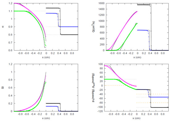
Figure 46. Section 3.3. Test 4V1. Comparison between analytical (—) and numerical solutions at t = 0.0007 s. The solution of test case 4V1 from vessels 1 to 4 is: a subsonic BDW including sonic limitation, a subsonic BDW, a subsonic FCW, and a subsonic FCW, respectively. Vessels 2, 3, and 4 share the same value of $p_T$ at $x=0$.

In test case 4V2, the initial conditions are switched to generate the same exact wave pattern, but in the opposite direction, $u\le 0$, involving again sonic flow limitation in one vessel (Figure 47). The JRP solver presented in this work converges to the expected physically based solution.

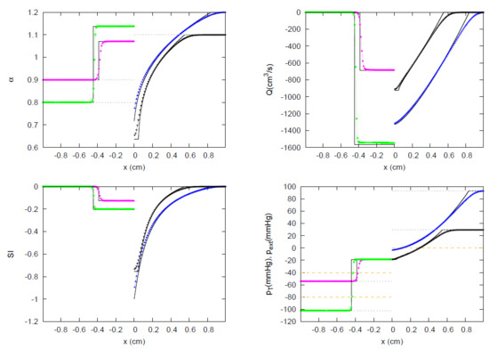
Figure 47. Section 3.3. Test 4V2. Comparison between analytical (—) and numerical solutions at t = 0.0007 s. The solution of test case 4V2 from vessels 1 to 4 is: a subsonic BCW, a subsonic BCW, a subsonic FDW including sonic limitation, and a subsonic FDW, respectively. Vessels 1, 2, and 4 share the same value of $p_T$ at $x=0$.

In JRP 4V3 (Figure 48), the mechanical properties in 4V2 are changed by decreasing the PWV in all vessels. The same level of suction is prescribed for vessels 1 and 2. Now, the vessels are more easily deformable and, despite the level of suction has been reduced if compared with test case 4V2, sonic blockage appears in vessels 3 and 4 at the junction. Only vessels 1 and 2 share the same level of energy at the junction, where a subsonic BCW appears in each branch.

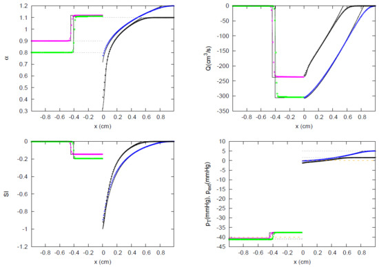
Figure 48. Section 3.3. Test 4V3. Comparison between analytical (—) and numerical solutions at t = 0.003 s. The solution of test case 4V3 from vessels 1 to 4 is: a subsonic BCW, a subsonic BCW, a subsonic FDW including sonic limitation, and a subsonic FDW including sonic limitation, respectively. Vessels 1, and 2 share the same value of $p_T$ at $x=0$.

In test case 4V4 (Figure 49), the suction in vessel 2 is increased. Now vessels 1, 3 and 4 contribute to the flow mass towards vessel 2 (Figure 49). As sonic blockage for vessels 1, 3 and 4 is produced, they exhibit different values of total energy at the junction. The solution for vessel 2 is a subsonic BCW.

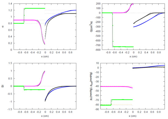
Figure 49. Section 3.3. Test 4V4. Comparison between analytical (—) and numerical solutions at t = 0.003 s. The solution of test case 4V4 from vessels 1 to 4 is: a subsonic BDW including sonic limitation, a subsonic BCW, a subsonic FDW including sonic limitation, and a subsonic FDW including sonic limitation, respectively. Total pressure is not preserved at $x=0$.

In test case 4V5 (Figure 50), the large jump in the deformation parameter, $\alpha =1.2$ at the left and $\alpha =0.2$ at the right, generates a BDW for vessels 1 (ending in sonic limitation) and 2, and a supersonic FCW and a subsonic FCW for vessels 3 and 4, respectively. Subsonic vessels 2 and 4 retain the same value of energy at the junction shared by the supersonic FCW in inflow vessel 3.

Figure 50. Section 3.3. Test 4V5. Comparison between analytical (—) and numerical solutions at t = 0.003 s. The solution of test case 4V5 from vessels 1 to 4 is: a subsonic BDW including sonic limitation, a subsonic BDW, a supersonic FCW, and a subsonic FCW, respectively. Vessels 2, 3, and 4 share the same value of $p_T$ at $x=0$.

When the jump in pressure in test case 4V5 is inverted, the solution, in test case 4V6 (Figure 51) is exactly equal, but in the opposite direction, $u\le 0$.

Figure 51. Section 3.3. Test 4V6. Comparison between analytical (—) and numerical solutions at t = 0.003 s. The solution of test case 4V6 from vessels 1 to 4 is: a supersonic BCW, a subsonic BCW, a subsonic FDW including sonic limitation, and a subsonic FDW, respectively. Vessels 1, 2, and 4 share the same value of $p_T$ at $x=0$.

Test case 4V7 (Figure 52) is defined by reducing the minimum value of the deformation parameter to $\alpha =0.1$ in test case 4V6. The solution for vessels 3 and 4, on the right side of the junction, remains unaltered. The flow distribution changes on the right side generating a supersonic and a subsonic BCW for vessels 1 and 2, respectively. Except in vessel 3, where sonic limitation is produced, all vessels share the same value of energy being subsonic or supersonic.

Figure 52. Section 3.3. Test 4V7. Comparison between analytical (—) and numerical solutions at t = 0.003 s. The solution of test case 4V7 from vessels 1 to 4 is: a supersonic BCW, a subsonic BCW, a subsonic FDW including sonic limitation, and a subsonic FDW, respectively. Vessels 1, 2, and 4 share the same value of $p_T$ at $x=0$.

In test case 4V8 (Figure 53), supersonic and subsonic conditions for inflow vessels 1 and 2 are prescribed. Rest conditions are imposed the right side of the JRP. The solution generates a subsonic FDW for vessel 4 and supersonic BDW for vessels 1 and 2, all of them connected by the same level of energy at the junction. Vessel 3, experiencing sonic blockage, participates in mass conservation but not in the energy state at the junction.

Figure 53. Section 3.3. Test 4V8. Comparison between analytical (—) and numerical solutions at t = 0.001 s. The solution of test case 4V8 from vessels 1 to 4 is: a supersonic BCW, a supersonic BCW, a subsonic FDW including sonic limitation, and a subsonic FDW, respectively. Vessels 1, 2, and 4 share the same value of $p_T$ at $x=0$.

In test case 4V9 (Figure 54), the initial conditions are modified to generate the same solution as the one generated in test case 4V9, with $u>0$.

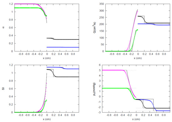
Figure 54. Section 3.3. Test 4V9. Comparison between analytical (—) and numerical solutions at t = 0.001 s. The solution of test case 4V9 from vessels 1 to 4 is: a subsonic BDW including sonic limitation, a subsonic BDW, a supersonic FCW, and a supersonic FCW, respectively. Vessels 2, 3, and 4 share the same value of $p_T$ at $x=0$.

In test case 4V10 (Figure 55), maximum deformation values are found at the right side of the JRP together with zero velocity. Minimum deformation values involving sonic and supersonic conditions are found at the left side of the JRP. Right vessels 3 and 4 develop a BDW, while vessels 1 and 2 experience the generation of subsonic BCW. The solution at $x=0$ is subsonic for all branches, exhibiting the value of energy at the junction.

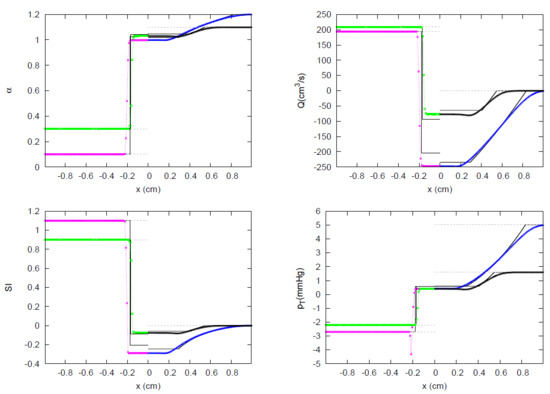
Figure 55. Section 3.3. Test 4V10. Comparison between analytical (—) and numerical solutions at t = 0.003 s. The solution of test case 4V10 from vessels 1 to 4 is: a subsonic BCW, a subsonic BCW, a subsonic FDW, and a subsonic FDW, respectively. All vessels share the same value of $p_T$ at $x=0$.

Maximum deformation values together with rest conditions are prescribed at the left side of the JRP in test case 4V11 (Figure 56). Supersonic and subsonic conditions with $u<0$ are imposed on the right side. The jump in pressure generates a positive flow, restrained by the initial flow conditions in the right vessels. In right vessels 3 and 4 a subsonic FCW is developed, while in vessels 1 and 2 a subsonic BDW is generated. The solution at $x=0$ is subsonic for all vessels.

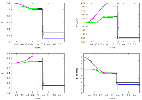
Figure 56. Section 3.3. Test 4V11. Comparison between analytical (—) and numerical solutions at t = 0.003 s. The solution of test case 4V11 from vessels 1 to 4 is: a subsonic BDW, a subsonic BDW, a subsonic FCW, and a subsonic FCW, respectively. All vessels share the same value of $p_T$ at $x=0$.

Supersonic initial conditions are initially imposed on all vessels in test case 4V12 (Figure 57) with $u<0$, retaining maximum deformation values at the left and minimum deformation values at the right. The solution generates supersonic BDWs for vessels 1 and 2. Initial conditions in vessels 3 and 4 do not change over time. Even the flow is supersonic at $x=0$ for vessels 1 and 2; they share the same level of $p_T$ at this point.

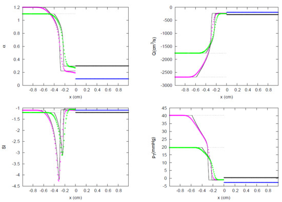
Figure 57. Section 3.3. Test 4V12. Comparison between analytical (—) and numerical solutions at t = 0.001 s. The solution of test case 4V12 from vessel s1 to 4 is: a supersonic BDW, a supersonic BDW, a supersonic flow entering the confluence, and a supersonic flow entering the confluence, respectively. Vessels 1 and 2 share the same value of $p_T$ at $x=0$.

In test case 4V13 (Figure 58), supersonic initial conditions are initially imposed to define the same wave pattern as in test case 4V12, but in the opposite direction.

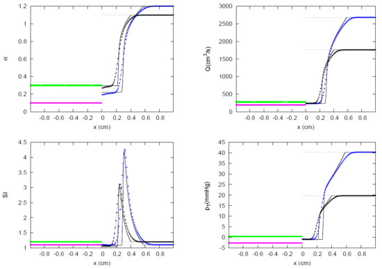
Figure 58. Section 3.3. Test 4V13. Comparison between analytical (—) and numerical solutions at t = 0.001 s. The solution of test case 4V13 from vessels 1 to 4 is: a supersonic flow entering the confluence, a supersonic flow entering the confluence, a supersonic FDW, and a supersonic FDW, respectively. Vessels 3 and 4 share the same value of $p_T$ at $x=0$.

Supersonic initial conditions are imposed in outflow vessels 3 and 4 in test case 4V14 (Figure 59), where now the minimum vessel area has been defined, retaining their initial state over time, and therefore only contributing to the mass balance at the junction. Vessels 1 and 2 develop supersonic BDWs. They share the same level of energy at the junction despite ending at $x=0$ in supersonic and subsonic conditions, respectively.

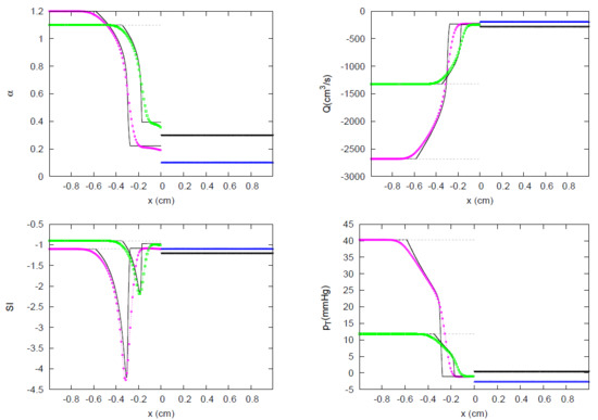
Figure 59. Section 3.3. Test 4V14. Comparison between analytical (—) and numerical solutions at t = 0.001 s. The solution of test case 4V14 from vessels 1 to 4 is: a supersonic BDW, a subsonic BDW, a supersonic flow entering the confluence, and a supersonic flow entering the confluence, respectively. Vessels 1 and 2 share the same value of $p_T$ at $x=0$.

Subsonic initial conditions for vessel 3 and supersonic initial conditions for vessels 1, 2 and 4 are imposed in test case 4V15 (Figure 60). Vessels 1, 2, and 3 share the same value of $p_T$ at $x=0$, and an FCW and two BDWs are generated for vessels 1, 2, and 3 respectively. Flow in vessel 4 does not change over time.

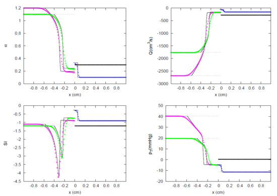
Figure 60. Section 3.3. Test 4V15. Comparison between analytical (—) and numerical solutions at t = 0.001 s. The solution of test case 4V15 from vessels 1 to 4 is: a supersonic BDW, a supersonic BDW, a subsonic FCW, and a supersonic flow entering the confluence, respectively. Vessels 1, 2, and 3 share the same value of $p_T$ at $x=0$.

In 4V16 (Figure 61) supersonic initial conditions are initially imposed in vessels 1 and 2. While for vessel 2 the solution remains invariant over time, it can be seen how for vessel 1, a BCW is developed, allowing transmission of the information downstream the junction. Vessels 1, 3 and 4 shares the same level of energy at $x=0$. In vessels 3 and 4, a subsonic FCW is observed.

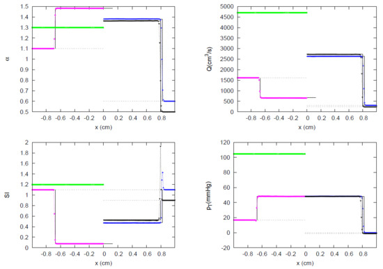
Figure 61. Section 3.3. Test 4V16. Comparison between analytical (—) and numerical solutions at t = 0.002 s. The solution of test case 4V16 from vessels 1 to 4 is: a subsonic BCW, a supersonic flow entering the confluence, a subsonic FCW, and a subsonic FCW, respectively. Vessels 1, 3, and 4 share the same value of $p_T$ at $x=0$.

Collapsed and partially collapsed initial vessel areas are imposed in test cases 4V17 to 4V21, $0.1\le \alpha \le 0.6$. In test case 4V17 (Figure 62) supersonic conditions are imposed in vessels 2 to 4. While vessel 2 preserves its initial condition, the rest of the vessels accommodate their solutions to share a constant level of energy at the junction.

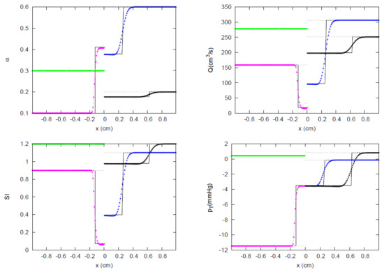
Figure 62. Section 3.3. Test 4V17. Comparison between analytical (—) and numerical solutions at t = 0.002 s. The solution of test case 4V17 from vessels 1 to 4 is: a subsonic BCW, a supersonic flow entering the confluence, a supersonic FDW, and a supersonic FDW, respectively. Vessels 1, 3, and 4 share the same value of $p_T$ at $x=0$.

In test case 4V18 (Figure 63), subsonic/supersonic initial conditions are imposed in vessels 1,4/2,3, respectively. In the solution, while merging-flow vessel 2 preserves its initial condition, the rest of the vessels share a constant level of energy at the junction under conditions of subsonic flow.

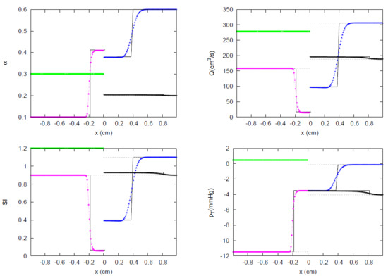
Figure 63. Section 3.3. Test 4V18. Comparison between analytical (—) and numerical solutions at t = 0.003 s. The solution of test case 4V18 from vessels 1 to 4 is: a subsonic BCW, a supersonic flow entering the confluence, a supersonic FDW, and a subsonic FCW, respectively. Vessels 1, 3, and 4 share the same value of $p_T$ at $x=0$.

Subsonic/supersonic initial conditions are imposed in vessels 1,4/2,3, respectively, in test case 4V19 (Figure 64), but with setting $u<0$. Vessel 3 preserves its supersonic initial condition and does not participate in the energy level at the junction. The rest of the vessels share a constant level of energy at the junction under conditions of subsonic flow.

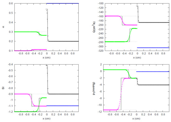
Figure 64. Section 3.3. Test 4V19. Comparison between analytical (—) and numerical solutions at t = 0.001 s. The solution of test case 4V19 from vessels 1 to 4 is: a supersonic BCW, a supersonic BDW, a supersonic flow entering the confluence, and a subsonic FCW, respectively. Vessels 1, 2, and 4 share the same value of $p_T$ at $x=0$.

In test case 4V20 (Figure 65), the flow in vessels 1 and 4 is initially subsonic with $u>0$, while the flow in vessels 2 and 3 is initially supersonic with $u<0$. Flow in vessel 2 does not change over time. A supersonic BCW is generated in vessel 1 departing from subsonic conditions. A supersonic FDW and a subsonic FCW appear in vessels 3 and 4 respectively. Vessels 1, 3 and 4, even showing different conditions for the $SI$ at $x=0$, share the same level of energy at the junction.

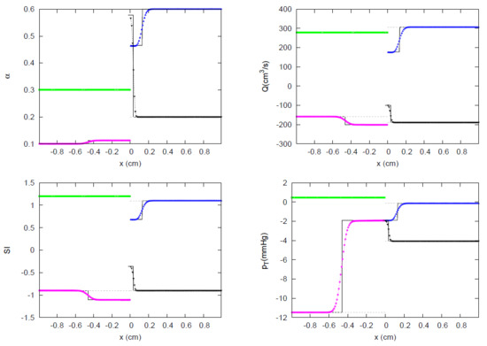
Figure 65. Section 3.3. Test 4V20. Comparison between analytical (—) and numerical solutions at t = 0.001 s. The solution of test case 4V20 from vessels 1 to 4 is: a supersonic BCW, a supersonic flow entering the confluence, a supersonic FDW, and a subsonic FCW, respectively. Vessels 1, 3, and 4 share the same value of $p_T$ at $x=0$.

The flow in vessels 1 and 4 is initially supersonic with $u<0$, while the flow in vessels 2 and 3 is initially subsonic with $u>0$, in test case 4V21 (Figure 66). Subsonic conditions for vessels 1 and 2 and supersonic conditions for vessel 3 are generated at the junction, under the same level of $p_T$. The flow in Vessel 4 remains unaltered over time.

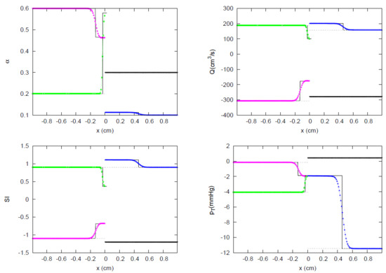
Figure 66. Section 3.3. Test 4V21. Comparison between analytical (—) and numerical solutions at t = 0.001 s. The solution of test case 4V21 from vessels 1 to 4 is: a supersonic BDW, a subsonic BCW, a supersonic FCW, and a supersonic flow entering the confluence, respectively. Vessels 1, 2, and 3 share the same value of $p_T$ at $x=0$.

In test case 4V22 (Figure 67), supersonic initial conditions are imposed in all vessels, leading to a supersonic BCW and supersonic FDW for vessels 1 and 2 respectively, sharing the same level of $p_T$ at $x=0$. Vessels 1 and 4 remain unaltered over time.

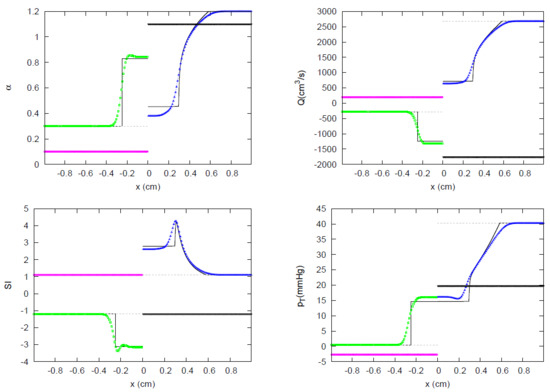
Figure 67. Section 3.3. Test 4V22. Comparison between analytical (—) and numerical solutions at t = 0.001 s. The solution of test case 4V22 from vessels 1 to 4 is: a supersonic flow entering the confluence, a supersonic BCW, a supersonic FDW, and a supersonic flow entering the confluence, respectively. Vessels 2 and 3 share the same value of $p_T$ at $x=0$.

Zero velocity conditions are prescribed in vessel 2, while supersonic conditions are imposed in vessels 1,2 and 4, in test case 4V23 (Figure 68). Solution in vessel 2, a BDW, generates sonic flow conditions at the junction, while supersonic initial flow conditions in vessel 1 remains unaltered over time. Both vessels 1 and 2 provide mass to vessels 3 and 4, where suction has been initially imposed. Flow in vessels 3 and 4 evolves from supersonic to subsonic conditions along an FDW and they share the same level of energy at the junction. It can also be clearly seen that for vessels 3 and 4, the $SI$ does not show a monotonically decreasing variation between the initial and the solution region. The maximum value of $SI$ appears when the vessel deformation becomes equal to ${\alpha }_{min}$ during the expansion fan.

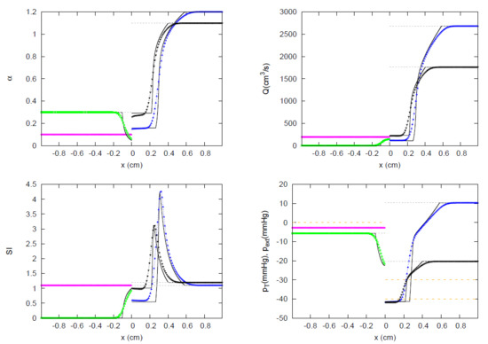
Figure 68. Section 3.3. Test 4V23. Comparison between analytical (—) and numerical solutions at t = 0.001 s. The solution of test case 4V23 from vessels 1 to 4 is: a supersonic flow entering the confluence, a subsonic BDW including sonic limitation, a supersonic FDW, and a supersonic FDW, respectively. Vessels 3 and 4 share the same value of $p_T$ at $x=0$.

Test cases 4V24 to test case 4V27 are cases where collapsed areas are imposed in all vessels. Test case 4V23 is modified by imposing collapsed areas for vessels 3 and 4, leading to JRP 4V24 (Figure 69). Solutions for vessel 1 and 2, supersonic flow entering the confluence and a subsonic BDW including flow limitation, do not participate in the energy conservation equation. The initial conditions of the JRP generate an FDW for both vessels 3 and 4, and share the same level of $p_T$ at $x=0$ under conditions of subsonic flow.

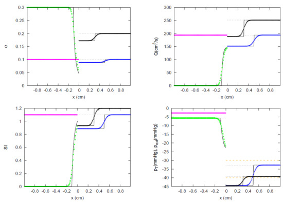
Figure 69. Section 3.3. Test 4V24. Comparison between analytical (—) and numerical solutions at t = 0.001 s. The solution of test case 4V24 from vessels 1 to 4 is: a supersonic flow entering the confluence, a subsonic BDW including sonic limitation, a supersonic FDW, and a supersonic FDW, respectively. Vessels 3 and 4 share the same value of $p_T$ at $x=0$.

Initial conditions in test case 4V25 (Figure 70) ensure that all vessels are flow merging vessels. The solution is a supersonic flow entering the confluence for vessels 2 and 3 (unaltered over time), a subsonic BDW including sonic limitation for vessel 1 and a subsonic FCW for vessels 4, where a large jump in vessel area is observed. As a consequence, all vessels provide a different value of total pressure preserved at $x=0$.

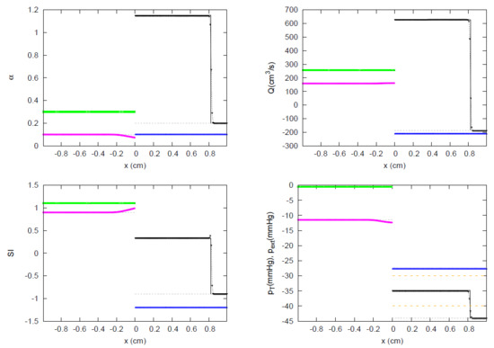
Figure 70. Section 3.3. Test 4V25. Comparison between analytical (—) and numerical solutions at t = 0.007 s. The solution of test case 4V25 from vessels 1 to 4 is: a subsonic BDW including sonic limitation, a supersonic flow entering the confluence, a supersonic flow entering the confluence, and a subsonic FCW, respectively. Total pressure is not preserved at $x=0$.

Again, all vessels are flow merging vessels in test case 4V26 (Figure 71). The solution is a supersonic flow entering the confluence for vessels 1 and 4 (unaltered over time), a subsonic BDW including sonic limitation for vessel 2 and a subsonic FCW for vessels 3, where now an expansion in vessel area is present. Total pressure is not preserved at $x=0$.

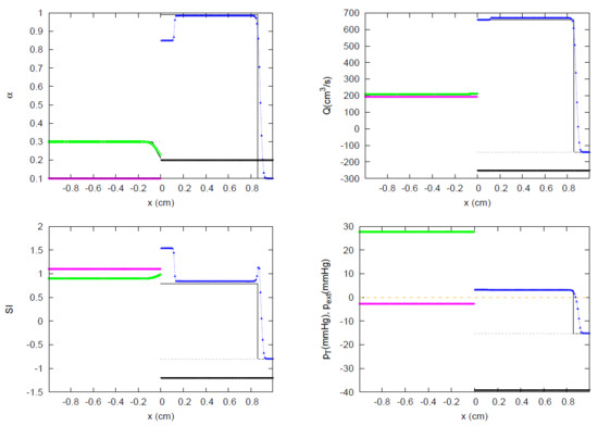
Figure 71. Section 3.3. Test 4V26. Comparison between analytical (—) and numerical solutions at m. The solution of test case 4V26 from vessels 1 to 4 is: a supersonic flow entering the confluence, a subsonic BDW including sonic limitation, a subsonic FCW, and a supersonic flow entering the confluence, respectively. Total pressure is not preserved at $x=0$.

Initial conditions in test case 4V27 (Figure 72) generate a vacuum state in the neighborhood of the junction. All solutions are decompression waves ending in a subsonic state at $x=0$, where all vessels share the same value of total pressure at $x=0$.

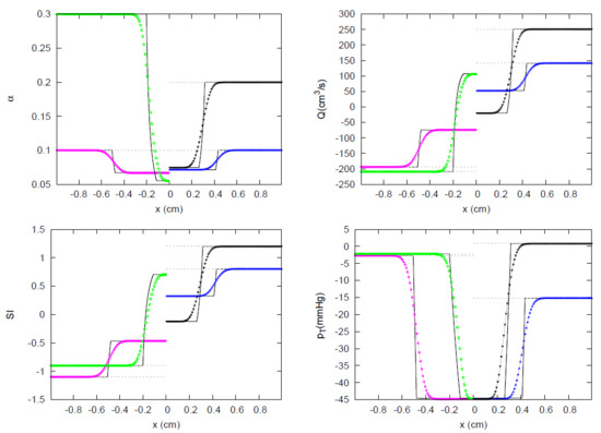
Figure 72. Section 3.3. Test 4V27. Comparison between analytical (—) and numerical solutions at t = 0.001 s. The solution of test case 4V27 from vessels 1 to 4 is: a supersonic BDW, a subsonic BDW, a subsonic FDW, and a supersonic FDW, respectively. All vessels share the same value of $p_T$ at $x=0$.

4. Conclusions

In the current work, a methodology for the solution of the Junction Riemann Problem for 1D hyperbolic balance laws in networks of elastic vessels has been proposed. The solver presented can deal with all possible transitions of flow, including flow limitation and supersonic flow conditions on elastic collapsible tubes. Solutions are based on rarefaction waves or shock waves that are completely consistent with the underlying hyperbolic system of conservation laws. The resulting JRP solver can be used in combination with any numerical scheme of an arbitrary order of accuracy.

The methodology has been illustrated in test cases with discontinuous variations of mechanical and geometrical properties of vessels and compared with exact solutions in junctions with two vessels, showing the expected limitations of the JRP solver presented in this work, where solutions in each branch of the confluence only contain at most one type of wave. The solutions satisfy, in all cases, the entropy conditions for shocks or rarefactions for both subsonic and supersonic conditions. The solver has also been tested in junctions with three and four vessels, considering merging flows, splitting flows or any other possible combination in a confluence of vessels under subsonic and supersonic conditions.

The solution method is based on an iterative search of the solution, and the computational details used in this work have been detailed. Convergence to suitable solutions has been assessed in a variety of cases. In all cases, analytical solutions of the proposed JRP solver and numerical solutions generated by combining the JRP methodology with the HLLS are presented. In all cases, convergence to the solution is guaranteed, including cases with collapsed states, subsonic–supersonic transitions, sonic blockage conditions, and the transmission of backward waves from downstream vessels through the junction to upstream supersonic vessels with supersonic conditions.

References

- Bellamoli, F.; Müller, L.O.; Toro, E.F. A numerical method for junctions in networks of shallow-water channels. Appl. Math. Comput. 2018, 337, 190–213. [Google Scholar] [CrossRef] [Green Version]
- Wang, J.; Parker, K. Wave propagation in a model of the arterial circulation. J. Biomech. 2004, 37, 457–470. [Google Scholar] [CrossRef]
- Xiao, N.; Alastruey, J.; Alberto Figueroa, C. A systematic comparison between 1-D and 3-D hemodynamics in compliant arterial models. Int. J. Numer. Methods Biomed. Eng. 2014, 30, 204–231. [Google Scholar] [CrossRef] [Green Version]
- Morgan, P.; Parker, K. A mathematical model of flow through a collapsible tube—I. Model and steady flow results. J. Biomech. 1989, 22, 1263–1270. [Google Scholar] [CrossRef]
- Pedley, T.; Luo, X. Modelling flow and oscillations in collapsible tubes. Theor. Comput. Fluid Dyn. 1998, 10, 277–294. [Google Scholar] [CrossRef]
- Bassez, S.; Flaud, P.; Chauveau, M. Modeling of the deformation of flexible tubes using a single law: Application to veins of the lower limb in man. J. Biomech. Eng. 2001, 123, 58–65. [Google Scholar] [CrossRef]
- Marchandise, E.; Flaud, P. Accurate modelling of unsteady flows in collapsible tubes. Comput. Methods Biomech. Biomed. Eng. 2010, 13, 279–290. [Google Scholar] [CrossRef]
- Ho, H.; Mithraratne, K.; Hunter, P. Numerical Simulation of Blood Flow in an Anatomically-Accurate Cerebral Venous Tree. IEEE Trans. Med. Imaging 2013, 32, 85–91. [Google Scholar] [CrossRef]
- Müller, L.O.; Toro, E.F. A global multiscale mathematical model for the human circulation with emphasis on the venous system. Int. J. Numer. Methods Biomed. Eng. 2014, 30, 681–725. [Google Scholar] [CrossRef] [PubMed]
- Müller, L.O.; Toro, E.F. Enhanced global mathematical model for studying cerebral venous blood flow. J. Biomech. 2014, 47, 3361–3372. [Google Scholar] [CrossRef] [PubMed]
- Mynard, J.P.; Smolich, J.J. One-Dimensional Haemodynamic Modeling and Wave Dynamics in the Entire Adult Circulation. Ann. Biomed. Eng. 2015, 43, 1443–1460. [Google Scholar] [CrossRef]
- Elshobaki, M.; Valiani, A.; Caleffi, V. Numerical modelling of open channel junctions using the Riemann problem approach. J. Hydraul. Res. 2019, 57, 662–674. [Google Scholar] [CrossRef]
- Zhang, X.; Noda, S.; Himeno, R.; Liu, H. Gravitational effects on global hemodynamics in different postures: A closed-loop multiscale mathematical analysis. Acta Mech. Sin. 2017, 33, 595–618. [Google Scholar] [CrossRef]
- Sherwin, S.; Franke, V.; Peiró, J.; Parker, K. One-dimensional modelling of a vascular network in space-time variables. J. Eng. Math. 2003, 47, 217–250. [Google Scholar] [CrossRef]
- Sherwin, S.J.; Formaggia, L.; Peiró, J.; Franke, V. Computational modelling of 1D blood flow with variable mechanical properties and its application to the simulation of wave propagation in the human arterial system. Int. J. Numer. Methods Fluids 2003, 43, 673–700. [Google Scholar] [CrossRef]
- Joseph, E. Flaherty, J.B.K.; Rubinow, S.I. Post Buckling Behavior of Elastic Tubes and Rings with Opposite Sides in Contact. SIAM J. Appl. Math. 1972, 23, 446–455. [Google Scholar] [CrossRef]
- Elad, D.; Katz, D.; Kimmel, E.; Einav, S. Numerical schemes for unsteady fluid flow through collapsible tubes. J. Biomed. Eng. 1991, 13, 10–18. [Google Scholar] [CrossRef]
- Brook, B.; Pedley, T. A model for time-dependent flow in (giraffe jugular) veins: Uniform tube properties. J. Biomech. 2002, 35, 95–107. [Google Scholar] [CrossRef]
- Quarteroni, A.; Formaggia, L. Mathematical Modelling and Numerical Simulation of the Cardiovascular System. In Computational Models for the Human Body; Elsevier: Amsterdam, The Netherlands, 2004; Volume 12, pp. 3–127. [Google Scholar] [CrossRef]
- Miglio, E.; Perotto, S.; Saleri, F. Model coupling techniques for free-surface flow problems: Part I. Nonlinear Anal. Theory Methods Appl. 2005, 63, e1885–e1896. [Google Scholar] [CrossRef]
- Bermúdez, A.; López, X.; Vázquez-Cendón, M.E. Treating network junctions in finite volume solution of transient gas flow models. J. Comput. Phys. 2017, 344, 187–209. [Google Scholar] [CrossRef]
- Fullana, J.M.; Zaleski, S. A branched one-dimensional model of vessel networks. J. Fluid Mech. 2009, 621, 183–204. [Google Scholar] [CrossRef]
- Huang, P.G.; Muller, L.O. Simulation of one-dimensional blood flow in networks of human vessels using a novel TVD scheme. Int. J. Numer. Methods Biomed. Eng. 2015, 31, e02701. [Google Scholar] [CrossRef]
- Müller, L.O.; Blanco, P.J. A high order approximation of hyperbolic conservation laws in networks: Application to one-dimensional blood flow. J. Comput. Phys. 2015, 300, 423–437. [Google Scholar] [CrossRef]
- Toro, E.F.; Siviglia, A. Flow in Collapsible Tubes with Discontinuous Mechanical Properties: Mathematical Model and Exact Solutions. Commun. Comput. Phys. 2013, 13, 361–385. [Google Scholar] [CrossRef]
- Toro, E. Riemann Solvers and Numerical Methods for Fluid Dynamics, 3rd ed.; Springer: Berlin/Heidelberg, Germany, 2009. [Google Scholar]
- Murillo, J.; García-Navarro, P. Augmented versions of the HLL and HLLC Riemann solvers including source terms in one and two dimensions for shallow flow applications. J. Comput. Phys. 2012, 231, 6861–6906. [Google Scholar] [CrossRef]
- Murillo, J.; Navas-Montilla, A.; García-Navarro, P. Formulation of exactly balanced solvers for blood flow in elastic vessels and their application to collapsed states. Comput. Fluids 2019, 186, 74–98. [Google Scholar] [CrossRef]
- Harten, A.; Lax, P.D.; Leer, B.V. On Upstream Differencing and Godunov-Type Schemes for Hyperbolic Conservation Laws. SIAM Rev. 1983, 25, 35–61. [Google Scholar] [CrossRef]
- Murillo, J.; García-Navarro, P. A Roe type energy balanced solver for 1D arterial blood flow and transport. Comput. Fluids 2015, 117, 149–167. [Google Scholar] [CrossRef]
- LeVeque, R.J. Balancing Source Terms and Flux Gradients in High-Resolution Godunov Methods: The Quasi-Steady Wave-Propagation Algorithm. J. Comput. Phys. 1998, 146, 346–365. [Google Scholar] [CrossRef] [Green Version]
- LeVeque, R.J. Finite-Volume Methods for Hyperbolic Problems; Cambridge University Press: Cambridge, UK, 2002. [Google Scholar]
- Murillo, J.; García-Navarro, P. Weak solutions for partial differential equations with source terms: Application to the shallow water equations. J. Comput. Phys. 2010, 229, 4327–4368. [Google Scholar] [CrossRef]
- Murillo, J.; García-Navarro, P. Energy balance numerical schemes for shallow water equations with discontinuous topography. J. Comput. Phys. 2013, 236, 119–142. [Google Scholar] [CrossRef]
- Thompson, K.W. Time-dependent boundary conditions for hyperbolic systems, II. J. Comput. Phys. 1990, 89, 439–461. [Google Scholar] [CrossRef]
Publisher’s Note: MDPI stays neutral with regard to jurisdictional claims in published maps and institutional affiliations. |
© 2021 by the authors. Licensee MDPI, Basel, Switzerland. This article is an open access article distributed under the terms and conditions of the Creative Commons Attribution (CC BY) license (https://creativecommons.org/licenses/by/4.0/).