Symplectic-Structure-Preserving Uncertain Differential Equations

Abstract

Uncertain differential equations are important mathematical models in uncertain environments. This paper investigates uncertain multi-dimensional and multiple-factor differential equations. First, the solvability of the equations is analyzed. The $\alpha$-path distributions and expected values of solutions are given. Then, structure preserving uncertain differential equations, uncertain Hamiltonian systems driven by Liu processes, which possess a kind of uncertain symplectic structures, are presented. A symplectic scheme with six-order accuracy and a Yao-Chen algorithm are applied to design an algorithm to solve uncertain Hamiltonian systems. At last, numerical experiments are given to investigate four uncertain Hamiltonian systems, which highlight the efficiency of our algorithm.

1. Introduction

An uncertain differential equation (abbreviated as UDE) is a kind of mathematical model to describe physical processes in uncertain environments [1,2,3]. To model human belief degree, on the basis of normality, subadditivity and product axioms, uncertain theory is introduced elaborately in [1]. A product axiom defining uncertain measures in uncertain theory is the essential difference from probability theory. Probability theory is suitable for big data analysis, while uncertain theory is appropriate for the situation of fewer data information. Subsequently, UDE theory is expounded in [2,3]. UDE is driven by the Liu process. As a counterpart of Wiener process, the Liu process can be used to deal with white noise [1,2,3]. The Liu process is stationary and has independent normal increment. More specifically, it almost certainly possesses Lipschitz continuous sample paths. In the UDE model, the noise term can be seen as a normal uncertain variable with an expected value of 0 and variance of 1. Refs. [4,5,6] investigate the well-posedness of some UDEs. Refs. [7,8,9,10,11,12] analyze asymptotic stability, stability in mean, moment exponential stability, almost sure stability, exponential stability and stability in distribution of UDEs. Analytic solutions of some UDEs are studied in [13,14,15,16], while numerical investigations are developed in [17,18,19,20,21,22,23], such as the Euler method, Runge–Kutta methods, Adams methods, Milne method, Hamming method and difference method. Since it is hard to obtain exact solutions of UDEs in practice, numerical analysis is very important for applications of UDEs [24].

Stochastic Hamiltonian systems, as a kind of structure-preserving stochastic differential equations, are used to simulate dynamic systems under stochastic dissipative disturbance [25,26,27,28,29,30]. If the disturbances are seen as white noise, stochastic Hamiltonian systems can be written as stochastic differential equations driven by Wiener processes. Since stochastic Hamiltonian systems possess symplectic geometric structures and symmetries, they are used to describe approximately conservative physical processes in some cases. However, in other practical cases, the stochastic Hamiltonian system model is imperfect for empirical analysis. An illustrative example is given in Appendix A. In modeling real dynamic systems in uncertain environments, it is more reasonable to treat dissipative disturbances as uncertain factors. Whether from the perspective of completeness of mathematical research or from the perspective of providing new models for different application problems, it makes sense to study uncertain dynamic systems with symplectic geometric structures.

So, in this paper, based on the Liu process, we present uncertain Hamiltonian system models. Similarly to stochastic counterparts, uncertain Hamiltonian systems possess uncertain symplectic structures and symmetries and can imply some essential physical property of uncertain dynamic systems. The contribution of this paper is as follows.

• We present a kind of symplectic-structure-preserving UDE, an uncertain Hamiltonian system. We prove the structure-preserving property of uncertain Hamiltonian system. It is a good supplement to the model of stochastic Hamiltonian systems;
• We analyze the well-posedness and $\alpha -$path distributions of general $2m-$dimension and $n-$factor UDEs. Naturally, under the Lipschitz continuity and linear growth condition, the uncertain Hamiltonian system is well-posed. With $\alpha -$paths, the inverse uncertainty distribution of uncertain Hamiltonian system can be obtained;
• We give an algorithm by applying a symplectic scheme with high precision and Yao-Chen algorithm to solve $\alpha -$path solutions and expected values of uncertain Hamiltonian systems. We also carry out numerical experiments to test the effectiveness of the algorithm.

The rest of this paper is arranged as follows. In Section 2, we investigate the well-posedness and $\alpha$-path distributions of a kind of $2m-$dimension and n-factor UDEs. In Section 3, an uncertain Hamiltonian system is presented. We evidence the structure-preserving property of uncertain Hamiltonian systems. An algorithm is also given to compute $\alpha$-path solutions and expected values of uncertain Hamiltonian systems. A numerical experiment is carried out in Section 4 to confirm the effectiveness of our algorithm. The conclusion is given in Section 5. In Appendix A, we list a paradox of stochastic Hamiltonian systems in one case.

2. Multi-Dimensional and Multiple-Factor UDE

In this paper, we consider the following initial value problem of $2m$-dimension and n-factor UDE

$$\begin{array}{c}\hfill \begin{array}{c}d{U}_t=f(t,U_t,V_t)dt+\sum _{k=1}^n{\sigma }_k(t,U_t,V_t)d{C}_{kt},\hfill \\ d{V}_t=g(t,U_t,V_t)dt+\sum _{k=1}^n{\rho }_k(t,U_t,V_t)d{C}_{kt},\hfill \\ U_{t_0}=U_0,V_{t_0}=V_0,\hfill \end{array}\end{array}$$

(1)

where $U_t,V_t,f,g,{\sigma }_k,{\rho }_k,C_{kt}$ are m-dimension vectors with components

$$U_t^j,V_t^j,f^j,g^j,{\sigma }_k^j,{\rho }_k^j,C_{kt}^j,j=1,\dots ,m,k=1,\dots ,n,$$

respectively. Assume that $f,g,{\sigma }_k,{\rho }_k$ are appropriately smooth functions. Here, $C_{kt},k=1,\dots ,n,$ are independent $m-$dimensional Liu processes. They are Lipschitz continuous processes with independent and stationary increments to describe uncertain white noises [1,2,3]. Every increment $C_{k(t+s)}^j-C_{ks}^j$ is a normal uncertain variable with an uncertain distribution [1,2,3]

$${\mathsf{\Phi }}_t(x)={\left(1+exp\left(-\frac{\pi x}{\sqrt{3}t}\right)\right)}^{-1},x\in R,t,s\ge 0.$$

(2)

Remark 1.

The basic differences of the Liu process $C_t$ from the Wiener process $W_t$ are as follows.

(1) 

Increment $C_{t+s}-C_s$ of Liu process $C_t$ obeys normal uncertain distribution (2), while for the Wiener process, $W_{t+s}-W_s$ is $N(0,t)$.

(2) 

Almost all sample paths of the Liu process are Lipschitz continuous, while for Wiener process, the sample path is not Lipschitz continuous; it is uniformly Hölder continuous for each exponent $\gamma <1/2,$ but is not Hölder continuous with any exponent $\gamma >1/2$.

(3) 

The uncertain white noise ${\dot{C}}_t$ can be seen as a normal uncertain variable with an expected value of 0 and variance of 1, while the stochastic white noise ${\dot{W}}_t$ a normal random variable with an expected value of 0 and variance of 1/dt.

Similarly to the proof of Theorem 4.1, in [4], by applying Lemma 4.1 in [4], we prove the following well-posedness proposition.

Proposition 1.

Let $f,g,{\sigma }_k,{\rho }_k,k=1,\dots ,n,$ be functions with three variables. Assume that $C_{kt},k=1,\dots ,n,$ are independent $m-$dimensional Liu processes. Under the following Lipschitz continuity and linear growth condition

$$\begin{array}{c}\hfill \begin{array}{c}\sum _{k=1}^n|{\sigma }_k(t,u,v)-{\sigma }_k(t,\overline{u},\overline{v})|+|{\rho }_k(t,u,v)-{\rho }_k(t,\overline{u},\overline{v})|\hfill \\ +|f(t,u,v)-f(t,\overline{u},\overline{v})|+|g(t,u,v)-g(t,\overline{u},\overline{v})|\le L(|u-\overline{u}|+|v-\overline{v}|),\hfill \\ \left|f(t,u,v)\right|+\left|g(t,u,v)\right|+\sum _{k=1}^n|{\sigma }_k(t,u,v)|+|{\rho }_k(t,u,v)|\le L(1+\left|u\right|+\left|v\right|),\hfill \end{array}\end{array}$$

the uncertain system (1) is solvable uniquely and satisfies sample-continuity.

Proof of Proposition 1. 

Let $U_t^{(0)}=U_0,V_t^{(0)}=V_0.$ Define iterative sequences as follows

$$U_t^{(n)}=U_0+{\int }_{t_0}^{t}f(s,U_s^{(n-1)},V_s^{(n-1)})ds+\sum _{k=1}^n{\int }_{t_0}^t{\sigma }_k(s,U_s^{(n-1)},V_s^{(n-1)})d{C}_{ks},$$

$$V_t^{(n)}=V_0+{\int }_{t_0}^{t}g(s,U_s^{(n-1)},V_s^{(n-1)})ds+\sum _{k=1}^n{\int }_{t_0}^t{\rho }_k(s,U_s^{(n-1)},V_s^{(n-1)})d{C}_{ks}.$$

Denote $D_t^n={max}_{t_0\le s\le t}\left\{\right|U_s^{(n+1)}-U_s^{(n)}|,|V_s^{(n+1)}-V_s^{(n)}\left|\right\}$. For each sample $\gamma$, let $K_{\gamma }$ be the sum of Lipschitz constants $K_{\gamma }^k$ for $C_{kt},k=1,\dots ,n.$ First, we have

$$\begin{array}{c}\hfill \begin{array}{c}|U_t^{(1)}-U_t^{(0)}|\le {\int }_{t_0}^t|f(s,U_0,V_0)|ds+\sum _{k=1}^n{K}_{\gamma }^k{\int }_{t_0}^t\left|{\sigma }_k(s,U_0,V_0)\right|ds\hfill \\ \le (1+|U_0|+|V_0|)\left[L(1+K_{\gamma })\right](t-t_0).\hfill \end{array}\end{array}$$

Similarly, we obtain $|V_t^{(1)}-V_t^{(0)}|\le (1+|U_0|+|V_0|)\left[L(1+K_{\gamma })\right](t-t_0).$ Therefore, we obtain

$$D_t^0\le (1+|U_0|+|V_0|)\left[L(1+K_{\gamma })\right](t-t_0).$$

Second, we derive

$$\begin{array}{c}\hfill \begin{array}{c}|U_t^{(n+1)}-U_t^{(n)}|\le {\int }_{t_0}^t|f(s,U_s^{(n)},V_s^{(n)})-f(s,U_s^{(n-1)},V_s^{(n-1)})|ds\hfill \\ +\sum _{k=1}^n{K}_{\gamma }^k{\int }_{t_0}^t|{\sigma }_k(s,U_s^{(n)},V_s^{(n)})-{\sigma }_k(s,U_s^{(n-1)},V_s^{(n-1)})|ds\hfill \\ \le \left[L(1+K_{\gamma })\right]{\int }_{t_0}^t{D}_s^{n-1}ds.\hfill \end{array}\end{array}$$

Similarly, we have $|V_t^{(n+1)}-V_t^{(n)}|\le \left[L(1+K_{\gamma })\right]{\int }_{t_0}^t{D}_s^{n-1}ds.$ This implies that

$$D_t^n\le \left[L(1+K_{\gamma })\right]{\int }_{t_0}^t{D}_s^{n-1}ds.$$

By mathematical induction, we derive

$$\begin{array}{c}\hfill \begin{array}{c}{D}_t^n\le (1+|U_0|+|V_0|)\frac{{\left[L(1+K_{\gamma })\right]}^{n+1}}{(n+1)!}{(t-t_0)}^{n+1},\hfill \\ \sum _{n=0}^{+\infty }{D}_t^n\le (1+|U_0|+|V_0|)exp\left[L(1+K_{\gamma })(t-t_0)\right].\hfill \end{array}\end{array}$$

(3)

According to the Weierstrass criterion, the inequality (3) ensures that $U_t^{(n)},V_t^{(n)}$ converge uniformly for $t\in [t_0,T].$ Denote their limits by $U_t,V_t.$ Then, by uniform convergence and integrality, we obtain

$$\begin{array}{c}\hfill \begin{array}{c}{U}_t=U_0+{\int }_{t_0}^{t}f(s,U_s,V_s)ds+\sum _{k=1}^n{\int }_{t_0}^t{\sigma }_k(s,U_s,V_s)d{C}_{ks},\hfill \\ V_t=V_0+{\int }_{t_0}^{t}g(s,U_s,V_s)ds+\sum _{k=1}^n{\int }_{t_0}^t{\rho }_k(s,U_s,V_s)d{C}_{ks}.\hfill \end{array}\end{array}$$

(4)

The above integral form is equivalent to the uncertain system (1).

Suppose that system (1) has two solutions $U_t,V_t$ and ${\tilde{U}}_t,{\tilde{V}}_t$. Then, we obtain

$$|U_t-{\tilde{U}}_t|\le \left[L(1+K_{\gamma })\right]{\int }_{t_0}^t|U_s-{\tilde{U}}_s|ds,$$

$$|V_t-{\tilde{V}}_t|\le \left[L(1+K_{\gamma })\right]{\int }_{t_0}^t|V_s-{\tilde{V}}_s|ds.$$

The Gronwall inequality yields $U_t={\tilde{U}}_t,V_t={\tilde{V}}_t.$ Thus, system (1) is uniquely solvable.

The inequality (3) ensures that $U_t,V_t$ are bounded by $2(1+|U_0|+|V_0|)exp\left[L(1+K_{\gamma })(t-t_0)\right].$ Assume that $t_0\le \tau \le t.$ We derive

$$\begin{array}{c}\hfill \begin{array}{c}|U_t-U_{\tau }|=|{\int }_{\tau }^{t}f(s,U_s,V_s)ds+\sum _{k=1}^n{\int }_{\tau }^t{\sigma }_k(s,U_s,V_s)d{C}_{ks}|\hfill \\ \le \left[L(1+K_{\gamma })\right]{\int }_{\tau }^t(1+|U_s|+|V_s|)ds\hfill \\ \le 5(1+|U_0|+|V_0|)\left[L(1+K_{\gamma })\right]exp\left[L(1+K_{\gamma })(t-t_0)\right](t-\tau ).\hfill \end{array}\end{array}$$

(5)

Therefor, $U_{\tau }\to U_t$ as $\tau \to t.$ Similarly, $V_t$ also has sample-continuity.  □

In many cases, it is difficult to find an analytical solution or its uncertain distribution of a general UDE (1). Alternatively, the solution of a UDE can be represented by that of a spectrum of deterministic systems, which is called $\alpha -$paths [1,2,3,17,18,19,20,21,22,23]. Yao-Chen formula in [3] relates UDEs and deterministic systems, just like the Feynman-Kac formula relates stochastic differential equations and deterministic systems. $\alpha -$paths provide a method to solve a UDE. So according to Yao-Chen formula, Yao-Chen algorithm is designed to solve UDEs numerically [3].

Below, according to [1,2,3,17,18,19,20,21,22,23], we define $\alpha$-path solutions $U_t^{\alpha },V_t^{\alpha }$ of the system (1) as solutions of the following deterministic system

$$\begin{array}{c}\hfill \begin{array}{c}d{U}_t^{\alpha }=f(t,U_t^{\alpha },V_t^{\alpha })dt+\sum _{k=1}^n\left|{\sigma }_k(t,U_t^{\alpha },V_t^{\alpha })\right|{\mathsf{\Phi }}^{-1}(\alpha )dt,\hfill \\ d{V}_t^{\alpha }=g(t,U_t^{\alpha },V_t^{\alpha })dt+\sum _{k=1}^n\left|{\rho }_k(t,U_t^{\alpha },V_t^{\alpha })\right|{\mathsf{\Phi }}^{-1}(\alpha )dt,\hfill \end{array}\end{array}$$

(6)

where the inverse normal uncertainty distribution is

$${\mathsf{\Phi }}^{-1}(\alpha )=\sqrt{3}/\pi [ln\alpha -ln(1-\alpha )],0<\alpha <1.$$

Remark 2.

α is a stochastic parameter belonging to the open interval $(0,1)$. The α-path simply denotes the solution of Equation (6) determined for a prescribed value of α.

Remark 3.

If α is considered a prescribed real number, then Equation (6) for the numerical solution can just be treated as ordinary differential equations and not as stochastic differential equations.

Remark 4.

If some suitable Hamiltonian functions ${\overline{H}}_k(t,u,v),k=0,\dots ,n,$ exist such that

$$\begin{array}{c}\hfill \begin{array}{c}{f}^j(t,u,v)=-\partial {\overline{H}}_0/\partial v^j,g^j(t,u,v)=\partial {\overline{H}}_0/\partial u^j,j=1,\dots ,m,\hfill \\ |{\sigma }_k^j(t,u,v)|=-\partial {\overline{H}}_k/\partial v^j,\left|{\rho }_k^j(t,u,v)\right|=\partial {\overline{H}}_k/\partial u^j,k=1,\dots ,n,\hfill \end{array}\end{array}$$

(7)

then Equation (6) is an ordinary Hamiltonian system.

Similar to the Yao-Chen formula in [3], we prove the following conclusion on inverse uncertainty distributions.

Theorem 1.

Suppose that $U_t,V_t$ and $U_t^{\alpha },V_t^{\alpha }$ are the solution and $\alpha -$path of the system (1), respectively. Then,

$$\mathcal{M}\{U_t\le U_t^{\alpha },\forall t\}=\alpha ,\mathcal{M}\{U_t>U_t^{\alpha },\forall t\}=1-\alpha ,$$

$$\mathcal{M}\{V_t\le V_t^{\alpha },\forall t\}=\alpha ,\mathcal{M}\{V_t>V_t^{\alpha },\forall t\}=1-\alpha ,$$

where $\mathcal{M}$ denote the uncertain measure.

Proof of Theorem 1. 

Similar to the analyses in [1,2,3,4,5,6], we make the following notations

$$T_k^{+}=\left\{s\right|{\sigma }_k(s,U_s^{\alpha },V_s^{\alpha })\ge 0\},T_k^{-}=\left\{s\right|{\sigma }_k(s,U_s^{\alpha },V_s^{\alpha })<0\},$$

$${\mathsf{\Lambda }}_k^{+}=\left\{\gamma \right|C_{kt}^{\prime }\le {\mathsf{\Phi }}^{-1}(\alpha ),t\in T_k^{+}\},{\mathsf{\Lambda }}_k^{-}=\left\{\gamma \right|C_{kt}^{\prime }\ge {\mathsf{\Phi }}^{-1}(1-\alpha ),t\in T_k^{-}\}.$$

Then, we have $\mathcal{M}\left\{{\mathsf{\Lambda }}_k^{+}\right\}=\alpha ,\mathcal{M}\left\{{\mathsf{\Lambda }}_k^{-}\right\}=\alpha .$ For $\forall \gamma \in {\mathsf{\Lambda }}_k^{+}\bigcap {\mathsf{\Lambda }}_k^{-},\forall t,k=1,\dots ,n,$

$${\sigma }_k(t,U_t,V_t)C_{kt}^{\prime }\le \left|{\sigma }_k(t,U_t^{\alpha },V_t^{\alpha })\right|{\mathsf{\Phi }}^{-1}(\alpha ).$$

Therefore, we obtain $U_t\le U_t^{\alpha }.$ Moreover, $\mathcal{M}\{U_t\le U_t^{\alpha }\}\ge \alpha .$

Denote

$${\tilde{\mathsf{\Lambda }}}_k^{+}=\left\{\gamma \right|C_{kt}^{\prime }>{\mathsf{\Phi }}^{-1}(\alpha ),t\in T_k^{+}\},{\tilde{\mathsf{\Lambda }}}_k^{-}=\left\{\gamma \right|C_{kt}^{\prime }<{\mathsf{\Phi }}^{-1}(1-\alpha ),t\in T_k^{-}\},$$

Then, we have $\mathcal{M}\left\{{\tilde{\mathsf{\Lambda }}}_k^{+}\right\}=\mathcal{M}\left\{{\tilde{\mathsf{\Lambda }}}_k^{-}\right\}=1-\alpha .$ For $\forall \gamma \in {\tilde{\mathsf{\Lambda }}}_k^{+}\bigcap {\tilde{\mathsf{\Lambda }}}_k^{-},\forall t,k=1,\dots ,n,$

$${\sigma }_k(t,U_t,V_t)C_{kt}^{\prime }>\left|{\sigma }_k(t,U_t^{\alpha },V_t^{\alpha })\right|{\mathsf{\Phi }}^{-1}(\alpha ).$$

Therefore, we obtain $U_t>U_t^{\alpha }.$ Moreover, $\mathcal{M}\{U_t>U_t^{\alpha }\}\ge 1-\alpha .$

The duality of uncertain measure yields

$$\mathcal{M}\{U_t\le U_t^{\alpha },\forall t\}=\alpha ,\mathcal{M}\{U_t>U_t^{\alpha },\forall t\}=1-\alpha .$$

Similarly, according to systems (1) and (6), we can derive

$$\mathcal{M}\{V_t\le V_t^{\alpha },\forall t\}=\alpha ,\mathcal{M}\{V_t>V_t^{\alpha },\forall t\}=1-\alpha .$$

So, the uncertain solutions $U_t,V_t$ possess inverse uncertainty distributions $U_t^{\alpha },V_t^{\alpha }$, respectively.  □

According to similar analysis in [1,2,3,17,18,19,20,21,22,23], we can apply some numerical methods to solve inverse uncertainty distributions $U_t^{\alpha },V_t^{\alpha }$ of $U_t,V_t$, and the expected values $E{U}_t,E{V}_t$ can be computed as follows

$$E{U}_t={\int }_0^1{U}_t^{\alpha }d\alpha ,E{V}_t={\int }_0^1{V}_t^{\alpha }d\alpha .$$

3. Uncertain Hamiltonian System

Suppose that some Hamiltonian functions $H_k(t,u,v),k=0,\dots ,n,$ exist such that

$$\begin{array}{c}\hfill \begin{array}{c}{f}^j(t,u,v)=-\partial H_0/\partial v^j,g^j(t,u,v)=\partial H_0/\partial u^j,j=1,\dots ,m,\hfill \\ {\sigma }_k^j(t,u,v)=-\partial H_k/\partial v^j,{\rho }_k^j(t,u,v)=\partial H_k/\partial u^j,k=1,\dots ,n.\hfill \end{array}\end{array}$$

(8)

Then, we call the Equation (1) a $2m$-dimension n-factor uncertain Hamiltonian system. A Hamiltonian system is a dynamical system completely described by the scalar Hamiltonian functions. Similarly to stochastic Hamiltonian systems, the uncertain Hamiltonian system preserves a uncertain symplectic 2-form: $d{U}_t\wedge d{V}_t.$ The following theorem shows that an uncertain Hamiltonian system preserves a uncertain symplectic structure.

Theorem 2.

The uncertain Hamiltonian systems (1) and (8) have uncertain symplectic structures

$$d{U}_t\wedge d{V}_t=\sum _{j=1}^{m}d{U}_t^j\wedge d{V}_t^j=d{U}_0\wedge d{V}_0=\sum _{j=1}^{m}d{U_0}^j\wedge d{V_0}^j.$$

Proof. 

(Proof of Theorem 2) System (1) is rewritten formally as

$$\begin{array}{c}\hfill \begin{array}{c}{U}_t^{\prime }=f(t,U_t,V_t)+\sum _{k=1}^n{\sigma }_k(t,U_t,V_t)C_{kt}^{\prime },\hfill \\ V_t^{\prime }=g(t,U_t,V_t)+\sum _{k=1}^n{\rho }_k(t,U_t,V_t)C_{kt}^{\prime },\hfill \end{array}\end{array}$$

(9)

which yields

$${(d{U}_t\wedge d{V}_t)}^{\prime }=d{U}_t^{\prime }\wedge d{V}_t+d{U}_t\wedge d{V}_t^{\prime }=d(f+\sum _{k=1}^n{\sigma }_k{C}_{kt}^{\prime })\wedge d{V}_t+d{U}_t\wedge d(g+\sum _{k=1}^n{\rho }_k{C}_{kt}^{\prime }),$$

According to the definition of exterior differential, we have

$$d{f}^j=\sum _{i=1}^m(\partial f^j/\partial u^{i}d{U}_t^i+\partial f^j/\partial v^{i}d{V}_t^i),df\wedge d{V}_t=\sum _{j=1}^{m}d{f}^j\wedge d{V}_t^j.$$

Noting that

$$d{U}_t^j\wedge d{V}_t^i=-d{V}_t^i\wedge d{U}_t^j,d{U}_t^j\wedge d{U}_t^i=-d{U}_t^i\wedge d{U}_t^j,$$

$$d{V}_t^j\wedge d{V}_t^i=-d{V}_t^i\wedge d{V}_t^j,d{U}_t^j\wedge d{U}_t^j=d{V}_t^j\wedge d{V}_t^j=0,$$

by taking the condition (8) into account, we derive

$$\begin{array}{c}\hfill \begin{array}{c}df\wedge d{V}_t=\sum _{i,j=1}^m\partial f^j/\partial u^{i}d{U}_t^i\wedge d{V}_t^j+\partial f^j/\partial v^{i}d{V}_t^i\wedge d{V}_t^j\hfill \\ =-\sum _{i,j=1}^m\frac{{\partial }^2{H}_0}{\partial v^j\partial u^i}d{U}_t^i\wedge d{V}_t^j+\frac{{\partial }^2{H}_0}{\partial v^j\partial v^i}d{V}_t^i\wedge d{V}_t^j\hfill \\ =-\sum _{i,j=1}^m\frac{{\partial }^2{H}_0}{\partial v^j\partial u^i}d{U}_t^i\wedge d{V}_t^j.\hfill \end{array}\end{array}$$

Similarly, we obtain

$$\begin{array}{c}\hfill \begin{array}{c}d{U}_t\wedge dg=\sum _{j=1}^{m}d{U}_t^j\wedge (\sum _{i=1}^m(\partial g^j/\partial u^{i}d{U}_t^i+\partial g^j/\partial v^{i}d{V}_t^i))\hfill \\ =\sum _{i,j=1}^m\partial g^j/\partial u^{i}d{U}_t^j\wedge d{U}_t^i+\partial g^j/\partial v^{i}d{U}_t^j\wedge d{V}_t^i\hfill \\ =\sum _{i,j=1}^m\frac{{\partial }^2{H}_0}{\partial u^j\partial u^i}d{U}_t^j\wedge d{U}_t^i+\frac{{\partial }^2{H}_0}{\partial u^j\partial v^i}d{U}_t^j\wedge d{V}_t^i\hfill \\ =\sum _{i,j=1}^m\frac{{\partial }^2{H}_0}{\partial u^j\partial v^i}d{U}_t^j\wedge d{V}_t^i.\hfill \end{array}\end{array}$$

Clearly, $df\wedge d{V}_t+d{U}_t\wedge dg=0.$ By repeating the above analysis, we obtain $C_{kt}^{\prime }(d{\sigma }_k\wedge d{V}_t+d{U}_t\wedge d{\rho }_k)=0.$ Therefore, ${(d{U}_t\wedge d{V}_t)}^{\prime }=0,$ which means that $d{U}_t\wedge d{V}_t$ is an invariant. Hence, $d{U}_t\wedge d{V}_t=d{U}_0\wedge d{V}_0$.  □

Some mechanical systems can be described by vibration process. [31] studies how to determine the frequency property of nonlinear oscillator by using a Hamiltonian-based formulation. Below four uncertain Hamiltonian systems are given as counterparts of stochastic Hamiltonian systems [32], where $U_t$ and $V_t$ denote the displacement and the velocity of four oscillators under different uncertain perturbations, respectively.

Example 1.

Consider the following linear uncertain oscillator

$$\begin{array}{c}\hfill \begin{array}{c}d{U}_t=-V_{t}dt+\sigma d{C}_t,\hfill \\ d{V}_t=U_{t}dt,\hfill \\ U_0=0,V_0=1.\hfill \end{array}\end{array}$$

(10)

It is a uncertain Hamiltonian system with Hamiltonian functions

$$H_0(t,u,v)=(u^2+v^2)/2,H_1(t,u,v)=-\sigma v.$$

The Hamiltonian functions corresponding to $\alpha$-path are as follows

$${\overline{H}}_0(t,u,v)=(u^2+v^2)/2,{\overline{H}}_1(t,u,v)=-{\mathsf{\Phi }}^{-1}(\alpha )\left|\sigma \right|v.$$

Example 2.

Consider the following uncertain Kubo oscillator

$$\begin{array}{c}\hfill \begin{array}{c}d{U}_t=-a{V}_{t}dt-\sigma V_{t}d{C}_t,\hfill \\ d{V}_t=a{U}_{t}dt+\sigma U_{t}d{C}_t,\hfill \\ U_0=1,V_0=0.\hfill \end{array}\end{array}$$

(11)

It is a uncertain Hamiltonian system with Hamiltonian functions

$$H_0(t,u,v)=a(u^2+v^2)/2,H_1(t,u,v)=\sigma (u^2+v^2)/2.$$

The Hamiltonian functions corresponding to $\alpha -$path are as follows

$${\overline{H}}_0(t,u,v)=a(u^2+v^2)/2,{\overline{H}}_1(t,u,v)={\mathsf{\Phi }}^{-1}(\alpha )\left|\sigma \right|(sgn(u)u^2-sgn(v)v^2)/2.$$

Example 3.

Consider the following 2-factor linear uncertain oscillator

$$\begin{array}{c}\hfill \begin{array}{c}d{U}_t=-V_{t}dt+\delta d{C}_{1t},\hfill \\ d{V}_t=U_{t}dt+\sigma d{C}_{2t},\hfill \\ U_0=1,V_0=0.\hfill \end{array}\end{array}$$

(12)

It is a 2-factor uncertain Hamiltonian system with Hamiltonian functions

$$H_0(t,u,v)=(u^2+v^2)/2,H_1(t,u,v)=-\delta v,H_2(t,u,v)=\sigma u.$$

The Hamiltonian functions corresponding to the $\alpha$-path are as follows

$${\overline{H}}_0(t,u,v)=(u^2+v^2)/2,{\overline{H}}_1(t,u,v)=-{\mathsf{\Phi }}^{-1}(\alpha )\left|\delta \right|v,{\overline{H}}_2(t,u,v)={\mathsf{\Phi }}^{-1}(\alpha )\left|\sigma \right|u.$$

Example 4.

Consider the following 2-factor nonlinear uncertain oscillator

$$\begin{array}{c}\hfill \begin{array}{c}d{U}_t=-{\omega }^{2}sin(V_t)dt-{\sigma }_{1}cos(V_t)d{C}_{1t}-{\sigma }_{2}sin(V_t)d{C}_{2t},\hfill \\ d{V}_t=U_{t}dt,\hfill \\ U_0=0,V_0=1.\hfill \end{array}\end{array}$$

(13)

It is a 2-factor uncertain Hamiltonian system with Hamiltonian functions

$$H_0(t,u,v)=-{\omega }^{2}cosv+u^2/2,H_1(t,u,v)={\sigma }_{1}sinv,H_2(t,u,v)=-{\sigma }_{2}cosv.$$

The Hamiltonian functions corresponding to the $\alpha$-path are as follows

$${\overline{H}}_0(t,u,v)=-{\omega }^{2}cosv+u^2/2,{\overline{H}}_1(t,u,v)=-{\mathsf{\Phi }}^{-1}(\alpha )\left|{\sigma }_1\right|sgn(cosv)sinv,$$

$${\overline{H}}_2(t,u,v)={\mathsf{\Phi }}^{-1}(\alpha )\left|{\sigma }_2\right|sgn(sinv)cosv.$$

The three stage symplectic Runge–Kutta scheme with six-order accuracy applied to deterministic differential equation $y^{\prime }(x)=F(x,y)$ yields

$$\begin{array}{c}\hfill \begin{array}{c}{y}_1=y_0+\frac{h}{18}(5K_1+8K_2+5K_3),\hfill \\ K_1=F(x_0+c_{1}h,y_0+h(a_{11}{K}_1+a_{12}{K}_2+a_{13}{K}_3)),\hfill \\ K_2=F(x_0+c_{2}h,y_0+h(a_{21}{K}_1+a_{22}{K}_2+a_{23}{K}_3)),\hfill \\ K_3=F(x_0+c_{3}h,y_0+h(a_{31}{K}_1+a_{32}{K}_2+a_{33}{K}_3)),\hfill \end{array}\end{array}$$

(14)

where $c_1=1/2-\sqrt{15}/10,c_2=1/2,c_3=1/2+\sqrt{15}/10,a_{11}=a_{33}=5/16$, $a_{12}=2/9-\sqrt{15}/15$, $a_{13}=5/36-\sqrt{15}/30,a_{21}=5/36+\sqrt{15}/24,a_{22}=2/9$, $a_{23}=5/36-\sqrt{15}/24$, $a_{31}=5/36+\sqrt{15}/30,a_{32}=2/9+\sqrt{15}/15.$ Scheme (14) can be applied to solve $\alpha$-path solutions of uncertain Hamiltonian systems.

According to above analysis in Section 2, the inverse uncertain distribution and expected values could be obtained via $\alpha$-paths. In many cases, it is impossible to find the exact inverse uncertain distribution, so we need apply some appropriate numerical methods to efficiently and approximately solve the inverse uncertain distribution. On the basis of the work of [17,18,19,20,21,22,23], to simulate uncertain Hamiltonian systems (1) and (8), we design the following algorithm by applying Yao-Chen algorithm and symplectic Runge–Kutta scheme (14).

Step 1. Choose $\alpha =0.01:0.01:0.99.$

Step 2. Apply symplectic Runge–Kutta scheme (14) to deterministic system (6) and obtain $\alpha$-path solutions $U_t^{\alpha },V_t^{\alpha }$ of uncertain Hamiltonian systems (1) and (8).

Step 3. Basing on $U_t^{\alpha },V_t^{\alpha }$ we analyze uncertainty solutions $U_t,V_t$ and compute expected values $E{U}_t,E{V}_t$.

Above algorithm has high precision and preserves symplectic structure of $\alpha$-paths.

4. Numerical Results

Now, we apply the above algorithm to solve four uncertain Hamiltonian system examples in Section 3.

First, we solve Example 1.

It is easy to check that the $\alpha$-path solution of (10) is

$$U_t^{\alpha }=sin(t)(|\sigma |{\mathsf{\Phi }}^{-1}(\alpha )-1),V_t^{\alpha }=cos(t)+\left|\sigma \right|{\mathsf{\Phi }}^{-1}(\alpha )(1-cos(t)).$$

Below, we choose $\sigma =1.$

The numerical (left) vs. exact (right) trajectories of uncertain distributions for $U_t$ with $\alpha =0.2,h=0.01$ and $t\in [0,10]$ are plotted in Figure 1. Numerical (left) vs. exact (right) uncertain distributions $V_t^{\alpha }$ with $t=10,h=0.01$ and $\alpha \in (0,1)$ are depicted in Figure 2. Figure 3 shows the numerical errors of $U_t^{\alpha }$ (left) and $V_t^{\alpha }$ (right). We can see that the errors are very small. In Figure 4 and Figure 5, numerical (left) and exact (right) expected value curves $E{U}_t$ and $E{V}_t$ for $t\in [0,10]$ are drawn, respectively. As expected, the figures show that our algorithm can simulate the uncertain distributions and expected values very well. We also obtain the expectations with $t=10,h=0.01$ as follows.

$$E{U}_{10}=-0.83068,E{V}_{10}=0.53858.$$

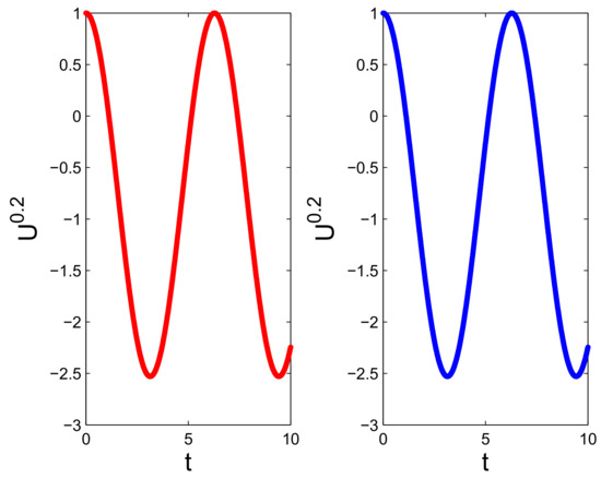
Figure 1. Trajectories of numerical (left) vs. exact (right) uncertain distributions for $U_t$ with $\alpha =0.2$, $h=0.01$ and $t\in [0,10]$.

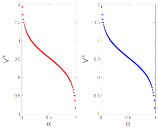
Figure 2. Numerical (left) vs. exact (right) uncertain distributions for $V_t$ with $t=10,h=0.01$ and $\alpha \in (0,1)$.

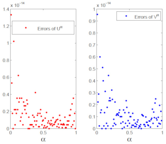
Figure 3. Numerical errors of uncertain distributions for $U_t$ (left) and $V_t$ (right) with $t=10,h=0.01$ and $\alpha \in (0,1)$.

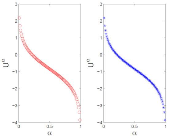
Figure 4. Numerical (left) and exact (right) expected value curves $E{U}_t$ with $t\in [0,10],h=0.01$.

Figure 5. Numerical (left) and exact (right) expected value curves $E{V}_t$ with $t\in [0,10],h=0.01$.

Second, we solve Example 2.

The $\alpha -$path solution of (11) satisfies

$$d{U}_t^{\alpha }=-a{V}_t^{\alpha }dt+\left|\sigma V_t^{\alpha }\right|{\mathsf{\Phi }}^{-1}(\alpha )dt,$$

$$d{V}_t^{\alpha }=a{U}_t^{\alpha }dt+\left|\sigma U_t^{\alpha }\right|{\mathsf{\Phi }}^{-1}(\alpha )dt.$$

Here, we choose $a=2,\sigma =0.3.$

The numerical trajectories of uncertain distributions $V_t^{\alpha }$ with $\alpha =0.4,h=0.01$ and $t\in [0,10]$ are plotted in Figure 6. Numerical uncertain distributions for $U_t$ with $t=10$, $h=0.01$ and $\alpha \in (0,1)$ are depicted in Figure 7. In Figure 8, numerical expected value curves $E{U}_t$ (left) and $E{V}_t$ (right) for $t\in [0,10]$ are drawn. We also obtain the expectations with $t=10,h=0.01$ as follows.

$$E{U}_{10}=0.56857,E{V}_{10}=0.70023.$$

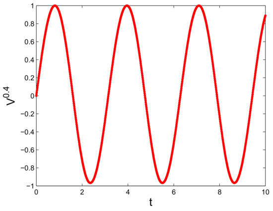
Figure 6. Trajectories of numerical uncertain distributions for $V_t$ with $\alpha =0.4,h=0.01$ and $t\in [0,10]$.

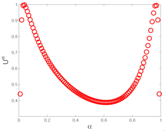
Figure 7. Numerical uncertain distributions for $U_t$ with $t=10,h=0.01$ and $\alpha \in (0,1)$.

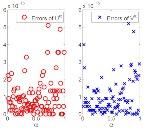
Figure 8. Expected value curves $E{U}_t$ (left) and $E{V}_t$ (right) with $t\in [0,10],h=0.01$.

Third, we solve Example 3.

It is easy to check that the $\alpha -$path solution of (12) is

$$U^{\alpha }=cos(t)+{\mathsf{\Phi }}^{-1}(\alpha )(-|\sigma |+|\sigma |cos(t)+|\gamma |sin(t)),$$

$$V^{\alpha }=sin(t)+{\mathsf{\Phi }}^{-1}(\alpha )(|\gamma |-\left|\gamma \right|cos(t)+\left|\sigma \right|sin(t)).$$

Below, we choose $\sigma =\gamma =0.5.$

The numerical (left) vs. exact (right) trajectories of uncertain distributions for $U_t$ with $\alpha =0.6,h=0.01$ and $t\in [0,10]$ are plotted in Figure 9. Numerical (left) vs. exact (right) uncertain distributions $V_t^{\alpha }$ with $t=10,h=0.01$ and $\alpha \in (0,1)$ are depicted in Figure 10. Figure 11 shows the numerical errors of $U_t^{\alpha }$ (left) and $V_t^{\alpha }$ (right). We can see that the errors are very small. In Figure 12 and Figure 13, numerical (left) and exact (right) expected value curves $E{U}_t$ and $E{V}_t$ for $t\in [0,10]$ are drawn, respectively. As expected, the figures show that our algorithm can simulate the uncertain distributions and expected values very well. We also obtain the expectations with $t=10,h=0.01$ as follows.

$$E{U}_{10}=-0.83068,E{V}_{10}=-0.53859.$$

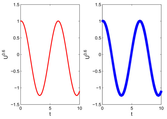
Figure 9. Trajectories of numerical (left) and exact (right) uncertain distributions for $U_t$ with $\alpha =0.6$, $h=0.01$ and $t\in [0,10]$.

Figure 10. Numerical (left) and exact (right) uncertain distributions for $V_t$ with $t=10,h=0.01$ and $\alpha \in (0,1)$.

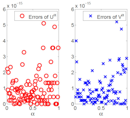
Figure 11. Numerical errors of uncertain distributions for $U_t$ (left) and $V_t$ (right) with $t=10,h=0.01$ and $\alpha \in (0,1)$.

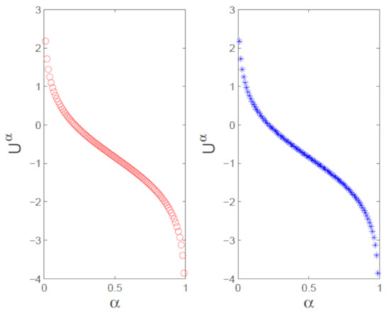
Figure 12. Numerical (left) and exact (right) expected value curves $E{U}_t$ with $t\in [0,10],h=0.01$.

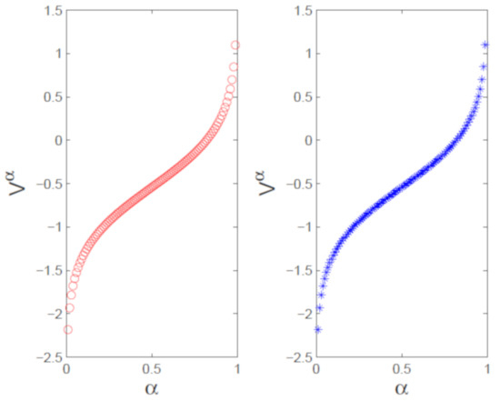
Figure 13. Numerical (left) and exact (right) expected value curves $E{V}_t$ with $t\in [0,10],h=0.01$.

At last, we solve Example 4.

The $\alpha -$path solution of (13) satisfies

$$\begin{array}{c}\hfill \begin{array}{c}d{U}_t^{\alpha }=-{\omega }^{2}sin(V_t^{\alpha })dt+(|{\sigma }_{1}cos(V_t^{\alpha })|+|{\sigma }_{2}sin(V_t^{\alpha })|){\mathsf{\Phi }}^{-1}(\alpha )dt,\hfill \\ d{V}_t^{\alpha }=U_t^{\alpha }dt.\hfill \end{array}\end{array}$$

Here, we choose ${\sigma }_1=0.2,{\sigma }_2=0.1,\omega =2.$

The numerical trajectories of uncertain distributions $V_t^{\alpha }$ with $\alpha =0.8,h=0.01$ and $t\in [0,10]$ are plotted in Figure 14. Numerical uncertain distributions for $U_t$ with $t=10$, $h=0.01$ and $\alpha \in (0,1)$ are depicted in Figure 15. In Figure 16, numerical expected value curves $E{U}_t$ (left) and $E{V}_t$ (right) for $t\in [0,10]$ are drawn. We also obtain the expectations with $t=10,h=0.01$ as follows.

$$E{U}_{10}=0.67653,E{V}_{10}=0.36315.$$

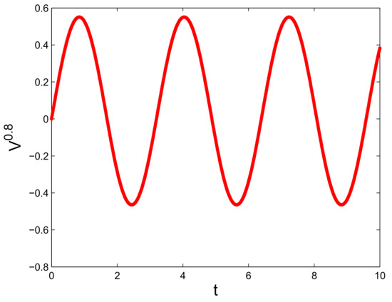
Figure 14. Trajectories of numerical uncertain distributions for $V_t$ with $\alpha =0.8,h=0.01$ and $t\in [0,10]$.

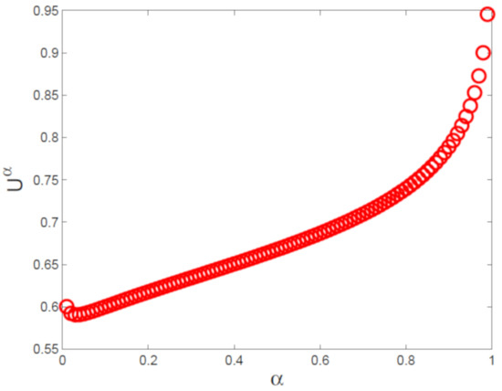
Figure 15. Numerical uncertain distributions for $U_t$ with $t=10,h=0.01$ and $\alpha \in (0,1)$.

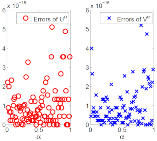
Figure 16. Expected value curves $E{U}_t$ (left) and $E{V}_t$ (right) with $t\in [0,10],h=0.01$.

5. Conclusions

This paper proposes a kind of $2m$-dimension n-factor uncertain differential equations driven by Liu processes. Under Lipschitz continuity and linear growth conditions, the uncertain systems (1) are uniquely solvable and satisfy sample-continuity. The uncertain solutions $U_t,V_t$ possess inverse uncertainty distributions $U_t^{\alpha },V_t^{\alpha }$, respectively. We can compute expected values $E{U}_t,E{V}_t$ by inverse uncertainty distributions. As a supplement of stochastic Hamiltonian systems, an uncertain Hamiltonian system is presented which presents an uncertain symplectic structure. Several examples of uncertain Hamiltonian systems are given. Numerical methods are a kind of important tools to investigate uncertain Hamiltonian systems. Symplectic Runge–Kutta scheme with six-order accuracy and Yao-Chen algorithm are applied to design an algorithm to solve inverse uncertain distributions of uncertain Hamiltonian systems and expected values of the uncertain solutions. The numerical results show the efficiency of our algorithm. For future work, applications of uncertain Hamiltonian systems could be studied, and other structure preserving generalizations, such as uncertain energy conservation systems, could be considered.

References

- Liu, B. Uncertainty Theory; Springer: Berlin/Heidelberg, Germany, 2007. [Google Scholar]
- Liu, B. Fuzzy process, hybrid process and uncertain process. J. Uncertain Syst. 2008, 2, 3–16. [Google Scholar]
- Yao, K. Uncertain Differential Equations; Springer: Berlin/Heidelberg, Germany, 2016. [Google Scholar]
- Chen, X.; Liu, B. Existence and uniqueness theorem for uncertain differential equations. Fuzzy Optim. Decis. Mak. 2010, 9, 69–81. [Google Scholar] [CrossRef]
- Ji, X.; Zhou, J. Multi-dimensional uncertain differential equation: Existence and uniqueness of solution. Fuzzy Optim. Decis. Mak. 2015, 14, 477–491. [Google Scholar] [CrossRef]
- Yang, X.; Ni, Y. Existence and uniqueness theorem for uncertain heat equation. J. Ambient. Intell. Humaniz. Comput. 2017, 8, 717–725. [Google Scholar] [CrossRef]
- Chen, X.; Gao, J. Stability analysis of linear uncertain differential equations. Ind. Eng. Manag. Syst. 2013, 12, 2–8. [Google Scholar] [CrossRef]
- Yao, K.; Ke, H.; Sheng, Y. Stability in mean for uncertain differential equation. Fuzzy Optim. Decis. Mak. 2015, 14, 365–379. [Google Scholar] [CrossRef]
- Zhu, F.; Han, Z.; Zhang, J. Moment exponential stability analysis of Markovian jump stochastic differential equations with uncertain transition jump rates. Int. J. Syst. Sci. 2015, 46, 2474–2480. [Google Scholar] [CrossRef]
- Ji, X.; Ke, H. Almost sure stability for uncertain differential equation with jumps. Soft Comput. 2016, 20, 547–553. [Google Scholar] [CrossRef]
- Sheng, Y.; Gao, J. Exponential stability of uncertain differential equation. Soft Comput. 2016, 20, 3673–3678. [Google Scholar] [CrossRef]
- Ma, W.; Liu, L.; Gao, R.; Zhang, X.; Zhang, X. Stability in distribution for multifactor uncertain differential equation. J. Ambient. Intell. Humaniz. Comput. 2017, 8, 707–716. [Google Scholar] [CrossRef]
- Jia, L.; Dai, W. Uncertain spring vibration equation. J. Ind. Manag. Optim. 2021. [Google Scholar] [CrossRef]
- Liu, Y. Semilinear uncertain differential equation with analytic solution. Information 2012, 15, 44–49. [Google Scholar]
- Wang, Z. Analytic solution for a general type of uncertain differential equation. Information 2012, 15, 153–159. [Google Scholar]
- Yao, K. A type of uncertain differential equations with analytic solution. J. Uncertain. Anal. Appl. 2013, 1, 8. [Google Scholar] [CrossRef]
- Yao, K.; Chen, X. A numerical method for solving uncertain differential equation. J. Intell. Fuzzy Syst. 2013, 25, 825–832. [Google Scholar] [CrossRef]
- Wang, X.; Ning, Y.; Moughal, T.A.; Chen, X. Adams-Simpson method for solving uncertain differential equation. Appl. Math. Comput. 2015, 271, 209–219. [Google Scholar] [CrossRef]
- Yang, X.; Ralescu, D. Adams method for solving uncertain differential equations. Appl. Math. Comput. 2015, 270, 993–1003. [Google Scholar] [CrossRef]
- Gao, R. Milne method for solving uncertain differential equations. Appl. Math. Comput. 2016, 274, 774–785. [Google Scholar] [CrossRef]
- Ji, X.; Zhou, J. Solving high-order uncertain differential equations via Runge-Kutta method. IEEE Trans. Fuzzy Syst. 2017, 1, 99–106. [Google Scholar] [CrossRef]
- Zhang, Y.; Gao, J.; Huang, Z. Hamming method for solving uncertain differential equations. Appl. Math. Comput. 2017, 313, 331–341. [Google Scholar] [CrossRef]
- Yang, X. Solving uncertain heat equation via numerical method. Appl. Math. Comput. 2018, 329, 92–104. [Google Scholar] [CrossRef]
- Shi, G.; Gao, J. European option pricing problems with fractional uncertain processes. Chaos Solitons Fractals 2021, 143, 110606. [Google Scholar] [CrossRef]
- Milstein, G.; Repin, Y.; Tretyakov, M. Numerical methods for stochastic systems preserving symplectic structure. SIAM J. Numer. Anal. 2002, 40, 1583–1604. [Google Scholar] [CrossRef]
- Hong, J.; Scherer, R.; Wang, L. Predictor-corrector methods for a linear stochastic oscillator with additive noise. Math. Comput. Model. 2007, 46, 738–764. [Google Scholar] [CrossRef]
- Wang, L.; Hong, J.; Sun, L. Modified equations for weakly convergent stochastic symplectic schemes via their generating functions. Bit Numer. Math. 2016, 56, 1131–1162. [Google Scholar] [CrossRef]
- Wang, P.; Hong, J.; Xu, D. Construction of symplectic Runge-Kutta methods for stochastic Hamiltonian systems. Commun. Comput. Phys. 2017, 21, 237–270. [Google Scholar] [CrossRef]
- Zhou, W.; Zhang, J.; Hong, J.; Song, S. Stochastic symplectic Runge-Kutta methods for the strong approximation of Hamiltonian systems with additive noise. J. Comput. Appl. Math. 2017, 325, 134–148. [Google Scholar] [CrossRef][Green Version]
- Yin, X.; Zhang, C.; Liu, Y. Exponentially fitted trapezoidal scheme for a stochastic oscillator. J. Comput. Math. 2017, 35, 801–813. [Google Scholar] [CrossRef]
- He, J.; Hou, W.; Qie, N.; Gepreel, K.; Shirazi, A.; Sedighi, H. Hamiltonian-based frequency-amplitude formulation for nonlinear oscillators. Facta Univ. Ser. Mech. Eng. 2021, 19, 199–208. [Google Scholar]
- Wang, L. Variational Integrators and Generating functions for Stochastic Hamiltonian Systems. Ph.D Thesis, Chinese Academy of Sciences, Beijing, China, 2007. [Google Scholar]
Publisher’s Note: MDPI stays neutral with regard to jurisdictional claims in published maps and institutional affiliations. |
© 2021 by the authors. Licensee MDPI, Basel, Switzerland. This article is an open access article distributed under the terms and conditions of the Creative Commons Attribution (CC BY) license (https://creativecommons.org/licenses/by/4.0/).