Abstract
Hypnotic susceptibility is a major factor influencing the study of the neural correlates of hypnosis using EEG. In this context, while its effects on the response to hypnotic suggestions are undisputed, less attention has been paid to “neutral hypnosis” (i.e., the hypnotic condition in absence of suggestions). Furthermore, although an influence of opened and closed eye condition onto hypnotizability has been reported, a systematic investigation is still missing. Here, we analyzed EEG signals from 34 healthy subjects with low (LS), medium (MS), and (HS) hypnotic susceptibility using power spectral measures (i.e., TPSD, PSD) and Lempel-Ziv-Complexity (i.e., LZC, fLZC). Indeed, LZC was found to be more suitable than other complexity measures for EEG analysis, while it has been never used in the study of hypnosis. Accordingly, for each measure, we investigated within-group differences between rest and neutral hypnosis, and between opened-eye/closed-eye conditions under both rest and neutral hypnosis. Then, we evaluated between-group differences for each experimental condition. We observed that, while power estimates did not reveal notable differences between groups, LZC and fLZC were able to distinguish between HS, MS, and LS. In particular, we found a left frontal difference between HS and LS during closed-eye rest. Moreover, we observed a symmetric pattern distinguishing HS and LS during closed-eye hypnosis. Our results suggest that LZC is better capable of discriminating subjects with different hypnotic susceptibility, as compared to standard power analysis.
1. Introduction
Hypnosis refers to a variety of practices capable of inducing a highly focused, absorbed attentional state that minimizes competing thoughts and sensations [1,2]. Typically, this is achieved through a two stage procedure involving induction and suggestion. Induction comprises a series of instructions that lead a subject to voluntarily adopt a particular mental behavior representative of the desired mental state in which suggestions are given [2]. Suggestions are, instead, communicable representations, typically conveyed through metaphors and visual imagery, intended to alter emotions, perceptions, cognitions, or ideomotor processes [3]. Under this induction-suggestion paradigm, hypnosis has been widely used as an investigative tool for cognitive, emotional, and social neuroscience research through behavioral and neuroimaging studies [2,4], as well as an applicative tool in clinical settings [5]. However, one of the main unresolved questions is that the potential effect of a hypnotic induction has not been separated from that of specific suggestions delivered during an induction (e.g., relaxation and focus of attention), or also from specific post-induction suggestions (see, e.g., References [6,7]). “Neutral hypnosis” is conceptualized as the hypnosis condition in the absence of targeted suggestions other than to become hypnotized as a procedure. It is believed to reduce the confounds of induction and post-induction suggestions and has been seldom used. Although there is an experimental demonstration that there is not fully neutral hypnosis, given that the sole mention of the word hypnosis increases suggestibility more than the same procedure defined as relaxation [8], the study of neutral hypnosis still avoids effects associated with specific suggestions that are usually included in inductions [9].
A major factor influencing the study of hypnosis is the subject-specific hypnotizability, i.e., the degree to which people respond to hypnotic procedures [10]. Particularly, a plethora of studies showed that hypnotic suggestion has a greater influence on High-Susceptible (HS) subjects compared to Medium- (MS) or Low-susceptible (LS) subjects (often used as control). On the other hand, differences between HS, MS, and LS during neutral hypnosis have been less investigated [9,11]. In particular, while there is some evidence of differences in HS versus LS brain activity during hypnosis [12,13], the neural correlates of such mental condition are still to be fully investigated.
One of the most popular approaches to study the neural substrate of hypnosis is given by electroencephalography (EEG). In particular, EEG correlates of hypnotizability and changes in the EEG spectrum, which occur when hypnosis is induced, were extensively reported [4,14,15,16,17,18,19,20]. Among these studies, several attempted at finding interesting patterns of activation through lateralized hemisphere activity (i.e., the so-called right-hemisphere hypothesis [10]). However, a more recent and accepted view is that hypnosis involves integrated activity of different brain regions, both from the right (e.g., nonanalytic mode of cognition) and left hemisphere (e.g., language processing capacities). Accordingly, both symmetric and lateralized activity may rise depending on the brain sources contributing to the EEG, as well as based on their frequency content.For instance, while EEG -power (8–12 Hz), as well as -power asymmetry, between hemispheres, encountered contradictory results [14,15,16,17], analyses on EEG (4–8 Hz) activity showed a greater specificity [15]. In particular, HS had higher -power compared to LS at rest in frontal and temporal areas. On the other hand, hypnotic induction produced a decrease in -power for HS, while producing an increase in LS, suggesting that both groups could reflect similar cortical states [10].
In the view of identifying more specific markers of hypnotic susceptibility, additional studies applied nonlinear measures to EEG of subjects under hypnosis [21,22,23,24,25,26].In particular, it was observed that complexity was higher among HS compared to MS and LS using both Recurrence Quantification Analysis (RQA) and Fractal Dimension Analysis (FDA) [21,25]. Furthermore, the combination of RQA with Detrended Fluctuation Analysis (DFA) allowed to distinguish HS from LS and to predict subjects’ level of hypnotizability [22]. However, the sensitivity of these measures to noisy, non-stationary, and short data may be a critical issue for EEG analysis [27]. Furthermore, these measures properly detect complexity on time-series generated by a chaotic system, while EEG may reflect both chaotic and non-chaotic behavior. In this context, the Lempel-Ziv complexity (LZC) may overcome such limitations. Indeed, LZC is capable of detecting complexity even if the time series is generated from a chaotic system or from a stochastic process, as well as from a mixture of them (i.e., the model independence property [28]). Furthermore, LZC was found to be robust to non-stationary time-series and short data [29]. Previous studies already applied LZC to the context of hypnosis, confirming LZC as measure able to distinguish among different mental states [30,31,32,33]. In particular, Reference [30] measured the complexity of electrophysiological response to Transcranical Magnetic Stimulation (TMS) through EEG, in one hypnotic virtuoso (i.e., a very highly hypnotizable subject who can respond to a broad spectrum of hypnotic suggestions), finding a shift from the normal metastable brain state of normal wakeful consciousness during waking rest, towards more segregated connectivity during hypnosis. However, results from such a single-subject study may not be able to generalize to the entire population, and an application of LZC to discriminate among subjects with different levels of hypnotic susceptibility is still missing.
In the common practice, hypnosis is induced in both closed-eye (CE) and opened-eye (OE) conditions. However, the majority of the studies on EEG correlates have analyzed CE condition only without performing a comparison between CE and OE [4,14,15,16,17,18,19,20,22,34]. Only a few of them have reported a simple comparison between the spectral power in CE and OE conditions [35,36] giving a partial view of the phenomenon. Nevertheless, given the strong influence of eye condition on EEG activity at rest [37], it is not possible to exclude whether such influences are also reflected during neutral hypnosis.
In this paper, we performed an exhaustive description of EEG dynamics of HS, MS, and LS subjects in waking rest and in neutral hypnosis, evaluating the effect of CE/OE condition on EEG activity for both waking rest and hypnotic phases. Specifically, we acquired EEG signals of HS, MS, and LS, under both CE/OE rest and CE/OE hypnosis. We analyzed EEG Power Spectral Density (PSD), Lempel-Ziv Complexity (LZC), and frequency-banded Lempel-Ziv Complexity (fLZC) for 19 electrodes sites in four frequency bands: (1–4 Hz), (4–8 Hz), (8–12 Hz), and (12–30 Hz). Then, for each group of subjects and each eye condition, we compared these measures between rest and hypnosis. Moreover, we investigated between-group differences for each experimental condition. The LZC and fLZC results were also compared with those achieved using the Tsallis Entropy (TsEn) and frequency-banded Tsallis Entropy (fTsEn) measures.
2. Materials and Methods
2.1. Participants
Thirty-four healthy right-handed women volunteers (18–34 age range, M = 22.6, SD = 4.47) were selected from participants in our previously published study [38]. Participants’ selection consisted of being naive to hypnosis and right-handed since there is experimental evidence that, when the method of subjects’ selection is not controlled, this may potentially affect the relationship between EEG activity/asymmetry and hypnotizability (see References [39,40,41,42]). In addition, we collected only women since, in some previous studies, women had found scoring higher on hypnotizability than men across the various age ranges (see References [43,44,45]), suggesting that gender is another potential factor that may influence the EEG versus hypnotizability relationship. Handedness was measured by the Italian version of the Edinburgh Inventory Questionnaire [46,47]. Participants were healthy and free of medication and without a history of psychiatric or neurological disorders. They were asked to refrain from smoking or drinking coffee for at least three hours before the EEG recording. Since previous research has demonstrated that women’s hemispheric specialization varies with EEG brain resting states and phases of the menstrual cycle [48] and, in addition, that the menstrual cycle moderated resting frontal alpha asymmetry in high- and low-neuroticism females [49], participants were invited for the EEG recordings between the 5th and 11th day after the onset of menses. Each participant gave her informed consent to participate in this study. Experiments were carried out according to ethical standards of human experimentation following the Helsinki Declaration and approved by the institutional review board of the Department of Psychology of La Sapienza, University of Rome. Hypnotic susceptibility was assessed using the Italian translation by Reference [50] of the Stanford Hypnotic Susceptibility Scale, Form C (SHSS:C; [50,51]). This scale is made of thirteen discrete levels, ranging from zero (i.e., no susceptibility) to twelve (i.e., maximum susceptibility). Specifically, subjects who scored less than 2 in the evaluation were identified as LS (M = 1.11, SD = 0.78), subjects with a score higher than 2 and less than 8 were identified as MS (M = 5.94, SD = 1.48), and subjects with a score from 9 to 12 were identified as HS (M = 10.55, SD = 1.01). Accordingly, 9 subjects were classified as HS, 16 as MS, and 9 as LS. Before the EEG recordings, each participant filled out a state anxiety questionnaire (STAI-Y1) of the State-Trait Anxiety Inventory [52]; Cronbach’s , obtained for the STAI-Y1 in our referenced research, was 0.85.
2.2. Experimental Protocol
The EEG recordings of the present work were derived from Reference [38] and consisted of two sessions. In the first session, we administered the Italian version of the Stanford Hypnotic Susceptibility Scale, Form C [50,51], to measure the hypnotizability level of each participant. The second session (2 p.m. to 3 p.m.) consisted of the recordings of EEG data during two counterbalanced conditions, i.e., waking rest and hypnosis. During this session, hypnosis was induced using the Stanford Hypnotic Clinical Scale and required an average of 20 min for the administration. Since the level of hypnotizability of each subject (i.e., LS, MS, or HS) did not change across the SHSS:C and SHCS measures, only the SHSS:C total score was used for statistical analyses (for more details, see Reference [38]). Each waking condition of interest lasted about 4 min. In particular, hypnotic induction took 20 min, after which 4 min of resting hypnosis were recorded. For each resting condition, we asked participants to keep their eyes open or closed, for a total of 4 different resting conditions: Opened-Eye waking Rest (), Closed-Eye waking Rest (), Opened-Eye Hypnosis (), and Closed-Eye Hypnosis (). Each condition lasted 120 s, and OE/CE were counterbalanced across participants. Finally, and conditions were performed just after the conclusion of the hypnotic induction, and participants were not subjected to any suggestion.
2.3. Data Acquisition and Preprocessing
EEG data were recorded using a 32 channels tin-electrode stretch Lycra cap (Electro-caps, Eaton, OH, USA). All signals were acquired with a sampling frequency of Hz. Data analysis and preprocessing were performed using EEGLAB [53]. First, we applied an antialiasing filter and undersampled the EEG signal to Hz. Then, we band-pass filtered the data between 1 Hz and 35 Hz. We removed channels being flat for longer than 5 s, as well as channels that were poorly correlated with their adjacent channels () [54]. Subsequently, we applied the artifact subspace reconstruction (ASR) to the data [54,55]. This method removes short-time high-amplitude artifacts from the EEG signal (e.g., head movements, electromyographic activity, and other non-stereotyped artifacts) by applying a spatial filter to the EEG signal’s principal components (PC) subspace [54]. First, the algorithm searches for the cleanest part of the data to use it as calibration data. Then, a sliding window is applied to the data, and, for each window, the EEG signal is decomposed into its PCs through Principal Component Analysis (PCA). The PCs whose variance exceeds a component-specific cutoff threshold are determined as artifact subspace and, thus, removed. Finally, the removed PCs are interpolated based on the remaining subspace, and the cleaned data is backprojected to its native space [54]. The component-specific thresholds are based on the variance of the calibration data’s PCs, multiplied by a user-specified factor which determines how many times the variance of the PCs of the windowed data should exceed the variance of the calibration data’s PCs in order to be labeled as artifact subspace. Higher values of such factor correspond to a very conservative filtering, whereas lower values correspond to a very sensitive one, with the consequence of removing not only artifacts but also relevant information from the data [55]. In this work, we adopted a conservative factor of 30, which has been shown to remove the majority of the artifacts, while preserving the information contained in the data [55]. After the application of ASR, we visually inspected the EEG signal to eventually remove bad data periods not successfully repaired by the algorithm. Bad channels were recovered via spherical interpolation before re-referencing the data to the average.
Preprocessed EEG signal was decomposed into a set of maximally independent components using Independent Component Analysis (ICA) [56]. These components were associated with static scalp maps which resembled both brain and non-brain activity (i.e., artifacts). Here, we exploited ICA to remove artifact-related components from EEG data. Finally, for the sake of clarity, we reduced the channels of the EEG signal to the 10–20 international system subset, to decrease the number of multiple comparisons during subsequent statistical analysis while keeping an acceptable level of spatial resolution over the scalp.
2.4. Power Analysis
We estimated the power spectral density (PSD) for each experimental condition. Specifically, PSD was estimated using the Welch’s method, with a moving window of 5 s and an overlap of . Then, we derived the total power spectral density (TPSD) by taking the average power spectrum amplitude in the 1–30 Hz frequency range. Furthermore, we extracted the average power in the , , , and bands.
2.5. Lempel-Ziv Complexity Analysis
We estimated EEG complexity using the LZC index [57]. LZC measures the number of distinct substrings and the rate of their recurrence along a given sequence or time series. Higher rates of recurrence are associated to higher complexity of the sequence. Operationally, the time series is first transformed into a sequence of finite length through a coarse-graining process [57]. Typically, such a process converts the data into a sequence of 0 s and 1 s by comparing the time series with a given threshold . Specifically, each point in the time series larger than is mapped to 1, while values lower than are mapped to 0. Then, the obtained sequence is scanned from left to right, and a complexity counter is incremented by one every time a new subsequence of consecutive 0 s/1 s is detected. Let be the coarse-grained sequence of the original time series. Let and denote two subsequences of P. Let be the concatenation of S and Q. Let be equal to without its last element. Then, if Q does not belong to the vocabulary of all the possible subsequences contained in , then Q is recognized as a new subsequence of P. In such a case, S is updated to , Q is updated to , and the complexity counter is incremented by one. In the opposite case, S remains unchanged, and Q is updated to . The process stops when the last element of the sequence P is scanned. Finally, is normalized via :
where corrects for the bias on introduced by the length of the sequence [28,58]. Previous applications of LZC reported less complex and more regular EEG time series in the case of patients affected by Alzheimer’s disease, as compared to control subjects [59], and in the case of anaesthetized patients, as compared to the awake state [28]. Hence, lower values of LZC are considered an index of reduced brain activity, whereas higher values of LZC are associated to alertness and enhanced brain activity. In this work, we estimated the complexity of each EEG channel, within each experimental condition, according to the procedure reported in Figure 1. We segmented each EEG time series with 39 s-long non-overlapping time-windows. For each time-window k, we transformed the corresponding time series segment into a binary sequence of 0 s and 1 s by comparing the time series with its median value . Then, we applied the scanning process to the sequence, and we obtained an estimate of the LZC for the k-th window. Finally, we averaged together the LZC estimates over windows to obtain an estimate of the EEG channel’s complexity during the entire experimental condition. The choice for the window size comes from the unstable behavior of LZC estimates, which typically occurs for window sizes lower than a particular value [28]. Here, we determined the best window size by computing the LZC index for window sizes ranging from 256 to 23,040 samples (i.e., from 1 to 90 s) and evaluating the behavior of the LZC index estimates over subjects. Moreover, to take into account how the different frequency content of the EEG contributed to complexity, we computed the LZC for each distinct frequency band (fLZC) [60]. Specifically, we band-pass filtered the EEG signal into the , , , and bands. Then, for each filtered time series, we computed the LZC according to the standard procedure mentioned above. In this way, we were able to obtain a frequency-specific value of complexity for each band of interest.
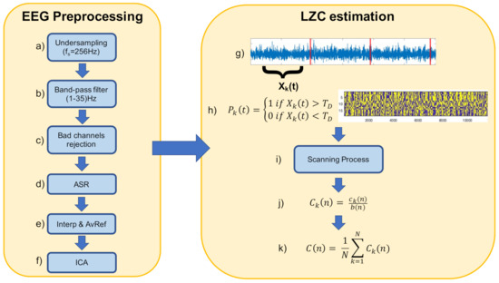
Figure 1.
Schematic illustration of the LZC estimation procedure for one exemplary EEG channel, within a single experimental condition. (a) The EEG data is first undersampled to the sampling frequency of 256 Hz. (b) Then, a band-pass filter in the range (1–35) Hz is applied. (c) Bad channels are identified and rejected, and (d) the Artifact Subspace Reconstruction (ASR) algorithm is applied in order to remove short-time high-amplitude artifacts from the data. Afterwards, (e) bad channels are recovered through interpolation, and the data is referenced to its average. Finally, (f) Independent Component Analysis (ICA) is applied to the data, and components reflecting artifacts activity are removed. (g) Each preprocessed EEG channel is segmented into non-overlapping windows of 39 s length. (h) For each window, the data is transformed into a binary sequence by comparing the time series with its median value. (i) The scanning process is applied to the binary sequence, and (j) the complexity value for the particular window is obtained. Finally, (k) the complexity of each window is averaged, to obtain the complexity of the EEG channel, in a particular experimental condition.
2.6. Tsallis Entropy
In addition to the complexity estimation provided by the LZC, we also performed an entropy analysis to evaluate the randomness and predictability of the EEG time series. We computed the Tsallis entropy (TsEn) of EEG time series according to References [61,62]:
where are the probabilities associated with N possible values of the time series, such that , and q is a parameter measuring the degree of nonextensivity, i.e., , where and are two time series [63]. For each subject and for each experimental condition, we estimated the probability density function of EEG channels through the Sturge’s rule for the choice of the optimal number of bins N in the histograms [64]. We then applied Equation (2) to each time series, using for the nonextensivity parameter [65]. Furthermore, to analyze the contribution of each EEG frequency band, we computed the frequency band TsEn (fTsEn). Specifically, for each subject and for each condition, we band-pass filtered the EEG signal into the , , , and bands, and, for each filtered EEG signal, we computed the TsEn according to the aforementioned procedure.
2.7. Statistical Analysis
We evaluated interactions between groups and conditions (within) by performing two-way ANOVA on TPSD, PSD, LZC, and fLZC, with a significance level of . Since we found no interaction between the two factors, we performed subsequent statistical analysis by considering groups as distinct. We tested for significant differences between conditions (i.e., versus , versus , versus , and versus ) within each group of subjects (i.e., HS, MS, LS). To this aim, we applied a Wilcoxon sign-rank test () to each measure of interest (i.e., TPSD, PSD, LZC, and fLZC). Multiple testing was controlled using the Benjamini-Hochberg False-Discovery-Rate (FDR) procedure for dependent or correlated samples [66]. Then, for each condition, we evaluated between groups differences in TPSD, PSD, LZC, and fLZC with a Kruskal–Wallis test (). We conducted post hoc analysis with a Mann–Whitney test. Multiple testing was controlled with the Tukey–Kramer critical value for independent samples [67].
3. Results
An ANOVA performed on state anxiety scores, between LS, MS, and HS hypnotizability groups was not significant (F(2,31) = 1.77, p = 0.187, = 0.102), indicating that state anxiety did change among hypnotizability groups (HS: M = 32.33, SD = 2.92; LS: M = 37.11, SD = 5.90; MS: M = 35.44, SD = 6.28).
Considering all linear and nonlinear indexes, the results of the ANOVA tests performed for each channel and frequency band did not find any significant interaction between groups and experimental conditions ().
3.1. Power Analysis
Figure 2 depicts the results of the TPSD and PSD analysis within each band for HS, MS, and LS.
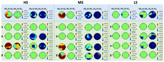
Figure 2.
Within-group analysis of Total Power Spectral Density (TPSD) (blue boxes) and Power Spectral Density (PSD) (green boxes) in the , , , and frequency bands for High-Susceptible (HS) (left), Medium-Susceptible (MS) (center), and Low-Susceptible (LS) (right) subjects, respectively (p < 0.05, False-Discovery-Rate corrected). The red color in the maps corresponds to higher levels of power in the second condition compared to the first, whereas the blue color in the maps corresponds to lower levels of power in the second condition compared to the first.
Between-group analysis of TPSD did not show any significant difference among HS, MS, LS in any experimental condition; thus, the results are not reported. Similarly, we did not find any significant difference between the groups in terms of PSD, for any of the experimental conditions and in any band.
We found similar changes in TPSD for HS and MS. Specifically, we observed lower levels of TPSD under hypnosis, compared to waking rest, in both OE and CE conditions and in almost all scalp regions. Furthermore, we observed higher TPSD during , compared to , in the left frontal, left parietal, and bilateral occipital sites for HS, and in the right frontal and bilateral parietal, temporal, and occipital sites for MS. On the other hand, we did not find any relevant difference between the two hypnotic eye conditions (i.e., versus ), except for few localized changes. For LS, changes in TPSD were slightly different compared to those observed in HS and MS. Specifically, power decreased during , compared to , in the right frontal and left parieto-occipital areas. Furthermore, power also decreased during , compared to , in almost all the scalp regions, and at T3 during versus . Finally, we found no significant differences between OE and CE neither between the two waking rest nor between the two hypnotic conditions.
Concerning the PSD analysis on HS, we found lower levels of -power during hypnosis, compared to rest, in both OE and CE for almost all scalp regions. On the other hand, -power decreased in almost all scalp regions only during . Indeed, during , reduction in TPSD was observed only at Cz (Figure 2). During resting conditions, the observed trends were inverted. In particular, we found an increase of -power in almost all scalp regions during , compared to , and an increase of -power during , compared to , in the frontal, central and occipital sites. Finally, we did not find any significant difference in the and bands. For MS, we observed a decrease in PSD during both OE and CE hypnosis, compared to rest, in the , , and bands. In particular, and power decreased in all the scalp areas during the CE comparisons. Similar to HS, an analogous behavior was observed in the -band for the OE comparison. On the other hand, we found a decrease of -power in temporal and parieto-occipital sites, and a decrease of -power in the right frontal, left temporal, and parieto-occipital sites, respectively, in the OE comparisons. Moreover, we found both an increase of -power in the frontal, temporal, right parietal, and right occipital sites, and an increase of -power in the temporal, parietal, and occipital sites during , compared to . We did not observe any significant difference between the two hypnotic conditions, in any of the considered frequency bands. Furthermore, no significant differences were found in the band for any comparison. For LS, during , we found a decrease of both -power in the frontal, right temporal, central, parietal, and occipital areas, and -power in all the scalp areas, compared to . Moreover, we observed a decrease of power during , compared to , at P3 and T5 for the band and at P3 for the band, respectively. We found no differences between and nor between and .
3.2. Lempel-Ziv Complexity Analysis
For both LZC and fLZC, we found no interaction between groups and conditions.Figure 3 shows the results of LZC and fLZC within-group analysis for HS, MS, and LS. We found an increase of LZC during , compared to , in all the scalp regions, except for C3, Cz, and C4. Furthermore, we observed an increase of complexity in the frontal, temporal, and parietal sites during , compared to in HS. On the other hand, we found lower values of LZC in , compared to , at F3. Similar to HS, MS exhibited higher values of LZC during , compared to , over all the scalp regions, as well as in during compared to , in the right hemisphere and in the left parietal-temporal area (i.e., P3, T5). Furthermore, LZC decreased during , compared to , at F3. On the contrary, we did not find any significant variation of LZC for LS in any of the experimental conditions.
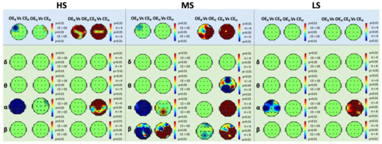
Figure 3.
Within-group analysis of Lempel-Ziv Complexity (LZC) (blue boxes) and frequency-banded LZC (fLZC) (green boxes) in the , , , and frequency bands for High-Susceptible (HS) (left), Medium-Susceptible (MS) (center), and Low-Susceptible (LS) (right) subjects, respectively (, False-Discovery-Rate corrected). The red color in the maps corresponds to higher levels of complexity in the second condition compared to the first, whereas the blue color in the maps corresponds to lower levels of complexity in the second condition compared to the first.
Regarding fLZC, for HS, we observed changes only in the band. Specifically, we observed that, during , complexity decreased compared to in all the scalp regions. Conversely, complexity increased in frontal, central, and occipital areas when comparing with . We did not find any relevant difference between eye conditions during hypnosis nor between hypnosis and rest in OE.
For MS, we found a decrease of complexity during , compared to in all the scalp regions for the band, and for the central, parietal, and occipital regions for the band. Moreover, complexity decreased at Fp2, Pz, and T6 during versus for the band and in the frontal (i.e., Fz), parietal, and occipital areas during versus for the band. Differently, we found an increase of complexity during versus at T3 and Pz for the band, and in the right central, parietal, and occipital sites for the band. Complexity also increased during versus in all the scalp regions for the band, in the right central (i.e., C4), parietal, and occipital sites for the band.
For LS, we observed results similar to HS. Specifically, complexity decreased in the band during , compared to , although limited to the frontal, temporal, and central areas. Moreover, complexity increased during hypnosis, compared to rest, in the CE condition, in almost all the scalp areas.
Figure 4 shows the results of the between-group analysis of LZC. Accordingly, we report the scalp areas for which LZC was different among HS, MS, and LS. In particular, we found differences in complexity between the groups in the left fronto-temporal area and in the area covered by Pz. In Table 1, we report the results of the post-hoc analysis conducted on the significant differences found between the groups. In particular, we observed higher LZC values in MS, compared to HS, in the left fronto-temporal area, whereas, at Pz, we observed higher complexity in LS, compared to HS.
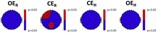
Figure 4.
Between-group analysis of Lempel-Ziv Complexity (LZC) within each experimental condition was conducted with a Kruskal–Wallis test (, corrected with Tukey–Kramer critical value). From left to right: experimental conditions. Red color indicates a significant difference between the groups (i.e., ), whereas blue color indicates no between-group difference (i.e., ).

Table 1.
Post hoc analysis of between-group Lempel-Ziv Complexity (LZC) during Closed-Eye Rest () (median ± median absolute deviation (mad)). Groups consisted of 9 High-Susceptible (HS), 16 Medium-Susceptible (MS), and 9 Low-Susceptible subjects. Rows: electrodes; results are grouped by pairwise comparisons between groups. Significant differences are highlighted in bold. p-values corrected with the Tukey–Kramer critical value.
Results of fLZC between-group analysis are depicted in Figure 5, together with post hoc analysis results resumed in Table 2, Table 3 and Table 4. We found a significant difference at F7 between HS and LS during in the band (Table 2). Furthermore, we observed significant differences during the condition between HS and LS at C3, C4, T5, and Pz, in the band (Table 3). Finally, during the condition, we observed a difference at C3 in the band, although not significant after post hoc analysis (Table 4).
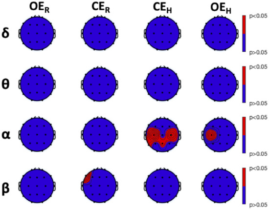
Figure 5.
Between-group analysis of frequency-banded Lempel-Ziv Complexity (fLZC) within each experimental condition was conducted with a Kruskal–Wallis test (, corrected with Tukey–Kramer critical value). Columns: experimental conditions; rows: frequency bands of interest, i.e., , , , and bands. Red color indicates a significant difference between the groups (i.e., ), whereas blue color indicates no between-group difference (i.e., ).
Table 2.
Post hoc analysis of between-group frequency-banded Lempel-Ziv Complexity (fLZC) during Closed-Eye Rest () in the , , , and frequency bands (median ± median absolute deviation (mad)). Groups consisted of 9 High-Susceptible (HS), 16 Medium-Susceptible (MS), and 9 Low-Susceptible subjects. Rows: electrodes; results are grouped by pairwise comparisons between groups. Significant differences are highlighted in bold. p-values corrected with the Tukey–Kramer critical value.
Table 3.
Post hoc analysis of between-group frequency-banded Lempel-Ziv Complexity (fLZC) during Closed-Eye Hypnosis () in the , , , and frequency bands (median ± median absolute deviation (mad)). Groups consisted of 9 High-Susceptible (HS), 16 Medium-Susceptible (MS), and 9 Low-Susceptible subjects. Rows: electrodes; results are grouped by pairwise comparisons between groups. Significant differences are highlighted in bold. p-values corrected with the Tukey–Kramer critical value.
Table 4.
Post hoc analysis of between-group frequency-banded Lempel-Ziv Complexity (fLZC) during Opened-Eye Hypnosis () in the , , , and frequency bands (median ± median absolute deviation (mad)). Groups consisted of 9 High-Susceptible (HS), 16 Medium-Susceptible (MS), and 9 Low-Susceptible subjects. Rows: electrodes; results are grouped by pairwise comparisons between groups. Significant differences are highlighted in bold. p-values corrected with the Tukey–Kramer critical value.
3.3. Tsallis Entropy Analysis
Both TsEn and fTsEn statistical results were not able to significantly discriminate the different experimental conditions within each group. Significant difference were, instead, found between HS and MS groups during the experimental session. Particularly, Figure 6 shows the results of the between-group analysis for TsEn (all red areas refer to HS versus MS significant differences). We observed higher entropy in HS, compared to MS, at F7 during , and in the frontal, temporal, and parietal areas during . Similarly, Figure 7 shows the results of the between-group analysis of fTsEn, carried out for the , , , and bands. We observed higher entropy in HS, compared to MS, during at T7 in the band. Furthermore, we observed higher entropy in HS, compared to MS, during , in the frontal and parieto-occipital areas for the band, in the left frontal, central, and left parieto-temporal areas for the band, in the frontal and parietal areas for the band, and in the frontal and right parietal areas for the band. Notably, we did not find any significant difference between HS and LS nor MS and LS.
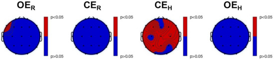
Figure 6.
Post hoc analysis results of the Kruskal–Wallis between-group analysis of Tsallis Entropy (, corrected with the Tukey–Kramer critical value). From left to right: experimental conditions. Red color indicates a higher level of entropy in HS, compared to MS, whereas blue color indicates no significant difference between the two groups.
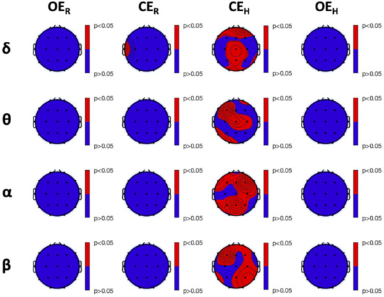
Figure 7.
Post hoc analysis results of the Kruskal–Wallis between-group analysis of frequency-banded Tsallis Entropy (, corrected with the Tukey–Kramer critical value), in the , , , and bands. From left to right: experimental conditions. Red color indicates a higher level of entropy in HS, compared to MS, whereas blue color indicates no significant difference between the two groups.
4. Discussion
In this work, we investigated how hypnotic susceptibility affected EEG correlates in healthy subjects. To this aim, we analyzed EEG recordings from 34 subjects during waking rest and neutral hypnosis, and we investigated the differences in power and complexity measures among HS, MS, and LS. Additionally, for each of waking rest and neutral hypnosis, both OE and CE conditions were considered. More specifically, we evaluated differences in the measures of TPSD, PSD, LZC, and fLZC in four different eye conditions, i.e., , , , . Finally, we performed a between-group analysis to test if there was a statistically significant difference dependent on subjects’ level of hypnotizability.
From the TPSD analysis, we did not observe any significant difference between HS, MS, and LS. Indeed, most of the observed changes between the different experimental conditions were present in all groups. Particularly, a decrease in TPSD during neutral hypnosis compared to waking rest (independently of the eye condition) was manifested in all groups, although such changes were less spread in LS compared to HS and MS. In addition, we did not find any relevant difference between the two eye conditions ( versus ) in hypnosis. This last finding indicates that, during hypnosis, the eye conditions are less relevant than during waking state. This is consistent with previous research showing that MS and HS differ from LS in terms of spontaneous subjective experiences during hypnosis, and some of these experiences are reflected in oscillatory activity (see, e.g., Reference [9]). Likewise, PSD in the different frequency bands reflected similar differences. In particular, we observed that, for both and bands, changes in PSD reflected TPSD results, despite sometimes being more localized. The only relevant difference between HS/MS and LS was, instead, related to the versus . In such comparison, HS/MS participants were reactive to eye modality disclosing a greater power during as compared with , whereas LS did not exhibit any significant variation. These findings as a whole are interesting since they are consistent with the hypothesis that, independently from the eye modality, the attentional focus during hypnosis is on internal stimuli, as it happens for mental imagery [68], rather than external ones [9,69]. However, we cannot exclude that between groups differences were not observed because of the limited number of subjects in the LS and HS groups compared to MS. On the other hand, it may be possible that power features, such as TPSD and PSD, may not be sufficiently specific to distinguish these different groups.
Contrarily to power analysis, complexity results highlighted significant differences between hypnotizability groups for LZC during . In particular, the HS group was significantly different from MS and LS, showing lower values of complexity for left frontal areas, suggesting that the level of hypnotic susceptibility may also have an impact on EEG complexity measures at rest. This finding fits with the idea advanced by References [70,71] of higher cognitive flexibility in HS, as compared to LS, in waking state, and with the higher involvement at the left fronto-limbic level, of the focused attention control system in HS both during the waking-resting phase and the initial stage of the hypnotic induction process [72,73,74]. This result could also be considered in line with [26], in which authors found a higher left hemisphere EEG chaotic activity than in the right one, in distinguishing HS from MS and LS subjects. Additionally, we have also found that HS and LS differed in terms of LZC for Pz. This last result can be explained with original research findings reporting that the parietal region, being part of the focused arousal control system, is more sensitive in HS individuals [75,76].
We also observed between groups differences in fLZC. In particular, since different EEG rhythms may respond differently to neutral hypnosis, we evaluated complexity on filtered EEG in the , , , and bands (i.e., fLZC). Interestingly, differences happened only between HS and LS. We observed that, during , fLZC was lower in HS compared to LS at the F7 electrode in the band. On the other hand, the differences observed during followed a symmetric pattern. In particular, complexity was lower in HS than in LS in the band at C3, C4, Pz, and T5. All these findings can be seen as in line with the model of hypnosis proposed in Reference [74], indicating a shift from a left-hemisphere activation to a hemispheric balance (after hypnotic induction), and then to a right-hemisphere activation to facilitate mental imagery during deep hypnosis.
Within-group analysis showed that LZC was higher for both HS and MS during neutral hypnosis, compared to the waking-resting phase, regardless of eye condition. This is consistent with the results obtained with fLZC. Interestingly, we found these significant differences in the , , and bands, but not in the band. This supports the original results reported in Reference [77], through a reanalysis of the study of Reference [15]. Specifically, authors in Reference [77] found that HS individuals during baseline condition in hypnosis had higher EEG chaotic pointwise dimensions at frontal, temporal, and, to a lessor extent, parietal sites. Based on previous fractal observations reported by Reference [78], authors in Reference [77] interpreted their own dimensionality findings as suggesting that high hypnotic susceptible individuals display underlying brain patterns associated with imagery, whereas low susceptible individuals show patterns consistent with cognitive activity (i.e., mental math). Finally, while LZC showed no significant differences between conditions for LS, fLZC highlighted a significant increase of complexity in the band. Given the above-reported interpretation of LZC findings and given previous observations of enhanced fast- amplitude at rest in the posterior brain of LS [75], we suggest that the significant increase in complexity of the activity could indicate the tendency of LS to deeply relax after the hypnotic induction, rather than experience a mental dimension linked to neutral hypnosis.
Nonlinear measures derived from chaos theory have already been applied to investigate the EEG correlates of hypnosis and hypnotizability. However, the behavior of such measures in the case of short time series or non-stationary data might be not reliable [27]. On the other hand, LZC has the potential to detect complexity even if the time series is generated from a chaotic or a stochastic system because it is a flexible measure that requires no a priori information on the underlying system dynamics [28]. Furthermore, fLZC extend the capabilities of LZC to investigate complexity over frequency bands, which is critical in EEG analysis [60]. Interestingly, within group analysis of complexity measures followed an inverted pattern compared to power measures. Indeed, while complexity increased during hypnosis, power decreased. Moreover, such specular behavior was more accentuated for HS/MS than for LS. Accordingly, we can hypothesize that, for those subjects with higher hypnotic susceptibility, neutral hypnosis induces a mental state associated with higher connectivity. Indeed, the increase in complexity has been associated with more active mental states [28]. Moreover, lower values in power are generally an index of less synchronized global activity, indicating that, during neutral hypnosis, HS and, to a lower extent, MS are experiencing a mental state, such as imagery activity, whereas LS individuals appear to engage in relaxation, such as cognitive activity [77].
LZC-related results have been compared to those obtained by the application of the TsEn and fTsEn. On the one hand, the information provided by the entropy measure was able to significantly discriminate only HS and MS in a single condition, i.e., , for all the frequency bands. On the other hand, both the TsEn and the fTsEn were not able to highlight any difference between experimental conditions, for any of the susceptibility groups, and for any frequency band. This might be related to a low statistical power of the TsEn due to the limited and inhomogeneous number of subjects for each group. However, it is worthwhile to note that the same sample size has been sufficient to obtain the observed significant variations with LZC and fLZC. Furthermore, the Tsallis entropy and LZC indices return different information on nonlinear dynamics related to the concepts of entropy and complexity, since the former can be associated with the level of predictability associated with the time series, while the latter can indicate how chaotic the underlying cortical dynamics are [79]. At the speculation level, this could suggest that modification in the brain’s nonlinear dynamics might be more related to the complexity of the underlying physiological system than to its randomness and predictability properties described by the TsEn index.
In terms of LZC, the HS group was significantly different from MS and LS, showing an asymmetric distribution of complexity with lower complexity at the left frontotemporal area during waking rest with closed eyes, suggesting that the level of hypnotic susceptibility may have an impact on EEG complexity measures also at rest. Further, we observed that fLZC during was lower in HS compared to LS at the F7 electrode in the band, while differences observed during followed an asymmetric pattern with lower complexity in HS than in LS in the band at C3, C4, Pz, and T5. There are experimental pieces of evidence for an inverse relationship between LZC and functional connectivity in non-clinical participants during timing prediction, resting state, and in schizophrenics [80,81,82,83], as well as pieces of evidence for a positive association between fMRI regional neural complexity and network functional connectivity, indicating that a more complex regional neural activity reflects higher functional connectivity [84]. Both the present complexity asymmetry and symmetry findings are new and useful to understand the influence of individual differences in hypnotic susceptibility in brain functioning during neutral hypnosis. However, we suggest that functional connectivity should also be measured to account for the functional integration of the brain [85]. This measure can provide a global view, rather than the local neural activities, for understanding the interactions between distributed brain regions. Comparing observations of both the complexity and functional connectivity under waking rest and neutral hypnosis conditions may provide some new insight for understanding the phenomenon of neutral hypnosis and shed additional light on modeling how the brain works during hypnosis.
Our study comes with limitations. Indeed, our findings are limited to right-handed women and cannot be generalized to men. Moreover, as noted above, findings for individual differences in hypnotic susceptibility may be limited by the small number of participants falling in the HS and LS groups, and a study including a larger number of participants would be a welcome addition to the literature. Finally, we could not conduct EEG localization analyses to detect neural generators reflecting mental state during neutral hypnosis. Future works will exploit connectivity measures and topological data analysis to a detailed characterization of the cortical interactions underlying hypnosis.
5. Conclusions
We found that complexity measures are capable of highlighting peculiarities of subjects with different levels of hypnotic susceptibility compared to standard power analysis. The main results of our work indicate that LZC and fLZC are capable of distinguishing HS, MS, and LS, whereas TPSD and PSD are not. In this view, studying the neural correlates of hypnosis through the use of nonlinear measures may help at characterizing those mental states not resolved with standard measures. In this context, it would be of particular interest to depict the neural sources that give rise to such mental states. Accordingly, we open up to future analyses aiming at characterizing different mental states associated with hypnosis, not only using functional analyses, but also in terms of neural sources involved in such processes.
Author Contributions
Conceptualization, all authors; methodology, G.R., A.L.C., and A.G.; software, G.R. and A.L.C.; validation, G.R., A.L.C., A.G., and V.D.P.; formal analysis, G.R., A.L.C., and A.G.; investigation, V.D.P.; resources, V.D.P.; data curation, V.D.P.; writing—original draft preparation, G.R., A.L.C., V.D.P., and A.G.; writing—review and editing, all authors; visualization, G.R. and A.L.C.; supervision, A.G., E.P.S., and V.D.P.; project administration, A.L.C., A.G., and V.D.P.; funding acquisition, V.D.P. and E.P.S. All authors have read and agreed to the published version of the manuscript.
Funding
This research has received partial funding from the Italian Ministry of Education and Research (MIUR) in the framework of the CrossLab project (Departments of Excellence), and it has been supported in part by a grant from La Sapienza, University of Rome, Italy (project: RG11615502CCDE74), to Prof. Cecilia Guariglia (2016).
Institutional Review Board Statement
The study was conducted according to the guidelines of the Declaration of Helsinki, and approved by the Institutional Review Board of the Department of Psychology of La Sapienza, University of Rome, Rome (RG11615502CCDE74, 2-December-2011).
Informed Consent Statement
Informed consent was obtained from all subjects involved in the study.
Data Availability Statement
Data will be available upon request to the corresponding author.
Acknowledgments
The authors would like to acknowledge the assistance of Paolo Scacchia for hypnotic testing and EEG recordings.
Conflicts of Interest
The authors declare no conflict of interest.
References
- Goodman, M.S.; Kumar, S.; Zomorrodi, R.; Ghazala, Z.; Cheam, A.S.; Barr, M.S.; Daskalakis, Z.J.; Blumberger, D.M.; Fischer, C.; Flint, A.; et al. Theta-gamma coupling and working memory in Alzheimer’s dementia and mild cognitive impairment. Front. Aging Neurosci. 2018, 10, 101. [Google Scholar] [CrossRef] [PubMed]
- Oakley, D.A.; Halligan, P.W. Hypnotic suggestion: Opportunities for cognitive neuroscience. Nat. Rev. Neurosci. 2013, 14, 565–576. [Google Scholar] [CrossRef]
- Landry, M.; Lifshitz, M.; Raz, A. Brain correlates of hypnosis: A systematic review and meta-analytic exploration. Neurosci. Biobehav. Rev. 2017, 81, 75–98. [Google Scholar] [CrossRef] [PubMed]
- Jensen, M.P.; Adachi, T.; Tomé-Pires, C.; Lee, J.; Osman, Z.J.; Miró, J. Mechanisms of Hypnosis: Toward the Development of a Biopsychosocial Model. Int. J. Clin. Exp. Hypn. 2015, 63, 34–75. [Google Scholar] [CrossRef] [PubMed]
- Lynn, S.J.; Kirsch, I. Essentials of Clinical Hypnosis: An Evidence-Based Approach; American Psychological Association: Washington, DC, USA, 2006. [Google Scholar]
- Lipari, S.; Baglio, F.; Griffanti, L.; Mendozzi, L.; Garegnani, M.; Motta, A.; Cecconi, P.; Pugnetti, L. Altered and asymmetric default mode network activity in a “hypnotic virtuoso”: An fMRI and EEG study. Conscious. Cogn. 2012, 21, 393–400. [Google Scholar] [CrossRef] [PubMed]
- Cardeña, E.; Lehmann, D.; Faber, P.L.; Jönsson, P.; Milz, P.; Pascual-Marqui, R.D.; Kochi, K. EEG sLORETA functional imaging during hypnotic arm levitation and voluntary arm lifting. Int. J. Clin. Exp. Hypn. 2012, 60, 31–53. [Google Scholar] [CrossRef]
- Gandhi, B.; Oakley, D.A. Does ‘hypnosis’ by any other name smell as sweet? The efficacy of ‘hypnotic’inductions depends on the label ‘hypnosis’. Conscious. Cogn. 2005, 14, 304–315. [Google Scholar] [CrossRef]
- Cardeña, E.; Jönsson, P.; Terhune, D.B.; Marcusson-Clavertz, D. The neurophenomenology of neutral hypnosis. Cortex 2013, 49, 375–385. [Google Scholar] [CrossRef]
- Kihlstrom, J.F. Neuro-hypnotism: Prospects for hypnosis and neuroscience. Cortex 2013, 49, 365–374. [Google Scholar] [CrossRef]
- Mazzoni, G.; Venneri, A.; McGeown, W.J.; Kirsch, I. Neuroimaging resolution of the altered state hypothesis. Cortex 2013, 49, 400–410. [Google Scholar] [CrossRef]
- Sabourin, M.E.; Cutcomb, S.D.; Crawford, H.J.; Pribram, K. EEG correlates of hypnotic susceptibility and hypnotic trance: Spectral analysis and coherence. Int. J. Psychophysiol. 1990, 10, 125–142. [Google Scholar] [CrossRef]
- Terhune, D.B.; Cardeña, E.; Lindgren, M. Differential frontal-parietal phase synchrony during hypnosis as a function of hypnotic suggestibility. Psychophysiology 2011, 48, 1444–1447. [Google Scholar] [CrossRef] [PubMed]
- De Pascalis, V.; Palumbo, G. EEG alpha asymmetry: Task difficulty and hypnotizability. Percept. Mot. Skills 1986, 62, 139–150. [Google Scholar] [CrossRef]
- Graffin, N.F.; Ray, W.J.; Lundy, R. EEG concomitants of hypnosis and hypnotic susceptibility. J. Abnorm. Psychol. 1995, 104, 123–131. [Google Scholar] [CrossRef]
- Crawford, H.J. Cognitive and psychophysiological correlates of hypnotic responsiveness and hypnosis. In Creative Mastery in Hypnosis and Hypnoanalysis: A Festschrift for Erika Fromm; Lawrence Erlbaum Associates, Inc.: Hillsdale, NJ, USA, 1990; pp. 47–54. [Google Scholar]
- MacLeod-Morgan, C.; Lack, L. Hemispheric specificity: A physiological concomitant of hypnotizability. Psychophysiology 1982, 19, 687–690. [Google Scholar] [CrossRef] [PubMed]
- Freeman, R.; Barabasz, A.; Barabasz, M.; Warner, D. Hypnosis and distraction differ in their effects on cold pressor pain. Am. J. Clin. Hypn. 2000, 43, 137–148. [Google Scholar] [CrossRef] [PubMed]
- Montgomery, D.D.; Dwyer, K.V.; Kelly, S.M. Relationship between QEEG relative power and hypnotic susceptibility. Am. J. Clin. Hypn. 2000, 43, 71–75. [Google Scholar] [CrossRef]
- Schacter, D.L. EEG theta waves and psychological phenomena: A review and analysis. Biol. Psychol. 1977, 5, 47–82. [Google Scholar] [CrossRef]
- Madeo, D.; Castellani, E.; Santarcangelo, E.L.; Mocenni, C. Hypnotic assessment based on the Recurrence Quantification Analysis of EEG recorded in the ordinary state of consciousness. Brain Cogn. 2013, 83, 227–233. [Google Scholar] [CrossRef]
- Chiarucci, R.; Madeo, D.; Loffredo, M.I.; Castellani, E.; Santarcangelo, E.L.; Mocenni, C. Cross-evidence for hypnotic susceptibility through nonlinear measures on EEGs of non-hypnotized subjects. Sci. Rep. 2014, 4, 5610. [Google Scholar] [CrossRef] [PubMed]
- Baghdadi, G.; Nasrabadi, A.M. Comparison of different EEG features in estimation of hypnosis susceptibility level. Comput. Biol. Med. 2012, 42, 590–597. [Google Scholar] [CrossRef]
- Lee, J.S.; Spiegel, D.; Kim, S.B.; Lee, J.H.; Kim, S.I.; Yang, B.H.; Choi, J.H.; Kho, Y.C.; Nam, J.H. Fractal analysis of EEG in hypnosis and its relationship with hypnotizability. Int. J. Clin. Exp. Hypn. 2007, 55, 14–31. [Google Scholar] [CrossRef] [PubMed]
- Yargholi, E.; Nasrabadi, A.M. The impacts of hypnotic susceptibility on chaotic dynamics of EEG signals during standard tasks of Waterloo-Stanford Group Scale. J. Med. Eng. Technol. 2013, 37, 273–281. [Google Scholar] [CrossRef]
- Yargholi, E.; Nasrabadi, A.M. Chaos–chaos transition of left hemisphere EEGs during standard tasks of Waterloo-Stanford Group Scale of hypnotic susceptibility. J. Med. Eng. Technol. 2015, 39, 281–285. [Google Scholar] [CrossRef]
- Stam, C.J. Nonlinear dynamical analysis of EEG and MEG: Review of an emerging field. Clin. Neurophysiol. 2005, 116, 2266–2301. [Google Scholar] [CrossRef] [PubMed]
- Zhang, X.S.; Roy, R.; Jensen, E. EEG complexity as a measure of depth of anesthesia for patients. IEEE Trans. Biomed. Eng. 2001, 48, 1424–1433. [Google Scholar] [CrossRef]
- Ibáñez-Molina, A.J.; Iglesias-Parro, S.; Soriano, M.F.; Aznarte, J.I. Multiscale Lempel-Ziv complexity for EEG measures. Clin. Neurophysiol. 2015, 126, 541–548. [Google Scholar] [CrossRef]
- Tuominen, J.; Kallio, S.; Kaasinen, V.; Railo, H. Segregated brain state during hypnosis. Neurosci. Conscious. 2021, 2021, niab002. [Google Scholar] [CrossRef]
- Lipping, T.; Ferenets, R.; Mortier, E.P.; Struys, M.M.R.F. A new method for evaluating the performance of depth-of-hypnosis indices-the D-value. In Proceedings of the 2007 29th Annual International Conference of the IEEE Engineering in Medicine and Biology Society, Lyon, France, 22–26 August 2007; pp. 6487–6490. [Google Scholar] [CrossRef]
- Bai, Y.; Liang, Z.; Li, X.; Voss, L.J.; Sleigh, J.W. Permutation Lempel–Ziv complexity measure of electroencephalogram in GABAergic anaesthetics. Physiol. Meas. 2015, 36, 2483. [Google Scholar] [CrossRef] [PubMed]
- Hudetz, A.G.; Liu, X.; Pillay, S.; Boly, M.; Tononi, G. Propofol anesthesia reduces Lempel-Ziv complexity of spontaneous brain activity in rats. Neurosci. Lett. 2016, 628, 132–135. [Google Scholar] [CrossRef]
- Hinterberger, T.; Schoner, J.; Halsband, U. Analysis of electrophysiological state patterns and changes during hypnosis induction. Int. J. Clin. Exp. Hypn. 2011, 59, 165–179. [Google Scholar] [CrossRef] [PubMed]
- De Pascalis, V.; Ray, W.J.; Tranquillo, I.; D’Amico, D. EEG activity and heart rate during recall of emotional events in hypnosis: Relationships with hypnotizability and suggestibility. Int. J. Psychophysiol. 1998, 29, 255–275. [Google Scholar] [CrossRef]
- De Pascalis, V. EEG spectral analysis during hypnotic induction, hypnotic dream and age regression. Int. J. Psychophysiol. Off. J. Int. Organ. Psychophysiol. 1993, 15, 153–166. [Google Scholar] [CrossRef]
- Barry, R.J.; Clarke, A.R.; Johnstone, S.J.; Magee, C.A.; Rushby, J.A. EEG differences between eyes-closed and eyes-open resting conditions. Clin. Neurophysiol. 2007, 118, 2765–2773. [Google Scholar] [CrossRef]
- De Pascalis, V.; Scacchia, P. Hypnotizability and placebo analgesia in waking and hypnosis as modulators of auditory startle responses in healthy women: An ERP study. PLoS ONE 2016, 11, e0159135. [Google Scholar] [CrossRef] [PubMed]
- Dumas, R.A. EEG alpha-hypnotizability correlations: A review. Psychophysiology 1977, 14, 431–438. [Google Scholar] [CrossRef] [PubMed]
- Barabasz, A.F. EEG alpha-hypnotizability correlations are not simple covariates of subject self-selection. Biol. Psychol. 1983, 17, 169–172. [Google Scholar] [CrossRef]
- Perlini, A.H.; Spanos, N.P. EEG alpha methodologies and hypnotizability: A critical review. Psychophysiology 1991, 28, 511–530. [Google Scholar] [CrossRef]
- Depascalis, V.; Silveri, A.; Palumbo, G. EEG asymmetry during covert mental activity and its relationship with hypnotizability. Int. J. Clin. Exp. Hypn. 1988, 36, 38–52. [Google Scholar] [CrossRef]
- Cardeña, E.; Kallio, S.; Terhune, D.B.; Buratti, S.; Lööf, A. The effects of translation and sex on hypnotizability testing. Contemp. Hypn. 2007, 24, 154–160. [Google Scholar] [CrossRef]
- Page, R.A.; Green, J.P. An update on age, hypnotic suggestibility, and gender: A brief report. Am. J. Clin. Hypn. 2007, 49, 283–287. [Google Scholar] [CrossRef]
- Költo, A.; Gosi-Greguss, A.C.; Varga, K.; Bányai, É.I. The Influence of Time and Gender on Hungarian Hypnotizability Scores1. Int. J. Clin. Exp. Hypn. 2014, 62, 84–110. [Google Scholar] [CrossRef]
- Oldfield, R.C. The assessment and analysis of handedness: The Edinburgh inventory. Neuropsychologia 1971, 9, 97–113. [Google Scholar] [CrossRef]
- Salmaso, D.; Longoni, A.M. Problems in the assessment of hand preference. Cortex 1985, 21, 533–549. [Google Scholar] [CrossRef]
- Cacioppo, S.; Bianchi-Demicheli, F.; Bischof, P.; DeZiegler, D.; Michel, C.M.; Landis, T. Hemispheric specialization varies with EEG brain resting states and phase of menstrual cycle. PLoS ONE 2013, 8, e63196. [Google Scholar] [CrossRef] [PubMed]
- Huang, Y.; Zhou, R.; Cui, H.; Wu, M.; Wang, Q.; Zhao, Y.; Liu, Y. Variations in resting frontal alpha asymmetry between high-and low-neuroticism females across the menstrual cycle. Psychophysiology 2015, 52, 182–191. [Google Scholar] [CrossRef] [PubMed]
- De Pascalis, V.; Bellusci, A.; Russo, P.M. Italian norms for the Stanford hypnotic susceptibility scale, form C. Int. J. Clin. Exp. Hypn. 2000, 48, 315–323. [Google Scholar] [CrossRef] [PubMed]
- Weitzenhoffer, A.M.; Hilgard, E.R. Stanford Hypnotic Susceptibility Scale, Form C; Consulting Psychologists Press: Palo Alto, CA, USA, 1962; Volume 27. [Google Scholar]
- Spielberger, C.D. State-Trait anxiety inventory. Corsini Encycl. Psychol. 2010, 1-1. [Google Scholar]
- Delorme, A.; Makeig, S. EEGLAB: An open source toolbox for analysis of single-trial EEG dynamics including independent component analysis. J. Neurosci. Methods 2004, 134, 9–21. [Google Scholar] [CrossRef] [PubMed]
- Mullen, T.R.; Kothe, C.A.E.; Chi, Y.M.; Ojeda, A.; Kerth, T.; Makeig, S.; Jung, T.P.; Cauwenberghs, G. Real-Time Neuroimaging and Cognitive Monitoring Using Wearable Dry EEG. IEEE Trans. Bio-Med. Eng. 2015, 62, 2553–2567. [Google Scholar] [CrossRef]
- Chang, C.Y.; Hsu, S.H.; Pion-Tonachini, L.; Jung, T.P. Evaluation of Artifact Subspace Reconstruction for Automatic Artifact Components Removal in Multi-Channel EEG Recordings. IEEE Trans. Biomed. Eng. 2020, 67, 1114–1121. [Google Scholar] [CrossRef]
- Palmer, J.A.; Kreutz-Delgado, K.; Makeig, S. AMICA: An Adaptive Mixture of Independent Component Analyzers with Shared Components; Technical Report; Swartz Center for Computatonal Neursoscience, University of California San Diego: San Diego, CA, USA, 2012. [Google Scholar]
- Lempel, A.; Ziv, J. On the Complexity of Finite Sequences. IEEE Trans. Inf. Theory 1976, 22, 75–81. [Google Scholar] [CrossRef]
- Kaspar, F.; Schuster, H. Easily calculable measure for the complexity of spatiotemporal patterns. Phys. Rev. A 1987, 36, 842. [Google Scholar] [CrossRef] [PubMed]
- Abásolo, D.; Hornero, R.; Gómez, C.; García, M.; López, M. Analysis of EEG background activity in Alzheimer’s disease patients with Lempel–Ziv complexity and central tendency measure. Med. Eng. Phys. 2006, 28, 315–322. [Google Scholar] [CrossRef]
- Al-Nuaimi, A.H.H.; Jammeh, E.; Sun, L.; Ifeachor, E. Complexity measures for quantifying changes in electroencephalogram in Alzheimer’s disease. Complexity 2018, 2018, 8915079. [Google Scholar] [CrossRef]
- Tsallis, C. Possible generalization of Boltzmann-Gibbs statistics. J. Stat. Phys. 1988, 52, 479–487. [Google Scholar] [CrossRef]
- Tsallis, C. Nonextensive statistics: Theoretical, experimental and computational evidences and connections. Braz. J. Phys. 1999, 29, 1–35. [Google Scholar] [CrossRef]
- Gell-Mann, M.; Tsallis, C. Nonextensive Entropy: Interdisciplinary Applications; Oxford University Press: Oxford, UK, 2004. [Google Scholar]
- Scott, D.W. Sturges’ rule. Wiley Interdiscip. Rev. Comput. Stat. 2009, 1, 303–306. [Google Scholar] [CrossRef]
- Zhang, D.; Jia, X.; Ding, H.; Ye, D.; Thakor, N.V. Application of Tsallis entropy to EEG: Quantifying the presence of burst suppression after asphyxial cardiac arrest in rats. IEEE Trans. Biomed. Eng. 2009, 57, 867–874. [Google Scholar] [CrossRef] [PubMed]
- Benjamini, Y.; Yekutieli, D. The control of the false discovery rate in multiple testing under dependency. Ann. Stat. 2001, 29, 1165–1188. [Google Scholar] [CrossRef]
- Peritz, E. Book Reviews: Multiple Comparison Procedures Y. Hochberg and A. C. Tamhane New York: Wiley, 1987. xxii + 450 pp. J. Educ. Stat. 1989, 14, 103–106. [Google Scholar] [CrossRef]
- Klinger, E.; Gregoire, K.C.; Barta, S.G. Physiological correlates of mental activity: Eye movements, alpha, and heart rate during imagining, suppression, concentration, search, and choice. Psychophysiology 1973, 10, 471–477. [Google Scholar] [CrossRef] [PubMed]
- Cooper, N.R.; Burgess, A.P.; Croft, R.J.; Gruzelier, J.H. Investigating evoked and induced electroencephalogram activity in task-related alpha power increases during an internally directed attention task. Neuroreport 2006, 17, 205–208. [Google Scholar] [CrossRef] [PubMed]
- Crawford, H. Cognitive and physiological flexibility: Multiple pathways to hypnotic responsiveness. In Suggestion and Suggestibility; Springer: Berlin/Heidelberg, Germany, 1989; pp. 155–167. [Google Scholar]
- Crawford, H.J.; Gruzelier, J.H. A midstream view of the neuropsychophysiology of hypnosis: Recent research and future directions. In Contemporary Hypnosis Research; Guilford Press: New York, NY, USA, 1992. [Google Scholar]
- Gruzelier, J. The neuropsychology of hypnosis. In Hypnosis: Current Clinical, Experimental and Forensic Practices; Croom Helm: Kent, UK, 1988. [Google Scholar]
- Gruzelier, J. Neuropsychological investigations of hypnosis: Cerebral laterality and beyond. In Hypnosis: Theory, Research and Clinical Practice; Free University Press: Amsterdam, The Netherlands, 1990. [Google Scholar]
- Gruzelier, J. A working model of the neurophysiology of hypnosis: A review of evidence. Contemp. Hypn. 1998, 15, 3–21. [Google Scholar] [CrossRef]
- Sheer, D.E. Sensory and cognitive 40-Hz event-related potentials: Behavioral correlates, brain function, and clinical application. In Brain Dynamics; Springer: Berlin/Heidelberg, Germany, 1989; pp. 339–374. [Google Scholar]
- Pascalis, V.d. Psychophysiological correlates of hypnosis and hypnotic susceptibility. Int. J. Clin. Exp. Hypn. 1999, 47, 117–143. [Google Scholar] [CrossRef]
- Ray, W.J. EEG concomitants of hypnotic susceptibility. Int. J. Clin. Exp. Hypn. 1997, 45, 301–313. [Google Scholar] [CrossRef] [PubMed]
- Lutzenberger, W.; Elbert, T.; Birbaumer, N.; Ray, W.J.; Schupp, H. The scalp distribution of the fractal dimension of the EEG and its variation with mental tasks. Brain Topogr. 1992, 5, 27–34. [Google Scholar] [CrossRef][Green Version]
- Gómez, C.; Hornero, R. Entropy and complexity analyses in Alzheimer’s disease: An MEG study. Open Biomed. Eng. J. 2010, 4, 223. [Google Scholar] [CrossRef]
- Meng, J.; Xu, M.; Zhou, P.; He, F.; Ming, D. EEG complexity and functional connectivity during precise timing prediction. In Proceedings of the 2019 41st Annual International Conference of the IEEE Engineering in Medicine and Biology Society (EMBC), Berlin, Germany, 23–27 July 2019; IEEE: Piscataway, NJ, USA, 2019; pp. 2909–2912. [Google Scholar]
- Mohammadi, Y.; Moradi, M.H. Prediction of Depression Severity Scores Based on Functional Connectivity and Complexity of the EEG Signal. Clin. EEG Neurosci. 2021, 52, 52–60. [Google Scholar] [CrossRef]
- Friston, K.J. Theoretical neurobiology and schizophrenia. Br. Med. Bull. 1996, 52, 644–655. [Google Scholar] [CrossRef]
- Friston, K.J. Dysfunctional connectivity in schizophrenia. World Psychiatry 2002, 1, 66. [Google Scholar] [PubMed]
- Wang, D.J.; Jann, K.; Fan, C.; Qiao, Y.; Zang, Y.F.; Lu, H.; Yang, Y. Neurophysiological basis of multi-scale entropy of brain complexity and its relationship with functional connectivity. Front. Neurosci. 2018, 12, 352. [Google Scholar] [CrossRef] [PubMed]
- Baccalá, L.A.; Sameshima, K. Partial directed coherence: A new concept in neural structure determination. Biol. Cybern. 2001, 84, 463–474. [Google Scholar] [CrossRef] [PubMed]
Publisher’s Note: MDPI stays neutral with regard to jurisdictional claims in published maps and institutional affiliations. |
© 2021 by the authors. Licensee MDPI, Basel, Switzerland. This article is an open access article distributed under the terms and conditions of the Creative Commons Attribution (CC BY) license (https://creativecommons.org/licenses/by/4.0/).