Bayesian Inference for the Parameters of Kumaraswamy Distribution via Ranked Set Sampling

Abstract

In this paper, we address the estimation of the parameters for a two-parameter Kumaraswamy distribution by using the maximum likelihood and Bayesian methods based on simple random sampling, ranked set sampling, and maximum ranked set sampling with unequal samples. The Bayes loss functions used are symmetric and asymmetric. The Metropolis-Hastings-within-Gibbs algorithm was employed to calculate the Bayes point estimates and credible intervals. We illustrate a simulation experiment to compare the implications of the proposed point estimators in sense of bias, estimated risk, and relative efficiency as well as evaluate the interval estimators in terms of average confidence interval length and coverage percentage. Finally, a real-life example and remarks are presented.

1. Introduction

The Kumaraswamy distribution was proposed for double-bounded random processes by [1]. The cumulative distribution function (CDF) and the corresponding probability density function (PDF) can be expressed as

$$\begin{array}{c}\hfill F(x;\theta ,\beta )=1-{(1-x^{\theta })}^{\beta },0<x<1;\theta ,\beta >0\end{array}$$

(1)

and:

$$\begin{array}{c}\hfill f(x;\theta ,\beta )=\theta \beta x^{\theta -1}{\left(1-x^{\theta }\right)}^{\beta -1},0<x<1;\theta ,\beta >0\end{array}$$

(2)

respectively.

For simplicity, we denote Kumaraswamy distribution with two positive parameters $\theta$ and $\beta$ as $K(\theta ,\beta )$. Based on varying values of $\theta$ and $\beta$, there are similar shape properties between Kumaraswamy distribution and Beta distribution. However, the former is superior to the latter in some respects: there are not any special functions involved in $K(\theta ,\beta )$ and its quantile function; the generation of random variables is simple, as L-moments and moments of order statistics for $K(\theta ,\beta )$ have simple formulars (see [2]). For the PDF of $K(\theta ,\beta )$, as shown on the left of Figure 1, when $\theta >1$ and $\beta >1$, it is unimodal; when $\theta >1$ and $\beta \le 1$, it is increasing; when $\theta \le 1$ and $\beta >1$, it is decreasing; when $\theta <1$ and $\beta <1$, it is uniantimodal; when $\theta =\beta =1$, it is constant. The CDF of $K(\theta ,\beta )$ (the plot is presented on the right of Figure 1) has an explicit expression, while the CDF of the Beta distribution appears in an integral form. Therefore, Kumaraswamy distribution is considered as a substitutive model for Beta distribution in practical terms. For instance, Kumaraswamy distribution has an outstanding fitting effect on daily rainfall, individual heights, unemployment numbers, and ball bearing revolutions (see [3,4,5,6]).

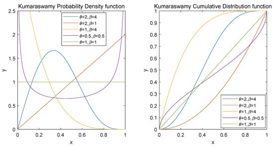
Figure 1. PDF and CDF of $K(\theta ,\beta )$.

Recently, Kumaraswamy distribution has drawn much academic attention and concern. The authors in Ref. [7] obtained the estimators of parameters for Kumaraswamy distribution based on the progressive type-II censoring data using Bayesian and non-Bayesian methods; the authors in Ref. [8] studied the estimations of parameters for this distribution under hybrid censoring; the authors in Ref. [9] ulteriorly discussed the estimations of the stress–strength parameters based on an incorporation of progressive type II and hybrid censoring schemes. Then, the authors in Ref. [10] continued to focus on this distribution under hybrid progressive type I censored samples. The authors in Ref. [11] discussed the estimations of parameters in Kumaraswamy distribution under the generalized progressive hybrid censored samples. On the basis of the Kumaraswamy distribution, a range of new distributions were proposed, such as the Kumaraswamy Birnbaum–Saunders distribution due to [12]), generalized inverted Kumaraswamy distribution due to [13], and transmuted Kumaraswamy distribution due to [14].

Ranked set sampling (RSS), first introduced by [15], is considered to be a more effective method than simple random sampling (SRS) in estimating the mean values of a distribution (see [16]). It is appropriate to employ RSS in many fields where sampling schemes cost a lot of human strength and money. It has a widespread application in the domains of the environment, biology, engineering applications, and agriculture (see [17,18,19,20]). Recently, the authors in Ref. [21] proposed a new sampling design known as the maximum ranked set sampling procedure with unequal samples (MRSSU).

The difficulties overcome in this paper are that (a) it is difficult to obtain the solutions of the equations of maximum likelihood estimation to tackle Big Data problems [22]. Hence, we adopted the Newton–Raphson iterative algorithm to derive the approximate and numerical roots; (b) since it is difficult to express the integrals for Bayes estimates in closed forms [23], we chose the Metropolis-Hastings-within-Gibbs algorithm to obtain the estimates [24,25,26,27,28].

The organization of this paper is summarized as follows. In Section 2, Section 3 and Section 4, we consider point and interval estimates for Kumaraswamy distribution based on three sampling schemes, namely SRS, RSS, and MRSSU, and two estimation methods of maximum likelihood estimation and Bayes estimation. Section 5 compares the performance of proposed estimators and Section 6 presents an illustrative example. This paper concludes with some comments in Section 7.

2. Estimations of the Parameters Using SRS

2.1. Maximum Likelihood Estimations Based on SRS

Considering that $X=(X_1,X_2,\cdots ,X_s)$ is an SRS scheme of size s from $K(\theta ,\beta )$ and the likelihood function is given by

$$\begin{array}{c}\hfill L_1(\theta ,\beta )={\theta }^s{\beta }^s\prod _{i=1}^s{x}_i^{\theta -1}{(1-x_i^{\theta })}^{\beta -1},\end{array}$$

where $\tilde{x}=(x_1,x_2,\cdots ,x_s)$ is the observed sample of X. The corresponding log-likelihood function is:

$$\begin{array}{c}\hfill l_1(\theta ,\beta )=sln\theta +sln\beta +(\theta -1)\sum _{i=1}^{s}ln{x}_i+(\beta -1)\sum _{i=1}^{s}ln(1-x_i^{\theta }).\end{array}$$

(3)

Calculate the first derivatives of (3) about $\theta$, $\beta$ and equate them to zero. The maximum likelihood estimates (MLEs) of $\theta$ and $\beta$ can be earned by solving follow equations:

$$\begin{array}{ccc}\hfill \frac{\partial l_1(\theta ,\beta )}{\partial \theta }& =& \frac{s}{\theta }+\sum _{i=1}^{s}ln{x}_i-(\beta -1)\sum _{i=1}^s\frac{x_i^{\theta }ln{x}_i}{1-x_i^{\theta }}=0,\hfill \end{array}$$

(4)

$$\begin{array}{ccc}\hfill \frac{\partial l_1(\theta ,\beta )}{\partial \beta }& =& \frac{s}{\beta }+\sum _{i=1}^{s}ln(1-x_i^{\theta })=0.\hfill \end{array}$$

(5)

We obtain the MLE of $\beta$ and denote it as

$$\begin{array}{c}\hfill {\widehat{\beta }}_{MLE}=-\frac{s}{{\sum }_{i=1}^{s}ln(1-x_i^{\theta })}\end{array}$$

(6)

According to the formula in (6), ${\widehat{\beta }}_{MLE}$ exists and is unique for fixed $\theta$. Substituting the (6) into (3), the profile log-likelihood function of $\theta$ can be expressed as

$$\begin{array}{c}\hfill P\left(\theta \right)=sln\theta +sln\left(-\frac{s}{{\sum }_{i=1}^{s}ln(1-x_i^{\theta })}\right)+(\theta -1)\sum _{i=1}^{s}ln{x}_i-\sum _{i=1}^{s}ln(1-x_i^{\theta })-s.\end{array}$$

(7)

${\widehat{\theta }}_{MLE}$ is defined to the MLE of $\theta$, which can be obtained by maximizing (7). Since it is difficult to determine the explicit solutions of $\theta$ and $\beta$, the Newton–Raphson iterative algorithm is adopted to obtain MLEs.

Theorem 1.

${\widehat{\theta }}_{MLE}$ exists and is unique.

Proof of Theorem 1.

Calculate the first and second derivatives of (7) about $\theta$:

$$\begin{array}{ccc}\hfill P{}^{\prime }\left(\theta \right)& =& \frac{s}{\theta }\left[1+\frac{D_1}{D_2}+D_3\right],\hfill \end{array}$$

(8)

$$\begin{array}{ccc}\hfill P^{{}^{″}}\left(\theta \right)& =& -\frac{s}{{\theta }^2}\left[E_1+\frac{E_2}{{[{\sum }_{i=1}^{s}ln(1-x_i^{\theta })]}^2}\right],\hfill \end{array}$$

(9)

where:

$$\begin{array}{ccc}\hfill D_1& =& \sum _{i=1}^s\frac{x_i^{\theta }ln{x}_i^{\theta }}{1-x_i^{\theta }},D_2=\sum _{i=1}^{s}ln(1-x_i^{\theta }),D_3=\frac{1}{s}\sum _{i=1}^s\frac{ln{x}_i^{\theta }}{1-x_i^{\theta }},\hfill \\ \hfill E_1& =& 1-\frac{1}{s}\sum _{i=1}^s\frac{x_i^{\theta }{(ln{x}_i^{\theta })}^2}{{(1-x_i^{\theta })}^2},\hfill \\ \hfill E_2& =& \left(\sum _{i=1}^s\frac{x_i^{\theta }{(ln{x}_i^{\theta })}^2}{{(1-x_i^{\theta })}^2}\right)\left(\sum _{i=1}^s-ln(1-x_i^{\theta })\right)-{\left(\sum _{i=1}^s\frac{x_i^{\theta }ln{x}_i^{\theta }}{1-x_i^{\theta }}\right)}^2.\hfill \end{array}$$

From (8), ${lim}_{\theta \to 0^{+}}\frac{s}{\theta }=+\infty$, ${lim}_{\theta \to 0^{+}}s\frac{D_1}{D_2}>0$ and ${lim}_{\theta \to 0^{+}}{D}_3=-\frac{1}{s}<1$, it means that ${lim}_{\theta \to 0^{+}}[1+\frac{D_1}{D_2}+D_3]>0$. Therefore, when $\theta \to 0^{+}$, $P^{{}^{\prime }}\left(\theta \right)\to +\infty$. Meanwhile, ${lim}_{\theta \to +\infty }\frac{s}{\theta }=0$, ${lim}_{\theta \to +\infty }\frac{s}{\theta }\frac{D_1}{D_2}={\sum }_{i=1}^{s}ln{x}_i$ and ${lim}_{\theta \to +\infty }\frac{s}{\theta }{D}_3={\sum }_{i=1}^{s}ln{x}_i$. Therefore, when $\theta \to +\infty$,$P^{{}^{″}}\left(\theta \right)=2{\sum }_{i=1}^{s}ln{x}_i<0$. According to Cauchy–Schwarz inequality, since:

$$\begin{array}{ccc}\hfill \left(\sum _{i=1}^s\frac{x_i^{\theta }{(ln{x}_i^{\theta })}^2}{{(1-x_i^{\theta })}^2}\right)\left(\sum _{i=1}^s-ln(1-x_i^{\theta })\right)& \ge & {\left(\sum _{i=1}^s\frac{x_i^{\frac{\theta }{2}}ln{x}_i^{\theta }}{1-x_i^{\theta }}\sqrt{-ln(1-x_i^{\theta })}\right)}^2\hfill \\ & >& {\left(\sum _{i=1}^s\frac{x_i^{\theta }ln{x}_i^{\theta }}{1-x_i^{\theta }}\right)}^2\hfill \end{array}$$

then $E_2>0$. With $E_1>0$, consequently, $P^{{}^{″}}\left(\theta \right)<0$ and (7) is concave. The result is proven. □

We then consider the confidence intervals (CIs) under the SRS scheme based on maximum likelihood estimation. The second derivatives of (3) can be expressed as

$$\begin{array}{ccc}\hfill \frac{{\partial }^2{l}_1(\theta ,\beta )}{\partial {\theta }^2}& =& -\frac{s}{{\theta }^2}-\sum _{i=1}^s(\beta -1)\frac{x_i^{\theta }{(ln{x}_i)}^2}{{(1-x_i^{\theta })}^2},\hfill \\ \hfill \frac{{\partial }^2{l}_1(\theta ,\beta )}{\partial {\beta }^2}& =& -\frac{s}{{\beta }^2},\hfill \\ \hfill \frac{{\partial }^2{l}_1(\theta ,\beta )}{\partial \theta \partial \beta }& =& \frac{{\partial }^2{l}_1(\theta ,\beta )}{\partial \beta \partial \theta }=-\sum _{i=1}^s\frac{x_i^{\theta }ln{x}_i}{1-x_i^{\theta }}.\hfill \end{array}$$

Denote $\eta =(\theta ,\beta )$, and the expected Fisher information matrix $I\left(\eta \right)$ is given by

$$\begin{array}{c}\hfill I\left(\eta \right)=\left[\begin{array}{cc}{I}_{11}& I_{12}\\ I_{21}& I_{22}\end{array}\right]=\mathrm{E}\left[\begin{array}{cc}-\frac{{\partial }^2{l}_1\left(\theta ,\beta \right)}{\partial {\theta }^2}& -\frac{{\partial }^2{l}_1\left(\theta ,\beta \right)}{\partial \theta \partial \beta }\\ -\frac{{\partial }^2{l}_1\left(\theta ,\beta \right)}{\partial \beta \partial \theta }& -\frac{{\partial }^2{l}_1\left(\theta ,\beta \right)}{\partial {\beta }^2}\end{array}\right].\end{array}$$

Here:

$$\begin{array}{ccc}\hfill I_{11}& =& \frac{s\beta }{\theta }{\int }_0^1{x}^{\theta -1}{(1-x^{\theta })}^{\beta -1}\mathrm{d}x+s\theta ({\beta }^2-\beta ){\int }_0^1{x}^{2\theta -1}{(1-x^{\theta })}^{\beta -3}{(lnx)}^2\mathrm{d}x,\hfill \\ \hfill I_{22}& =& \frac{s\beta }{\theta }{\int }_0^1{x}^{\theta -1}{(1-x^{\theta })}^{\beta -1}\mathrm{d}x,\hfill \\ \hfill I_{12}& =& I_{22}=s\theta \beta {\int }_0^1{x}^{2\theta -1}{(1-x^{\theta })}^{\beta -2}lnx\mathrm{d}x.\hfill \end{array}$$

Let ${\widehat{\eta }}_{MLE.SRS}$ be the MLEs of $\eta$ based on SRS. The inverse matrix of $I\left(\widehat{\eta }\right)$ is the approximate variance–covariance matrix of MLEs with:

$$\begin{array}{c}\hfill I^{-1}\left(\widehat{\eta }\right)=\left[\begin{array}{cc}\mathrm{Var}\left({\widehat{\theta }}_{MLE.SRS}\right)& \mathrm{Cov}({\widehat{\theta }}_{MLE.SRS},{\widehat{\beta }}_{MLE.SRS})\\ \mathrm{Cov}({\widehat{\beta }}_{MLE.SRS},{\widehat{\theta }}_{MLE.SRS})& \mathrm{Var}\left({\widehat{\beta }}_{MLE.SRS}\right)\end{array}\right].\end{array}$$

(10)

The asymptotic distribution of ${\widehat{\eta }}_{MLE.SRS}$ is $({\widehat{\eta }}_{MLE.SRS}-\eta )\to N(0,I^{-1}\left({\widehat{\eta }}_{MLE.SRS}\right))$. Thus, we derive the two-sided $100(1-\tau )\%$ approximate confidence intervals (ACIs) for $\theta$ and $\beta$.

Theorem 2.

The two-sided $100(1-\tau )\%$ ACIs for θ, β based on SRS are:

$$\begin{array}{c}\hfill \left[max\left(0,{\widehat{\theta }}_{MLE.SRS}-u_{\tau /2}\sqrt{\mathrm{Var}\left({\widehat{\theta }}_{MLE.SRS}\right)}\right),{\widehat{\theta }}_{MLE.SRS}+u_{\tau /2}\sqrt{\mathrm{Var}\left({\widehat{\theta }}_{MLE.SRS}\right)}\right]\end{array}$$

and:

$$\begin{array}{c}\hfill \left[max\left(0,{\widehat{\beta }}_{MLE.SRS}-u_{\tau /2}\sqrt{\mathrm{Var}\left({\widehat{\beta }}_{MLE.SRS}\right)}\right),{\widehat{\beta }}_{MLE.SRS}+u_{\tau /2}\sqrt{\mathrm{Var}\left({\widehat{\beta }}_{MLE.SRS}\right)}\right]\end{array}$$

respectively.

Here, $u_{\tau }$ is the $(1-\tau )$th quantile of $N(0,1)$, the standard normal distribution. Since the lower bound for the CI will possibly be less than zero and $\theta$, $\beta$ are greater than zero, we set the lower bound to be the larger value of the computed lower bound and zero.

2.2. Bayes Estimations Based on SRS

In this section, we focus on Bayesian inference of $\theta$ and $\beta$ based on SRS, and obtain Bayesian estimates (BEs) and credible intervals (CrIs). Let us consider the following independent gamma priors:

$$\begin{array}{ccc}\hfill {\pi }_1\left(\theta \right)& =& \frac{{\mu }_1^{v_1}}{\mathsf{\Gamma }\left(v_1\right)}{\theta }^{v_1-1}{e}^{-{\mu }_1\theta },\hfill \end{array}$$

(11)

$$\begin{array}{ccc}\hfill {\pi }_2\left(\beta \right)& =& \frac{{\mu }_2^{v_2}}{\mathsf{\Gamma }\left(v_2\right)}{\beta }^{v_2-1}{e}^{-{\mu }_2\beta }.\hfill \end{array}$$

(12)

The joint posterior distribution of $(\theta ,\beta )$ can be expressed as

$$\begin{array}{c}\hfill {\mathsf{\Pi }}_1(\theta ,\beta |\tilde{x})=\frac{{\theta }^{s+v_1-1}{\beta }^{s+v_2-1}}{C_1}{e}^{-{\mu }_1\theta -{\mu }_2\beta }\prod _{i=1}^s{x}_i^{\theta -1}{(1-x_i^{\theta })}^{\beta -1},\end{array}$$

(13)

where:

$$\begin{array}{c}\hfill C_1={\int }_0^{\infty }{\int }_0^{\infty }{\theta }^{s+v_1-1}{\beta }^{s+v_2-1}{e}^{-{\mu }_1\theta -{\mu }_2\beta }\prod _{i=1}^s{x}_i^{\theta -1}{(1-x_i^{\theta })}^{\beta -1}\mathrm{d}\theta \mathrm{d}\beta .\end{array}$$

The conditional posterior densities of $\theta$ and $\beta$ are written as

$$\begin{array}{c}\hfill {\mathsf{\Pi }}_1\left(\theta \right|\beta ,\tilde{x})\propto {\theta }^{s+v_1-1}{e}^{-{\mu }_1\theta }\prod _{i=1}^s{x}_i^{\theta -1}{(1-x_i^{\theta })}^{\beta -1}\end{array}$$

and:

$$\begin{array}{c}\hfill {\mathsf{\Pi }}_1\left(\beta \right|\theta ,\tilde{x})\propto {\beta }^{s+v_2-1}{e}^{-{\mu }_2\beta }\prod _{i=1}^s{(1-x_i^{\theta })}^{\beta -1}.\end{array}$$

Generally, Bayes point estimators are acquired by minimizing the loss function. Here, we consider two typical loss functions. The first one is symmetric, which is the square error (SE) loss function. Let $\widehat{d}$ be the estimator of d, and the definition of SE loss function and Bayes estimators are given by

$$\begin{array}{c}\hfill L_{SE}(d,\widehat{d})={(d-\widehat{d})}^2\end{array}$$

and:

$$\begin{array}{c}\hfill {\widehat{d}}_{BE.SE}={\mathrm{E}}_d\left(d\right|\tilde{x}).\end{array}$$

Symmetric functions assign equal weight to both overestimation and underestimation, so there emerge many asymmetric functions. The second is the general entropy (GE) loss function, which is an asymmetric function proposed by [29] defined as

$$\begin{array}{c}\hfill L_{GE}(d,\widehat{d})\propto {\left(\frac{\widehat{d}}{d}\right)}^k-kln\left(\frac{\widehat{d}}{d}\right)-1,k\ne 0.\end{array}$$

The corresponding Bayes estimator is:

$$\begin{array}{c}\hfill {\widehat{d}}_{BE.GE}={\left[{\mathrm{E}}_d\left(d^{-k}\right|\tilde{x})\right]}^{-\frac{1}{k}}.\end{array}$$

Here, the positive errors $(\widehat{d}>d)$ make more mistakes than the negative errors when $k>0$, and vice versa when $k<0$.

Based on SE and GE loss functions, Bayes point estimators of $\theta$ can be gained as

$$\begin{array}{c}\hfill {\widehat{\theta }}_{BE.SE.SRS}={\int }_0^{\infty }{\int }_0^{\infty }\frac{{\theta }^{n+v_1}{\beta }^{n+v_2-1}}{C_1}{e}^{-{\mu }_1\theta -{\mu }_2\beta }\prod _{i=1}^n{x}_i^{\theta -1}{(1-x_i^{\theta })}^{\beta -1}\mathrm{d}\theta \mathrm{d}\beta \end{array}$$

and:

$$\begin{array}{c}\hfill {\widehat{\theta }}_{BE.GE.SRS}={\left[{\int }_0^{\infty }{\int }_0^{\infty }\frac{{\theta }^{n+v_1-1-k}{\beta }^{n+v_2-1}}{C_1}{e}^{-{\mu }_1\theta -{\mu }_2\beta }\prod _{i=1}^n{x}_i^{\theta -1}{(1-x_i^{\theta })}^{\beta -1}\mathrm{d}\theta \mathrm{d}\beta \right]}^{-\frac{1}{k}}\end{array}$$

provided that the expectations exist, while the Bayes estimator of $\beta$ is able to be obtained in a similar way. It is easily observed that while using the above integrals, it is difficult to gain the explicit solutions. Therefore, we employed the MHG algorithm to generate samples from the posterior density distribution (13) and computed the approximated BEs and the $100(1-\gamma )\%$ symmetric CrIs. More information about this algorithm can be found in [30].

The logarithmic calculations in the 5th and 11th steps of Algorithm 1 are for the purpose of narrowing down the value to facilitate the calculation and preventing the generation of infinity in the process of program operation.

We can obtain the approximated Bayes point estimates of $\theta$ and $\beta$ under the SE and GE loss functions as

$$\begin{array}{c}\hfill {\widehat{\theta }}_{BE.SE.SRS}^{\ast }=\frac{1}{M-H}\sum _{t=H+1}^M{\theta }^{\left(t\right)}\end{array}$$

and:

$$\begin{array}{c}\hfill {\widehat{\theta }}_{BE.GE.SRS}^{\ast }={\left[\frac{1}{M-H}\sum _{t=H+1}^M{\left({\theta }^{\left(t\right)}\right)}^{-k}\right]}^{-\frac{1}{k}}\end{array}$$

where H is a burn-in period (which refers to the iteration times required before the stationary distribution is reached). ${\widehat{\beta }}_{BE.SE.SRS}^{\ast }$ and ${\widehat{\beta }}_{BE.GE.SRS}^{\ast }$ can be acquired by a similar way.

Order ${\theta }^{(H+1)},\cdots ,{\theta }^{\left(M\right)}$ and ${\beta }^{(H+1)},\cdots ,{\beta }^{\left(M\right)}$ as ${\theta }_1,\cdots ,{\theta }_{M-H}$ and ${\beta }_1,\cdots ,{\beta }_{M-H}$. Then, the $100(1-\gamma )\%$ symmetric Bayes CrIs of $\theta$ and $\beta$ are acquired by

$$\begin{array}{c}\hfill \left[{\theta }_{\frac{\gamma }{2}(M-H)},{\theta }_{(1-\frac{\gamma }{2})(M-H)}\right]\end{array}$$

and:

$$\begin{array}{c}\hfill \left[{\beta }_{\frac{\gamma }{2}(M-H)},{\beta }_{(1-\frac{\gamma }{2})(M-H)}\right]\end{array}$$

respectively.

Algorithm 1 The Metropolis-Hastings-within-Gibbs algorithm

Input:M: total number of iterations. Output:${\theta }^{\left(1\right)},\cdots$, ${\theta }^{\left(M\right)}$ and ${\beta }^{\left(1\right)},\cdots ,{\beta }^{\left(M\right)}$.   Initial ${\theta }^{\left(0\right)}={\widehat{\theta }}_{MLE}$, ${\beta }^{\left(0\right)}={\widehat{\beta }}_{MLE}$ and $T=1$.   while $T\le M$ do     Generate $\tilde{\theta }$ and $\tilde{\beta }$ from $N({\theta }^{(T-1)},{\sigma }_1)$ and $N({\beta }^{(T-1)},{\sigma }_2)$, two normal distributions, where ${\sigma }_1$ and ${\sigma }_2$ are diagonal elements of the variance–covariance matrix.     Generate $u_1$ from the Uniform distribution $U(0,1)$.     $R_1=log{\mathsf{\Pi }}_1\left(\tilde{\theta }\right|{\beta }^{\left(T\right)},\tilde{x})+logq\left({\theta }^{(T-1)}\right|\tilde{\theta })-log{\mathsf{\Pi }}_1\left({\theta }^{(T-1)}\right|{\beta }^{\left(T\right)},\tilde{x})-logq\left(\tilde{\theta }\right|{\theta }^{(T-1)})$     if $log{u}_2<min\left\{R_1,0\right\}$ then         ${\theta }^{\left(T\right)}=\tilde{\theta }$. Here, $q\left(x\right|y)$ is the probability density of $N(y,{\sigma }_1)$.     else         ${\theta }^{\left(T\right)}={\theta }^{(T-1)}$     Generate $u_2$ from the Uniform distribution $U(0,1)$.     $R_2=log{\mathsf{\Pi }}_1\left(\tilde{\beta }\right|{\theta }^{\left(T\right)},\tilde{x})+logq\left({\beta }^{(T-1)}\right|\tilde{\beta })-log{\mathsf{\Pi }}_1\left({\beta }^{(T-1)}\right|{\theta }^{\left(T\right)},\tilde{x})-logq\left(\tilde{\beta }\right|{\beta }^{(T-1)})$     if $log{u}_2<min\left\{R_2,0\right\}$ then         ${\beta }^{\left(T\right)}=\tilde{\beta }$. Here, $q\left(x\right|y)$ is the probability density of $N(y,{\sigma }_2)$.     else         ${\beta }^{\left(T\right)}={\beta }^{(T-1)}$         $T=T+1$

3. Estimations of the Parameters Using RSS

3.1. Maximum Likelihood Estimations Based on RSS

The RSS scheme aims to sample and observe the data by using the ranking mechanism. First, we draw m random sample sets of size m from $K(\theta ,\beta )$ and sort each dataset from the smallest to the largest, meaning that:

$$\begin{array}{c}\hfill \left(\begin{array}{cccc}{\mathit{X}}_{\mathbf{1}(\mathbf{1}:\mathit{m})}^{\left(i\right)}& X_{1(2:m)}^{\left(i\right)}& \cdots & X_{1(m:m)}^{\left(i\right)}\\ X_{2(1:m)}^{\left(i\right)}& {\mathit{X}}_{\mathbf{2}(\mathbf{2}:\mathit{m})}^{\left(i\right)}& \cdots & X_{2(m:m)}^{\left(i\right)}\\ ⋮& ⋮& \ddots & ⋮\\ X_{m(1:m)}^{\left(i\right)}& X_{m(2:m)}^{\left(i\right)}& \cdots & {\mathit{X}}_{\mathit{m}(\mathit{m}:\mathit{m})}^{\left(i\right)}\end{array}\right).\end{array}$$

Here, $X_{j(p:m)}^{\left(i\right)}$ means p-th ranked units, j-th set, and i-th cycle ($i=1,2,\cdots ,n;j=1,2,\cdots ,m$). Then, the j-th ordered unit from the j-th set ($X_{j(j:m)}^{\left(i\right)}$) is chosen for practical quantification. After n cycle of above process, we end up with a complete RSS scheme of size $mn$ expressed as

$$\begin{array}{c}\hfill \left(\begin{array}{cccc}{X}_{1(1:m)}^{\left(1\right)}& X_{2(2:m)}^{\left(1\right)}& \cdots & X_{m(m:m)}^{\left(1\right)}\\ X_{1(1:m)}^{\left(2\right)}& X_{2(2:m)}^{\left(2\right)}& \cdots & X_{m(m:m)}^{\left(2\right)}\\ ⋮& ⋮& \ddots & ⋮\\ X_{1(1:m)}^{\left(n\right)}& X_{2(2:m)}^{\left(n\right)}& \cdots & X_{m(m:m)}^{\left(n\right)}\end{array}\right),\end{array}$$

where m is the set size and n is the number of cycles.

To simplify the notations, we use $X_{ij}$ to denote $X_{j(j:m)}^{\left(i\right)}$. Let $X^{\ast }=(X_{11},X_{12},\cdots ,X_{nm})$. The likelihood function is given by

$$\begin{array}{c}\hfill L_2(\theta ,\beta )={\theta }^{mn}{\beta }^{mn}\prod _{i=1}^n\prod _{j=1}^{m}j\left(\genfrac{}{}{0pt}{}{m}{j}\right)x_{ij}^{\theta -1}{(1-x_{ij}^{\theta })}^{(1+m-j)\beta -1}{[1-{(1-x_{ij}^{\theta })}^{\beta }]}^{j-1},\end{array}$$

where $x^{\ast }=(x_{11},x_{12},\cdots ,x_{nm})$ is the observed sample of $X^{\ast }$, and the log-likelihood function is:

$$\begin{array}{cc}\hfill l_2(\theta ,\beta )=& mnln\theta +mnln\beta +\sum _{i=1}^n\sum _{j=1}^{m}ln\left[j\left(\genfrac{}{}{0pt}{}{m}{j}\right)\right]+(\theta -1)\sum _{i=1}^n\sum _{j=1}^{m}ln{x}_{ij}\hfill \\ & +\sum _{i=1}^n\sum _{j=1}^m\left[(1+m-j)\beta -1\right]ln(1-x_{ij}^{\theta })+\sum _{i=1}^n\sum _{j=1}^m(j-1)ln\left[1-{(1-x_{ij}^{\theta })}^{\beta }\right].\hfill \end{array}$$

(14)

Calculate the first derivatives of (14) about $\theta$, $\beta$ and equate them to zero. The MLEs of $\theta$, $\beta$ can be earned by solving the follow system of equations:

$$\begin{array}{cc}\hfill \frac{\partial l_2(\theta ,\beta )}{\partial \theta }=& \frac{mn}{\theta }+\sum _{i=1}^n\sum _{j=1}^{m}ln{x}_{ij}-\sum _{i=1}^n\sum _{j=1}^m[(1+m-j)\beta -1]\frac{x_{ij}^{\theta }ln{x}_{ij}}{1-x_{ij}^{\theta }}\hfill \end{array}$$

$$\begin{array}{c}\hfill +\sum _{i=1}^n\sum _{j=1}^m(j-1)\frac{\beta x_{ij}^{\theta }{(1-x_{ij}^{\theta })}^{\beta -1}ln{x}_{ij}}{1-{(1-x_{ij}^{\theta })}^{\beta }},\end{array}$$

(15)

$$\begin{array}{cc}\hfill \frac{\partial l_2(\theta ,\beta )}{\partial \beta }=& \frac{mn}{\beta }+\sum _{i=1}^n\sum _{j=1}^m(1+m-j)ln(1-x_{ij}^{\theta })-\sum _{i=1}^n\sum _{j=1}^m(j-1)\frac{{(1-x_{ij}^{\theta })}^{\beta }ln(1-x_{ij}^{\theta })}{1-{(1-x_{ij}^{\theta })}^{\beta }}.\hfill \end{array}$$

(16)

The second derivatives of (14) are expressed as

$$\begin{array}{cc}\hfill \frac{{\partial }^2{l}_2(\theta ,\beta )}{\partial {\theta }^2}=& -\frac{mn}{{\theta }^2}-\sum _{i=1}^n\sum _{j=1}^m[(1+m-j)\beta -1]\frac{x_{ij}^{2\theta }{(ln{x}_{ij})}^2}{{(1-x_{ij}^{\theta })}^2}\hfill \\ \hfill & -\sum _{i=1}^n\sum _{j=1}^m[(1+m-j)\beta -1]\frac{x_{ij}^{\theta }{(ln{x}_{ij})}^2}{1-x_{ij}^{\theta }}\hfill \\ \hfill & -\sum _{i=1}^n\sum _{j=1}^m(j-1)\frac{{\beta }^2{x}_{ij}^{2\theta }{(1-x_{ij}^{\theta })}^{-2+2\beta }{(ln{x}_{ij})}^2}{{[1-{(1-x_{ij}^{\theta })}^{\beta }]}^2}\hfill \\ \hfill & +\sum _{i=1}^n\sum _{j=1}^m(j-1)\frac{\beta x_{ij}^{\theta }{(1-x_{ij}^{\theta })}^{-1+\beta }{(ln{x}_{ij})}^2}{1-{(1-x_{ij}^{\theta })}^{\beta }}\hfill \\ \hfill & -\sum _{i=1}^n\sum _{j=1}^m(j-1)\frac{({\beta }^2-\beta )x_{ij}^{2\theta }{(1-x_{ij}^{\theta })}^{-2+\beta }{(ln{x}_{ij})}^2}{1-{(1-x_{ij}^{\theta })}^{\beta }},\hfill \\ \hfill \frac{{\partial }^2{l}_2(\theta ,\beta )}{\partial {\beta }^2}=& -\frac{mn}{{\beta }^2}-\sum _{i=1}^n\sum _{j=1}^m(j-1)\frac{{(1-x_{ij}^{\theta })}^{2\beta }{[ln(1-x_{ij}^{\theta })]}^2}{{[1-{(1-x_{ij}^{\theta })}^{\beta }]}^2}\hfill \\ \hfill & -\sum _{i=1}^n\sum _{j=1}^m(j-1)\frac{{(1-x_{ij}^{\theta })}^{\beta }{[ln(1-x_{ij}^{\theta })]}^2}{1-{(1-x_{ij}^{\theta })}^{\beta }},\hfill \\ \hfill \frac{{\partial }^2{l}_2(\theta ,\beta )}{\partial \theta \partial \beta }=& \frac{{\partial }^2{l}_2(\theta ,\beta )}{\partial \beta \partial \theta }\hfill \\ \hfill =& -\sum _{i=1}^n\sum _{j=1}^m(1+m-j)\frac{x_{ij}^{\theta }ln{x}_{ij}}{1-x_{ij}^{\theta }}\hfill \\ \hfill & +\sum _{i=1}^n\sum _{j=1}^m(j-1)\frac{\beta x_{ij}^{\theta }{(1-x_{ij}^{\theta })}^{-1+2\beta }ln{x}_{ij}ln(1-x_{ij}^{\theta })}{{[1-{(1-x_{ij}^{\theta })}^{\beta }]}^2}\hfill \\ \hfill & +\sum _{i=1}^n\sum _{j=1}^m(j-1)\frac{\left[1+\beta ln(1-x_{ij}^{\theta })\right]x_{ij}^{\theta }{(1-x_{ij}^{\theta })}^{-1+\beta }ln{x}_{ij}}{1-{(1-x_{ij}^{\theta })}^{\beta }}.\hfill \end{array}$$

We can derive the expected Fisher information matrix $I^{\ast }\left(\eta \right)$, where:

$$\begin{array}{c}\hfill I^{\ast }\left(\eta \right)=\mathrm{E}\left[\begin{array}{cc}-\frac{{\partial }^2{l}_2\left(\theta ,\beta \right)}{\partial {\theta }^2}& -\frac{{\partial }^2{l}_2\left(\theta ,\beta \right)}{\partial \theta \partial \beta }\\ -\frac{{\partial }^2{l}_2\left(\theta ,\beta \right)}{\partial \beta \partial \theta }& -\frac{{\partial }^2{l}_2\left(\theta ,\beta \right)}{\partial {\beta }^2}\end{array}\right].\end{array}$$

Because the integral form of matrix $I^{\ast }\left(\eta \right)$ is difficult to calculate, the observed Fisher information matrix $J^{\ast }\left(\eta \right)$ is used to replace matrix $I^{\ast }\left(\eta \right)$, where:

$$\begin{array}{c}\hfill J^{\ast }\left(\eta \right)=\left[\begin{array}{cc}-\frac{{\partial }^2{l}_2\left(\theta ,\beta \right)}{\partial {\theta }^2}& -\frac{{\partial }^2{l}_2\left(\theta ,\beta \right)}{\partial \theta \partial \beta }\\ -\frac{{\partial }^2{l}_2\left(\theta ,\beta \right)}{\partial \beta \partial \theta }& -\frac{{\partial }^2{l}_2\left(\theta ,\beta \right)}{\partial {\beta }^2}\end{array}\right].\end{array}$$

Let ${\widehat{\eta }}_{MLE.RSS}$ be the MLEs of $\eta$. The inverse matrix of $J^{\ast }\left(\widehat{\eta }\right)$ is the approximate variance–covariance matrix of MLEs with:

$$\begin{array}{c}\hfill {\left(J^{\ast }\left(\widehat{\eta }\right)\right)}^{-1}=\left[\begin{array}{cc}\mathrm{Var}\left({\widehat{\theta }}_{MLE.RSS}\right)& \mathrm{Cov}({\widehat{\theta }}_{MLE.RSS},{\widehat{\beta }}_{MLE.RSS})\\ \mathrm{Cov}({\widehat{\beta }}_{MLE.RSS},{\widehat{\theta }}_{MLE.RSS})& \mathrm{Var}\left({\widehat{\beta }}_{MLE.RSS}\right)\end{array}\right].\end{array}$$

(17)

Theorem 3.

The two-sided $100(1-\tau )\%$ ACIs for θ and β based on RSS are given by

$$\begin{array}{c}\hfill \left[max\left(0,{\widehat{\theta }}_{MLE.RSS}-u_{\tau /2}\sqrt{Var\left({\widehat{\theta }}_{MLE.RSS}\right)}\right),{\widehat{\theta }}_{MLE.RSS}+u_{\tau /2}\sqrt{Var\left({\widehat{\theta }}_{MLE.RSS}\right)}\right]\end{array}$$

and:

$$\begin{array}{c}\hfill \left[max\left(0,{\widehat{\beta }}_{MLE.RSS}-u_{\tau /2}\sqrt{Var\left({\widehat{\beta }}_{MLE.RSS}\right)}\right),{\widehat{\beta }}_{MLE.RSS}+u_{\tau /2}\sqrt{Var\left({\widehat{\beta }}_{MLE.RSS}\right)}\right]\end{array}$$

respectively.

3.2. Bayes Estimations Based on RSS

We still use independent gamma priors (11) and (12). The joint posterior distribution of $(\theta ,\beta )$ is:

$$\begin{array}{c}\hfill {\mathsf{\Pi }}_2(\theta ,\beta |x^{\ast })=\frac{{\theta }^{mn+v_1-1}{\beta }^{mn+v_2-1}}{C_2}{e}^{-{\mu }_1\theta -{\mu }_2\beta }\prod _{i=1}^n\prod _{j=1}^m{x}_{ij}^{\theta -1}{(1-x_{ij}^{\theta })}^{(1+m-j)\beta -1}{\left[1-{(1-x_{ij}^{\theta })}^{\beta }\right]}^{j-1},\end{array}$$

(18)

$$\begin{array}{c}\hfill C_2={\int }_0^{\infty }{\int }_0^{\infty }{\theta }^{mn+v_1-1}{\beta }^{mn+v_2-1}{e}^{-{\mu }_1\theta -{\mu }_2\beta }\prod _{i=1}^n\prod _{j=1}^m{x}_{ij}^{\theta -1}{(1-x_{ij}^{\theta })}^{(1+m-j)\beta -1}{\left[1-{(1-x_{ij}^{\theta })}^{\beta }\right]}^{j-1}.\end{array}$$

The conditional posterior densities of $\theta$, $\beta$ are given by

$$\begin{array}{c}\hfill {\mathsf{\Pi }}_2\left(\theta \right|\beta ,x^{\ast })\propto {\theta }^{mn+v_1-1}{e}^{-{\mu }_1\theta }\prod _{i=1}^n\prod _{j=1}^m{x}_{ij}^{\theta -1}{(1-x_{ij}^{\theta })}^{(1+m-j)\beta -1}{\left[1-{(1-x_{ij}^{\theta })}^{\beta }\right]}^{j-1}\end{array}$$

and:

$$\begin{array}{c}\hfill {\mathsf{\Pi }}_2\left(\beta \right|\theta ,x^{\ast })\propto {\beta }^{mn+v_2-1}{e}^{{\mu }_2\beta }\prod _{i=1}^n\prod _{j=1}^m{(1-x_{ij}^{\theta })}^{(1+m-j)\beta -1}{\left[1-{(1-x_{ij}^{\theta })}^{\beta }\right]}^{j-1}.\end{array}$$

The Algorithm 1 mentioned in Section 2 was employed to generate a large number of samples from the posterior distribution (18). Then, Bayes point estimators of $\theta$ under SE and GE loss functions are given by

$$\begin{array}{c}\hfill {\widehat{\theta }}_{BE.SE.RSS}^{\ast }=\frac{1}{M-H}\sum _{t=H+1}^M{\theta }^{\left(t\right)}\end{array}$$

and:

$$\begin{array}{c}\hfill {\widehat{\theta }}_{BE.GE.RSS}^{\ast }={\left[\frac{1}{M-H}\sum _{t=H+1}^M{\left({\theta }^{\left(t\right)}\right)}^{-k}\right]}^{-\frac{1}{k}},\end{array}$$

Order the sample ${\theta }^{(H+1)},{\theta }^{(H+2)},\cdots ,{\theta }^{\left(M\right)}$ as ${\theta }_1,{\theta }_2,\cdots ,{\theta }_{M-H}$. Then, symmetric Bayes CrIs of $\theta$ is given by

$$\begin{array}{c}\hfill \left[{\theta }_{\frac{\gamma }{2}(M-H)},{\theta }_{(1-\frac{\gamma }{2})(M-H)}\right].\end{array}$$

Similarly, we can derive the Bayes point estimators and symmetric Bayes CrI for $\beta$.

4. Estimations of the Parameters Using MRSSU

4.1. Maximum Likelihood Estimations Based on MRSSU

First, we select m random sample sets from the population, where the j-th sample set possesses j units $(j=1,2,\cdots ,m)$ and sort the units in each dataset from smallest to largest, meaning that:

$$\begin{array}{c}\hfill \left(\begin{array}{c}{\mathit{X}}_{\mathbf{1}(\mathbf{1}:\mathbf{1})}^{\left(i\right)}\\ X_{2(1:2)}^{\left(i\right)}& {\mathit{X}}_{\mathbf{2}(\mathbf{2}:\mathbf{2})}^{\left(i\right)}\\ ⋮& ⋮& \ddots \\ X_{m(1:m)}^{\left(i\right)}& X_{m(2:m)}^{\left(i\right)}& \cdots & {\mathit{X}}_{\mathit{m}(\mathit{m}:\mathit{m})}^{\left(i\right)}\end{array}\right).\end{array}$$

Here, $X_{j(p:m)}^{\left(i\right)}$ means p-th ranked units, the j-th set which contains j units and i-th cycle ($i=1,2,\cdots ,n;j=1,2,\cdots ,m$). In each circle, the total number of units of samples we draw is $\frac{(1+m)m}{2}$.

Then, the maximum element in each sample set ($X_{j(j:m)}^{\left(i\right)}$) is chosen for practical quantification. After n iterations of the above process, we end up with a complete MRSSU of size $mn$ expressed as

$$\begin{array}{c}\hfill \left(\begin{array}{cccc}{X}_{1(1:1)}^{\left(1\right)}& X_{2(2:2)}^{\left(1\right)}& \cdots & X_{m(m:m)}^{\left(1\right)}\\ X_{1(1:1)}^{\left(2\right)}& X_{2(2:2)}^{\left(2\right)}& \cdots & X_{m(m:m)}^{\left(2\right)}\\ ⋮& ⋮& \ddots & ⋮\\ X_{1(1:1)}^{\left(n\right)}& X_{2(2:2)}^{\left(n\right)}& \cdots & X_{m(m:m)}^{\left(n\right)}\end{array}\right),\end{array}$$

where m is the set size and n is the number of cycles.

To simplify the notations, we used $Y_{ij}$ to denote $X_{j(j:j)}^{\left(i\right)}$. Let $Y=(Y_{11},Y_{12},\cdots ,Y_{nm})$. The corresponding likelihood function is:

$$\begin{array}{c}\hfill L_3(\theta ,\beta )={\theta }^{mn}{\beta }^{mn}\prod _{i=1}^n\prod _{j=1}^{m}j{y}_{ij}^{\theta -1}{(1-y_{ij}^{\theta })}^{\beta -1}{[1-{(1-y_{ij}^{\theta })}^{\beta }]}^{j-1},\end{array}$$

where $\tilde{y}=(y_{11},y_{12},\cdots ,y_{nm})$ is the observation of Y, and the log-likelihood function is:

$$\begin{array}{cc}\hfill l_3(\theta ,\beta )=& -mnln\theta +mnln\beta +\sum _{i=1}^n\sum _{j=1}^{m}lnj+(\theta -1)\sum _{i=1}^n\sum _{j=1}^{m}ln{y}_{ij}\hfill \\ & +\left(\beta -1\right)\sum _{i=1}^n\sum _{j=1}^{m}ln(1-x_{ij}^{\theta })+\sum _{i=1}^n\sum _{j=1}^m(j-1)ln\left[1-{(1-x_{ij}^{\theta })}^{\beta }\right].\hfill \end{array}$$

(19)

Calculate the first derivatives of (19) about $\theta$, $\beta$ and equate them to zero. By solving the follow equations:

$$\begin{array}{cc}\hfill \frac{\partial l_3(\theta ,\beta )}{\partial \theta }=& \frac{mn}{\theta }+\sum _{i=1}^n\sum _{j=1}^{m}ln{y}_{ij}-(\beta -1)\sum _{i=1}^n\sum _{j=1}^m\frac{y_{ij}^{\theta }ln{y}_{ij}}{1-y_{ij}^{\theta }}\hfill \end{array}$$

$$\begin{array}{c}\hfill +\sum _{i=1}^n\sum _{j=1}^m(j-1)\frac{\beta y_{ij}^{\theta }{(1-y_{ij}^{\theta })}^{\beta -1}ln{y}_{ij}}{1-{(1-y_{ij}^{\theta })}^{\beta }},\end{array}$$

(20)

$$\begin{array}{cc}\hfill \frac{\partial l_3(\theta ,\beta )}{\partial \beta }=& \frac{mn}{\beta }+\sum _{i=1}^n\sum _{j=1}^{m}ln(1-y_{ij}^{\theta })-\sum _{i=1}^n\sum _{j=1}^m(j-1)\frac{{(1-y_{ij}^{\theta })}^{\beta }ln(1-y_{ij}^{\theta })}{1-{(1-y_{ij}^{\theta })}^{\beta }},\hfill \end{array}$$

(21)

the MLEs of $\theta$, $\beta$ can be earned. The second derivatives of (19) are expressed as

$$\begin{array}{cc}\hfill \frac{{\partial }^2{l}_3(\theta ,\beta )}{\partial {\theta }^2}=& \frac{mn}{{\theta }^2}-(\beta -1)\sum _{i=1}^n\sum _{j=1}^m\frac{y_{ij}^{2\theta }{(ln{y}_{ij})}^2}{{(1-y_{ij}^{\theta })}^2}-(\beta -1)\sum _{i=1}^n\sum _{j=1}^m\frac{y_{ij}^{\theta }{(ln{y}_{ij})}^2}{1-y_{ij}^{\theta }}\hfill \\ & -\sum _{i=1}^n\sum _{j=1}^m(j-1)\frac{{\beta }^2{y}_{ij}^{2\theta }{(1-y_{ij}^{\theta })}^{-2+2\beta }{(ln{y}_{ij})}^2}{{[1-{(1-y_{ij}^{\theta })}^{\beta }]}^2}\hfill \\ \hfill & +\sum _{i=1}^n\sum _{j=1}^m(j-1)\frac{\beta y_{ij}^{\theta }{(1-y_{ij}^{\theta })}^{-1+\beta }{(ln{y}_{ij})}^2}{1-{(1-y_{ij}^{\theta })}^{\beta }}\hfill \\ \hfill & -\sum _{i=1}^n\sum _{j=1}^m(j-1)\frac{({\beta }^2-\beta )y_{ij}^{2\theta }{(1-y_{ij}^{\theta })}^{-2+\beta }{(ln{y}_{ij})}^2}{1-{(1-y_{ij}^{\theta })}^{\beta }},\hfill \\ \hfill \frac{{\partial }^2{l}_3(\theta ,\beta )}{\partial {\beta }^2}=& -\frac{mn}{{\beta }^2}-\sum _{i=1}^n\sum _{j=1}^m(j-1)\frac{{(1-y_{ij}^{\theta })}^{2\beta }{[ln(1-y_{ij}^{\theta })]}^2}{{[1-{(1-y_{ij}^{\theta })}^{\beta }]}^2}\hfill \\ \hfill & -\sum _{i=1}^n\sum _{j=1}^m(j-1)\frac{{(1-y_{ij}^{\theta })}^{\beta }{[ln(1-y_{ij}^{\theta })]}^2}{1-{(1-y_{ij}^{\theta })}^{\beta }},\hfill \\ \hfill \frac{{\partial }^2{l}_2(\theta ,\beta )}{\partial \theta \partial \beta }=& \frac{{\partial }^2{l}_2(\theta ,\beta )}{\partial \beta \partial \theta }\hfill \\ \hfill =& -\sum _{i=1}^n\sum _{j=1}^m\frac{y_{ij}^{\theta }ln{y}_{ij}}{1-y_{ij}^{\theta }}+\sum _{i=1}^n\sum _{j=1}^m(j-1)\frac{\beta y_{ij}^{\theta }{(1-y_{ij}^{\theta })}^{-1+2\beta }ln(1-y_{ij}^{\theta })}{{[1-{(1-y_{ij}^{\theta })}^{\beta }]}^{2}ln{y}_{ij}}\hfill \\ \hfill & +\sum _{i=1}^n\sum _{j=1}^m(j-1)\frac{\left[1+\beta ln(1-y_{ij}^{\theta })\right]y_{ij}^{\theta }{(1-y_{ij}^{\theta })}^{-1+\beta }ln{y}_{ij}}{1-{(1-x_{ij}^{\theta })}^{\beta }}.\hfill \end{array}$$

Thus, we derive expected Fisher information matrix $I^{\ast \ast }\left(\eta \right)$, where:

$$\begin{array}{c}\hfill I^{\ast \ast }\left(\eta \right)=\mathrm{E}\left[\begin{array}{cc}-\frac{{\partial }^2{l}_3\left(\theta ,\beta \right)}{\partial {\theta }^2}& -\frac{{\partial }^2{l}_3\left(\theta ,\beta \right)}{\partial \theta \partial \beta }\\ -\frac{{\partial }^2{l}_3\left(\theta ,\beta \right)}{\partial \beta \partial \theta }& -\frac{{\partial }^2{l}_3\left(\theta ,\beta \right)}{\partial {\beta }^2}\end{array}\right].\end{array}$$

We adopt the observed Fisher information matrix $J^{\ast \ast }\left(\eta \right)$ to replace matrix $I^{\ast \ast }\left(\eta \right)$, where:

$$\begin{array}{c}\hfill J^{\ast \ast }\left(\eta \right)=\left[\begin{array}{cc}-\frac{{\partial }^2{l}_3\left(\theta ,\beta \right)}{\partial {\theta }^2}& -\frac{{\partial }^2{l}_3\left(\theta ,\beta \right)}{\partial \theta \partial \beta }\\ -\frac{{\partial }^2{l}_3\left(\theta ,\beta \right)}{\partial \beta \partial \theta }& -\frac{{\partial }^2{l}_3\left(\theta ,\beta \right)}{\partial {\beta }^2}\end{array}\right].\end{array}$$

Let ${\widehat{\eta }}_{MLE.MRSSU}$ be the MLEs of $\eta$. The inverse matrix of $J^{\ast \ast }\left(\widehat{\eta }\right)$ is the approximate variance–covariance matrix of MLEs with:

$$\begin{array}{c}\hfill {\left(J^{\ast \ast }\left(\widehat{\eta }\right)\right)}^{-1}=\left[\begin{array}{cc}\mathrm{Var}\left({\widehat{\theta }}_{MLE.MRSSU}\right)& \mathrm{Cov}({\widehat{\theta }}_{MLE.MRSSU},{\widehat{\beta }}_{MLE.MRSSU})\\ \mathrm{Cov}({\widehat{\beta }}_{MLE.MRSSU},{\widehat{\theta }}_{MLE.MRSSU})& \mathrm{Var}\left({\widehat{\beta }}_{MLE.MRSSU}\right)\end{array}\right].\end{array}$$

(22)

Theorem 4.

The two-sided $100(1-\tau )\%$ ACIs for θ, β based MRSSU are given by

$$\begin{array}{c}\hfill \left[max\left(0,{\widehat{\theta }}_{MLE.MRSSU}-u_{\tau /2}\sqrt{\mathrm{Var}\left({\widehat{\theta }}_{MLE.MRSSU}\right)}\right),{\widehat{\theta }}_{MLE.MRSSU}+u_{\tau /2}\sqrt{\mathrm{Var}\left({\widehat{\theta }}_{MLE.MRSSU}\right)}\right],\end{array}$$

$$\begin{array}{c}\hfill \left[max\left(0,{\widehat{\beta }}_{MLE.MRSSU}-u_{\tau /2}\sqrt{\mathrm{Var}\left({\widehat{\beta }}_{MLE.MRSSU}\right)}\right),{\widehat{\beta }}_{MLE.MRSSU}+u_{\tau /2}\sqrt{\mathrm{Var}\left({\widehat{\beta }}_{MLE.MRSSU}\right)}\right],\end{array}$$

respectively.

4.2. Bayes Estimations Based on MRSSU

We use the same independent gamma priors (11) and (12). The joint posterior distribution of $(\theta ,\beta )$ is:

$$\begin{array}{c}\hfill {\mathsf{\Pi }}_3(\theta ,\beta |\tilde{y})=\frac{{\theta }^{n+v_1-1}{\beta }^{n+v_2-1}}{C_3}{e}^{-{\mu }_1\theta -{\mu }_2\beta }\prod _{i=1}^n\prod _{j=1}^m{y}_{ij}^{\theta -1}{(1-y_{ij}^{\theta })}^{\beta -1}{\left[1-{(1-y_{ij}^{\theta })}^{\beta }\right]}^{j-1},\end{array}$$

(23)

where:

$$\begin{array}{c}\hfill C_3={\int }_0^{\infty }{\int }_0^{\infty }{\theta }^{mn+v_1-1}{\beta }^{mn+v_2-1}{e}^{-{\mu }_1\theta -{\mu }_2\beta }\prod _{i=1}^n\prod _{j=1}^m{y}_{ij}^{\theta -1}{(1-y_{ij}^{\theta })}^{\beta -1}{\left[1-{(1-y_{ij}^{\theta })}^{\beta }\right]}^{j-1}.\end{array}$$

The conditional posterior densities of $\theta$, $\beta$ are denoted by

$$\begin{array}{c}\hfill {\mathsf{\Pi }}_3\left(\theta \right|\beta ,\tilde{y})\propto {\theta }^{mn+v_1-1}{e}^{-{\mu }_1\theta }\prod _{i=1}^n\prod _{j=1}^m{y}_{ij}^{\theta -1}{(1-y_{ij}^{\theta })}^{\beta -1}{\left[1-{(1-y_{ij}^{\theta })}^{\beta }\right]}^{j-1}\end{array}$$

and:

$$\begin{array}{c}\hfill {\mathsf{\Pi }}_3\left(\beta \right|\theta ,\tilde{y})\propto {\beta }^{mn+v_2-1}{e}^{{\mu }_2\beta }\prod _{i=1}^n\prod _{j=1}^m{(1-y_{ij}^{\theta })}^{\beta -1}{\left[1-{(1-y_{ij}^{\theta })}^{\beta }\right]}^{j-1}.\end{array}$$

The Algorithm 1 is used to generate a large number of samples from the posterior distribution (23). Then, Bayes point estimators of $\theta$ under SE and GE loss functions, are expressed as

$$\begin{array}{c}\hfill {\widehat{\theta }}_{BE.SE.MRSSU}^{\ast }=\frac{1}{M-H}\sum _{t=H+1}^M{\theta }^{\left(t\right)}\end{array}$$

and:

$$\begin{array}{c}\hfill {\widehat{\theta }}_{BE.GE.MRSSU}^{\ast }={\left[\frac{1}{M-H}\sum _{t=H+1}^M{\left({\theta }^{\left(t\right)}\right)}^{-k}\right]}^{-\frac{1}{k}}.\end{array}$$

Order the sample ${\theta }^{(H+1)},{\theta }^{(H+2)},\cdots ,{\theta }^{\left(M\right)}$ as ${\theta }_1,{\theta }_2,\cdots ,{\theta }_{M-H}$. Symmetric Bayes CrI of $\theta$ is given by

$$\begin{array}{c}\hfill \left[{\theta }_{\frac{\gamma }{2}(M-H)},{\theta }_{(1-\frac{\gamma }{2})(M-H)}\right].\end{array}$$

Similarly, we can derive the Bayes point estimators and symmetric Bayes CrI for $\beta$.

5. Simulation Result

In this section, we intend to carry out comparisons of the SRS, RSS, and MRSSU schemes under different hyperparameter values and sample sizes, by comparing the numerical performance of point estimates and interval estimates. We evaluate bias and estimated risks (ERs) based on SE and GE loss functions by the following formulas:

$$\begin{array}{cc}\hfill Bias\left(\widehat{\theta }\right)& =\frac{1}{N}\sum _{t=1}^N\left({\widehat{\theta }}_t-\theta \right),\hfill \\ \hfill E{R}_{SE}\left(\widehat{\theta }\right)& =\frac{1}{N}\sum _{t=1}^N{\left({\widehat{\theta }}_t-\theta \right)}^2,\hfill \\ \hfill E{R}_{GE}\left(\widehat{\theta }\right)& =\frac{1}{N}\sum _{t=1}^N\left[{\left(\frac{{\widehat{\theta }}_t}{\theta }\right)}^k-kln\left(\frac{{\widehat{\theta }}_t}{\theta }\right)-1\right].\hfill \end{array}$$

Here, N denotes the iteration number of the simulation while ${\widehat{\theta }}_t$ means the estimate obtained in the t-th iteration. As for the three sampling methods, namely RSR, RSS and MRSSU, we can draw the samples, respectively, from $K(\theta ,\beta )$ through Algorithms 2–4:

Algorithm 2 The random number generator for $K(\theta ,\beta )$ based on SRS

Input:$\theta$, $\beta$ and s. Output:$x_1,x_2,\cdots ,x_s$.   initial $i^{\ast }=1$.   while $i^{\ast }\le s$ do     Generate $u\sim U(0,1)$.     $x_{i^{\ast }}={(1-u^{\frac{1}{\beta }})}^{\frac{1}{\theta }}$     $i^{\ast }=i^{\ast }+1$

Algorithm 3 The random number generator for $K(\theta ,\beta )$ based on RSS

Input:$\theta$, $\beta$, n and m. Output:$x_{11},x_{12},\cdots ,x_{nm}$.   initial $i=1$ and $j=1$.   while $i\le n$ do     while $j\le m$ do         Use Algorithm 2 (input $s=M$) to generate $x_1,x_2,\cdots ,x_m$.         Rank $x_1,x_2,\cdots ,x_m$ from smallest to largest to get $x_{\left(1\right)},x_{\left(2\right)},\cdots ,x_{\left(m\right)}$.         $x_{ij}=x_{\left(j\right)}$.         $j=j+1$.     $i=i+1$.

Algorithm 4 The random number generator for $K(\theta ,\beta )$ based on MRSSU

Input:$\theta$, $\beta$, n and m. Output:$x_{11},x_{12},\cdots ,x_{nm}$.   initial $i=1$ and $j=1$.   while $i\le n$ do     while $j\le m$ do         Use Algorithm 2 (input $s=j$) to generate $x_1,x_2,\cdots ,x_j$.         Rank $x_1,x_2,\cdots ,x_j$ from smallest to largest to get $x_{\left(1\right)},x_{\left(2\right)},\cdots ,x_{\left(j\right)}$.         $x_{ij}=x_{\left(j\right)}$.         $j=j+1$.     $i=i+1$.

In addition, based on different sampling schemes, we evaluate the relative efficiency (RE) values based on SE and GE loss functions which are given by

$$\begin{array}{cc}\hfill R{E}_{SE1}& =\frac{E{R}_{SE}\left({\widehat{\theta }}_{RSS}\right)}{E{R}_{SE}\left({\widehat{\theta }}_{SRS}\right)},R{E}_{SE2}=\frac{E{R}_{SE}\left({\widehat{\theta }}_{RSS}\right)}{E{R}_{SE}\left({\widehat{\theta }}_{MRSSU}\right)},R{E}_{SE3}=\frac{E{R}_{SE}\left({\widehat{\theta }}_{MRSSU}\right)}{E{R}_{SE}\left({\widehat{\theta }}_{SRS}\right)},\hfill \\ \hfill R{E}_{GE1}& =\frac{E{R}_{GE}\left({\widehat{\theta }}_{RSS}\right)}{E{R}_{GE}\left({\widehat{\theta }}_{SRS}\right)},R{E}_{GE2}=\frac{E{R}_{GE}\left({\widehat{\theta }}_{RSS}\right)}{E{R}_{GE}\left({\widehat{\theta }}_{MRSSU}\right)},R{E}_{GE3}=\frac{E{R}_{GE}\left({\widehat{\theta }}_{MRSSU}\right)}{E{R}_{GE}\left({\widehat{\theta }}_{SRS}\right)}.\hfill \end{array}$$

Here, ${\widehat{\theta }}_{SRS},{\widehat{\theta }}_{RSS},{\widehat{\theta }}_{MRSSU}$ are the corresponding estimates of $\theta$ based on different sample methods. Obviously, if $E{R}_i<1(i=1,2,\dots ,6)$, then we know the estimate of $\theta$ in the numerator outperforms the estimate of $\theta$ in the denominator. Equally, the bias, ERs and RE values of $\beta$ can be calculated by similar formulas.

In the simulation, all calculations are performed by R language while true values are denoted to $(\theta ,\beta )=(2,3)$. We design three sampling schemes and two prior sets, namely the informative prior distribution and non-informative prior distribution. Each sampling scheme contains three sampling methods: SRS, RSS, and MRSSU. All information related to schemes and priors is given as follows:

• Scheme I (Sch I): $n=3,m=5,s=15;$
• Scheme II (Sch II): $n=5,m=6,s=30;$
• Scheme III (Sch II): $n=5,m=9,s=45;$
• Prior 1: $({\mu }_1,v_1)=(1.5,1),({\mu }_2,v_2)=(0.5,0.5);$
• Prior 2: $({\mu }_1,v_1)=(0,0),({\mu }_2,v_2)=(0,0).$

Consider the iteration number as $N=2500$ and take $M=\mathrm{10,000}$, $H=1000$ in the MHG algorithm of Bayesian estimation. The ERs and biases of $\theta$ and $\beta$ based on SRS, RSS and MRSSU using maximum likelihood and Bayesian methods are shown in Table 1, Table 2 and Table 3. The RE values for MLEs of $\theta$ and $\beta$ are presented on Table 4, and for BEs of $\theta$ and $\beta$ based on SE loss function and GE loss function $(k=0.2,k=0.8)$ are presented on Table 5, Table 6 and Table 7, respectively.

Table 1. The ER of the estimates of $\theta$.

		Prior 1			Prior 2
Sch			${\mathit{ER}}_{\mathit{GE}}$			${\mathit{ER}}_{\mathit{GE}}$
		${\mathit{ER}}_{\mathit{SE}}$	$\mathit{k}=\mathbf{0}.\mathbf{2}$	$\mathit{k}=\mathbf{0}.\mathbf{8}$	${\mathit{ER}}_{\mathit{SE}}$	$\mathit{k}=\mathbf{0}.\mathbf{2}$	$\mathit{k}=\mathbf{0}.\mathbf{8}$
I	${\widehat{\theta }}_{MLE.SRS}$	0.33258	0.00131	0.02179	0.33258	0.00131	0.02179
	${\widehat{\theta }}_{MLE.RSS}$	0.12084	0.00081	0.00917	0.12084	0.00081	0.00917
	${\widehat{\theta }}_{MLE.MRSSU}$	0.23573	0.00105	0.01709	0.23573	0.00105	0.01709
	${\widehat{\theta }}_{MLE.SE.SRS}^{\ast }$	0.04925	0.00028	0.00431	0.03844	0.00017	0.00283
	${\widehat{\theta }}_{BE.SE.RSS}^{\ast }$	0.01714	0.00009	0.00145	0.03685	−0.00002	−0.00275
	${\widehat{\theta }}_{BE.SE.MRSSU}^{\ast }$	0.05559	0.00031	0.00490	0.04485	0.00020	0.00329
	${\widehat{\theta }}_{BE.GE.SRS}^{\ast }(k=0.2)$	0.10457	−0.01131	−0.03820	0.00771	−0.01242	−0.04922
	${\widehat{\theta }}_{BE.GE.SRS}^{\ast }(k=0.8)$	0.14151	−0.01752	−0.06034	0.00570	−0.01931	−0.07688
	${\widehat{\theta }}_{BE.GE.RSS}^{\ast }(k=0.2)$	0.03985	−0.00752	−0.02751	0.00275	0.00051	0.00854
	${\widehat{\theta }}_{BE.GE.RSS}^{\ast }(k=0.8)$	0.05557	−0.01155	−0.04255	0.00454	0.00009	0.00151
	${\widehat{\theta }}_{BE.GE.MRSSU}^{\ast }(k=0.2)$	0.12459	−0.01318	−0.04421	0.00655	−0.01448	−0.05755
	${\widehat{\theta }}_{BE.GE.MRSSU}^{\ast }(k=0.8)$	0.17223	−0.02058	−0.07027	0.00578	−0.02269	−0.09039
II	${\widehat{\theta }}_{MLE.SRS}$	0.16951	0.00073	0.01196	0.16951	0.00073	0.01196
	${\widehat{\theta }}_{MLE.RSS}$	0.06586	0.00036	0.00562	0.06586	0.00036	0.00562
	${\widehat{\theta }}_{MLE.MRSSU}$	0.35101	0.00128	0.02183	0.35101	0.00128	0.02183
	${\widehat{\theta }}_{BE.SE.SRS}^{\ast }$	0.01419	0.00002	0.00035	0.01412	0.00003	0.00108
	${\widehat{\theta }}_{BE.SE.RSS}^{\ast }$	0.00415	0.00002	0.00034	0.00780	0.00003	0.00060
	${\widehat{\theta }}_{BE.SE.MRSSU}^{\ast }$	0.01762	0.00003	0.00140	0.01892	0.00003	0.00140
	${\widehat{\theta }}_{BE.GE.SRS}^{\ast }(k=0.2)$	0.01019	−0.00410	−0.03393	0.00338	0.00338	−0.02753
	${\widehat{\theta }}_{BE.GE.SRS}^{\ast }(k=0.8)$	0.01446	−0.00621	−0.02395	0.00191	−0.01058	−0.04220
	${\widehat{\theta }}_{BE.GE.RSS}^{\ast }(k=0.2)$	0.00980	−0.00414	−0.01595	0.00294	−0.00414	−0.01640
	${\widehat{\theta }}_{BE.GE.RSS}^{\ast }(k=0.8)$	0.01392	−0.00628	−0.02425	0.00189	−0.00630	−0.02508
	${\widehat{\theta }}_{BE.GE.MRSSU}^{\ast }(k=0.2)$	0.04336	−0.00524	−0.01817	0.00572	−0.00834	−0.03303
	${\widehat{\theta }}_{BE.GE.MRSSU}^{\ast }(k=0.8)$	0.05446	−0.00802	−0.02853	0.00335	−0.01278	−0.05094
III	${\widehat{\theta }}_{MLE.SRS}$	0.10675	0.00047	0.00771	0.10675	0.00047	0.00771
	${\widehat{\theta }}_{MLE.RSS}$	0.04229	0.00018	0.00297	0.04229	0.00018	0.00297
	${\widehat{\theta }}_{MLE.MRSSU}$	0.11766	0.00050	0.00826	0.11766	0.00050	0.00826
	${\widehat{\theta }}_{BE.SE.SRS}^{\ast }$	0.00471	0.00002	0.00039	0.00979	0.00005	0.00075
	${\widehat{\theta }}_{BE.SE.RSS}^{\ast }$	0.00151	0.00001	0.00012	0.00385	0.00002	0.00030
	${\widehat{\theta }}_{BE.SE.MRSSU}^{\ast }$	0.00539	0.00003	0.00045	0.01398	0.00007	0.00106
	${\widehat{\theta }}_{BE.GE.SRS}^{\ast }(k=0.2)$	0.01262	−0.00481	−0.01843	0.00290	−0.00492	−0.01951
	${\widehat{\theta }}_{BE.GE.SRS}^{\ast }(k=0.8)$	0.01829	−0.00729	−0.02800	0.00141	−0.00747	−0.02979
	${\widehat{\theta }}_{BE.GE.RSS}^{\ast }(k=0.2)$	0.00272	−0.00241	−0.00949	0.00188	−0.00246	−0.00972
	${\widehat{\theta }}_{BE.GE.RSS}^{\ast }(k=0.8)$	0.00377	−0.00364	−0.01434	0.00137	−0.00371	−0.01478
	${\widehat{\theta }}_{BE.GE.MRSSU}^{\ast }(k=0.2)$	0.01673	−0.00634	−0.02429	0.00467	−0.00636	−0.02518
	${\widehat{\theta }}_{BE.GE.MRSSU}^{\ast }(k=0.8)$	0.02541	−0.00964	−0.03693	0.00332	−0.00971	−0.03863

Table 2. The ER of the estimates of $\beta$.

		Prior 1			Prior 2
Sch			${\mathit{ER}}_{\mathit{GE}}$			${\mathit{ER}}_{\mathit{GE}}$
		${\mathit{ER}}_{\mathit{SE}}$	$\mathit{k}=\mathbf{0}.\mathbf{2}$	$\mathit{k}=\mathbf{0}.\mathbf{8}$	${\mathit{ER}}_{\mathit{SE}}$	$\mathit{k}=\mathbf{0}.\mathbf{2}$	$\mathit{k}=\mathbf{0}.\mathbf{8}$
I	${\widehat{\beta }}_{MLE.SRS}$	2.37421	0.00343	0.05927	2.37421	0.00343	0.05927
	${\widehat{\beta }}_{MLE.RSS}$	1.12385	0.00194	0.03238	1.12385	0.00194	0.03238
	${\widehat{\beta }}_{MLE.MRSSU}$	1.99733	0.00272	0.04797	1.99733	0.00272	0.04797
	${\widehat{\beta }}_{BE.SE.SRS}^{\ast }$	0.15955	0.00041	0.00637	0.03588	0.00016	0.00266
	${\widehat{\beta }}_{BE.SE.RSS}^{\ast }$	0.04230	0.00010	0.00161	0.02347	0.00019	0.00305
	${\widehat{\beta }}_{BE.SE.MRSSU}^{\ast }$	0.10521	0.00026	0.00410	0.02668	0.00020	0.00832
	${\widehat{\beta }}_{BE.GE.SRS}^{\ast }(k=0.2)$	0.43958	0.00124	0.01880	0.00559	−0.01232	−0.04897
	${\widehat{\beta }}_{BE.GE.SRS}^{\ast }(k=0.8)$	0.62414	0.00184	0.02772	0.03803	−0.01913	0.00338
	${\widehat{\beta }}_{BE.GE.RSS}^{\ast }(k=0.2)$	0.17473	0.00045	0.00699	0.02328	0.00005	0.00078
	${\widehat{\beta }}_{BE.GE.RSS}^{\ast }(k=0.8)$	0.27543	0.00074	0.01132	0.01070	0.00002	0.00037
	${\widehat{\beta }}_{BE.GE.MRSSU}^{\ast }(k=0.2)$	0.26804	0.00071	0.01097	0.00438	0.00009	0.00145
	${\widehat{\beta }}_{BE.GE.MRSSU}^{\ast }(k=0.8)$	0.37350	0.00103	0.01569	0.01455	0.00003	0.00051
II	${\widehat{\beta }}_{MLE.SRS}$	1.26192	0.00197	0.03353	1.26192	0.00197	0.03353
	${\widehat{\beta }}_{MLE.RSS}$	0.68806	0.00133	0.02158	0.68806	0.00133	0.02158
	${\widehat{\beta }}_{MLE.MRSSU}$	0.72587	0.00119	0.02018	0.72587	0.00119	0.02018
	${\widehat{\beta }}_{BE.SE.SRS}^{\ast }$	0.01329	0.00003	0.00041	0.13983	0.00027	0.00451
	${\widehat{\beta }}_{BE.SE.RSS}^{\ast }$	0.01275	0.00003	0.00046	0.04482	0.00009	0.00150
	${\widehat{\beta }}_{BE.SE.MRSSU}^{\ast }$	0.16008	0.00041	0.00632	0.10902	0.00022	0.00355
	${\widehat{\beta }}_{BE.GE.SRS}^{\ast }(k=0.2)$	0.04799	0.00012	0.00182	0.02237	0.00004	0.00076
	${\widehat{\beta }}_{BE.GE.SRS}^{\ast }(k=0.8)$	0.08076	0.00020	0.00311	0.01030	0.00002	0.00037
	${\widehat{\beta }}_{BE.GE.RSS}^{\ast }(k=0.2)$	0.04567	0.00011	0.00173	0.01499	0.00003	0.00051
	${\widehat{\beta }}_{BE.GE.RSS}^{\ast }(k=0.8)$	0.07689	0.00019	0.00296	0.00846	0.00002	0.00029
	${\widehat{\beta }}_{BE.GE.MRSSU}^{\ast }(k=0.2)$	0.22118	0.00058	0.00891	0.02932	0.00006	0.00099
	${\widehat{\beta }}_{BE.GE.MRSSU}^{\ast }(k=0.8)$	0.25489	0.00067	0.01037	0.01246	0.00003	0.00043
III	${\widehat{\beta }}_{MLE.SRS}$	0.81074	0.00133	0.02246	0.81074	0.00133	0.02246
	${\widehat{\beta }}_{MLE.RSS}$	0.38513	0.00063	0.01078	0.38513	0.00063	0.01078
	${\widehat{\beta }}_{MLE.MRSSU}$	0.36866	0.00065	0.01086	0.36866	0.00065	0.01086
	${\widehat{\beta }}_{BE.SE.SRS}^{\ast }$	0.01318	0.00003	0.00048	0.09251	0.00019	0.00303
	${\widehat{\beta }}_{BE.SE.RSS}^{\ast }$	0.00837	0.00002	0.00029	0.04482	0.00009	0.00150
	${\widehat{\beta }}_{BE.SE.MRSSU}^{\ast }$	0.00648	0.00001	0.00024	0.05312	0.00011	0.00177
	${\widehat{\beta }}_{BE.GE.SRS}^{\ast }(k=0.2)$	0.05844	0.00014	0.00222	0.02002	0.00004	0.00068
	${\widehat{\beta }}_{BE.GE.SRS}^{\ast }(k=0.8)$	0.09552	0.00024	0.00369	0.00864	0.00002	0.00027
	${\widehat{\beta }}_{BE.GE.RSS}^{\ast }(k=0.2)$	0.01207	0.00003	0.00044	0.01499	0.00003	0.00051
	${\widehat{\beta }}_{BE.GE.RSS}^{\ast }(k=0.8)$	0.02035	0.00005	0.00076	0.00846	0.00002	0.00029
	${\widehat{\beta }}_{BE.GE.MRSSU}^{\ast }(k=0.2)$	0.02507	0.00006	0.00093	0.01819	0.00004	0.00062
	${\widehat{\beta }}_{BE.GE.MRSSU}^{\ast }(k=0.8)$	0.04058	0.00010	0.00153	0.01013	0.00002	0.00035

Table 3. The biases of estimates of $\theta$ and $\beta$.

		Sch I		Sch II		Sch III
		Prior 1	Prior 2	Prior 1	Prior 2	Prior 1	Prior 2
${\widehat{\theta }}_{MLE.SRS}$		0.19579	0.19579	0.11436	0.11436	0.07990	0.07990
${\widehat{\theta }}_{MLE.RSS}$		0.01481	0.01481	−0.03723	−0.03723	0.08278	0.08278
${\widehat{\theta }}_{MLE.MRSSU}$		0.27745	0.27745	0.23564	0.23564	0.06968	0.06968
${\widehat{\theta }}_{BE.SE.SRS}^{\ast }$		−0.21754	0.17919	−0.05602	0.39769	0.00072	0.01207
${\widehat{\theta }}_{BE.SE.RSS}^{\ast }$		−0.12415	0.12508	−0.04968	0.07709	−0.01269	0.05220
${\widehat{\theta }}_{BE.SE.MRSSU}^{\ast }$		−0.23146	0.19954	−0.15661	0.13700	−0.06227	0.10258
${\widehat{\theta }}_{BE.GE.SRS}^{\ast }(k=0.2)$		−0.32079	0.04867	−0.09597	0.03841	0.00008	0.00128
${\widehat{\theta }}_{BE.GE.SRS}^{\ast }(k=0.8)$		−0.37407	−0.01978	−0.11622	0.02221	0.00005	0.00083
${\widehat{\theta }}_{BE.GE.RSS}^{\ast }(k=0.2)$		−0.19536	0.04063	−0.09013	0.03437	−0.03666	0.02706
${\widehat{\theta }}_{BE.GE.RSS}^{\ast }(k=0.8)$		−0.23210	−0.00288	−0.11065	0.01261	−0.04872	0.01440
${\widehat{\theta }}_{BE.GE.MRSSU}^{\ast }(k=0.2)$		−0.35044	0.04562	−0.20646	0.04950	−0.12353	0.03653
${\widehat{\theta }}_{BE.GE.MRSSU}^{\ast }(k=0.8)$		−0.41286	−0.03652	−0.23177	0.00462	−0.15466	0.00285
${\widehat{\beta }}_{MLE.SRS}$		1.69497	1.69497	1.40003	1.40003	1.27305	1.27305
${\widehat{\beta }}_{MLE.RSS}$		1.33270	1.33270	0.95901	0.95901	1.30379	1.30379
${\widehat{\beta }}_{MLE.MRSSU}$		1.78535	1.78535	1.28706	1.28706	1.12851	1.12851
${\widehat{\beta }}_{BE.SE.SRS}^{\ast }$		0.61670	1.59981	0.93841	1.35343	0.91070	1.28659
${\widehat{\beta }}_{BE.SE.RSS}^{\ast }$		0.82073	1.49472	0.95462	1.28311	1.02437	1.19320
${\widehat{\beta }}_{BE.SE.MRSSU}^{\ast }$		0.68632	1.49294	0.60187	1.31290	0.94643	1.20825
${\widehat{\beta }}_{BE.GE.SRS}^{\ast }(k=0.2)$		0.34293	1.13545	0.79448	1.10523	0.76734	1.11028
${\widehat{\beta }}_{BE.GE.SRS}^{\ast }(k=0.8)$		0.21402	0.91883	0.72510	0.98570	0.69741	1.02464
${\widehat{\beta }}_{BE.GE.RSS}^{\ast }(k=0.2)$		0.59145	1.15289	0.80882	1.11194	0.93065	1.08869
${\widehat{\beta }}_{BE.GE.RSS}^{\ast }(k=0.8)$		0.48205	0.99292	0.73861	1.02884	0.88508	1.03786
${\widehat{\beta }}_{BE.GE.MRSSU}^{\ast }(k=0.2)$		0.48677	1.16497	0.53130	1.14034	0.85229	1.09794
${\widehat{\beta }}_{BE.GE.MRSSU}^{\ast }(k=0.8)$		0.39222	1.01070	0.49659	1.05758	0.80657	1.04437

Table 4. The $R{E}_{SE}s$ and $R{E}_{GE}s$ for maximum likelihood estimations of $\theta$ and $\beta$.

	Sch				$\mathit{k}=0.2$			$\mathit{k}=0.8$
		${\mathit{RE}}_{\mathit{SE}\mathbf{1}}$	${\mathit{RE}}_{\mathit{SE}\mathbf{2}}$	${\mathit{RE}}_{\mathit{SE}\mathbf{3}}$	${\mathit{RE}}_{\mathit{GE}\mathbf{1}}$	${\mathit{RE}}_{\mathit{GE}\mathbf{2}}$	${\mathit{RE}}_{\mathit{GE}\mathbf{3}}$	${\mathit{RE}}_{\mathit{GE}\mathbf{1}}$	${\mathit{RE}}_{\mathit{GE}\mathbf{2}}$	${\mathit{RE}}_{\mathit{GE}\mathbf{3}}$
	I	0.3633	0.5126	0.7088	0.6148	0.7656	0.8030	0.4208	0.5364	0.7845
$\theta$	II	0.3885	0.1876	2.0708	0.4924	0.2800	1.7585	0.4696	0.2573	1.8249
	III	0.3962	0.3594	1.1022	0.3806	0.3588	1.0609	0.3853	0.3599	1.0705
	I	0.4734	0.5627	0.8413	0.5661	0.7139	0.8094	0.5463	0.6749	0.8094
$\beta$	II	0.5453	0.9479	0.5752	0.6750	0.2800	0.6019	0.6435	1.0691	0.6019
	III	0.4750	1.0447	0.4547	0.4766	0.3588	0.4837	0.4801	1.0447	0.4837

Table 5. The $R{E}_{SE}s$ and $R{E}_{GE}s$ for Bayes estimations of $\theta$ and $\beta$ based on SE loss function.

	(Sch,				$\mathit{k}=0.2$			$\mathit{k}=0.8$
	Prior)	${\mathit{RE}}_{\mathit{SE}1}$	${\mathit{RE}}_{\mathit{SE}2}$	${\mathit{RE}}_{\mathit{SE}3}$	${\mathit{RE}}_{\mathit{GE}1}$	${\mathit{RE}}_{\mathit{GE}2}$	${\mathit{RE}}_{\mathit{GE}3}$	${\mathit{RE}}_{\mathit{GE}1}$	${\mathit{RE}}_{\mathit{GE}2}$	${\mathit{RE}}_{\mathit{GE}3}$
$\theta$	(I,1)	0.3480	0.3083	1.1287	0.3257	0.2865	1.1367	0.3366	0.2966	1.1350
	(II,2)	0.2926	0.2356	1.2418	1.0000	0.6055	1.6514	0.9908	0.0243	4.0755
	(III,3)	0.3962	0.3594	1.1022	0.3806	0.3588	1.0609	0.3853	0.3599	1.0705
	(I,1)	0.9585	0.8215	1.1668	−0.1225	−0.1051	1.1654	−0.9733	−0.8349	1.1658
	(II,2)	0.5523	0.4122	1.3400	1.0000	0.9083	1.1010	0.5566	0.0425	1.3105
	(III,3)	0.0832	0.2752	1.4285	0.0999	0.2857	1.4000	0.0910	0.2815	1.4110
$\beta$	(I,1)	0.2651	0.4021	0.6594	0.2502	0.3916	0.6390	0.2534	0.3938	0.6434
	(II,2)	0.9595	0.0796	0.5752	0.9660	0.0712	0.6057	1.1146	0.0729	0.6019
	(III,3)	0.6350	1.2926	0.4547	0.5832	1.1975	0.4870	0.5938	1.2170	0.4879
	(I,1)	0.6541	0.8795	0.7437	1.1437	0.9243	1.2373	1.1467	0.3669	3.1257
	(II,2)	0.3205	0.4111	0.5752	0.3281	0.4147	0.6057	0.3322	0.4213	0.6019
	(III,3)	0.4844	0.8437	0.5742	0.4967	0.8484	0.4886	0.4941	0.8474	0.4837

Table 6. The $R{E}_{SE}s$ and $R{E}_{GE}s$ for Bayes estimations of $\theta$ and $\beta$ based on GE loss function $(k=0.2)$.

	(Sch,				$\mathit{k}=0.2$			$\mathit{k}=0.8$
	Prior)	${\mathit{RE}}_{\mathit{SE}1}$	${\mathit{RE}}_{\mathit{SE}2}$	${\mathit{RE}}_{\mathit{SE}3}$	${\mathit{RE}}_{\mathit{GE}1}$	${\mathit{RE}}_{\mathit{GE}2}$	${\mathit{RE}}_{\mathit{GE}3}$	${\mathit{RE}}_{\mathit{GE}1}$	${\mathit{RE}}_{\mathit{GE}2}$	${\mathit{RE}}_{\mathit{GE}3}$
$\theta$	(I,1)	0.3811	0.3198	1.1915	0.6647	0.5706	1.1650	0.7202	0.6222	1.1576
	(II,2)	0.9619	0.2260	4.2562	1.0104	0.7897	1.2794	0.4702	0.8779	0.5356
	(III,3)	0.2156	0.1626	1.3259	0.5025	0.3811	1.3186	0.5150	0.3908	1.3178
	(I,1)	0.3566	0.4198	0.8493	−0.0415	−0.0355	1.1664	−0.1735	−0.1484	1.1692
	(II,2)	0.8711	0.5138	1.6955	−1.2269	0.4966	−2.4703	0.5957	0.4964	1.1999
	(III,3)	0.6479	0.4020	1.6118	0.4994	0.3862	1.2931	0.4981	0.3860	1.2904
$\beta$	(I,1)	0.3975	0.6519	0.6098	0.3647	0.6328	0.5764	0.3715	0.6368	0.5834
	(II,2)	0.2066	0.2065	4.6084	0.1967	0.1913	4.9777	0.1987	0.1945	4.8962
	(III,3)	1.7247	0.4817	0.4289	1.0154	0.4706	0.4180	1.0181	0.4729	0.4203
	(I,1)	4.1662	5.3157	0.7838	−0.0041	0.5556	−0.0073	−0.0160	0.5398	−0.0296
	(II,2)	0.7485	1.2026	1.3109	0.7500	1.0000	1.5000	0.7488	1.1820	1.3004
	(III,3)	1.0061	0.8240	2.1054	1.2128	0.7500	2.0000	0.9806	0.8213	2.3211

Table 7. The $R{E}_{SE}s$ and $R{E}_{GE}s$ for Bayes estimations of $\theta$ and $\beta$ based on GE loss function $(k=0.8)$.

	(Sch,				$\mathit{k}=0.2$			$\mathit{k}=0.8$
	Prior)	${\mathit{RE}}_{\mathit{SE}1}$	${\mathit{RE}}_{\mathit{SE}2}$	${\mathit{RE}}_{\mathit{SE}3}$	${\mathit{RE}}_{\mathit{GE}1}$	${\mathit{RE}}_{\mathit{GE}2}$	${\mathit{RE}}_{\mathit{GE}3}$	${\mathit{RE}}_{\mathit{GE}1}$	${\mathit{RE}}_{\mathit{GE}2}$	${\mathit{RE}}_{\mathit{GE}3}$
$\theta$	(I,1)	0.3927	0.3226	1.2171	0.6589	0.5610	1.1745	0.7051	0.6055	1.1646
	(II,2)	0.9627	0.2557	3.7653	1.0108	0.7829	1.2910	1.0125	0.8498	1.1916
	(III,3)	0.2063	0.1485	1.3893	0.4998	0.3781	1.3220	0.5121	0.3884	1.3187
	(I,1)	0.7969	0.7857	1.0142	−0.0047	−0.0040	1.1751	−0.0197	−0.0167	1.1758
	(II,2)	0.9903	0.5641	1.7557	0.5954	0.4926	1.2086	0.5943	0.4924	1.2071
	(III,3)	0.9693	0.4124	2.3502	0.4972	0.3826	1.2995	0.4959	0.3825	1.2965
$\beta$	(I,1)	0.4413	0.7374	0.5984	0.4001	0.7175	0.5576	0.4086	0.7217	0.5662
	(II,2)	0.9521	0.3017	3.1560	0.9532	0.2816	3.3852	0.9529	0.2858	3.3347
	(III,3)	0.2130	0.5015	0.4248	0.2024	0.4934	0.4103	0.2046	0.4951	0.4134
	(I,1)	0.2813	0.7354	0.3825	−0.0010	0.6667	−0.0016	0.1095	0.7252	0.1510
	(II,2)	0.8212	0.6785	1.2104	1.0000	0.6667	1.5000	0.7742	0.6743	1.1482
	(III,3)	0.9788	0.8344	1.1731	1.0000	1.0000	1.0000	1.0875	0.8255	1.3173

We also calculate the average CIs lengths (ACLs) and coverage percentages (CPs) to compare the performance of the interval estimators. For each case, we generate $90\%$ CIs and verify whether $(\theta ,\beta )=(2,3)$ fall into the corresponding CIs with 2500 iterations. The results are presented in Table 8.

Table 8. The CPs and ACLs of interval estimations of $\theta$ and $\beta$.

	Sch		Prior 1		Prior 2			Sch		Prior 1		Prior 2
			ACL	CP	ACL	CP				ACL	CP	ACL	CP
$\theta$	I	ACI SRS	1.32666	0.760	1.32666	0.760	$\beta$	I	ACI SRS	4.42662	0.930	4.42662	0.930
		ACI RSS	1.32794	0.960	1.32794	0.960			ACI RSS	3.59689	0.970	3.59689	0.970
		ACI MRSSU	1.36760	0.950	1.36760	0.950			ACI MRSSU	5.22599	0.960	5.22599	0.960
		CrI SRS	1.79837	1.000	2.22278	1.000			CrI SRS	3.65033	1.000	5.59503	1.000
		CrI RSS	1.74243	1.000	2.00424	1.000			CrI RSS	3.73660	1.000	5.05799	1.000
		CrI MRSSU	1.90592	1.000	2.41473	1.000			CrI MRSSU	3.16178	1.000	4.64051	1.000
	II	ACI SRS	0.92771	0.754	0.92771	0.754		II	ACI SRS	2.86597	0.894	2.86597	0.894
		ACI RSS	0.90439	0.920	0.90439	0.920			ACI RSS	2.33340	0.960	2.33340	0.960
		ACI MRSSU	0.87335	0.760	0.87335	0.760			ACI MRSSU	3.00500	0.950	3.00500	0.950
		CrI SRS	1.45992	1.000	1.64395	1.000			CrI SRS	3.06665	1.000	3.91012	1.000
		CrI RSS	1.36530	1.000	1.43570	1.000			CrI RSS	3.09474	1.000	3.51308	1.000
		CrI MRSSU	1.28128	1.000	1.82291	1.000			CrI MRSSU	2.90357	1.000	3.25918	1.000
	III	ACI SRS	0.75327	0.746	0.75327	0.746		III	ACI SRS	2.24389	0.845	2.24389	0.845
		ACI RSS	0.67362	0.900	0.67362	0.900			ACI RSS	1.78925	0.960	1.78925	0.960
		ACI MRSSU	0.61625	0.739	0.61625	0.739			ACI MRSSU	2.06588	0.880	2.06588	0.880
		CrI SRS	1.26859	1.000	1.38118	1.000			CrI SRS	2.76165	1.000	3.25993	1.000
		CrI RSS	1.06777	1.000	1.11610	1.000			CrI RSS	2.53341	1.000	2.75678	1.000
		CrI MRSSU	1.05881	1.000	1.06538	1.000			CrI MRSSU	2.25640	1.000	2.54296	1.000

In Table 1 and Table 2, it can be seen that the ERs of estimates become small when the number of samples increases. Furthermore, the Bayesian methods outperform the maximum likelihood methods, while the estimators of $\theta$ are better than the estimators of $\beta$. For maximum likelihood estimations, the ERs of the estimators of $\beta$ are larger when the sample sets are smaller. For example, the ER of ${\widehat{\theta }}_{MLE.SRS}$ under the scheme I is 2.37421, while the ER of ${\widehat{\theta }}_{MLE.SRS}$ under schemes II and III is 1.26192 and 0.81074, respectively. For Bayesian estimation, information prior is superior to non-information prior and the SE loss function is best followed by GE loss function $(k=0.2)$ and GE loss function $(k=0.8)$.

Table 3 shows that the Bayesian estimates of $\theta$ have a tendency to underestimate because they have the negative biases. Observing Table 4, we know that, based on maximum-likelihood estimation, the RSS schemes are more suitable for the estimation of $\theta$ and $\beta$ than MRSSU and RSS schemes. Furthermore, the SRS schemes exceed the MRSSU schemes on the estimation of $\theta$ while they perform similarly on the estimation of $\beta$ (except for scheme I). As it can be seen in Table 6 and Table 7, there is a regularity of RSS schemes being superior to MRSSU and SRS schemes, in Bayesian estimation as well.

As shown in Table 8, with the reduction in the sample size, the ACLs of interval estimates increase and the CPs also ascend. Figure 2 and Figure 3 visually show the change of ACLs of $\theta$ and $\beta$. Whereas the CPs of ACIs are always less than 1, and the CPs of CrIs remain unchanged (are equal to 1) and Figure 4 clearly illustrates the trend. This indicates that Bayesian estimation has better performance than the maximum likelihood estimation in the sense of interval estimation. The optimal interval estimations are the Bayes CrIs based on MRSSU schemes except for (i) $\theta$ for scheme I and (ii) $(\theta ,\beta )$ for scheme II under prior 2.

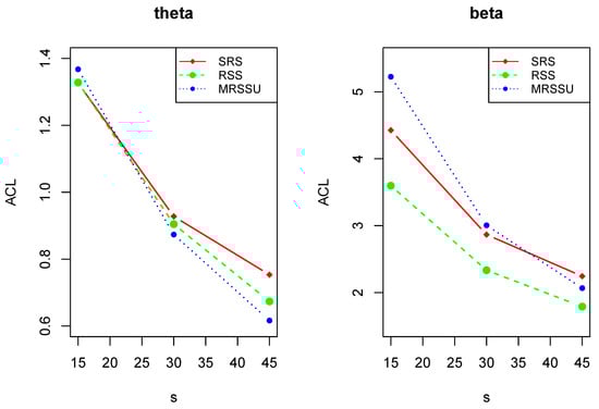
Figure 2. The plots of the ACLs of maximum likelihood interval estimations of $\theta$ and $\beta$.

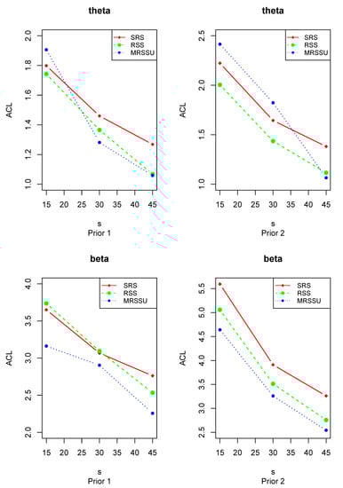
Figure 3. The plots of the ACLs of Bayes interval estimations of $\theta$ and $\beta$.

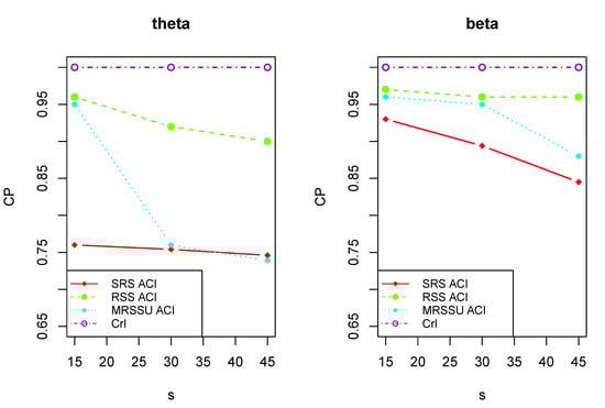
Figure 4. The plots of the CPs of $\theta$ and $\beta$.

6. Data Analysis

Here, an open access dataset from the California Data Exchange Center is illustrated, which can be found in [31]. It is related to the monthly water capacity from the Shasta Reservoir in California, USA, between August and December from 1975 to 2016. The set of data, previously used by some authors such as [11,32], contains a total of 42 observations, which is given in Table 9.

Table 9. The real dataset.

0.667157	0.287785	0.126977	0.768563	0.703119	0.729986	0.767135
0.811159	0.829569	0.726164	0.423813	0.715158	0.640395	0.363365
0.463726	0.371904	0.291172	0.414087	0.650691	0.538082	0.744887
0.722613	0.561238	0.813964	0.709025	0.668612	0.524947	0.606039
0.715850	0.529518	0.824860	0.742025	0.468782	0.345075	0.425334
0.767070	0.679829	0.613911	0.461618	0.294834	0.392917	0.688100

For evaluating the proposed point estimators and interval estimators based on SRS, RSS and MRSSU, we designed $s=12,m=3$ and $n=4$. Use different sampling methods and draw a random sample of size 12. In the case of SRS, a random sample of size 12 is directly drawn. In the case of RSS and MRSSU, three sample sets of size 3 are drawn primarily and some components are selected with iterations according to the specific procedure described in Section 3 and Section 4.

We consider the $90\%$ CIs and a non-information prior, i.e., $({\mu }_1,v_1)=(0,0),$ $({\mu }_2,v_2)=(0,0)$. Then, maximum likelihood point and interval estimation, Bayesian point and interval estimation are given with the results are summarized in Table 10 and Table 11.

Table 10. The point estimates of $\theta$ and $\beta$.

	Point Estimates		Point Estimates
${\widehat{\theta }}_{MLE.SRS}$	2.832703	${\widehat{\beta }}_{MLE.SRS}$	2.190995
${\widehat{\theta }}_{MLE.RSS}$	2.145644	${\widehat{\beta }}_{MLE.RSS}$	1.724308
${\widehat{\theta }}_{MLE.MRSSU}$	2.532715	${\widehat{\beta }}_{MLE.MRSSU}$	2.775230
${\widehat{\theta }}_{BE.SE.SRS}^{\ast }$	2.806827	${\widehat{\beta }}_{BE.SE.SRS}^{\ast }$	2.339172
${\widehat{\theta }}_{BE.SE.RSS}^{\ast }$	2.145149	${\widehat{\beta }}_{BE.SE.RSS}^{\ast }$	1.797477
${\widehat{\theta }}_{BE.SE.MRSSU}^{\ast }$	2.380317	${\widehat{\beta }}_{BE.SE.MRSSU}^{\ast }$	2.692457
${\widehat{\theta }}_{BE.GE.SRS}^{\ast }(k=0.2)$	2.565881	${\widehat{\beta }}_{BE.GE.SRS}^{\ast }(k=0.2)$	1.996350
${\widehat{\theta }}_{BE.GE.RSS}^{\ast }(k=0.2)$	2.014902	${\widehat{\beta }}_{BE.GE.RSS}^{\ast }(k=0.2)$	1.630882
${\widehat{\theta }}_{BE.GE.MRSSU}^{\ast }(k=0.2)$	2.212830	${\widehat{\beta }}_{BE.GE.MRSSU}^{\ast }(k=0.2)$	2.443375
${\widehat{\theta }}_{BE.GE.SRS}^{\ast }(k=0.8)$	2.438731	${\widehat{\beta }}_{BE.GE.SRS}^{\ast }(k=0.8)$	1.843767
${\widehat{\theta }}_{BE.GE.RSS}^{\ast }(k=0.8)$	1.945485	${\widehat{\beta }}_{BE.GE.RSS}^{\ast }(k=0.8)$	1.551529
${\widehat{\theta }}_{BE.GE.MRSSU}^{\ast }(k=0.8)$	2.120080	${\widehat{\beta }}_{BE.GE.MRSSU}^{\ast }(k=0.8)$	2.325173

Table 11. The interval estimates of $\theta$ and $\beta$.

		$90\%$ ACI	Length	$90\%$ CrI	Length
$\theta$	SRS	(1.949037, 3.712106)	1.763069	(1.257362, 4.639019)	3.381657
	RSS	(1.377963, 2.909622)	1.531659	(1.114736, 3.288691)	2.173955
	MRSSU	(1.309699, 2.977556)	1.667856	(1.180012, 3.700654)	2.520642
$\beta$	SRS	(0.898255, 3.483736)	2.585480	(0.847866, 4.571152)	3.723286
	RSS	(0.727022, 2.721594)	1.994572	(0.851320, 3.198368)	2.347048
	MRSSU	(0.640762, 2.807854)	2.167092	(1.268287, 4.776766)	3.508479

7. Conclusions

In this paper, based on Kumaraswamy distribution, point estimations and corresponding interval estimations of unknown parameters grounded on SRS, RSS and MRSSU were investigated by the use of the maximum likelihood approach and Bayes approach. From the perspective of Bayes estimation, we consider squared error and general entropy loss functions. Furthermore, a simulation experiment was illustrated for the purpose of comparing the proposed point estimator (in terms of biases, estimated risks, relative efficiency) and the interval estimator (in the sense of average lengths and coverage percentages).

From numerical outcomes, our first suggestion is to adopt the ranked set sampling scheme, and the second is the simple random sampling scheme, generally. In addition, the Bayes estimators under the squared error loss function outperform the maximum likelihood estimators and Bayes estimators which are under the general entropy loss function. We also focus on a set of real-life data.

In the future, some other problems concerning the Kumaraswamy distribution and the ranked set sample can be further studied, such as the estimations for Kumaraswamy distribution based on the ranked set sample under type I and type II censoring or progressive hybrid censoring.

References

- Kumaraswamy, P. A generalized probability density function for double-bounded random processes. J. Hydrol. 2008, 46, 79–88. [Google Scholar] [CrossRef]
- Jones, M.C. Kumaraswamy’s distribution: A beta-type distribution with some tractability advantages. Stat. Methodol. 2009, 6, 70–81. [Google Scholar] [CrossRef]
- Ponnambalam, K.; Seifi, A.; Vlach, J. Probabilistic design of systems with general distributions of parameters. J. Abbr. 2001, 29, 527–536. [Google Scholar] [CrossRef]
- Dey, S.; Mazucheli, J.; Nadarajah, S. Kumaraswamy distribution: Different methods of estimation. Comput. Appl. Math. 2018, 37, 2094–2111. [Google Scholar] [CrossRef]
- Sindhu, T.N.; Feroze, N.; Aslam, M. Bayesian analysis of the Kumaraswamy distribution under failure censoring sampling scheme. Int. J. Adv. Sci. Technol. 2013, 51, 39–58. [Google Scholar]
- Abd El-Monsef, M.M.E.; Hassanein, W.A.A.E.L. Assessing the lifetime performance index for Kumaraswamy distribution under first-failure progressive censoring scheme for ball bearing revolutions. Qual. Reliab. Eng. Int. 2020, 36, 1086–1097. [Google Scholar] [CrossRef]
- Gholizadeh, R.; Khalilpor, M.; Hadian, M. Bayesian estimations in the Kumaraswamy distribution under progressively type II censoring data. Int. J. Eng. Sci. Technol. 2011, 3, 47–65. [Google Scholar] [CrossRef] [Green Version]
- Sultana, F.; Tripathi, Y.M.; Rastogi, M.K.; Wu, S.J. Parameter estimation for the Kumaraswamy distribution based on hybrid censoring. Am. J. Math. Manag. Sci. 2018, 37, 243–261. [Google Scholar] [CrossRef]
- Kohansal, A.; Nadarajah, S. Stress–strength parameter estimation based on type-II hybrid progressive censored samples for a Kumaraswamy distribution. IEEE Trans. Reliab. 2019, 68, 1296–1310. [Google Scholar] [CrossRef]
- Sultana, F.; Tripathi, Y.M.; Wu, S.J.; Sen, T. Inference for Kumaraswamy Distribution Based on Type I Progressive Hybrid Censoring. Ann. Data Sci. 2020, 1–25. [Google Scholar] [CrossRef]
- Tu, J.; Gui, W. Bayesian Inference for the Kumaraswamy Distribution under Generalized Progressive Hybrid Censoring. Entropy 2020, 22, 1032. [Google Scholar] [CrossRef]
- Saulo, H.; Leão, J.; Bourguignon, M. The kumaraswamy birnbaum-saunders distribution. J. Stat. Theory Pract. 2012, 6, 745–759. [Google Scholar] [CrossRef]
- Iqbal, Z.; Tahir, M.M.; Riaz, N.; Ali, S.A.; Ahmad, M. Generalized Inverted Kumaraswamy Distribution: Properties and Application. Open J. Stat. 2017, 7, 645. [Google Scholar] [CrossRef] [Green Version]
- Khan, M.S.; King, R.; Hudson, I.L. Transmuted kumaraswamy distribution. Stat. Transit. New Ser. 2016, 17, 183–210. [Google Scholar] [CrossRef]
- McIntyre, G.A. A method for unbiased selective sampling, using ranked sets. Aust. J. Agric. Res. 1952, 3, 385–390. [Google Scholar] [CrossRef]
- McIntyre, G.A. Ranked set sampling: Ranking error models and estimation of visual judgment error variance. Biom. J. J. Math. Methods Biosci. 2004, 46, 255–263. [Google Scholar]
- Al-Saleh, M.F.; Al-Hadrami, S.A. Parametric estimation for the location parameter for symmetric distributions using moving extremes ranked set sampling with application to trees data. Environmetrics Off. J. Int. Environmetrics Soc. 2003, 14, 651–664. [Google Scholar] [CrossRef]
- Mahmood, T. On developing linear profile methodologies: A ranked set approach with engineering application. J. Eng. Res. 2020, 8, 203–225. [Google Scholar]
- Sevil, Y.C.; Yildiz, T.Ö. Performances of the Distribution Function Estimators Based on Ranked Set Sampling Using Body Fat Data. Türkiye Klin. Biyoistatistik 2020, 12, 218–228. [Google Scholar] [CrossRef]
- Bocci, C.; Petrucci, A.; Rocco, E. Ranked set sampling allocation models for multiple skewed variables: An application to agricultural data. Environ. Ecol. Stat. 2010, 17, 333–345. [Google Scholar] [CrossRef]
- Biradar, B.S.; Santosha, C.D. Estimation of the mean of the exponential distribution using maximum ranked set sampling with unequal samples. Open J. Stat. 2014, 4, 641. [Google Scholar] [CrossRef] [Green Version]
- Provost, F.; Fawcett, T. Data science and its relationship to Big Data and data-driven decision making. Big Data 2013, 1, 51–59. [Google Scholar] [CrossRef]
- Liang, F.; Paulo, R.; Molina, G.; Clyde, M.A.; Berger, J.O. Mixtures of g priors for Bayesian variable selection. J. Am. Stat. Assoc. 2008, 103, 410–423. [Google Scholar] [CrossRef]
- Caraka, R.E.; Yusra, Y.; Toharudin, T.; Chen, R.C.; Basyuni, M.; Juned, V.; Gio, P.U.; Pardamean, B. Did Noise Pollution Really Improve during COVID-19? Evidence from Taiwan. Sustainability 2021, 13, 5946. [Google Scholar] [CrossRef]
- Salimans, T.; Kingma, D.; Welling, M. Markov chain monte carlo and variational inference: Bridging the gap. In Proceedings of the 32nd International Conference on Machine Learning, Lille, France, 7–9 July 2015; pp. 1218–1226. [Google Scholar]
- Dellaportas, P.; Forster, J.J.; Ntzoufras, I. On Bayesian model and variable selection using MCMC. Stat. Comput. 2002, 12, 27–36. [Google Scholar] [CrossRef]
- Caraka, R.E.; Nugroho, N.T.; Tai, S.K.; Chen, R.C.; Toharudin, T.; Pardamean, B. Feature importance of the aortic anatomy on endovascular aneurysm repair (EVAR) using Boruta and Bayesian MCMC. Commun. Math. Biol. Neurosci. 2020. [Google Scholar] [CrossRef]
- Rabinovich, M.; Angelino, E.; Jordan, M.I. Variational consensus monte carlo. arXiv 2015, arXiv:1506.03074. [Google Scholar]
- Biradar, B.S.; Santosha, C.D. Point estimation under asymmetric loss functions for left-truncated exponential samples. Commun. Stat. Theory Methods 1996, 25, 585–600. [Google Scholar]
- Brooks, S.; Gelman, A.; Jones, G.; Meng, X.L. (Eds.) Handbook of Markov Chain Monte Carlo; Chapman & Hall/CRC: Boca Raton, FL, USA, 2011. [Google Scholar]
- Query Monthly CDEC Senser Values. Available online: http://cdec.water.ca.gov/dynamicapp/QueryMonthly?SHA (accessed on 19 June 2021).
- Kohansal, A. On estimation of reliability in a multicomponent stress-strength model for a Kumaraswamy distribution based on progressively censored sample. Stat. Pap. 2019, 60, 2185–2224. [Google Scholar] [CrossRef]
Publisher’s Note: MDPI stays neutral with regard to jurisdictional claims in published maps and institutional affiliations. |
© 2021 by the authors. Licensee MDPI, Basel, Switzerland. This article is an open access article distributed under the terms and conditions of the Creative Commons Attribution (CC BY) license (https://creativecommons.org/licenses/by/4.0/).