An Efficient Mechanism to Solve Fractional Differential Equations Using Fractional Decomposition Method

Abstract

We present some new results that deal with the fractional decomposition method (FDM). This method is suitable to handle fractional calculus applications. We also explore exact and approximate solutions to fractional differential equations. The Caputo derivative is used because it allows traditional initial and boundary conditions to be included in the formulation of the problem. This is of great significance for large-scale problems. The study outlines the significant features of the FDM. The relation between the natural transform and Laplace transform is a symmetrical one. Our work can be considered as an alternative to existing techniques, and will have wide applications in science and engineering fields.

1. Introduction

For many years the subject of fractional calculus has been studied by many research scholars. This is an ongoing process and one can recognizes that within the field for this study of fractional calculus new techniques and mechanisms show up, which in turn make it possible, to find important challenging insights and unknown correlations between many areas of physics. Recently, an increase in the interest of scientist in non-local field theories. In order for us to deal with problems in high-energy and particle physics which only up to this point can be done with local field theories, there is a valid reason for these late developments. Fractional derivatives have proven their capability to describe several phenomena associated with memory and after effects due to their non-locality property [1,2]. Such phenomena are commonplace in physical processes, biological structures, and cosmological problems. For example, the fractional rheological models have been employed to test the low applied force frequencies [3,4,5,6]. For this reason, it became necessary to illuminate the solutions of the models that describe these phenomena. Several analytical techniques are presented to achieve their objectives. Actually, all these approaches are accommodation for the existing methods to handle the integer case models, which is natural since the fractional derivative generalizes the classical derivative to an arbitrary order.

Recently, fractional calculus and their applications have been treated by many researchers, see [5,6,7,8,9,10,11,12,13] and the references therein. Even though fractional derivatives have existed as long as their integer order counterparts, only in recent decades have fractional derivative models become exciting new tools in the study of practical problems in disciplines as diverse as physics [14,15,16], finance [14,17], biology [6,7] and hydrology [4,10,18,19]. As fractional derivative models are becoming increasingly popular among the wider scientific community, it becomes the main motivation to study numerical schemes for fractional differential equations. Lately, many techniques have discussed the means of exploring approximate solutions of fractional differential equations, such as finite difference and finite element method (FDFEM) [20], spectral method [21] the fractional sub-equation method [10], the fast and parallel computational methods (FPCM) [15,16], the fractional variation method (FVM) [5], the fractional complex transform (FCT) [22], fractional Laplace method [23] and the fractional Adomian decomposition method (FADM) [19,24]. We will use fractional natural decomposition method (FNDM) to solve FODEs and fractional system of ODEs. The method was proven to converge rapidly, and the existence and uniqueness of the method was proven in [25].

Because of the nonstop needs for another new schemes that exist in the literature, e.g. the Mellin transform, and its relation to transforms namely the Sumudu transform and the Al Zaki transform, we developed a valid mechanism which we called the fractional decomposition method (FDM) to find solutions to fractional nonlinear ODEs and PDEs including systems of FDEs. Our scheme avoids the computational difficulties we usually face in other methods exist in the literature, which usually use linearization, discretization and perturbation schemes. Moreover, we have given detailed proofs to some theorems using the proposed method FDM. Also, we presented some important examples of systems fractional differential equations and showed that the FDM provide solutions, which coincide with the ones done by other researchers. To name one, is the solution of diffusion equation with fractional derivatives. These are appeared in Section 4.

Our work will be presented in the following manner: First, in Section 2, we give the history of the natural transform method, and definitions of fractional derivatives. In Section 3, we present proofs to results related to the natural fractional derivatives. Section 4 is devoted to the applications model of FDEs using the proposed method. In Section 5, we solve fractional systems of ODEs. Finally, our concluding remarks are presented, in Acknowledgment, where we outline what we have accomplished in this research.

2. Related Materials

We explore some definitions and terminologies of the natural transform that will be needed later on in the proofs of our results, (see, for example, [14,17,26]).

Definition 1.

Suppose $h\left(x\right)$ is a real function, where $x>0$. Then $h\left(x\right)$ is said to be in the space $C_{\mu }$, where μ is areal number, if $\exists q\in \mathbb{R}$ with $q>\mu$, such that $h\left(x\right)=x^{q}g\left(x\right)$, where $g\left(x\right)\in C\left[0,\infty \right)$, and it is said to be in the space $C_{\mu }^m$ if $h^{\left(m\right)}\in C_{\mu },m\in \mathbb{N}$.

Definition 2.

Let $k-1<\upsilon \le k,k\in \mathbb{N},y>0,\phi \in C_{-1}^k$. The fractional derivative of f in the Caputo sense can be defined as

$${}^c{D}^{\upsilon }\phi \left(y\right)=J^{k-\upsilon }{D}^k\phi \left(y\right)=\frac{1}{\mathsf{\Gamma }(\upsilon -k)}{\int }_0^y{(y-t)}^{k-\upsilon -1}{\phi }^{\left(k\right)}\left(t\right)dt.$$

(1)

Definition 3.

Refs. [27,28] The two–parameter Mittag–Leffler function is given by

${\displaystyle E_{\upsilon ,\eta }\left(z\right)=\sum _{k=0}^{\infty }\frac{z^k}{\mathsf{\Gamma }(\upsilon k+\eta )},\upsilon >0,\eta >0,z\in \mathbb{C}.}$

Next, we define the natural transform (N-transform) along with the definition of exponential order function following [23].

Definition 4.

Let $h\left(t\right)$ be a function piecewise continuous, with bounded variation, locally integrable (i.e., the function is absolutely integrable in any real interval $[a,b]$ so that ${\int }_a^b\left|h\left(t\right)\right|dt<\infty$), and of exponential order, then there exists the N-transform of $h\left(t\right)$. That is, a function of exponential order is the one that does not “grow faster” than given exponentials, as $t⟶\pm \infty$. Alternatively, there are real constants $K,a>0$ such that $\left|h\left(t\right)\right|<K·e^{at}$, when t is large and negative (say, for $t<t_1\in \mathbb{R}$). In addition, there are real constants $M,b>0$ such that $\left|h\left(t\right)\right|<M·e^{bt}$, when t is large (say, for $t>t_1\in \mathbb{R}$). It also has to be true that $b<a$.

Then, we define the natural transform

$$\mathcal{N}\left(h\left(t\right)\right)=R(s,u)={\int }_{-\infty }^{\infty }{e}^{-st}h\left(ut\right)dy,s,u\in (-\infty ,\infty ),$$

(2)

where $\mathcal{N}$ is the N-transform of $h\left(t\right)$ and s and u are the N-transform variables. Note that one can writes Equation (2) as

$$\mathcal{N}\left(h\left(t\right)\right)=R^{-}(s,u)+R^{+}(s,u).$$

Hence,

$${\mathcal{N}}^{+}\left(h\left(t\right)\right)=R^{+}(s,u)=\frac{1}{u}{\int }_0^{\infty }{e}^{-\frac{st}{u}}h\left(t\right)dt,s,u\in (0,\infty ).$$

(3)

Remark 1.

Under these conditions, when $R(s,u)$ is analytic, the integral in Equation (2) converges uniformly and absolutely in the complex plane defined by the strip $b<Re\left(s\right)<a$.

Note that one can obtain the Laplace transform and the Sumudu transform if we plug in $u=1$, and $s=1$ in the above equations, respectively. Hence, the relation between the natural transform and Laplace transform is a symmetry one.

We shall use the well-known gamma function throughout this paper

$$\mathsf{\Gamma }\left(z\right)={\int }_0^{\infty }{e}^{-t}{t}^{z-1}dt,z>0,$$

(4)

where $\mathsf{\Gamma }\left(z+1\right)=z\mathsf{\Gamma }\left(z\right)$.

Important Properties

Here are some of the main properties for the N-transforms which can be found in [26].

Property 1.

${\mathcal{N}}^{+}\left(1\right)=\frac{1}{s},Re\left(s\right)>0$.

Property 2.

${\mathcal{N}}^{+}\left(y^{\upsilon }\right)=\frac{\mathsf{\Gamma }(\upsilon +1)u^{\upsilon }}{s^{\upsilon +1}},\upsilon >-1,Re\left(s\right)>0.$

Property 3.

${\mathcal{N}}^{+}\left({}^c{D}_t^{\upsilon }\phi \left(t\right)\right)(s,u)=\frac{s^{\upsilon }}{u^{\upsilon }}{\mathcal{N}}^{+}\left(\phi \left(t\right)\right)(s,u)-\frac{s^{\upsilon -1}}{u^{\upsilon }}\phi \left(0\right),Re\left(s\right)>0.$

3. Natural Caputo Fractional Derivatives

Here, we give detailed proofs to some theorems of N-transform of Caputo fractional derivative. The proof of theorem 1 was given in another published paper by the first author.

Caputo Fractional Derivative

For the sake of readers, we give just some of the natural transform properties. For more properties, we direct the reader to see, for example, [15,16,26].

Theorem 1.

If $k\in {\mathbb{Z}}^{+}$, where $k-1\le \upsilon <k$. Then, the N-transform of Caputo derivative of $\phi \left(t\right)$ is

$${\mathcal{N}}^{+}\left({}^c{D}_t^{\upsilon }\phi \left(t\right)\right)=\frac{s^{\upsilon }}{u^{\upsilon }}R(s,u)-\sum _{m=0}^{k-1}\frac{s^{\upsilon -(m+1)}}{u^{\upsilon -m}}{\left(D^m\phi \left(t\right)\right)}_{t=0}.$$

(5)

Theorem 2.

The natural transform of the Caputo derivative for $\phi \left(t\right)=1$ is given by

$${\mathcal{N}}^{+}\left({}^c{D}_t^{\upsilon }\left(1\right)\right)=0.$$

Proof. 

From Equation (5), we have

$$\begin{array}{cc}\hfill {\mathcal{N}}^{+}\left({}^c{D}_t^{\upsilon }\left(1\right)\right)& =\frac{s^{\upsilon }}{u^{\upsilon }}{\mathcal{N}}^{+}\left(1\right)-\sum _{m=0}^{k-1}\frac{s^{\upsilon -(m+1)}}{u^{\upsilon -m}}{\left(D^m\phi \left(t\right)\right)}_{t=0}\hfill \\ \hfill & =\frac{s^{\upsilon }}{u^{\upsilon }}\frac{1}{s}-\frac{s^{\upsilon -1}}{u^{\upsilon }}\left[1\right]-0\hfill \\ \hfill & =\frac{s^{\upsilon -1}}{u^{\upsilon }}-\frac{s^{\upsilon -1}}{u^{\upsilon }}\hfill \\ \hfill & =0.\hfill \end{array}$$

□

Theorem 3.

(a) The natural transform of the Caputo derivative for $\phi \left(t\right)=t$ with $0<\upsilon \le 1$ is given by

$${\mathcal{N}}^{+}\left({}^c{D}_t^{\upsilon }\left(t\right)\right)=\frac{s^{\upsilon -2}}{u^{\upsilon -1}}.$$

(b) 

The natural transform of the Caputo derivative for $\phi \left(t\right)=t$ with $k-1<\upsilon \le k$, and $k=2,3,4,\dots$ is

$${\mathcal{N}}^{+}\left({}^c{D}_t^{\upsilon }\left(t\right)\right)=0.$$

Proof. 

First note that $f^{\prime }\left(t\right)=1,f^{″}\left(t\right)=0,\dots ,f^{(k-1)}\left(t\right)=0$.

Case 1.  $0<\upsilon \le 1$. From Equation (5), we have

$$\begin{array}{cc}\hfill {\mathcal{N}}^{+}\left({}^c{D}_t^{\upsilon }\left(t\right)\right)& =\frac{s^{\upsilon }}{u^{\upsilon }}{\mathcal{N}}^{+}\left(t\right)-\sum _{m=0}^{k-1}\frac{s^{\upsilon -(m+1)}}{u^{\upsilon -m}}{\left(D^m\phi \left(t\right)\right)}_{t=0}\hfill \\ \hfill & =\frac{s^{\upsilon }}{u^{\upsilon }}\frac{u}{s^2}-\frac{s^{\upsilon -1}}{u^{\upsilon }}\left[0\right]\hfill \\ \hfill & =\frac{s^{\upsilon -2}}{u^{\upsilon -1}}.\hfill \end{array}$$

Case 2.  $k-1<\upsilon \le k$, and $k=2,3,4,\dots .$

We get from Equation (5),

$$\begin{array}{cc}\hfill {\mathcal{N}}^{+}\left({}^c{D}_t^{\upsilon }\left(t\right)\right)& =\frac{s^{\upsilon }}{u^{\upsilon }}{\mathcal{N}}^{+}\left(t\right)-\sum _{m=0}^{k-1}\frac{s^{\upsilon -(m+1)}}{u^{\upsilon -m}}{\left(D^m\phi \left(t\right)\right)}_{t=0}\hfill \\ \hfill & =\frac{s^{\upsilon }}{u^{\upsilon }}\frac{u}{s^2}-\frac{s^{\upsilon -1}}{u^{\upsilon }}\left[0\right]-\frac{s^{\upsilon -2}}{u^{\upsilon -1}}\left[1\right]-\cdots -\frac{s^{\upsilon -n}}{u^{\upsilon -n+1}}\left[0\right]\hfill \\ \hfill & =\frac{s^{\upsilon -2}}{u^{\upsilon -1}}-\frac{s^{\upsilon -2}}{u^{\upsilon -1}}\hfill \\ \hfill & =0.\hfill \end{array}$$

□

Theorem 4.

The natural transform of the Caputo derivative for $\phi \left(t\right)=\frac{t^{k-1}}{k!}$ is

$${\mathcal{N}}^{+}\left({}^c{D}_t^{\upsilon }\left(\frac{t^{k-1}}{k!}\right)\right)=\frac{s^{\upsilon -k}}{k{u}^{\upsilon -k+1}},$$

with $k=3,4,\dots .$

Proof. 

First note that

$$f^{\prime }\left(t\right)=\frac{(k-1)t^{k-2}}{k!},f^{″}\left(t\right)=\frac{(k-1)(k-2)t^{k-3}}{k!},\dots ,f^{(n-1)}\left(t\right)={\frac{(k-1)(k-2)\dots (k-n+1)t}{k!}}^{k-n}.$$

One can conclude from Equation (5),

$$\begin{array}{ccc}\hfill \mathcal{N}{}^{+}\left({}^c{D}_t^{\upsilon }\left(\frac{t^{k-1}}{k!}\right)\right)& =& {\displaystyle \frac{s^{\upsilon }}{u^{\upsilon }}{\mathcal{N}}^{+}\left[\frac{t^{k-1}}{k!}\right]-\sum _{j=0}^{n-1}\frac{s^{\upsilon -(j+1)}}{u^{\upsilon -j}}{\left[D^j\phi \left(t\right)\right]}_{t=0}}\hfill \\ \\ \hfill & =& \frac{s^{\upsilon }}{u^{\upsilon }}\frac{u^{k-1}}{k{s}^k}-\left(0+0+\dots +0\right)\hfill \\ \\ \hfill & =& \frac{s^{\upsilon -k}}{k{u}^{\upsilon -k+1}}.\hfill \end{array}$$

□

Theorem 5.

The natural transform of the Caputo derivative for $\phi \left(t\right)=e^{at}$ is

$${\mathcal{N}}^{+}\left({}^c{D}_t^{\upsilon }\left(e^{at}\right)\right)=\frac{a^n{u}^n{s}^{\upsilon -n}}{u^{\upsilon }\left(s-au\right)}.$$

Proof. 

First note that ${\phi }^{\prime }\left(t\right)=a{e}^{at},{\phi }^{″}\left(t\right)=a^2{e}^{at},\dots ,{\phi }^{(n-1)}\left(t\right)=a^{n-1}{e}^{at}$. Then, we get

$$\begin{array}{ccc}\hfill {\mathcal{N}}^{+}\left({}^c{D}_t^{\upsilon }\left(e^{at}\right)\right)& =& {\displaystyle \frac{s^{\upsilon }}{u^{\upsilon }}{\mathcal{N}}^{+}\left(e^{at}\right)-\sum _{k=0}^{n-1}\frac{s^{\upsilon -(k+1)}}{u^{\upsilon -k}}{D}^k{\left(\phi \left(t\right)\right)}_{t=0}}\hfill \\ \\ \hfill & =& \frac{s^{\upsilon }}{u^{\upsilon }}\frac{1}{s-au}-\left[\frac{s^{\upsilon -1}}{u^{\upsilon }}+\frac{s^{\upsilon -2}}{u^{\upsilon -1}}a+\dots +\frac{s^{\upsilon -n}}{u^{\upsilon -n+1}}{a}^{n-1}\right]\hfill \\ \\ \hfill & =& \frac{s^{\upsilon }}{u^{\upsilon }}\frac{1}{s-au}-\left[\frac{s^{\upsilon -1}}{u^{\upsilon }}+\frac{s^{(\upsilon -1)-1}}{u^{\upsilon -1}}a+\dots +\frac{s^{(\upsilon -1)-(n-1)}}{u^{\upsilon -(n-1)}}{a}^{n-1}\right]\hfill \\ \\ \hfill & =& \frac{s^{\upsilon }}{u^{\upsilon }}\frac{1}{s-au}-\sum _{k=0}^{n-1}\frac{s^{(\upsilon -1)-k}}{u^{\upsilon -k}}{a}^k\hfill \\ \\ \hfill & =& \frac{a^n{u}^n{s}^{\upsilon -n}}{u^{\upsilon }\left(s-au\right)}.\hfill \end{array}$$

□

Theorem 6.

The Caputo Fractional Natural Transform of $f\left(t\right)=\frac{e^{bt}-e^{at}}{b-a},a\ne b$ is

$${\mathcal{N}}^{+}\left[{}^c{D}^{\alpha }\left(\frac{e^{bt}-e^{at}}{b-a}\right)\right]=\frac{s^{\alpha +1-n}{u}^{n-\alpha }(b^n-a^n)+u^{n+1-\alpha }{s}^{\alpha -n}(a^{n}b-b^{n}a)}{(b-a)(s-ub)(s-ua)}$$

Proof. 

First note that

$$f^{\prime }\left(t\right)=\frac{b{e}^{bt}-a{e}^{at}}{b-a},f^{″}\left(t\right)=\frac{b^2{e}^{bt}-a^2{e}^{at}}{b-a},\cdots ,f^{(n-1)}\left(t\right)=\frac{b^{n-1}{e}^{bt}-a^{n-1}{e}^{at}}{b-a}.$$

$$\begin{array}{cc}\hfill {\mathcal{N}}^{+}\left[{}^c{D}^{\alpha }\left(\frac{e^{bt}-e^{at}}{b-a}\right)\right]& =\frac{s^{\alpha }}{u^{\alpha }}{}^{+}\left[\frac{e^{bt}-e^{at}}{b-a}\right]-\sum _{k=0}^{n-1}\frac{s^{\alpha -(k+1)}}{u^{\alpha -k}}{\left[D^{k}f\left(t\right)\right]}_{t=0}\hfill \\ \hfill & =\frac{s^{\alpha }}{u^{\alpha }}\frac{u}{(s-au)(s-bu)}-\left[\frac{s^{\alpha -2}}{u^{\alpha -1}}\frac{b-a}{b-a}+\cdots +\frac{s^{\alpha -n}}{u^{\alpha -n+1}}\frac{b^{n-1}-a^{n-1}}{b-a}\right]\hfill \\ & =\frac{u^{1-\alpha }{s}^{\alpha }}{(s-au)(s-bu)}-\frac{1}{b-a}\left[\frac{\mp s^{\alpha -1}}{u^{\alpha }}+\cdots +\frac{s^{\alpha -n}}{u^{\alpha -(n-1)}}(b^{n-1}-a^{n-1})\right]\hfill \\ & =\frac{u^{1-\alpha }{s}^{\alpha }}{(s-au)(s-bu)}-\frac{1}{b-a}\sum _{k=0}^{n-1}\frac{s^{\alpha -(k+1)}}{u^{\alpha -k}}(b^k-a^k)\hfill \\ & =\frac{s^{\alpha }}{u^{\alpha }}\frac{u}{(s-au)(s-bu)}-\frac{s^{\alpha -1}}{u^{\alpha }(b-a)}\sum _{k=0}^{n-1}{\left(\frac{ub}{s}\right)}^k+\frac{s^{\alpha -1}}{u^{\alpha }(b-a)}\sum _{k=0}^{n-1}{\left(\frac{ua}{s}\right)}^k\hfill \\ & =\frac{s^{\alpha }}{u^{\alpha }}\frac{u}{(s-au)(s-bu)}-\frac{s^{\alpha -1}}{u^{\alpha }(b-a)}\frac{1-{\left(\frac{ub}{s}\right)}^n}{1-\frac{ub}{s}}+\frac{s^{\alpha -1}}{u^{\alpha }(b-a)}\frac{1-{\left(\frac{ua}{s}\right)}^n}{1-\frac{ua}{s}}\hfill \\ & =\frac{s^{\alpha +1-n}{u}^{n-\alpha }(b^n-a^n)+u^{n+1-\alpha }{s}^{\alpha -n}(a^{n}b-b^{n}a)}{(b-a)(s-ub)(s-ua)}.\hfill \end{array}$$

(6)

□

Applications of FDM for Fractional ODEs and PDEs

Here we employ the new scheme to solve two non-linear fractional ODEs and we present solution to the diffusion fractional differential equations. Finally, we develop numerical tables for these examples for multiple values of $\upsilon$ and t.

Methodology of FDM

Consider the general nonlinear (FODE)

$${}^c{D}_t^{\upsilon }y\left(t\right)+L\left(y\left(t\right)\right)+F\left(y\left(t\right)\right)=g\left(t\right),$$

(7)

where $t>0$ and $0<\upsilon \le 1$, and along with initial condition

$$y\left(0\right)=y_0,$$

(8)

where ${}^c{D}_t^{\upsilon }y\left(t\right)$ is the Caputo derivative for $y\left(t\right)$, L is the linear differential operator and F represents the nonlinear part. Also $g\left(t\right)$ is the non-homogeneous part, and $y_0$ is defined and continuous.

We can conclude by applying Theorem 1 to Equation (6)

$${\mathcal{N}}^{+}\left(y\left(t\right)\right)=\frac{u^{\upsilon }}{s^{\upsilon }}\sum _{k=0}^{n-1}\frac{s^{\upsilon -(k+1)}}{u^{\upsilon -k}}{D}^k{\left(y\left(t\right)\right)}_{t=0}+\frac{u^{\upsilon }}{s^{\upsilon }}{\mathcal{N}}^{+}\left(g\left(t\right)\right)-\frac{u^{\upsilon }}{s^{\upsilon }}{\mathcal{N}}^{+}\left(L\left(y\left(t\right)\right)+\left(Fy\left(t\right)\right)\right).$$

(9)

Substituting Equation (7) into Equation (8) and then taking ${\mathcal{N}}^{-1}$, one can conclude

$$\begin{array}{ccc}\hfill y\left(t\right)& =& {\mathcal{N}}^{-1}\left(\frac{y_0}{s}\right)+{\mathcal{N}}^{-1}\left(\frac{u^{\upsilon }}{s^{\upsilon }}{\mathcal{N}}^{+}\left(g\left(t\right)\right)\right)-{\mathcal{N}}^{-1}\left(\frac{u^{\upsilon }}{s^{\upsilon }}{\mathcal{N}}^{+}\left(L\left(y\left(t\right)\right)+F\left(y\left(t\right)\right)\right)\right)\hfill \\ \\ \hfill & =& H\left(t\right)-{\mathcal{N}}^{-1}\left(\frac{u^{\upsilon }}{s^{\upsilon }}{\mathcal{N}}^{+}\left(L\left(y\left(t\right)\right)+F\left(y\left(t\right)\right)\right)\right),\hfill \end{array}$$

(10)

where $H\left(t\right)$ is arising from the non-homogeneous part together with the initial condition. Assuming a solution exist of $y\left(t\right)$ as follows

$$y\left(t\right)=\sum _{n=0}^{\infty }{y}_n\left(t\right).$$

(11)

But the nonlinear part in our problem is

$$F\left(y\left(t\right)\right)=\sum _{n=0}^{\infty }{A}_n\left(t\right),$$

(12)

where the Adomian polynomials of $y_0,y_1,\dots y_n$ are computed using

$$A_n=\frac{1}{n!}\frac{d^n}{d{\lambda }^n}{\left[\mathbb{F}\left(\sum _{j=0}^n{\lambda }^i{y}_i\right)\right]}_{\lambda =0},n=0,1,2,\dots$$

(13)

Thus, Equation (12) can be reduced to

$$\begin{array}{c}{A}_0=\mathbb{F}\left(y_0\right)\hfill \\ \\ A_1=y_1{\mathbb{F}}^{\prime }\left(y_0\right)\hfill \\ \\ A_2=y_2{\mathbb{F}}^{\prime }\left(y_0\right)+\frac{1}{2!}{y}_1^2{\mathbb{F}}^{″}\left(y_0\right).\hfill \end{array}$$

(14)

The rest of Adomian polynomials can be obtained likewise. Substituting Equation (11) into Equation (9), one arrives at

$$\sum _{n=0}^{\infty }{y}_n\left(t\right)=H\left(t\right)-{\mathcal{N}}^{-1}\left(\frac{u^{\upsilon }}{s^{\upsilon }}{\mathcal{N}}^{+}\left(L\left(\sum _{n=0}^{\infty }{y}_n\left(t\right)\right)+\sum _{n=0}^{\infty }{A}_n\left(t\right)\right)\right).$$

(15)

One can arrive, with the help of Equation (14), at

$$\begin{array}{c}{y}_0\left(t\right)=G\left(t\right)\hfill \\ \\ y_1\left(t\right)=-{\mathcal{N}}^{-1}\left(\frac{u^{\upsilon }}{s^{\upsilon }}{\mathcal{N}}^{+}\left(L\left(y_0\left(t\right)\right)+A_0\left(t\right)\right)\right)\hfill \\ \\ y_2\left(t\right)=-{\mathcal{N}}^{-1}\left(\frac{u^{\upsilon }}{s^{\upsilon }}{\mathcal{N}}^{+}\left(L\left(y_1\left(t\right)\right)+A_1\left(t\right)\right)\right)\hfill \\ \\ y_3\left(t\right)=-{\mathcal{N}}^{-1}\left(\frac{u^{\upsilon }}{s^{\upsilon }}{\mathcal{N}}^{+}\left(L\left(y_2\left(t\right)\right)+A_2\left(t\right)\right)\right)\hfill \end{array}$$

Eventually, we have the general recursion formula as

$$y_{n+1}\left(t\right)=-{\mathcal{N}}^{-1}\left(\frac{u^{\upsilon }}{s^{\upsilon }}{\mathcal{N}}^{+}\left(L\left(y_n\left(t\right)\right)+A_n\left(t\right)\right)\right),n\ge 1.$$

(16)

Hence, our approximate solution is of the form

$$y\left(t\right)=\sum _{n=0}^{\infty }{y}_n\left(t\right).$$

(17)

Test Problems

Example 1.

Consider the nonlinear FDE in the form

$${}^c{D}_{{}^t}^{\upsilon }\phi \left(t\right)+{\phi }^2\left(t\right)=2\phi \left(t\right)+1,0<\upsilon \le 1,$$

(18)

together with condition

$$y\left(0\right)=0.$$

(19)

Applying Theorem 1 to Equation (17), one arrives at

$$\begin{array}{ccc}\hfill {\mathcal{N}}^{+}\left(\phi \left(t\right)\right)& =& \frac{u^{\upsilon }}{s^{\upsilon }}{\mathcal{N}}^{+}\left(1\right)+2\frac{u^{\upsilon }}{s^{\upsilon }}{\mathcal{N}}^{+}\left(\phi \left(t\right)\right)-\frac{u^{\upsilon }}{s^{\upsilon }}{\mathcal{N}}^{+}\left({\phi }^2\left(t\right)\right)\hfill \\ \\ \hfill & =& \frac{u^{\upsilon }}{s^{\upsilon +1}}+2\frac{u^{\upsilon }}{s^{\upsilon }}{\mathcal{N}}^{+}\left(\phi \left(t\right)\right)-\frac{u^{\upsilon }}{s^{\upsilon }}{\mathcal{N}}^{+}\left({\phi }^2\left(t\right)\right)\hfill \end{array}$$

(20)

Taking the N-transform inverse of Equation (19) one concludes

$$\phi \left(t\right)={\mathcal{N}}^{-1}\left(\frac{u^{\upsilon }}{s^{\upsilon +1}}\right)+2{\mathcal{N}}^{-1}\left(\frac{u^{\upsilon }}{s^{\upsilon }}{\mathcal{N}}^{+}\left(\phi \left(t\right)\right)\right)-{\mathcal{N}}^{-1}\left(\frac{u^{\upsilon }}{s^{\upsilon }}{\mathcal{N}}^{+}\left({\phi }^2\left(t\right)\right)\right).$$

(21)

Suppose a solution exist for $\phi \left(t\right)$ and the nonlinear term ${\phi }^2\left(t\right)$ is given as

$$\phi \left(t\right)=\sum _{n=0}^{\infty }{\phi }_n\left(t\right),{\phi }^2\left(t\right)=\sum _{n=0}^{\infty }{A}_n\left(t\right).$$

(22)

Note here,

$$\begin{array}{c}{A}_0={\left({\phi }_0\right)}^2\hfill \\ \\ A_1=2{\phi }_0{\phi }_1\hfill \\ \\ A_2=2{\phi }_0{\phi }_2+{\left({\phi }_1\right)}^2\hfill \\ \\ A_3=2{\phi }_0{\phi }_3+2{\phi }_1{\phi }_2.\hfill \end{array}$$

Using Equation (21), one notices Equation (20) becomes

$$\phi \left(t\right)=\sum _{n=0}^{\infty }{\phi }_n\left(t\right)={\mathcal{N}}^{-1}\left(\frac{u^{\upsilon }}{s^{\upsilon +1}}\right)+2{\mathcal{N}}^{-1}\left(\frac{u^{\upsilon }}{s^{\upsilon }}{\mathcal{N}}^{+}\left(\phi \left(t\right)\right)\right)-{\mathcal{N}}^{-1}\left(\frac{u^{\upsilon }}{s^{\upsilon }}{\mathcal{N}}^{+}\left({\phi }^2\left(t\right)\right)\right).$$

(23)

Looking at both sides of Equation (22), one can conclude

$${\phi }_0\left(t\right)=\frac{t^{\upsilon }}{\mathsf{\Gamma }\left(\upsilon +1\right)}.$$

$$\begin{array}{ccc}\hfill {\phi }_1\left(t\right)& =& 2{\mathcal{N}}^{-1}\left(\frac{u^{\upsilon }}{s^{\upsilon }}{\mathcal{N}}^{+}\left({\phi }_0\left(t\right)\right)\right)-{\mathcal{N}}^{-1}\left(\frac{u^{\upsilon }}{s^{\upsilon }}{\mathrm{N}}^{+}\left(A_0\right)\right)\hfill \\ \\ \hfill & =& 2{\mathcal{N}}^{-1}\left[\frac{u^{\upsilon }}{s^{\upsilon }}{\mathcal{N}}^{+}\left(\frac{t^{\upsilon }}{\mathsf{\Gamma }\left(\upsilon +1\right)}\right)\right]-\frac{\mathsf{\Gamma }\left(2\upsilon +1\right)}{{\left(\mathsf{\Gamma }\left(\upsilon +1\right)\right)}^2}{\mathcal{N}}^{-1}\left(\frac{u^{\upsilon }}{s^{\upsilon }}{\mathcal{N}}^{+}\left(t^{2\upsilon }\right)\right)\hfill \\ \\ \hfill & =& 2{\mathcal{N}}^{-1}\left(\frac{u^{2\upsilon }}{s^{2\upsilon +1}}\right)-\frac{\mathsf{\Gamma }\left(2\upsilon +1\right)}{{\left(\mathsf{\Gamma }\left(\upsilon +1\right)\right)}^2}{\mathcal{N}}^{-1}\left(\frac{u^{3\upsilon }}{s^{3\upsilon +1}}\right)\hfill \\ \\ \hfill & =& \frac{2}{\mathsf{\Gamma }\left(2\upsilon +1\right)}{t}^{2\upsilon }-\frac{\mathsf{\Gamma }\left(2\upsilon +1\right)}{\mathsf{\Gamma }\left(3\upsilon +1\right){\left(\mathsf{\Gamma }\left(\upsilon +1\right)\right)}^2}{t}^{3\upsilon }.\hfill \end{array}$$

Likewise,

$$\begin{array}{ccc}\hfill \phi {}_2\left(t\right)& =& \frac{4t^{3\alpha }}{\mathsf{\Gamma }\left(3\alpha +1\right)}-\left[\frac{2\mathsf{\Gamma }\left(2\alpha +1\right)}{{\left(\mathsf{\Gamma }\left(\alpha +1\right)\right)}^2}+\frac{4\mathsf{\Gamma }\left(3\alpha +1\right)}{\mathsf{\Gamma }\left(\alpha +1\right)\mathsf{\Gamma }\left(2\alpha +1\right)}\right]\frac{t^{4\alpha }}{\mathsf{\Gamma }\left(4\alpha +1\right)}-\frac{2\mathsf{\Gamma }\left(2\alpha +1\right)\mathsf{\Gamma }\left(4\alpha +1\right)t^{5\alpha }}{{\left(\mathsf{\Gamma }\left(\alpha +1\right)\right)}^3\mathsf{\Gamma }\left(3\alpha +1\right)\mathsf{\Gamma }\left(5\alpha +1\right)}.\hfill \\ \hfill & & \hfill \end{array}$$

$$\begin{array}{ccc}\hfill {\phi }_3\left(t\right)& =& \frac{8t^{4\upsilon }}{\mathsf{\Gamma }\left(4\upsilon +1\right)}-\left(\frac{4\mathsf{\Gamma }\left(2\upsilon +1\right)}{{\left(\mathsf{\Gamma }\left(\upsilon +1\right)\right)}^2}+\frac{8\mathsf{\Gamma }\left(3\upsilon +1\right)}{\mathsf{\Gamma }\left(\upsilon +1\right)\mathsf{\Gamma }\left(2\upsilon +1\right)}\right)\frac{t^{5\upsilon }}{\mathsf{\Gamma }\left(5\upsilon +1\right)}\hfill \\ \\ & -& \frac{4\mathsf{\Gamma }\left(2\upsilon +1\right)\mathsf{\Gamma }\left(4\upsilon +1\right)}{{\left(\mathsf{\Gamma }\left(\upsilon +1\right)\right)}^3\mathsf{\Gamma }\left(3\upsilon +1\right)}\frac{t^{6\upsilon }}{\mathsf{\Gamma }\left(6\upsilon +1\right)}-\left(\frac{8}{\mathsf{\Gamma }\left(\upsilon +1\right)\mathsf{\Gamma }\left(3\upsilon +1\right)}+\frac{4}{{\left(\mathsf{\Gamma }\left(2\upsilon +1\right)\right)}^2}\right)\frac{\mathsf{\Gamma }\left(4\upsilon +1\right)t^{5\upsilon }}{\mathsf{\Gamma }\left(5\upsilon +1\right)}\hfill \\ \\ & +& \left(\frac{4\mathsf{\Gamma }\left(2\upsilon +1\right)}{{\left(\mathsf{\Gamma }\left(\upsilon +1\right)\right)}^3\mathsf{\Gamma }\left(4\upsilon +1\right)}+\frac{8\mathsf{\Gamma }\left(3\upsilon +1\right)}{{\left(\mathsf{\Gamma }\left(\upsilon +1\right)\right)}^2\mathsf{\Gamma }\left(2\upsilon +1\right)\mathsf{\Gamma }\left(4\upsilon +1\right)}-\frac{4}{{\left(\mathsf{\Gamma }\left(\upsilon +1\right)\right)}^2\mathsf{\Gamma }\left(3\upsilon +1\right)}\right)\frac{\mathsf{\Gamma }\left(5\upsilon +1\right)t^{6\upsilon }}{\mathsf{\Gamma }\left(6\upsilon +1\right)}\hfill \\ \\ & -& \left(\frac{{\left(\mathsf{\Gamma }\left(2\upsilon +1\right)\right)}^2}{{\left(\mathsf{\Gamma }\left(\upsilon +1\right)\right)}^4{\left(\mathsf{\Gamma }\left(3\upsilon +1\right)\right)}^2}-\frac{\mathsf{\Gamma }\left(2\upsilon +1\right)\mathsf{\Gamma }\left(4\upsilon +1\right)}{{\left(\mathsf{\Gamma }\left(\upsilon +1\right)\right)}^4\mathsf{\Gamma }\left(3\upsilon +1\right)\mathsf{\Gamma }\left(5\upsilon +1\right)}\right)\frac{\mathsf{\Gamma }\left(6\upsilon +1\right)t^{7\upsilon }}{\mathsf{\Gamma }\left(7\upsilon +1\right)}.\hfill \end{array}$$

Thus, the approximate solution for $\phi \left(t\right)$ becomes

$$\begin{array}{cc}\hfill \phi \left(t\right)& {\displaystyle =\sum _{n=0}^{\infty }{\phi }_n\left(t\right)}\hfill \\ \hfill & ={\phi }_0\left(t\right)+{\phi }_1\left(t\right)+{\phi }_2\left(t\right)+{\phi }_3\left(t\right)+\dots .\hfill \end{array}$$

(24)

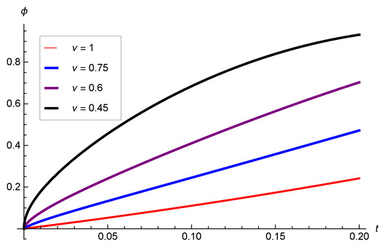
If we choose $\upsilon =1$, then Equation (23) becomes

$$\varphi \left(t\right)=1+\sqrt{2}tanh\left(\sqrt{2}t+\frac{1}{2}log\left(\frac{\sqrt{2}-1}{\sqrt{2}+1}\right)\right).$$

This exact solution agrees with the one appearing in the literature (see Figure 1 and Table 1).

Figure 1. These are solutions for example 1 for distinct values of υ.

Table 1. Numerical Values for example 1 for different values of υ, CT = 10 min.

t	$\mathit{\upsilon }=0.45$	$\mathit{\upsilon }=0.6$	$\mathit{\upsilon }=0.75$	$\mathit{\upsilon }$ = 1
				Numerical	Exact
$0.2$	$0.931788$	$0.702985$	$0.471891$	$0.241863$	$0.2419768$
0.4	$0.706152$	$1.02876$	$0.897507$	$0.564371$	$0.564371$
0.6	$-0.432075$	$0.794303$	$1.11755$	$0.926696$	$0.9535662$
0.8	$-2.4294$	$-0.222495$	$0.873956$	$1.2210187$	$1.3463637$
1	$-5.21527$	$-2.18641$	$-0.117103$	$1.2555556$	$1.6894984$

Example 2.

Let us consider one model of the time fractional diffusion as

$${}^c{D}_t^{\upsilon }\varphi (x,t)={\varphi }_{xx}(x,t)+\varphi (x,t),x,t>0,0<\upsilon \le 1,$$

(25)

together with initial condition

$$\varphi (x,0)=cos\left(\pi x\right).$$

(26)

Employ first Theorem 1 to Equation (24) to see that

$$\begin{array}{ccc}\hfill {\mathcal{N}}^{+}\left(\varphi (x,t)\right)& =& {\displaystyle \frac{u^{\upsilon }}{s^{\upsilon }}\sum _{k=0}^{n-1}\frac{s^{\upsilon -(k+1)}}{u^{\upsilon -k}}{D}_t^k\varphi (x,0)+\frac{u^{\upsilon }}{s^{\upsilon }}{\mathcal{N}}^{+}\left({\varphi }_{xx}\right)+\frac{u^{\upsilon }}{s^{\upsilon }}{\mathcal{N}}^{+}\left(\varphi \right)}\hfill \\ \\ \hfill & =& \frac{1}{s}\varphi (x,0)+\frac{u^{\upsilon }}{s^{\upsilon }}{\mathcal{N}}^{+}\left({\varphi }_{xx}\right)+\frac{u^{\upsilon }}{s^{\upsilon }}{\mathcal{N}}^{+}\left(\varphi \right).\hfill \end{array}$$

(27)

Taking the N-transform inverse of Equation (26), we arrive at

$$\varphi (x,t)=cos\left(\pi x\right)+{\mathcal{N}}^{-1}\left(\frac{u^{\upsilon }}{s^{\upsilon }}{\mathcal{N}}^{+}\left({\varphi }_{xx}\right)\right)+{\mathcal{N}}^{-1}\left(\frac{u^{\upsilon }}{s^{\upsilon }}{\mathcal{N}}^{+}\left(\varphi \right)\right).$$

(28)

Suppose that our solution for $\varphi (x,t)$ is

$$\varphi (x,t)=\sum _{n=0}^{\infty }{\varphi }_n(x,t).$$

(29)

One sees from Equations (27) and (28), that Equation (26) becomes

$$\sum _{n=0}^{\infty }{\varphi }_n(x,t)=cos\left(\pi x\right)+{\mathcal{N}}^{-1}\left(\frac{u^{\upsilon }}{s^{\upsilon }}{\mathcal{N}}^{+}\left(\sum _{n=0}^{\infty }{\varphi }_{nxx}(x,t)\right)\right)+{\mathcal{N}}^{-1}\left(\frac{u^{\upsilon }}{s^{\upsilon }}{\mathcal{N}}^{+}\left(\sum _{n=0}^{\infty }{\varphi }_n(x,t)\right)\right).$$

(30)

Looking at Equation (29), one can get

$$\begin{array}{c}{\varphi }_0(x,t)=cos\left(\pi x\right)\hfill \\ \\ {\varphi }_1(x,t)={\mathcal{N}}^{-1}\left(\frac{u^{\upsilon }}{s^{\upsilon }}{\mathcal{N}}^{+}\left({\varphi }_{0xx}\right)\right)+{\mathcal{N}}^{-1}\left(\frac{u^{\upsilon }}{s^{\upsilon }}{\mathcal{N}}^{+}\left({\varphi }_0\right)\right)\hfill \\ \\ {\varphi }_2(x,t)={\mathcal{N}}^{-1}\left(\frac{u^{\upsilon }}{s^{\upsilon }}{\mathcal{N}}^{+}\left({\varphi }_{1xx}\right)\right)+{\mathcal{N}}^{-1}\left(\frac{u^{\upsilon }}{s^{\upsilon }}{\mathcal{N}}^{+}\left({\varphi }_1\right)\right)\hfill \\ \\ {\varphi }_3(x,t)={\mathcal{N}}^{-1}\left(\frac{u^{\upsilon }}{s^{\upsilon }}{\mathcal{N}}^{+}\left({\varphi }_{2xx}\right)\right)+{\mathcal{N}}^{-1}\left(\frac{u^{\upsilon }}{s^{\upsilon }}{\mathcal{N}}^{+}\left({\varphi }_2\right)\right).\hfill \end{array}$$

We follow this direction to obtain

$${\varphi }_{n+1}(x,t)={\mathcal{N}}^{-1}\left(\frac{u^{\upsilon }}{s^{\upsilon }}{\mathcal{N}}^{+}\left({\varphi }_{nxx}\right)\right)+{\mathcal{N}}^{-1}\left(\frac{u^{\upsilon }}{s^{\upsilon }}{\mathcal{N}}^{+}\left({\varphi }_n\right)\right).$$

Finally, with the help of Equation (29), one can easily explore the rest of the iterations

$$\begin{array}{ccc}\hfill {\varphi }_1(x,t)& =& {\mathcal{N}}^{-1}\left(\frac{u^{\upsilon }}{s^{\upsilon }}{\mathcal{N}}^{+}\left({\varphi }_{0xx}\right)\right)+{\mathcal{N}}^{-1}\left(\frac{u^{\upsilon }}{s^{\upsilon }}{\mathcal{N}}^{+}\left({\varphi }_0\right)\right)\hfill \\ \\ \hfill & =& {\mathcal{N}}^{-1}\left(\frac{u^{\upsilon }}{s^{\upsilon }}{\mathcal{N}}^{+}\left(-{\pi }^{2}cos\left(\pi x\right)\right)\right)+{\mathcal{N}}^{-1}\left(\frac{u^{\upsilon }}{s^{\upsilon }}{\mathcal{N}}^{+}\left(cos\left(\pi x\right)\right)\right)\hfill \\ \\ \hfill & =& {\mathcal{N}}^{-1}\left(\frac{u^{\upsilon }}{s^{\upsilon }}\frac{-{\pi }^{2}cos\left(\pi x\right)}{s}\right)+{\mathcal{N}}^{-1}\left(\frac{u^{\upsilon }\pi cos\left(\pi x\right)}{s^{\upsilon +1}}\right)\hfill \\ \\ \hfill & =& \left(1-{\pi }^2\right)cos\left(\pi x\right)\frac{t^{\upsilon }}{\mathsf{\Gamma }\left(\upsilon +1\right)}.\hfill \end{array}$$

Likewise,

$$\begin{array}{c}{\varphi }_2(x,t)={\left(1-{\pi }^2\right)}^{2}cos\left(\pi x\right)\frac{t^{2\upsilon }}{\mathsf{\Gamma }\left(2\upsilon +1\right)}\hfill \\ \\ {\varphi }_3(x,t)={\left(1-{\pi }^2\right)}^{3}cos\left(\pi x\right)\frac{t^{3\upsilon }}{\mathsf{\Gamma }(3\upsilon +1)}.\hfill \end{array}$$

Our approximate solution for $\varphi (x,t)$ is now of the form

$$\begin{array}{cc}\hfill \varphi (x,t)& {\displaystyle =\sum _{n=0}^{\infty }{\varphi }_n\left(x,t\right)}\hfill \\ \hfill & ={\varphi }_0\left(x,t\right)+{\varphi }_1\left(x,t\right)+{\varphi }_2\left(x,t\right)+{\varphi }_3\left(x,t\right)+\dots \hfill \\ & =cos\left(\pi x\right)\left(1+\left(1-{\pi }^2\right)\frac{t^{\upsilon }}{\mathsf{\Gamma }\left(\upsilon +1\right)}+{\left(1-{\pi }^2\right)}^2\frac{t^{2\upsilon }}{\mathsf{\Gamma }\left(2\upsilon +1\right)}+{\left(1-{\pi }^2\right)}^3\frac{t^{3\upsilon }}{\mathsf{\Gamma }\left(3\upsilon +1\right)}+\dots \right)\hfill \end{array}$$

Therefore, our exact solution is

$$\varphi (x,t)=cos\left(\pi x\right)E_{\upsilon }\left(\left(1-{\pi }^2\right)t^{\upsilon }\right).$$

(31)

Substitute $\upsilon =1$ in Equation (30) to conclude

$$\varphi (x,t)=cos\left(\pi x\right)e^{\left(1-{\pi }^2\right)t}.$$

This is indeed the intended solution for Equation (24) which exists through out the literature (see Table 2).

Table 2. Numerical results for Example 2 for distinct values for υ, CT = 10 min.

x	t	$\mathit{\upsilon }=0.25$	$\mathit{\upsilon }=0.5$	$\mathit{\upsilon }=0.75$	$\mathit{\upsilon }$ = 1
					Numerical	Exact
0	0.02	0.20104552	0.36691625	0.61998793	0.83745132 0.83745132
	0.04	0.17414299	0.28187077	0.46534302	0.70132479 0.70132479
	0.06	0.15978832	0.23813296	0.37076063	0.58732540 0.58732540
	0.08	0.1502041	0.21016121	0.30658126	0.49185646 0.49185646
	0.1	0.14310464	0.19025412	0.26034611	0.41190586 0.41190586
1/4	0.02	0.14216065	0.25944897	0.43839767	0.59216754 0.59216754
	0.04	0.12313769	0.19931273	0.32904721	0.49591151 0.49591151
	0.06	0.11298741	0.16838543	0.26216736	0.41530177 0.41530177
	0.08	0.10621033	0.14860641	0.21678569	0.34779504 0.34779504
	0.1	0.10119026	0.13452998	0.1840925	0.29126143 0.29126143
1/3	0.02	0.10052276	0.18345812	0.30999396	0.41872568 0.41872568
	0.04	0.087071497	0.14093539	0.23267151	0.35066239 0.35066239
	0.06	0.079894162	0.11906648	0.18538032	0.29366270 0.29366270
	0.08	0.075102048	0.1050806	0.15329063	0.24592823 0.24592823
	0.1	0.071552321	0.09512706	0.13017306	0.20595293 0.20595293

Remark 2.

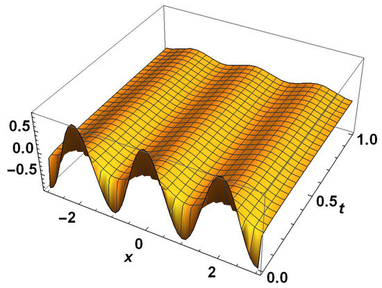
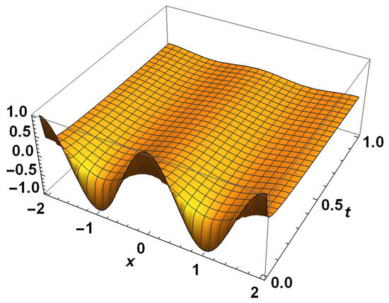
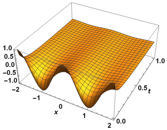
Figure 2, Figure 3, Figure 4 and Figure 5 show that the solution peak is high, and one can see that the peak of the solutions of the diffusion equation becomes more and more smooth as the fractional factor υ increases.

Figure 2. Exact solutions for example 2 with $\upsilon =0.25$.

Figure 3. Exact solutions for example 2 with $\upsilon =0.5$.

Figure 4. Exact solutions for example 2 with $\upsilon =0.75$.

Figure 5. Exact solutions for example 2 with $\upsilon =1$.

4. Fractional Systems of Ordinary Differential Equations

Next, let us examine two models of systems of FDEs. Then, we present numerical values in tables for some values of t. We only used 5th order approximate solutions for the two functions.

Example 3.

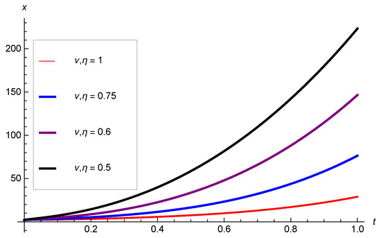
Given the system of LFDE in the form (see Figure 6 and Figure 7 and Table 3)

$$\begin{array}{c}{}^c{D}_t^{\upsilon }x\left(t\right)=2x\left(t\right)+y\left(t\right),0<\upsilon \le 1\hfill \\ \\ {}^c{D}_t^{\eta }y\left(t\right)=x\left(t\right)+2y\left(t\right),0<\eta \le 1\hfill \end{array}$$

(32)

together with value conditions

$$x\left(0\right)=2,y\left(0\right)=1.$$

(33)

Figure 6. Approximate solutions $x\left(t\right)$ for example 3 with some values of $\upsilon ,\eta$.

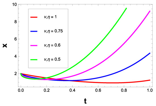
Figure 7. Approximate solutions $y\left(t\right)$ for example 3 with some values of $\upsilon ,\eta$.

Table 3. The numerical values for $x\left(t\right)$ with some values for υ and η, CT = 10 min.

t	$\mathit{\upsilon }=\mathit{\eta }=0.5$	$\mathit{\upsilon }=\mathit{\eta }=0.6$	$\mathit{\upsilon }=\mathit{\eta }=0.75$	$\mathit{\upsilon }$ = 1
				Numerical	Exact
$0.2$	$14.4864$	$8.66865$	$5.21454$	$3.04352$	$3.04352$
0.4	$39.8447$	$22.5925$	$11.4568$	$4.81194$	$4.81194$
0.6	$81.6907$	$47.9029$	$23.3317$	$7.87177$	$7.87177$
0.8	$142.225$	$88.083192$	$43.831967$	$13.2487$	$13.2487$
1	$223.31317$	$146.51415$	$76.394554$	$22.8038$	$22.8038$

Applying the natural transform of Equations (32) and (33), one concludes

$$\begin{array}{c}{\mathcal{N}}^{+}\left(x\left(t\right)\right)=\frac{2}{s}+2\frac{u^{\upsilon }}{s^{\upsilon }}{\mathcal{N}}^{+}\left(x\left(t\right)\right)+\frac{u^{\upsilon }}{s^{\upsilon }}{\mathcal{N}}^{+}\left(y\left(t\right)\right)\hfill \\ \\ {\mathcal{N}}^{+}\left(y\left(t\right)\right)=\frac{1}{s}+\frac{u^{\eta }}{s^{\eta }}{\mathcal{N}}^{+}\left(x\left(t\right)\right)+2\frac{u^{\eta }}{s^{\eta }}{\mathcal{N}}^{+}\left(y\left(t\right)\right).\hfill \end{array}$$

(34)

Using the ${\mathcal{N}}^{-1}$ on Equation (34) we arrive at

$$\begin{array}{c}x\left(t\right)=2+2{\mathcal{N}}^{-1}\left(\frac{u^{\upsilon }}{s^{\upsilon }}{\mathcal{N}}^{+}\left(x\left(t\right)\right)\right)+{\mathcal{N}}^{-1}\left(\frac{u^{\upsilon }}{s^{\upsilon }}{\mathcal{N}}^{+}\left(y\left(t\right)\right)\right)\hfill \\ \\ y\left(t\right)=1+{\mathcal{N}}^{-1}\left(\frac{u^{\eta }}{s^{\eta }}{\mathcal{N}}^{+}\left(x\left(t\right)\right)\right)+2{\mathcal{N}}^{-1}\left(\frac{u^{\eta }}{s^{\eta }}{\mathcal{N}}^{+}\left(y\left(t\right)\right)\right).\hfill \end{array}$$

(35)

Suppose our solutions are of the forms

$$x\left(t\right)=\sum _{n=0}^{\infty }{x}_n\left(t\right),y\left(t\right)=\sum _{n=0}^{\infty }{y}_n\left(t\right).$$

(36)

Then we get,

$$\begin{array}{c}{\displaystyle \sum _{n=0}^{\infty }{x}_n\left(t\right)=2+2{\mathcal{N}}^{-1}\left(\frac{u^{\upsilon }}{s^{\upsilon }}{\mathcal{N}}^{+}\left(x\left(t\right)\right)\right)+{\mathcal{N}}^{-1}\left(\frac{u^{\upsilon }}{s^{\upsilon }}{\mathcal{N}}^{+}\left(y\left(t\right)\right)\right)}\hfill \\ \\ {\displaystyle \sum _{n=0}^{\infty }{y}_n\left(t\right)=1+{\mathcal{N}}^{-1}\left(\frac{u^{\eta }}{s^{\eta }}{\mathcal{N}}^{+}\left(x\left(t\right)\right)\right)+2{\mathcal{N}}^{-1}\left(\frac{u^{\eta }}{s^{\eta }}{\mathcal{N}}^{+}\left(y\left(t\right)\right)\right)}.\hfill \end{array}$$

(37)

Using Equation (37) we obtain

$$x_0\left(0\right)=2,y_0\left(0\right)=1$$

$$\begin{array}{c}{x}_1\left(t\right)=2{\mathcal{N}}^{-1}\left(\frac{u^{\upsilon }}{s^{\upsilon }}{\mathcal{N}}^{+}\left(x_0\left(t\right)\right)\right)+{\mathcal{N}}^{-1}\left(\frac{u^{\upsilon }}{s^{\upsilon }}{\mathcal{N}}^{+}\left(y_0\left(t\right)\right)\right)=\frac{5t^{\upsilon }}{\mathsf{\Gamma }\left(\upsilon +1\right)}\hfill \\ \\ y_1\left(t\right)=-{\mathcal{N}}^{-1}\left(\frac{u^{{}^{\eta }}}{s^{{}^{\eta }}}{\mathcal{N}}^{+}\left(x_0\left(t\right)\right)\right)+{\mathcal{N}}^{-1}\left(\frac{u^{\eta }}{s^{{}^{\eta }}}{\mathcal{N}}^{+}\left(y_0\left(t\right)\right)\right)=\frac{4t^{\eta }}{\mathsf{\Gamma }\left(\eta +1\right)}.\hfill \end{array}$$

Likewise,

$$\begin{array}{c}{x}_2\left(t\right)=\frac{10t^{2\upsilon }}{\mathsf{\Gamma }\left(2\upsilon +1\right)}+\frac{4t^{\upsilon +\eta }}{\mathsf{\Gamma }\left(\upsilon +\eta +1\right)}\hfill \\ \\ y_2\left(t\right)=\frac{8t^{2\eta }}{\mathsf{\Gamma }\left(2\eta +1\right)}+\frac{5t^{\upsilon +\eta }}{\mathsf{\Gamma }\left(\upsilon +\eta +1\right)}.\hfill \end{array}$$

We proceed in a similar way to get

$$\begin{array}{c}{x}_3\left(t\right)=\frac{20}{\mathsf{\Gamma }\left(3\upsilon +1\right)}{t}^{3\upsilon }+\frac{13}{\mathsf{\Gamma }\left(2\upsilon +\eta +1\right)}{t}^{2\upsilon +\eta }+\frac{8}{\mathsf{\Gamma }\left(\alpha +2\eta +1\right)}{t}^{\upsilon +2\eta }\hfill \\ \\ y_3\left(t\right)=\frac{16}{\mathsf{\Gamma }\left(3\eta +1\right)}{t}^{3\eta }+\frac{28}{\mathsf{\Gamma }\left(\upsilon +2\eta +1\right)}{t}^{\upsilon +2\eta }+\frac{10}{\mathsf{\Gamma }\left(2\upsilon +\eta +1\right)}{t}^{2\upsilon +\eta }.\hfill \end{array}$$

$$\begin{array}{c}{x}_4\left(t\right)=\frac{40}{\mathsf{\Gamma }\left(4\upsilon +1\right)}{t}^{4\upsilon }+\frac{36}{\mathsf{\Gamma }\left(3\upsilon +\eta +1\right)}{t}^{3\upsilon +\eta }+\frac{30}{\mathsf{\Gamma }\left(3\upsilon +2\eta +1\right)}{t}^{2\upsilon +2\eta }+\frac{16}{\mathsf{\Gamma }\left(\upsilon +3\eta +1\right)}{t}^{\upsilon +3\eta }\hfill \\ \\ y_4\left(t\right)=\frac{32}{\mathsf{\Gamma }\left(4\eta +1\right)}{t}^{4\eta }+\frac{36}{\mathsf{\Gamma }\left(\upsilon +3\eta +1\right)}{t}^{\upsilon +3\eta }+\frac{33}{\mathsf{\Gamma }\left(2\upsilon +2\eta +1\right)}{t}^{2\upsilon +2\eta }+\frac{20}{\mathsf{\Gamma }\left(3\upsilon +\eta +1\right)}{t}^{3\upsilon +\eta }\hfill \end{array}$$

Finally, the approximate solutions for these functions are

$$\begin{array}{ccc}\hfill x\left(t\right)& =& {\displaystyle \sum _{n=0}^{\infty }{x}_n\left(t\right)}\hfill \end{array}$$

$$\begin{array}{ccc}\hfill y\left(t\right)& =& {\displaystyle \sum _{n=0}^{\infty }{y}_n\left(t\right)}\hfill \end{array}.$$

Thus,

$$\begin{array}{c}x\left(t\right)=2+\frac{5t^{\upsilon }}{\mathsf{\Gamma }\left(\upsilon +1\right)}+\frac{10t^{2\upsilon }}{\mathsf{\Gamma }\left(2\upsilon +1\right)}+\frac{4t^{\upsilon +\eta }}{\mathsf{\Gamma }\left(\upsilon +\eta +1\right)}+\frac{20t^{3\upsilon }}{\mathsf{\Gamma }\left(3\upsilon +1\right)}+\frac{8t^{\upsilon +2\eta }}{\mathsf{\Gamma }\left(\upsilon +2\eta +1\right)}+\frac{13t^{2\upsilon +\eta }}{\mathsf{\Gamma }\left(2\upsilon +\eta +1\right)}+\dots \hfill \\ \\ y\left(t\right)=1+\frac{4t^{\eta }}{\mathsf{\Gamma }\left(\eta +1\right)}+\frac{8t^{2\eta }}{\mathsf{\Gamma }\left(2\eta +1\right)}+\frac{5t^{\upsilon +\eta }}{\mathsf{\Gamma }\left(\upsilon +\eta +1\right)}+\frac{16t^{3\eta }}{\mathsf{\Gamma }\left(3\eta +1\right)}+\frac{14t^{\upsilon +2\eta }}{\mathsf{\Gamma }\left(\upsilon +2\eta +1\right)}+\frac{10t^{2\upsilon +\eta }}{\mathsf{\Gamma }\left(2\upsilon +\eta +1\right)}+\dots \hfill \end{array}$$

Note that when $\upsilon =\eta =1$, then the exact solutions are

$$x\left(t\right)=e^t+e^{3t};y\left(t\right)=-e^t+e^{3t}.$$

Example 4.

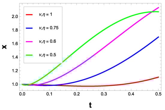
Suppose we are given a system of LFDE (see Figure 8 and Figure 9 and Table 4)

$$\begin{array}{c}{}^c{D}_t^{\upsilon }x\left(t\right)=y\left(t\right)-2x\left(t\right),0<\upsilon \le 1\hfill \\ \\ {}^c{D}_t^{\eta }y\left(t\right)=x\left(t\right)-2y\left(t\right),0<\eta \le 1\hfill \end{array}$$

(38)

together with two value conditions

$$x\left(0\right)=2,y\left(0\right)=1.$$

(39)

Figure 8. Approximate solutions $x\left(t\right)$ for Example 4 with some values of $\upsilon ,\eta$.

Figure 9. Approximate solutions $y\left(t\right)$ for Example 4 with some values of $\upsilon ,\eta$.

Table 4. The results obtained for $x\left(t\right)$ with different values of υ and η, CT = 10 min.

t	$\mathit{\upsilon }=\mathit{\eta }=0.5$	$\mathit{\upsilon }=\mathit{\eta }=0.6$	$\mathit{\upsilon }=\mathit{\eta }=0.75$	$\mathit{\upsilon }=\mathit{\eta }$ = 1
				Numerical	Exact
$0.2$	$14.4864$	$8.66865$	$5.21454$	$1.36754$	$1.36754$
0.4	$39.8447$	$22.5925$	$11.4568$	$0.971514$	$0.971514$
0.6	$81.6907$	$47.9029$	$23.3317$	$0.714111$	$0.714111$
0.8	$142.225$	$88.083192$	$43.831967$	$0.540047$	$0.540047$
1	$223.31317$	$146.51415$	$76.394554$	$0.417667$	$0.417667$

Apply natural transform to Equations (38) and (39), to get

$$\begin{array}{c}{\mathcal{N}}^{+}\left(x\left(t\right)\right)=\frac{2}{s}+\frac{u^{\upsilon }}{s^{\upsilon }}{\mathcal{N}}^{+}\left(y\left(t\right)\right)-2\frac{u^{\upsilon }}{s^{\upsilon }}{\mathcal{N}}^{+}\left(x\left(t\right)\right)\hfill \\ \\ {\mathcal{N}}^{+}\left(y\left(t\right)\right)=\frac{1}{s}+\frac{u^{\eta }}{s^{\eta }}{\mathcal{N}}^{+}\left(y\left(t\right)\right)-2\frac{u^{\eta }}{s^{\eta }}{\mathcal{N}}^{+}\left(x\left(t\right)\right).\hfill \end{array}$$

(40)

Moreover, applying ${\mathcal{N}}^{-1}$ on Equation (40)

$$\begin{array}{c}x\left(t\right)=2+{\mathcal{N}}^{-1}\left[\frac{u^{\upsilon }}{s^{\upsilon }}{\mathcal{N}}^{+}\left(y\left(t\right)\right)\right]-2{\mathcal{N}}^{-1}\left[\frac{u^{\upsilon }}{s^{\upsilon }}{\mathcal{N}}^{+}\left(x\left(t\right)\right)\right]\hfill \\ \\ y\left(t\right)=1+{\mathcal{N}}^{-1}\left[\frac{u^{\eta }}{s^{\eta }}{\mathcal{N}}^{+}\left(x\left(t\right)\right)\right]-2{\mathcal{N}}^{-1}\left[\frac{u^{\eta }}{s^{\eta }}{\mathcal{N}}^{+}\left(y\left(t\right)\right)\right].\hfill \end{array}$$

(41)

Suppose our approximate solutions are given as

$$x\left(t\right)=\sum _{n=0}^{\infty }{x}_n\left(t\right);y\left(t\right)=\sum _{n=0}^{\infty }{y}_n\left(t\right).$$

(42)

Using Equation (42), then Equation (41) becomes

$$\begin{array}{c}{\displaystyle \sum _{n=0}^{\infty }{x}_n\left(t\right)=2+{\mathcal{N}}^{-1}\left(\frac{u^{\upsilon }}{s^{\upsilon }}{\mathcal{N}}^{+}\left(y_n\left(t\right)\right)\right)-2{\mathcal{N}}^{-1}\left(\frac{u^{\upsilon }}{s^{\upsilon }}{\mathcal{N}}^{+}\left(x_n\left(t\right)\right)\right)}\hfill \\ \\ {\displaystyle \sum _{n=0}^{\infty }{y}_n\left(t\right)=1+{\mathcal{N}}^{-1}\left(\frac{u^{\eta }}{s^{\eta }}{\mathcal{N}}^{+}\left(x_n\left(t\right)\right)\right)-2{\mathcal{N}}^{-1}\left(\frac{u^{\eta }}{s^{\eta }}{\mathcal{N}}^{+}\left(y_n\left(t\right)\right)\right)}.\hfill \end{array}$$

(43)

One concludes from Equation (43)

$$x_0\left(0\right)=2,y_0\left(0\right)=1$$

$$\begin{array}{c}{x}_1\left(t\right)={\mathcal{N}}^{-1}\left(\frac{u^{\upsilon }}{s^{\upsilon }}{\mathcal{N}}^{+}\left(y_0\left(t\right)\right)\right)-2{\mathcal{N}}^{-1}\left(\frac{u^{\upsilon }}{s^{\upsilon }}{\mathcal{N}}^{+}\left(x_0\left(t\right)\right)\right)=\frac{-3t^{\upsilon }}{\mathsf{\Gamma }\left(\upsilon +1\right)}\hfill \\ \\ y_1\left(t\right)={\mathcal{N}}^{-1}\left(\frac{u^{\eta }}{s^{\eta }}{\mathcal{N}}^{+}\left(x_0\left(t\right)\right)\right)-2{\mathcal{N}}^{-1}\left(\frac{u^{\eta }}{s^{\eta }}{\mathcal{N}}^{+}\left(y_0\left(t\right)\right)\right)=0.\hfill \end{array}$$

Likewise,

$$\begin{array}{c}{x}_2\left(t\right)=\frac{6t^{2\upsilon }}{\mathsf{\Gamma }\left(2\upsilon +1\right)}\hfill \\ \\ y_2\left(t\right)=\frac{-3t^{\upsilon +\eta }}{\mathsf{\Gamma }\left(\upsilon +\eta +1\right)}.\hfill \end{array}$$

We proceed as before to obtain

$$\begin{array}{c}{x}_3\left(t\right)=\frac{-3t^{2\upsilon +\eta }}{\mathsf{\Gamma }\left(2\upsilon +\eta +1\right)}-\frac{12t^{3\upsilon }}{\mathsf{\Gamma }\left(3\upsilon +1\right)}\hfill \\ \\ y_3\left(t\right)=\frac{12t^{\upsilon +2\eta }}{\mathsf{\Gamma }\left(\upsilon +2\eta +1\right)}+\frac{6t^{2\upsilon +\eta }}{\mathsf{\Gamma }\left(2\upsilon +\eta +1\right)}\hfill \end{array}$$

$$\begin{array}{c}{x}_4\left(t\right)=\frac{24t^{4\upsilon }}{\mathsf{\Gamma }\left(4\upsilon +1\right)}+\frac{12t^{3\upsilon +\eta }}{\mathsf{\Gamma }\left(3\upsilon +\eta +1\right)}+\frac{6t^{2\upsilon +2\eta }}{\mathsf{\Gamma }\left(2\upsilon +2\beta +1\right)}\hfill \\ \\ y_4\left(t\right)=\frac{-12t^{\upsilon +3\eta }}{\mathsf{\Gamma }\left(\upsilon +3\eta +1\right)}-\frac{15t^{2\upsilon +2\eta }}{\mathsf{\Gamma }\left(2\upsilon +2\eta +1\right)}-\frac{12t^{3\upsilon +\eta }}{\mathsf{\Gamma }\left(3\upsilon +\eta +1\right)}.\hfill \end{array}$$

Finally, the approximate solutions for these functions are as follows

$$x\left(t\right)=\sum _{n=0}^{\infty }{x}_n\left(t\right);y\left(t\right)=\sum _{n=0}^{\infty }{y}_n\left(t\right).$$

(44)

It follows that,

$$\begin{array}{c}x\left(t\right)=2-\frac{3t^{\upsilon }}{\mathsf{\Gamma }\left(\upsilon +1\right)}+\frac{6t^{2\upsilon }}{\mathsf{\Gamma }\left(2\upsilon +1\right)}-\frac{3t^{2\upsilon +\eta }}{\mathsf{\Gamma }\left(2\upsilon +\eta +1\right)}-\frac{3t^{3\upsilon }}{\mathsf{\Gamma }\left(3\upsilon +1\right)}+\frac{6t^{2\upsilon +2\eta }}{\mathsf{\Gamma }\left(2\upsilon +2\eta +1\right)}+\frac{12t^{3\upsilon +\eta }}{\mathsf{\Gamma }\left(3\upsilon +\eta +1\right)}+\frac{24t^{4\upsilon }}{\mathsf{\Gamma }\left(4\upsilon +1\right)}\dots \hfill \\ \\ y\left(t\right)=1-\frac{3t^{\upsilon +\eta }}{\mathsf{\Gamma }\left(\upsilon +\eta +1\right)}+\frac{6t^{\upsilon +2\eta }}{\mathsf{\Gamma }\left(\upsilon +2\eta +1\right)}+\frac{6t^{2\upsilon +\eta }}{\mathsf{\Gamma }\left(2\upsilon +\eta +1\right)}-\frac{15t^{2\upsilon +2\eta }}{\mathsf{\Gamma }\left(2\upsilon +2\eta +1\right)}-\frac{12t^{3\upsilon +\eta }}{\mathsf{\Gamma }\left(3\upsilon +\eta +1\right)}-\frac{12t^{\upsilon +2\eta }}{\mathsf{\Gamma }\left(\upsilon +2\eta +1\right)},\dots .\hfill \end{array}$$

Note that when $\upsilon =\eta =1$, then the exact solutions are

$$x\left(t\right)=e^{-3t}+e^{-t};y\left(t\right)=e^{-3t}-e^{-t}.$$

5. Discussion and Conclusions

Many techniques were used, prior to this work, to handle FDEs. In this work, we have implemented an efficient integral transform method called the Fractional Decomposition Method (FDM) and given detailed proofs to some theorems using the proposed method. We have successfully employed the FDM to obtain exact solutions for the diffusion fractional differential equation and analytical solutions for nonlinear fractional ODE including approximate solutions to two systems of fractional ODE. The FDM reduces the computational difficulties currently exist in the literature. The FDM has self-efficient properties, which help in solving some application with fractional derivatives problems. Our numerical results show that the FDM is a valid and easy scheme for obtaining exact and approximate solutions to fractional differential equation problems. It is proven that the FDM can be implemented without discretization, linearization and perturbation methods used in solving fractional differential equation applications. Thus, it is considered as another option to existing schemes and can be used for wide applications. The FDM has been implemented to many linear and nonlinear FDEs and we have not faced any difficulties when using the new mechanism. Our aim, in the future, is to explore more properties to help solve applications of the FDM, test reasonable series, which converge very fast, and employ it to other fractional integral equation applications.

Finally, the numerical results showed that the new scheme is accurate and efficient. We were able to explore solutions to physical models when $\upsilon =\eta =1$. The next step for our research is to further apply the new scheme to other FDEs that arise in other areas of scientific fields. Earlier works [4,6,14,21] have developed efficient techniques but specialized only for usage on solving specific type of problems, but our FNDM expands their applicability since it is so general.

References

- Roberts, M. Signals and Systems: Analysis Using Transform Methods and Matlab, 2nd ed.; McGraw-Hill: New York, NY, USA, 2003. [Google Scholar]
- Ortigueira, M.D.; Valério, D. Fractional Signals and Systems; Walter de Gruyter GmbH & Co KG: Berlin, Germany, 2020. [Google Scholar]
- Nigmatullin, R.R. To the theoretical explanation of the “universal response”. Phys. Status Solidi B 1984, 123, 739–745. [Google Scholar] [CrossRef]
- Coussot, C.; Kalyanam, S.; Yapp, R.; Insana, M.F. Fractional derivative models for ultrasonic characterization of polymer and breast tissue viscoelasticity. IEEE Trans. Ultrason. Ferroelectr. Freq. Control 2009, 56, 715–726. [Google Scholar] [CrossRef] [PubMed]
- Noeiaghdam, S.; Sidorov, D. Caputo-Fabrizio fractional derivative to solve the fractional model of energy supply-demand system. Math. Model. Eng. Probl. 2020, 7, 359–367. [Google Scholar] [CrossRef]
- Djordjević, V.D.; Jarić, J.; Fabry, B.; Fredberg, J.J.; Stamenović, D. Fractional derivatives embody essential features of cell rheological behavior. Ann. Biomed. Eng. 2003, 31, 692–699. [Google Scholar] [CrossRef] [PubMed]
- Noeiaghdam, S.; Sidorov, D.; Wazwaz, A.M.; Sidorov, N.; Sizikov, V. The Numerical Validation of the Adomian Decomposition Method for Solving Volterra Integral Equation with Discontinuous Kernels Using the CESTAC Method. Mathematics 2021, 9, 260. [Google Scholar] [CrossRef]
- Adomian, G. A new approach to nonlinear partial differential equations. J. Math. Anal. Appl. 1984, 102, 420–434. [Google Scholar] [CrossRef]
- Ghosh, U.; Sarkar, S.; Das, S. Solution of system of linear fractional differential equations with modified derivative of Jumarie type. arXiv 2015, arXiv:1510.00385. [Google Scholar]
- Guo, S.; Mei, L.; Li, Y.; Sun, Y. The improved fractional sub-equation method and its applications to the space–time fractional differential equations in fluid mechanics. Phys. Lett. A 2012, 376, 407–411. [Google Scholar] [CrossRef]
- Argyros, I.K. Iterative Methods and Their Dynamics with Applications: A Contemporary Study; CRC Press: Boca Raton, FL, USA, 2017. [Google Scholar]
- Anastassiou, G.A.; Argyros, I.K. Intelligent Numerical Methods: Applications to Fractional Calculus; Springer International Publishing: Berlin/Heidelberg, Germany, 2016. [Google Scholar]
- Samko, S.G.; Kilbas, A.A.; Marichev, O.I. Fractional Integrals and Derivatives; Translated from the 1987 Russian Original; Gordon and Breach Science Publishers: New York, NY, USA, 1987. [Google Scholar]
- Podlubny, I. Fractional Differential Equations; Academic Press: San Diego, CA, USA, 1999. [Google Scholar]
- Jian, S.; Zhang, J.; Zhang, Q.; Zhang, Z. Fast evaluation of the Caputo fractional derivative and its applications to fractional diffusion equations. Commun. Comput. Phys. 2017, 21, 650–678. [Google Scholar] [CrossRef]
- Gu, X.-M.; Wu, S.-L. A parallel-in-time iterative algorithm for Volterra partial integro-differential problems with the weakly singular kernel. J. Comput. Phys. 2020, 13, 109576. [Google Scholar] [CrossRef]
- Mainardi, F. Fractional calculus. In Fractals and Fractional Calculus in Continuum Mechanics; Springer: Vienna, Austria, 1997. [Google Scholar]
- Sevimlican, A. An approximation to solution of space and time fractional telegraph equations by He’s variational iteration method. Math. Probl. Eng. 2010, 2010, 290631. [Google Scholar] [CrossRef]
- Hu, Y.; Luo, Y.; Lu, Z. Analytical solution of the linear fractional differential equation by Adomian decomposition method. J. Comput. Appl. Math. 2008, 215, 220–229. [Google Scholar] [CrossRef]
- Liu, Y.; Du, Y.; Li, H.; He, S.; Gao, W. Finite difference/finite element method for a nonlinear time-fractional fourth-order reaction–diffusion problem. Comput. Math. Appl. 2015, 70, 573–591. [Google Scholar] [CrossRef]
- Rybakov, K.; Yushchenko, A. Spectral method for solving linear Caputo fractional stochastic differential equations. In IOP Conference Series: Materials Science and Engineering; IOP Publishing: Bristol, UK, 2020; Volume 1, p. 012077. [Google Scholar]
- Li, Z.B.; He, J.H. Fractional complex transform for fractional differential equations. Math. Comput. Appl. 2010, 15, 970–973. [Google Scholar] [CrossRef]
- Ortigueira, M.D.; Machado, J.T. Revisiting the 1D and 2D Laplace transforms. Mathematics 2020, 8, 1330. [Google Scholar] [CrossRef]
- Momani, S.; Shawagfeh, N. Decomposition method for solving fractional Riccati differential equations. Appl. Math. Comput. 2006, 182, 1083–1092. [Google Scholar] [CrossRef]
- Eltayeb, H.; Abdalla, Y.T.; Bachar, I.; Khabir, M.H. Fractional telegraph equation and its solution by natural transform decomposition method. Symmetry 2019, 11, 334. [Google Scholar] [CrossRef]
- Belgacem, F.B.; Silambarasan, R. Maxwell’s equations by means of the natural transform. Math. Eng. Sci. Aerosp. 2012, 3, 313–323. [Google Scholar]
- Mittag–Leffler, G.M. Sur la Nouvelle Fonction Sur la Nouvelle Fonction; Eα (x), Comptes Rendus de l Académie des Sciences: Paris, France, 1903; pp. 554–558. [Google Scholar]
- Gorenflo, R.; Kilbas, A.A.; Mainardi, F.; Rogosin, S.V. Mittag–Leffler Functions, Related Topics and Applications; Springer: Berlin, Germeny, 2014. [Google Scholar]
Publisher’s Note: MDPI stays neutral with regard to jurisdictional claims in published maps and institutional affiliations. |
© 2021 by the authors. Licensee MDPI, Basel, Switzerland. This article is an open access article distributed under the terms and conditions of the Creative Commons Attribution (CC BY) license (https://creativecommons.org/licenses/by/4.0/).