Abstract
The redefined vacuum approach, which is frequently employed in the many-body perturbation theory, proved to be a powerful tool for formula derivation. Here, we elaborate this approach within the bound-state QED perturbation theory. In addition to general formulation, we consider the particular example of a single particle (electron or vacancy) excitation with respect to the redefined vacuum. Starting with simple one-electron QED diagrams, we deduce first- and second-order many-electron contributions: screened self-energy, screened vacuum polarization, one-photon exchange, and two-photon exchange. The redefined vacuum approach provides a straightforward and streamlined derivation and facilitates its application to any electronic configuration. Moreover, based on the gauge invariance of the one-electron diagrams, we can identify various gauge-invariant subsets within derived many-electron QED contributions.
1. Introduction
Highly charged ions are considered as one of the best available natural laboratories to access strong field effects at the moment; highlighting the need to go beyond the perturbative regime since for high Z, the expansion parameter is comparable to one (where Z is the nuclear charge number and is the fine-structure constant). Hence, calculations to all orders in are sought, which requires special methods of the bound-state quantum electrodynamics (QED) to be developed within the corresponding framework, known as the Furry picture [1]. Moreover, by pushing QED, in the presence of the binding nuclear field, to its limits is a great way to earn in-depth knowledge about the theory and to probe potential new physics [2]. Evaluation of the dynamical properties and the structure of highly relativistic, tightly bound electrons in highly charged ions with utmost accuracy represents one of the most important and demanding problems in modern theoretical atomic physics. Although many approximate methods have access to higher-order corrections within the Breit approximation, such as relativistic many-body perturbation theory (RMBPT), relativistic configuration–interaction (CI) method, or multi-configuration Dirac–Fock (MCDF) method, the increasing precision in modern spectroscopy enforces accurate ab initio description of few- to many-electron systems within the bound-state QED.
In general, QED can be applied to any many-electron atoms even though it is most deeply developed for hydrogen and helium [3], and hydrogen-like ions [4], where the accuracy of the calculations has reached a remarkably high level. In the case of hydrogen, highly accurate theoretical calculations being combined with experimental transition energies allowed one not only to probe QED but also to determine the Rydberg constant and the proton charge radius [5]. However, the independent measurement of the – transition in muonic hydrogen [6,7] reported a different value of the proton charge radius, which evoked the so-called “proton radius puzzle”. For the current status of this problem we refer the reader to [8]. The recent theoretical [9,10,11] and experimental [12,13] progress in the helium spectroscopy pushes forward the idea of the independent determination of the fine structure constant from low-Z QED [14,15]. In the case of highly charged ions, the comparison of the experimental value of the Lamb shift, eV [16], allows one to test the first-order QED effects on a level of 1.7% [17]. However, the probe of the second-order QED effects, which contribute eV [18], is limited by the experimental accuracy, where improvements represent a rather challenging task [19]. A way to reach a better comparison is to investigate the transition energies in many-electron ions, which spread from soft x-ray to ultraviolet and, therefore, are accessible by laser spectroscopy techniques over a wide range of Z values [20]. The question arises: can we perform ab initio QED calculations for many-electron systems? The second-order contributions in are evaluated only within the state-of-the-art QED calculations for helium-like [21,22,23,24,25,26], lithium-like [27,28,29,30], beryllium-like [31,32,33], boron-like [34,35,36], and sodium-like [37] ions. The computations are so far limited to such selected, relatively simple systems not only due to the complexity of numerical calculations but also because of difficulties in deriving formal expressions.
The concept of a vacuum redefinition naturally arose in quantum field theory due to the notion of the fully occupied negative-energy continuum of fermion states, the so-called Dirac sea. The vacuum redefinition technique is widely accepted and demonstrated within the relativistic many-body perturbation theory (RMBPT) formalism [38,39,40,41]. Since rigorous bound-state QED calculations for many-electron systems are not up-to-date, the corresponding application examples of this concept are difficult to source. In Reference [42], the authors considered the case of one electron over the closed shells in the context of the two-time Green’s function method developed in that work. In Reference [37], the problem of the rigorous QED formulation for many-electron systems within the S-matrix approach was considered and the usefulness of the vacuum redefinition by analogy with RMBPT was emphasized. In this work, we further elaborate the redefined vacuum approach within the QED perturbation theory. The essential notion in introducing a redefined vacuum is to separate the electron dynamics into the “core” and “valence” parts. The first part is relegated to the reference vacuum energy and can be neglected, e.g., when the transition energy is considered. This is formulated via a new Fermi level , which lies above all core electron states. The many-electron contributions are extracted as the difference of two integrals over altering integration contours, each in link with its respective vacuum state. In this way, the interaction of the reference particle (electron or hole) with core electrons is taken into account within the QED framework. The great advantage of the method is that instead of the all-electron states one deals with the few-valence-electron states, which represent a much smaller Hilbert space.
Furthermore, as we demonstrate, the method allows us to identify various gauge-invariant subsets of diagrams, which provides an efficient control on derived formulas and their numerical implementation.
Following the motivation outlined above, in our recent paper [43], we have derived the two-photon-exchange contribution within the redefined vacuum QED approach for the case of an atom with a single electron above closed shells. The current work aims to formulate the redefined vacuum approach within the rigorous bound-state QED framework for an arbitrary state. Final expressions for one- and two-particle states are presented. In order to illustrate the developed method, the first- (one-photon exchange) and second-order (screened QED and two-photon exchange) many-electron QED diagrams are derived for the case of single-vacancy atoms. Such an example is chosen due to the fact that two-photon-exchange correction is still uncalculated for fluorine-like ions [44,45,46] as well as due to recent experimental efforts for such systems [47,48].
The paper is organized as follows. Section 2 introduces the working framework, the concept of vacuum redefinition, and the summary of necessary tools. Based on the two-time Green’s function approach [42,49], the QED perturbation theory is formulated in Section 3. In particular, the general expressions are derived for one- and two-particle states on top of the redefined vacuum. In Section 4, applications of the formalism are delivered for first- and second-order QED diagrams. Section 5 includes the discussion of the obtained results and the conclusion. Moreover, in Appendix A and Appendix B, the complete sets of formulas are provided for the screened QED and two-photon exchange diagrams, respectively. A comparison between QED and RMBPT results for the two-photon exchange is included in Appendix C.
Natural units () are used throughout this paper, the fine structure constant is defined as . The metric tensor is taken to be . Unless explicitly stated, all integrals are meant to be on the interval .
2. General Formulation and Method
The one-particle states of the electron–positron field in the presence of external potential are described by the Dirac equation
where is the static solution and j uniquely characterizes the solution, i.e., stands for all quantum numbers. The corresponding time-dependent solution is multiplied by phase. and are Dirac matrices. The Furry picture [1] allows one to consider the eigenstates as the solutions of the Dirac equation in presence of an external classical field. In the original Furry picture, the potential considered is the Coulomb potential of the nucleus . The extended Furry picture incorporates some screening potential in addition to the Coulomb one, i.e., . The unperturbed normal-ordered Hamiltonian is given by [50]
where the fermion field operator is expanded in terms of creation and annihilation operators
where ( is the electron (positron) annihilation operator for an electron (positron) in the state j and () is the electron (positron) creation operator for an electron (positron) in the state j, fulfilling the usual anti-commutations relations. The Fermi level is usually set to separating the Dirac sea from the rest of the spectrum. Here and in what follows the RMBPT notations of Lindgren and Morisson [38] and Johnson [41] are used: v and h designate the valence electron and the hole state, respectively, stand for core orbitals, and correspond to any arbitrary states.
The concept of vacuum redefinition is exacerbated when the interest is focused on the transitions with a significant many-electron background remaining unchanged. The key feature is that the contributions, arising from the interaction between core electrons are canceled in the difference between the excited and the ground state energies, are not considered from the very beginning. Thus, a new vacuum state is chosen such that all core orbitals are occupied and the remaining ones are free [38]. Let us denote it by ,
The corresponding Fermi level precise location is determined by the redefined vacuum state : lies slightly above the highest occupied orbital of the new ground state . The meaning of creation and annihilation operators is changed for the core shell electrons () and the fermion field operator reads
Moreover, annihilation operators obey their usual rules but accordingly to their respective energy compared to Fermi level , see Equation (5),
Attributing a multitude of one-electron states to the redefined vacuum, we are interested in describing the dynamics of N-particle (electrons and holes) state A on top of the redefined vacuum, which is defined by the expression
The zeroth-order energy is thus given by the state average of the zeroth-order Hamiltonian,
Here, one sums up the one-electron energies of the electrons and subtracts the one-electron energies of the holes.
Before we proceed with the formulation of the QED perturbation theory, let us briefly focus on the electron propagator in the redefined vacuum formalism. The electron propagator is defined as the vacuum expectation value of the time-ordered product of two electron–positron field operators. The expression presented below is suitable for both the redefined vacuum and the standard vacuum, with the replacement ,
with implies the limit to zero. The core orbitals are now the discrete part of the negative energy spectrum (Dirac sea) due to the change in the poles circumvention prescription. The difference between the propagators for the redefined and standard vacua corresponds to a cut of the electron line on the diagram. The application of Sokhotski–Plemelj theorem is introduced as a tool to simplify this difference and to make the cut explicit. The following equality is meant to be understood while integrating in the complex plane. For we have,
Thus we have introduced all necessary notations and are ready to proceed with the QED perturbation theory with the redefined vacuum.
3. Perturbation Theory
The interaction with the quantized electromagnetic field and the counterpotential are encapsulated in the interaction term
with the corresponding normal-ordered interaction Hamiltonian
The bound-state energy corrections due to this interaction Hamiltonian are usually accounted for via the bound-state QED perturbation theory. Here, special care is required in the treatment of the contributions where an intermediate-state energy coincides with the reference-state energy, so-called reducible contributions. To date there are several methods employed within the bound-state QED perturbation theory: the adiabatic S-matrix approach [50], the two-time Green’s function (TTGF) method [42,49], the covariant-evolution-operator method [51], and the line profile approach [52]. Here, we employ the TTGF method, where the key instrument is the Green function for N-particle system, which is defined as follows:
with being the Fourier transformation of the two-time Green function,
The two-time Green function is expressed via the standard definition,
Replacing the exponents in Equation (15) by the Taylor series one obtains the perturbation expansion, which is based on the fine structure constant as an expansion parameter. As a result, we find also for the Green function :
In order to extract the energy shift, one has to consider the pole structure of the Green function (13). For this purpose, let us rewrite Equation (13) in term of the creation and annihilation operators:
with
Analyzing the pole structure of similarly to Reference [42], we find
with
and
As one can see from Equations (20) and (21), the first summation over in Equation (19) runs exclusively over the electron excitations from the redefined vacuum, while the second term corresponds to the states with vacancies only. Thus, the pole positions for the electron and hole states are essentially different and in what follows, we distinguish among these two cases.
3.1. Electron States
Applying the contour integral formalism, as it was performed in Reference [42], we express the energy shift for the electron state as follows:
where is the contour surrounding only the pole . Here, we should note that in contrast to the expression given in Reference [42], the matrix elements in Equation (22) are understood as the matrix elements in the Fock space. Substituting now Equation (16) into Equation (22) and separating out the individual orders in , one gets the corresponding expansion series for the energy shift,
where the first order is given by
and the second order reads
Thus, we have expressed the energy correction in terms of the matrix elements of the Green function in the occupation number space. In the following we consider particular examples of state .
The first illustrative example is the well-known single-valence-electron state. Consider an electronic configuration, which has one valence electron above the closed shells. After assignment of the closed shells to the redefined vacuum , the one-valence-electron state is described by
Expressing the Green function by Equation (17), it is now easy to evaluate the Fock-space matrix elements with , which enters the expression for the determination of the energy shift (22). The expectation value of the one-particle Green function () in Equation (17) with respect to the one-valence-electron state is evaluated and the matrix element is just
where is given by Equation (18). Substituting this expression into Equation (22) one easily gets,
where surrounds only the pole . This expression coincides with the one-valence-electron result of Reference [42].
The second example discussed is the two-valence-electron state formed by the one-electron orbitals and . In this case, the first issue to consider is the construction of a coupled two-electron state. Employing the -coupling scheme we build the state with the total angular momentum J and its projection M. Thus, the two-valence-electron state under consideration is given by
where and are the one-electron total angular momentum and its projection, is the Clebsch–Gordan coefficient, and is the normalization factor, which depends on the degeneracy of the orbitals forming the -coupled state [41],
Then the expectation value of the two-particle Green function (Equation (17), ) with the state (29) reads,
Substituting this expression into Equation (22) one easily obtains,
where surrounds only the pole . As one can see from the above formulas (28) and (32), the energy shifts are expressed in terms of the one- and two-electron matrix elements and , for which one can use the Feynman rules formulated in Reference [42]. The only difference one has to keep in mind is that the electron propagator has to be replaced by the new one defined by Equation (9). Consequences of the employment of the redefined propagator will become clear in the next section. A generalization to three and more valence-electron states is straightforward in terms of N-particle Green function (17) and the energy shift (22).
3.2. Hole States
To extract the energy shift for the hole states, we have to consider the second sum in Equation (19). Performing now the contour integration over E around and keeping all other singularities outside the contour, we arrive at the following expression for the energy shift of the hole state :
where is the contour surrounding only the pole . As previously, substituting Equation (16) in Equation (33) and separating the individual orders we find the first-order and second-order corrections,
Let us now consider some examples. First case is the mirror image of the one-valence-electron configuration, termed as the one-hole state: the closed shells with a single vacancy. In this case, symmetrical to the one-valence-electron state considered above, the Fock state is defined as follows [38]:
with the phase factor introduced in order to restore the rotational invariance of the matrix elements, where and are the hole’s total angular momentum and its projection. The zeroth-order energy , given by Equation (8), for one-hole state reads
Obviously, is negative since the hole dynamics occurs below the zero-point energy assigned to the vacuum state . Evaluating now the matrix elements,
one obtains for the energy shift of the one-hole state:
where surrounds only the pole .
The second example considered is the two-hole state. Similar to the case of the two-valence-electron state, we couple the two hole’s angular momenta via the -coupling scheme, which leads to the following two-hole state,
where and are the one-hole total angular momentum and its projection, and the normalization factor is defined by Equation (30). Then the matrix element of the Green function (17) is evaluated with the two-hole state (40) with the result,
Substituting this expression into Equation (33) and using one easily obtains
where surrounds only the pole . As one can see from above equations, we express the energy shift of the hole state in terms of the matrix element of the Green function . These matrix elements can be evaluated according to the same Feynman rules as in the electron-state case.
Concluding this section, we notice that despite the arbitrary number of the core electrons, the energy shift of the electron (or hole ) state is reduced to the matrix elements of corresponding valence electrons (or holes).
4. Many-Electron QED
Having derived the formal expressions for the energy shifts, in this section we apply the formalism for the derivation of the first- and second-order contributions. In view of the experimental interest, our investigations will be focused on the one-hole state (, see Equation (39)). Special attention will be paid to allocation of the gauge invariant subsets, which is the key feature of the developed formalism, as was demonstrated previously for the one-valence-electron case [43]. It provides us with efficient and consistent tool to verify the results.
4.1. First-Order Contributions
For the present one-hole case, as well as for the one-valence-electron case, within the redefined vacuum formalism, the first-order contributions are given only by the diagrams depicted in Figure 1a: self-energy (SE), vacuum-polarization (VP), and counterpotential (CP). These three diagrams include both the standard radiative one-electron one-loop contributions (L) and the first-order contributions due to interaction between the hole and the core electrons (I),
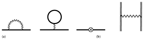
Figure 1.
Feynman diagrams of the first-order contributions to the energy shift of a single hole state. Wavy lines correspond to the photon propagators. The cross inside a circle represents a counterpotential term, −U. (a) The first-order one-electron Feynman diagrams in the redefined vacuum formalism, that correspond (from left to right) to SE, VP, and CP corrections. Single solid lines display the electron propagators in the redefined vacuum framework. (b) Two-electron one-photon-exchange and counterpotential Feynman diagrams. Double lines indicate the standard electron propagators in the external potential.
In the standard vacuum formulation, the latter contributions correspond to the one-photon-exchange and counterpotential diagrams, that are displayed in Figure 1b. The aim of the present subsection is to derive expressions for the interelectronic-interaction diagrams from the redefined vacuum formulation and demonstrate its equivalence to the standard one.
The starting point is the first-order term of the perturbative expansion of . Then the identification of different contributions in Equation (43) is performed to retrieve the one-photon-exchange correction. The Feynman rules provided in [42] lead to following Green’s function matrix element
for the SE graph, and
for the VP graph. The matrix element shorthand notation is defined as
it satisfies the transposition symmetry property
The interelectronic-interaction operator and its first derivative are defined as
where and is the photon propagator. Associated -symmetry properties hold both in the Feynman and Coulomb gauges,
According to Equation (34), which allows us to calculate the first-order correction to the energy shift, expressions (44) and (45) have second-order poles at . Hence the contour integrals enclose the first-order poles at , and the Green functions are evaluated to
At the moment, the first-order SE and VP energy corrections are evaluated within the redefined vacuum framework. Notice that these formulas describe both the one-photon exchange and the one-electron one-loop corrections. In order to extract the sought contribution of the one-photon exchange, the SE and VP corrections in the standard vacuum framework, and , respectively, are to be subtracted. Application of Equation (10) gives for the SE part,
and for the VP part,
with and .
The counterpotential graph remains to be evaluated. The corresponding Green function, with the definition , is found to be
Similar to the previous derivations, the contour integral evaluation yields
since CP does not contribute to the radiative corrections . Finally, the first-order interelectronic-interaction correction is given by
where the first two terms correspond to the one-photon exchange and the third one is the counterpotential term, cf. Figure 1b. Here one should notice, that this contribution differs by the minus sign from the valence-electron case [43]. It comes from the overall minus sign for the hole states case, see Equation (33). Moreover, since these three terms originate from individually gauge-invariant graphs, they are also separately gauge invariant.
4.2. Second-Order Contributions
The second-order contributions to the energy shift of the one-hole state in the redefined vacuum formalism are given only by the one-electron diagrams, depicted in Figure 2. Similar to the first order, these diagrams in addition to one-electron two-loop radiative corrections include also the two-electron (screened) one-loop radiative corrections and the contributions due to interaction between the hole and the closed-shell electrons. Therefore, we can formally represent the second-order energy correction (35) as follows,
where three different terms are present: the one-electron two-loop , the screened radiative , and the two-photon exchange terms. Similar to the first-order derivation, we extract the second and third contributions from the general formulas. First, applying the Feynman rules for each of the diagrams depicted in Figure 2 we write down the expression for the second-order Green function . The complete set is composed of ten two-loop diagrams [SESE, SEVP, VPVP, V(VP)P, V(SE)P, S(VP)E], which are presented on the left side of Figure 2. In the extended Furry picture, seven additional counterpotential diagrams [SECP, VPCP, CPCP] depicted on the right side of Figure 2 have to be considered as well. The next step is the identification of the one-electron two-loop radiative corrections. Details concerning this procedure are rather similar to the one-valence-electron case, which we considered in Reference [43]. For this reason, we do not provide here the full-length derivation and restrict ourselves to the presentation of final formulas.
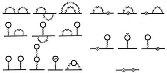
Figure 2.
One-electron two-loop (left group) and counterpotential (right group) Feynman diagrams representing the second-order contributions to the energy shift of a single-hole state in the redefined vacuum formalism. Notations for the diagrams are as follows, left group: SESE (first row); SEVP (second row); VPVP, V(VP)P, V(SE)P, and S(VP)E from left to right in the last row; right group: SECP (first row); VPCP (second row); CPCP (third row). Other notations are same as in Figure 1a.
4.2.1. Screened Radiative Corrections
Identifying the screened radiative corrections from the general expression for each diagram we arrive at,
where corresponding terms are explicitly given in Appendix A by Equations (A1)–(A6) and by Equations (A7) and (A8) for the counterpotential contributions. Such a decomposition allows us to identify eight gauge-invariant subsets based on the gauge invariance of the one-electron two-loop diagrams. Here are the subsets with labeling presented in Figure 2 and in Equation (58): VPVP, V(VP)P, SEVP, V(SE)P, S(VP)E, SESE, VPCP, and SECP. The identified subsets should be gauge invariant in both redefined and standard vacuum frameworks. It means that the screened radiative contributions obtained as a difference between the redefined and the standard vacuum expressions also form the same gauge-invariant subsets. Explicit proof of this statement has been performed for the two-photon-exchange subsets in the case of one-valence-electron in Reference [43].
In what follows, we also rearrange the screened radiative corrections according to its usual representation by the many-electron diagrams in the ordinary vacuum formalism, displayed in Figure 3:
where and represent the screened self-energy correction (vertex and wave-function parts), and correspond to the screened vacuum polarization contribution (wave-function and internal-loop parts), and, finally, is the counterpotential term. The self-energy vertex part is given by the expression,
which arises from the fourth sum in Equation (A3), the second one in Equation (A4), and the third one in Equation (A6). The self-energy wave-function part reads
where the third sum and second term of the fifth sum in Equation (A3), the first and third sums in Equation (A4), as well as the first, second, fourth, and fifth sums in Equation (A6) are added together. To keep track of the source of the generated reducible contributions, a subscript is used with previous notation; for example , where . The vacuum-polarization wave-function part reads,
which comes from Equation (A1), the first sum in Equation (A2), and the first and second sums as well as the first term in fifth sum and the sixth sum in Equation (A3). For the vacuum-polarization internal-loop term we obtain,
by adding the second sum in Equations (A2) and (A5). Finally, the counterpotential term reads,
found as the sums of Equations (A7) and (A8). The expressions above provide all contributions to the screened self-energy and vacuum polarization. Here, we note that the screened self-energy formulas perfectly agree with the ones of Reference [45], where they were obtained by considering the diagrams depicted in Figure 3 directly.
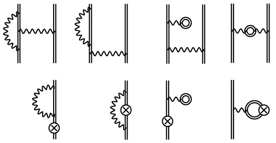
Figure 3.
Feynman diagrams representing the screened self-energy and vacuum-polarization corrections to the energy shift. Notations for the diagrams are as follows, SE,ver, SE,wf, VP,wf, and VP,int (upper raw) and CP (lower raw). Other notations are the same as in Figure 1b.
4.2.2. Two-Photon-Exchange Correction
Now let us proceed with the two-photon-exchange part. Here, we skip the details of the derivation, since it is rather similar to one presented in Reference [43], and come straight to the final expression for the total two-photon-exchange correction ,
which is given by a sum of Equations (A9)–(A26), presented in Appendix B. Each term in Equation (65) is individually gauge invariant. Generally, this statement is based on the gauge invariance of the corresponding subsets of one-electron diagrams depicted in Figure 2. More rigorously it has been proved in our recent paper [43] for the one-valence-electron case.
Similar to the previous consideration of the screened radiative corrections, one can present the two-photon-exchange contribution according to the many-electron diagrams, which are displayed in Figure 4.
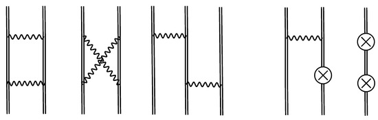
Figure 4.
Feynman diagrams representing the two-photon-exchange corrections to the energy shift. Notations for the diagrams are as follows, from left to right: two-electron ladder, two-electron cross, three-electron, and two counterpotential graphs. Other notations are the same as in Figure 1b.
Consequently, the two-photon-exchange term can be written as follows,
The two-electron ladder contribution is conveniently split into irreducible and reducible parts:
and
where the irreducible part comes from the second sum in Equations (A9) and (A15), while the reducible part is originating from the first sum in Equations (A10) and (A16). The irreducible and reducible parts of the two-electron cross contribution read,
and
which comes from the first sum in Equations (A9) and (A15) (irreducible), and from the second and third sums in (A10) (reducible). The prime on the sum in Equation (69) indicates the omission of particular terms, namely, for the first term in the curly brackets and for the second one. For the three-electron irreducible contributions, one ends up with the expression,
by summing up Equations (A11), (A13), (A17), (A19), (A21), and (A22). The three-electron reducible contribution is found by adding Equations (A12), (A14), (A18), and (A20) into,
The expressions above are derived for the first time and require a critical view. Therefore, in Appendix C, we apply the Breit approximation to our results and compare the outcome with the RMBPT expressions of Reference [40]. A complete agreement is found. Moreover, in Reference [40] it was demonstrated within the RMBPT framework that the expressions for a single-hole state turn into corresponding formulas for the valence electron with the replacement of h to v and multiplying on an overall minus sign. Here, we manifest that such a symmetry also holds within the QED framework.
5. Discussion and Conclusions
In recent years, the accuracy of large-scale correlation calculations of transition energies in many-electron atoms and ions drastically improved [2,44,53,54,55,56]. Various highly efficient computer codes have been developed for this purpose [57,58,59,60,61,62]. In view of this rapid progress, it becomes increasingly important to include the QED effects in these calculations as well. At present, such an account is mainly based on the approximate treatment via QED model potentials [63,64]. Even though effective methods provide access to higher-order contributions, it is usually not clear how one can estimate the accuracy of the results. In contrast, ab initio calculations are more accurate up to the corresponding order and allow a good control over uncertainties. However, ab initio QED calculations for many-electron atoms are a rather difficult problem. The first step towards these challenging calculations is to develop the framework that simplifies the derivation of the bound-state QED formulas. In the present paper, we have presented an efficient method, based on the vacuum redefinition and the two-time Green’s function approach, to derive calculation expressions within the rigorous QED framework. A redefined vacuum state allows one to drastically reduce the complexity of the many-electron ab initio QED formulation keeping only valence electrons or vacancies under consideration. Contributions to the binding energy are expressed in terms of Green’s function matrix elements with active particles (electrons or holes) only. The interaction of these active particles with the core electrons is included via the consideration of the radiative corrections, self-energy, and vacuum polarization. It has been explicitly demonstrated for the case of one active particle. We have shown that the method based on vacuum redefinition in QED is a well-suited tool to tackle atoms with a complicated electronic structure.
As an example, the method is applied to atoms with a single-hole electronic configuration, which occurs in halogen atoms such as fluorine, chlorine, etc. The particular interest in this system is twofold. First, in References [44,45,46] it was demonstrated that highly accurate theoretical predictions are possible in such atoms, and thus accurate tests of the QED effects become feasible. The reason for this is a drastic reduction of the correlations due to Layzer quenching effects [65]. Second, recent measurements of the fine-structure splitting in fluorine-like systems [47,48] emphasize the necessity of improvement in theoretical predictions for such systems. The accuracy of experimental results is at least of the same order as that of the theoretical predictions, while for some ions it is an order of magnitude better. Furthermore, an improvement in the experimental precision is foreseen in the near future [47]. Here, we have derived the formulas for the QED contributions up to the second order in for the single-hole configuration. The screened radiative and two-photon-exchange corrections have been carefully extracted from the rigorous formulas obtained within the redefined vacuum formalism. An important advantage of the employed formalism consists in the identification of gauge-invariant subsets, which is based on the corresponding subsets of one-electron diagrams. This feature can be very useful in future derivations of the higher-order contributions since it provides a robust verification. Finally, we have checked the results by the comparison of the Breit approximation applied to the derived expression with the previously obtained RMBPT expressions.
Author Contributions
Methodology, R.N.S., A.V.V., and D.A.G.; formal analysis, R.N.S.; investigation, R.N.S.; writing—original draft preparation, R.N.S.; writing—review and editing, R.N.S., A.V.V., D.A.G., and S.F.; supervision, A.V.V. and S.F. All authors have read and agreed to the published version of the manuscript.
Funding
This work was supported by DFG (VO1707/1-3) and by RFBR (Grant No. 19-02-00974). A.V.V. acknowledges financial support by the Government of the Russian Federation through the ITMO Fellowship and Professorship Program. D.A.G. acknowledges the support by the Foundation for the Advancement of Theoretical Physics and Mathematics “BASIS”.
Institutional Review Board Statement
Not applicable.
Informed Consent Statement
Not applicable.
Data Availability Statement
Not applicable.
Conflicts of Interest
The authors declare no conflict of interest.
Appendix A. Gauge-Invariant Subsets of the Screened Radiative Diagrams
The eight different gauge invariant subsets for the screened radiative corrections previously introduced in the main text, see Equation (58), are presented here. Let us start with the two terms, which originate from the one-electron diagrams with VP loop only: VPVP and V(VP)P,
and
respectively. The next three subsets displayed come from the diagrams with both SE and VP loops. We begin with the SEVP term, where the disconnected SEVP contribution (second term in Equation (35)) is included,
The second subset that falls into this category is the V(SE)P one,
and finally the S(VP)E term yields
Finally, the SESE subset comes from the diagrams with only self-energy loops. It includes also the SESE disconnected contribution (second term in Equation (35)), and leads to the following expression,
Furthermore, in the extended Furry picture, two counterpotential subsets emerge. The first one, VPCP, is associated with a vacuum-polarization loop,
while the second, SECP, arises from the diagram with a self-energy loop and the disconnected SECP part (second term in Equation (35)),
Appendix B. Gauge-Invariant Subsets of the Two-Photon-Exchange Diagrams
The eleven different gauge invariant subsets of the two-photon-exchange contributions previously introduced in the main text (see Equation (65)) are presented here. Let us start with the two subsets originating from the diagrams with self-energy loops only. We present the two- and three-electron contributions separately. The two-electron irreducible and reducible SESE terms are
and
where the prime on the sum means that the terms are excluded from the summation. The three-electron SESE subset consists of the irreducible part,
and the reducible part,
Now we focus on the four subsets with mixed SE and VP loops. The SEVP subset has only three-electron contribution, the irreducible part of which is given by
The corresponding reducible part merged with the disconnected SEVP contribution yields,
The next two subsets are S(VP)E and V(SE)P. The two-electron S(VP)E contributions are
and
where the prime on the sum means that the term is excluded from the summation. The irreducible contribution of the three-electron S(VP)E subset yields
and the reducible one reads
The last subset in this category is V(SE)P, which comprises only the three-electron contributions: irreducible,
and reducible,
Finally, the two subsets originating from the diagrams with vacuum-polarization loops only are the VPVP subset,
and the V(VP)P subset,
Both of them have only three-electron parts.
Within the extended Furry picture, three extra counterpotential subsets emerge. The first one, SECP, is related to the self-energy loop, the irreducible contribution of which is
The corresponding reducible part encapsulating the disconnected SECP contribution can be written as
The second one, VPCP, is expressed by
Finally, the last subset, CPCP, reads
Appendix C. Two-Photon Exchange: Comparison between QED and RMBPT
To achieve the sought matching between QED and RMBPT, we apply the Breit approximation to the expressions presented in Section 4.2.2. To this end, let us first introduce the interelectronic-interaction operator in the Breit approximation:
where “C” means the Coulomb gauge. Since is -independent, the reducible contributions, which contain derivatives of I, vanish within this approximation. The second implication of the Breit approximation is to consider only the positive-energy states in summations, i.e.,
where now i (and later j) means only positive-energy state, m (and later n) is an excited state, , and a (and b) denotes one of the core states, . We first apply the Breit approximation to the three-electron contributions given by Equations (71) and (72) and to the counterpotential term, Equation (73), which are transformed as follows,
and
The summations were rewritten using Equation (A28). Notice that the core electrons contributions vanish altogether upon relabeling the indices and applying the symmetry properties (47). Furthermore, sums involving in the denominators are kept intact since the hole energy lies in the positive-energy spectrum, and the replacement also allows one to remove the restrictions in all the other sums.
It is left to evaluate the two-electron contributions. Recall that the integration path closes in the upper half of the complex plane to consider only positive intermediate energy states and that no reducible contributions are present. Let us divide the expressions in Equations (67) and (69) into direct and exchange parts, namely, the first term in each is the direct contribution and the second is the exchange one. We start by showing that both cross contributions vanish due to their pole structure. The cross-exchange poles are and the cross-direct poles are and , for . It leads to the corresponding residue integration
Next, we inspect the ladder poles, which are found to be in and , same for both direct and exchange parts. Performing the Cauchy integration, one finds
where the first term in the last line is the one we are looking for, while the second one compensates the fourth sum in Equation (A29). Thus, the final expression for the two-photon exchange within the Breit approximation yields
which is in full agreement with the RMBPT result of Reference [40].
References
- Furry, W.H. On Bound States and Scattering in Positron Theory. Phys. Rev. 1951, 81, 115. [Google Scholar] [CrossRef]
- Kozlov, M.G.; Safronova, M.S.; Crespo López-Urrutia, J.R.; Schmidt, P.O. Highly charged ions: Optical clocks and applications in fundamental physics. Rev. Mod. Phys. 2018, 90, 045005. [Google Scholar] [CrossRef]
- Karshenboim, S.G. Precision physics of simple atoms: QED tests, nuclear structure and fundamental constants. Phys. Rep. 2005, 422, 1–63. [Google Scholar] [CrossRef]
- Yerokhin, V.A.; Shabaev, V.M. Lamb Shift of n = 1 and n = 2 States of Hydrogen-like Atoms, 1 ≤ Z ≤ 110. J. Phys. Chem. Ref. Data 2015, 44, 033103. [Google Scholar] [CrossRef]
- Mohr, P.J.; Newell, D.B.; Taylor, B.N. CODATA Recommended Values of the Fundamental Physical Constants: 2014. J. Phys. Chem. Ref. Data 2016, 45, 043102. [Google Scholar] [CrossRef]
- Pohl, R.; Antognini, A.; Nez, F.; Amaro, F.D.; Biraben, F.; Cardoso, J.M.R.; Covita, D.S.; Dax, A.; Dhawan, S.; Fernandes, L.M.P.; et al. The size of the proton. Nature 2010, 466, 213. [Google Scholar] [CrossRef] [PubMed]
- Antognini, A.; Nez, F.; Schuhmann, K.; Amaro, F.D.; Biraben, F.; Cardoso, J.M.R.; Covita, D.S.; Dax, A.; Dhawan, S.; Diepold, M.; et al. Proton Structure from the Measurement of 2S-2P Transition Frequencies of Muonic Hydrogen. Science 2013, 339, 417–420. [Google Scholar] [CrossRef]
- Karr, J.P.; Marchand, D.; Voutier, E. The proton size. Nat. Rev. Phys. 2020, 2, 601. [Google Scholar] [CrossRef]
- Puchalski, M.; Szalewicz, K.; Lesiuk, M.; Jeziorski, B. QED calculation of the dipole polarizability of helium atom. Phys. Rev. A 2020, 101, 022505. [Google Scholar] [CrossRef]
- Yerokhin, V.A.; Patkóš, V.; Puchalski, M.; Pachucki, K. QED calculation of ionization energies of 1snd states in helium. Phys. Rev. A 2020, 102, 012807. [Google Scholar] [CrossRef]
- Patkóš, V.; Yerokhin, V.A.; Pachucki, K. Complete α7m Lamb shift of helium triplet states. Phys. Rev. A 2021, 103, 042809. [Google Scholar] [CrossRef]
- Zheng, X.; Sun, Y.; Chen, J.J.; Jiang, W.; Pachucki, K.; Hu, S.M. Measurement of the Frequency of the 23S − 23P Transition of 4He. Phys. Rev. Lett. 2017, 119, 263002. [Google Scholar] [CrossRef]
- Thomas, K.F.; Ross, J.A.; Henson, B.M.; Shin, D.K.; Baldwin, K.G.H.; Hodgman, S.S.; Truscott, A.G. Direct Measurement of the Forbidden 23S1 → 33S1 Atomic Transition in Helium. Phys. Rev. Lett. 2020, 125, 013002. [Google Scholar] [CrossRef]
- Pachucki, K.; Sapirstein, J. Determination of the fine structure constant from helium spectroscopy. J. Phys. B 2002, 35, 1783–1793. [Google Scholar] [CrossRef]
- Pachucki, K.; Patkóš, V.; Yerokhin, V.A. Testing fundamental interactions on the helium atom. Phys. Rev. A 2017, 95, 062510. [Google Scholar] [CrossRef]
- Gumberidze, A.; Stöhlker, T.; Banaś, D.; Beckert, K.; Beller, P.; Beyer, H.F.; Bosch, F.; Hagmann, S.; Kozhuharov, C.; Liesen, D.; et al. Quantum electrodynamics in strong electric fields: The ground-state Lamb shift in hydrogenlike uranium. Phys. Rev. Lett. 2005, 94, 223001. [Google Scholar] [CrossRef]
- Indelicato, P. QED tests with highly charged ions. J. Phys. B 2019, 52, 232001. [Google Scholar] [CrossRef]
- Yerokhin, V.A.; Indelicato, P.; Shabaev, V.M. Two-loop self-energy correction in high-Z hydrogenlike ions. Phys. Rev. Lett. 2003, 91, 073001. [Google Scholar] [CrossRef] [PubMed]
- Gassner, T.; Trassinelli, M.; Heß, R.; Spillmann, U.; Banaś, D.; Blumenhagen, K.H.; Bosch, F.; Brandau, C.; Chen, W.; Dimopoulou, C.; et al. Wavelength-dispersive spectroscopy in the hard x-ray regime of a heavy highly-charged ion: The 1s Lamb shift in hydrogen-like gold. New J. Phys. 2018, 20, 073033. [Google Scholar] [CrossRef]
- Gumberidze, A.; on behalf of the SPARC Collaboration. Atomic physics at the future facility for antiproton and ion research: A status report. Phys. Scr. 2013, T156, 014084. [Google Scholar] [CrossRef]
- Blundell, S.A.; Mohr, P.J.; Johnson, W.R.; Sapirstein, J. Evaluation of two-photon exchange graphs for highly charged heliumlike ions. Phys. Rev. A 1993, 48, 2615. [Google Scholar] [CrossRef]
- Persson, H.; Salomonson, S.; Sunnergren, P.; Lindgren, I. Two-electron Lamb-shift calculations on heliumlike ions. Phys. Rev. Lett. 1996, 76, 204. [Google Scholar] [CrossRef] [PubMed]
- Mohr, P.J.; Sapirstein, J. Evaluation of two-photon exchange graphs for excited states of highly charged heliumlike ions. Phys. Rev. A 2000, 62, 052501. [Google Scholar] [CrossRef]
- Artemyev, A.N.; Shabaev, V.M.; Yerokhin, V.A.; Plunien, G.; Soff, G. QED calculation of the n = 1 and n = 2 energy levels in He-like ions. Phys. Rev. A 2005, 71, 062104. [Google Scholar] [CrossRef]
- Malyshev, A.V.; Kozhedub, Y.S.; Glazov, D.A.; Tupitsyn, I.I.; Shabaev, V.M. QED calculations of the n = 2 to n = 1 x-ray transition energies in middle-Z heliumlike ions. Phys. Rev. A 2019, 99, 010501. [Google Scholar] [CrossRef]
- Kozhedub, Y.S.; Malyshev, A.V.; Glazov, D.A.; Shabaev, V.M.; Tupitsyn, I.I. QED calculation of electron-electron correlation effects in heliumlike ions. Phys. Rev. A 2019, 100, 062506. [Google Scholar] [CrossRef]
- Sapirstein, J.; Cheng, K.T. Determination of the two-loop Lamb shift in lithiumlike bismuth. Phys. Rev. A 2001, 64, 022502. [Google Scholar] [CrossRef]
- Yerokhin, V.A.; Artemyev, A.N.; Shabaev, V.M.; Sysak, M.M.; Zherebtsov, O.M.; Soff, G. Evaluation of the two-photon exchange graphs for the 2p1/2 − 2s transition in Li-like ions. Phys. Rev. A 2001, 64, 032109. [Google Scholar] [CrossRef]
- Artemyev, A.N.; Shabaev, V.M.; Sysak, M.M.; Yerokhin, V.A.; Beier, T.; Plunien, G.; Soff, G. Evaluation of the two-photon exchange diagrams for the (1s)22p3/2 electron configuration in Li-like ions. Phys. Rev. A 2003, 67, 062506. [Google Scholar] [CrossRef]
- Sapirstein, J.; Cheng, K.T. S-matrix calculations of energy levels of the lithium isoelectronic sequence. Phys. Rev. A 2011, 83, 012504. [Google Scholar] [CrossRef]
- Malyshev, A.V.; Volotka, A.V.; Glazov, D.A.; Tupitsyn, I.I.; Shabaev, V.M.; Plunien, G. QED calculation of the ground-state energy of berylliumlike ions. Phys. Rev. A 2014, 90, 062517. [Google Scholar] [CrossRef]
- Malyshev, A.V.; Volotka, A.V.; Glazov, D.A.; Tupitsyn, I.I.; Shabaev, V.M.; Plunien, G. Ionization energies along beryllium isoelectronic sequence. Phys. Rev. A 2015, 92, 012514. [Google Scholar] [CrossRef]
- Malyshev, A.V.; Glazov, D.A.; Kozhedub, Y.S.; Anisimova, I.S.; Kaygorodov, M.Y.; Shabaev, V.M.; Tupitsyn, I.I. Ab initio Calculations of Energy Levels in Be-Like Xenon: Strong Interference between Electron-Correlation and QED Effects. Phys. Rev. Lett. 2021, 126, 183001. [Google Scholar] [CrossRef]
- Artemyev, A.N.; Shabaev, V.M.; Tupitsyn, I.I.; Plunien, G.; Yerokhin, V.A. QED calculation of the 2p3/2 − 2p1/2 transition energy in boronlike argon. Phys. Rev. Lett. 2007, 98, 173004. [Google Scholar] [CrossRef]
- Artemyev, A.N.; Shabaev, V.M.; Tupitsyn, I.I.; Plunien, G.; Surzhykov, A.; Fritzsche, S. Ab initio calculations of the 2p3/2 − 2p1/2 fine-structure splitting in boronlike ions. Phys. Rev. A 2013, 88, 032518. [Google Scholar] [CrossRef]
- Malyshev, A.V.; Glazov, D.A.; Volotka, A.V.; Tupitsyn, I.I.; Shabaev, V.M.; Plunien, G.; Stöhlker, T. Ground-state ionization energies of boronlike ions. Phys. Rev. A 2017, 96, 022512. [Google Scholar] [CrossRef]
- Sapirstein, J.; Cheng, K.T. S-matrix calculations of energy levels of sodiumlike ions. Phys. Rev. A 2015, 91, 062508. [Google Scholar] [CrossRef]
- Lindgren, I.; Morrison, J. Atomic Many-Body Theory; Springer: Berlin, Germany, 1985. [Google Scholar]
- Avgoustoglou, E.; Johnson, W.; Plante, D.; Sapirstein, J.; Sheinerman, S.; Blundell, S. Many-body perturbation-theory formulas for energy levels of excited states of closed-shell atoms. Phys. Rev. A 1992, 46, 5478. [Google Scholar] [CrossRef]
- Johnson, W.R.; Sapirstein, J.; Cheng, K.T. Theory of 2s1/2-2p3/2 transitions in highly ionized uranium. Phys. Rev. A 1995, 51, 297–302. [Google Scholar] [CrossRef]
- Johnson, W.R. Atomic Structure Theory. Lectures on Atomic Physics; Springer: Berlin/Heidelberg, Germany, 2007. [Google Scholar]
- Shabaev, V.M. Two-time Green’s function method in quantum electrodynamics of high-Z few-electron atoms. Phys. Rep. 2002, 356, 119. [Google Scholar] [CrossRef]
- Soguel, R.N.; Volotka, A.V.; Tryapitsyna, E.V.; Glazov, D.A.; Kosheleva, V.P.; Fritzsche, S. Redefined vacuum approach and gauge-invariant subsets in two-photon-exchange diagrams for a closed-shell system with a valence electron. Phys. Rev. A 2021, 103, 042818. [Google Scholar] [CrossRef]
- Li, M.C.; Si, R.; Brage, T.; Hutton, R.; Zou, Y.M. Proposal of highly accurate tests of Breit and QED effects in the ground state 2p5 of the F-like isoelectronic sequence. Phys. Rev. A 2018, 98, 020502. [Google Scholar] [CrossRef]
- Volotka, A.V.; Bilal, M.; Beerwerth, R.; Ma, X.; Stöhlker, T.; Fritzsche, S. QED radiative corrections to the 2P1/2 − 2P3/2 fine structure in fluorinelike ions. Phys. Rev. A 2019, 100, 010502. [Google Scholar] [CrossRef]
- Shabaev, V.; Tupitsyn, I.; Kaygorodov, M.; Kozhedub, Y.; Malyshev, A.; Mironova, D. QED corrections to the 2P1/2 − 2P3/2 fine structure in fluorinelike ions: Model Lamb-shift-operator approach. Phys. Rev. A 2020, 101, 052502. [Google Scholar] [CrossRef]
- O’Neil, G.; Sanders, S.; Szypryt, P.; Gall, A.; Yang, Y.; Brewer, S.M.; Doriese, R.; Fowler, J.; Naing, A.; Swetz, D.; et al. Measurement of the 2P1/2 − 2P3/2 fine-structure splitting in fluorinelike Kr, W, Re, Os, and Ir. Phys. Rev. A 2020, 102, 032803. [Google Scholar] [CrossRef]
- Lu, Q.; Yan, C.L.; Xu, G.Q.; Fu, N.; Yang, Y.; Zou, Y.; Volotka, A.V.; Xiao, J.; Nakamura, N.; Hutton, R. Direct measurements for the fine-structure splitting of S viii and Cl ix. Phys. Rev. A 2020, 102, 042817. [Google Scholar] [CrossRef]
- Shabaev, V.M. Quantum electrodynamic theory of multiply charged ions. Sov. Phys. J. 1990, 33, 660–670. [Google Scholar] [CrossRef]
- Mohr, P.J.; Plunien, G.; Soff, G. QED corrections in heavy atoms. Phys. Rep. 1998, 293, 227. [Google Scholar] [CrossRef]
- Lindgren, I.; Salomonson, S.; Åsén, B. The covariant-evolution-operator method in bound-state QED. Phys. Rep. 2004, 389, 161. [Google Scholar] [CrossRef]
- Yu, O.A.; Labzowsky, L.N.; Plunien, G.; Solovyev, D.A. QED theory of the spectral line profile and its applications to atoms and ions. Phys. Rep. 2008, 455, 135. [Google Scholar]
- Dzuba, V.A.; Flambaum, V.V.; Schiller, S. Testing physics beyond the standard model through additional clock transitions in neutral ytterbium. Phys. Rev. A 2018, 98, 022501. [Google Scholar] [CrossRef]
- Si, R.; Guo, X.L.; Brage, T.; Chen, C.Y.; Hutton, R.; Froese Fischer, C. Breit and QED effects on the 3d92D3/2 → 2D5/2 transition energy in Co-like ions. Phys. Rev. A 2018, 98, 012504. [Google Scholar] [CrossRef]
- Imanbaeva, R.T.; Kozlov, M.G. Configuration Interaction and Many-Body Perturbation Theory: Application to Scandium, Titanium, and Iodine. Ann. Phys. 2019, 531, 1800253. [Google Scholar] [CrossRef]
- Cheung, C.; Safronova, M.S.; Porsev, S.G.; Kozlov, M.G.; Tupitsyn, I.I.; Bondarev, A.I. Accurate Prediction of Clock Transitions in a Highly Charged Ion with Complex Electronic Structure. Phys. Rev. Lett. 2020, 124, 163001. [Google Scholar] [CrossRef]
- Jönsson, P.; Gaigalas, G.; Bieroń, J.; Froese Fischer, C.; Grant, I.P. New version: Grasp2K relativistic atomic structure package. Comput. Phys. Commun. 2013, 184, 2197. [Google Scholar] [CrossRef]
- Kozlov, M.; Porsev, S.; Safronova, M.; Tupitsyn, I. CI-MBPT: A package of programs for relativistic atomic calculations based on a method combining configuration interaction and many-body perturbation theory. Comput. Phys. Commun. 2015, 195, 199–213. [Google Scholar] [CrossRef]
- Fritzsche, S. A fresh computational approach to atomic structures, processes and cascades. Comput. Phys. Commun. 2019, 240, 1. [Google Scholar] [CrossRef]
- Cheung, C.; Safronova, M.; Porsev, S. Scalable Codes for Precision Calculations of Properties of Complex Atomic Systems. Symmetry 2021, 13, 621. [Google Scholar] [CrossRef]
- Dzuba, V. Calculation of Polarizabilities for Atoms with Open Shells. Symmetry 2020, 12, 1950. [Google Scholar] [CrossRef]
- Fritzsche, S.; Palmeri, P.; Schippers, S. Atomic Cascade Computations. Symmetry 2021, 13, 520. [Google Scholar] [CrossRef]
- Ginges, J.S.M.; Berengut, J.C. Atomic many-body effects and Lamb shifts in alkali metals. Phys. Rev. A 2016, 93, 052509. [Google Scholar] [CrossRef]
- Tupitsyn, I.I.; Kozlov, M.G.; Safronova, M.S.; Shabaev, V.M.; Dzuba, V.A. Quantum Electrodynamical Shifts in Multivalent Heavy Ions. Phys. Rev. Lett. 2016, 117, 253001. [Google Scholar] [CrossRef]
- Layzer, D.; Bahcall, J. Relativistic Z-Dependent Theory of Many-Electron Atoms. Ann. Phys. 1962, 17, 177. [Google Scholar] [CrossRef]
Publisher’s Note: MDPI stays neutral with regard to jurisdictional claims in published maps and institutional affiliations. |
© 2021 by the authors. Licensee MDPI, Basel, Switzerland. This article is an open access article distributed under the terms and conditions of the Creative Commons Attribution (CC BY) license (https://creativecommons.org/licenses/by/4.0/).