Abstract
A fundamental phenomenon of coherent control is investigated theoretically using the example of neon photoionization by the bichromatic field of a free-electron laser. A system exposed to coherent fields with commensurable frequencies loses some symmetry, which manifests itself in the angular distribution and spin polarization of the electron emission. We predict several such effects, for example, the violation of symmetry with respect to the plane perpendicular to the polarization vector of the second harmonic and the appearance of new components of spin polarization. Furthermore, we predict a very efficient control of spin polarization via manipulation of the phase between the harmonics. Experimental observation of these effects is accessible with modern free-electron lasers operating in the extreme ultraviolet wavelength regime.
1. Introduction
Spin is a fundamental property of particles and plays a crucial role at any level of matter from elementary particles to macroscopic objects, such as magnets and even white dwarfs. It is of a great practical importance for spintronics, ionic traps, laser cooling, quantum computers, and other fields [1,2,3,4,5]. Production and detection of spin-polarized electrons emitted in photoionization of a gas target is more challenging in comparison with the ionization of condensed matter because the former targets are dilute and tend to be randomly oriented. There are two necessary prerequisites for nonzero photoelectron spin polarization: (i) the symmetry of the process contains a screw (axial vector(s)) and (ii) noticeable spin–orbit interaction. The latter allows for distinguishing spin states of the target atom or the residual ion, or of the electron in continuum. The directions of the axial vectors correspond to possible photoelectron spin components.
Some well known examples are as follows: (a) The Fano effect of the electron spin polarization in atomic photoionization by circularly polarized light [6,7,8]. The electrons are collected over the full solid angle 4. The screw is provided by the light helicity, while the spin–orbit interaction of the photoelectron provides selectivity of the spin states in the Cooper minimum of the cross section. Only one electron spin component parallel to the light beam is possible. The linearly polarized light does not produce the integral spin polarization because it is lacking the screw. (b) Spin polarization in angle-resolved electron emission from unpolarized atoms, produced by linearly polarized light (so-called ‘dynamic’ polarization) [9]. Within the electric dipole approximation, the screw is given by the vector product of the electric field and the direction of the electron emission. The selectivity of spin states is provided either by resolving initial atomic or final ionic fine-structure [10], or by spin–orbit interaction of the photoelectron [11]. Only the spin component normal to the reaction plane is possible. (c) Same as (b) but with circularly polarized light (so-called ‘polarization transfer’). Here, an additional screw appears due to the light helicity and all three components of the photoelectron spin generally occur.
Thus, the breaking of symmetry, which introduces additional distinguishable directions into the process, leads to new or to a change of already existing spin components of the photoelectron. One can also be reminded of further examples from molecular photoionization [9] and strong-field ionization [12,13,14,15].
An important example of the symmetry violation is atomic ionization by light containing a coherent sum of components with commensurable frequencies. Consider the photoelectron angular distribution (PAD) in bichromatic ionization by the first () and second () harmonics,
often called the + process. For colinearly polarized incoherent harmonics, in the dipole approximation, the PADs are axially symmetric and possess a plane of symmetry perpendicular to this symmetry axis. The symmetry axis is directed along the electric field vector or along the photon beams direction for linearly and circularly polarized photons, respectively. Similar symmetries occur for one circularly polarized and another for linearly polarized harmonics, when the direction of the former beam is along the electric field of the latter. In this case, the electric field vector points out of the reaction plane.
However, when the two harmonics are coherently added, i.e., their relative phase is fixed, the PADs lose part of the symmetry. Examples of such a violation are shown in Figure 1 for cases when the resulting electric field strength changes in one (Figure 1a) or two (Figure 1b,c) dimensions. Changing the relative phase and the strength of harmonics provides a way to control the PADs as it was realized in the + process 30 years ago in the optical domain [16,17,18]. Recently, with the advent of longitudinally coherent free-electron lasers, experimental studies of the coherent control in the + process in the XUV wavelength range became possible and the first such measurements have been done [19,20,21].
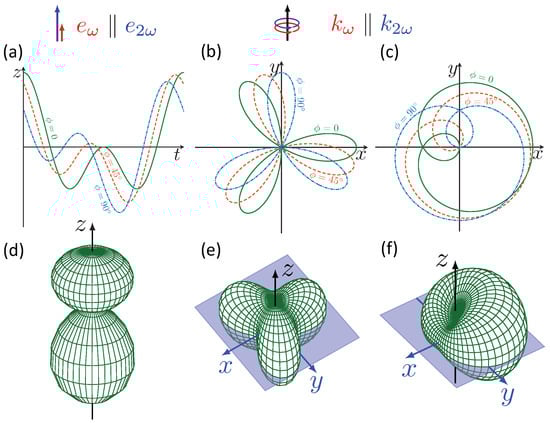
Figure 1.
Electric field strength of coherent bichromatic fields (a–c) and corresponding typical PADs (d–f): (a,d) time dependence of the linearly polarized bichromatic field and the corresponding PAD having symmetry; (b,e) trajectory of the amplitude of the bichromatic field with the circularly polarized counter rotating harmonics and the corresponding PAD having symmetry; (c,f) similar to (b,e) but for co-rotating components and corresponding PAD having symmetry ( for ionization of an s-shell [25]). The harmonic intensity ratio is chosen differently for different panels for better visualization.
As follows from the above consideration, the photoelectron spin polarization can gain new components and change the existing components in + ionization in comparison with the case of incoherent and beams. The spin polarization may be controlled by changing relative strength and phase of the two harmonics in the + ionization, taking advantage of the two ionization pathways: single photon ionization by the second harmonic and two-photon ionization by the first harmonic . Recently, we analyzed these effects in the + process for collinear circularly polarized beams and linearly polarized beams with parallel electric field vectors on the example of the neon atom in the region of the – excitations [22]. The selectivity with respect to the spin states was provided by the fine-structure splitting of these intermediate resonances in the two-photon ionization pathway.
Spin polarization control in the gas phase has not been realized yet. However, spin-polarized currents in semiconductors were controlled through quantum interference in one- and two-photon absorption of two orthogonal linearly polarized harmonics [23,24]. This was one of the reasons to extend our previous study of the photoelectron spin polarization in the + process [22] to the case of beams linearly polarized in the orthogonal directions.
The paper is organized as follows: Section 2 presents a short sketch of the theoretical approach. In contrast to our previous paper [22], we develop the formalism in the jK-coupling scheme of the angular momenta, which is more appropriate for the intermediate states in the noble gas atoms. The results are presented and discussed in Section 3. We first outline, for further comparison, some features of the electron spin polarization in one- and two-photon ionization and for bichromatic ionization by linearly polarized harmonics with parallel electric fields. Then, we turn to the case of crossed linearly polarized harmonics. The final section is devoted to our conclusions. Cumbersome formalism and details of the atomic model for calculating the dipole matrix elements are moved to Appendix A.
2. Theoretical Description
The combined electric field of the fundamental () and second harmonic () is taken in the form
where () is the pulse envelope, denotes the relative phase between the two harmonics, and and are their intensities. We set the z-axis along the (unit) polarization vector of the fundamental harmonic , while one of the second harmonic may be either parallel, , or orthogonal, (see Figure 2a).
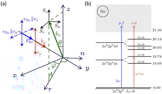
Figure 2.
(a) The coordinate systems: laboratory and for spin observation . The z-axis is chosen parallel to the electric field of the beam with fundamental frequency , the y-axis is along the direction of the beam propagation, the -axis belongs to the plane spanned by the electric vector of the beam with the second harmonic (z-axis), and the direction of the electron emission direction; the n-axis is normal to the latter plane; (b) scheme of the bichromatic + ionization in Ne at between 19.0 and 20.2 eV.
The spin density matrix of electrons with energy IP (IP is the ionization potential) in the lowest non-vanishing order perturbation theory is expressed as
where define the direction of the electron emission, is the amplitude of ionization by the second harmonic with a frequency of in the first order of perturbation theory, and is the amplitude of ionization by photons with frequency in the second order of perturbation theory; and are the magnetic quantum numbers of the initial atomic and final ionic states, respectively, and is the spin projection of the photoelectron. We have assumed a chaotically oriented angular momentum of the initial atomic state. Following the non-stationary perturbation theory [26], we write down
Here, is the operator of the atomic electric dipole momentum and and are field-dependent factors which are given by Equations (A8) and (A9) of Appendix A.
The density matrix (3) is parameterized in terms of the spin components [27]:
where , , and are the components of the spin polarization vector in an arbitrary (but fixed) coordinate system. We choose here the coordinate system ‘’ shown in Figure 2a with the linear momentum of the photoelectron lying in the plane . Combining (3)–(6), the spin components can be expressed in terms of the dipole matrix elements. We construct , and, hence, statistical tensors (3) in the jK-coupling scheme [27] in terms of bilinear combinations of the partial-wave components of ionization amplitudes (see Appendix A for details).
Usually, spin polarization of photoelectrons is studied for heavy atoms where the fine-structure can be energetically resolved in the photoelectron spectrum [8,15,28]. Similar to [22], we take a comparatively light neon atom in order to focus on coherent control of the photoelectron spin due to the fine-structure splitting of the intermediate resonances in the two-photon ionization pathway. We suppose that the fine structure of electrons in the continuum is unresolved.
For an illustrative example, we present data for neon ionization with the fundamental frequency in the region of the and resonances. The scheme of the + process is depicted in Figure 2b. Bound–bound and bound–continuum matrix elements are computed with the semi-relativistic version of the B-spline R-matrix code [29] in the length form, taking full account of non-orthogonality of the electron orbitals (see Appendix B for details).
3. Results and Discussion
The number of optical cycles in the numerical calculations, except when scanning the pulse duration, was set to . The latter corresponds in our case to the full pulse duration of ≈100 fs. The intensity of the fundamental harmonic was taken as W/cm, while the intensity of the second harmonic was chosen as 0.1% of the fundamental. At this intensity ratio, we found the strongest effect of interference between the two pathways in the energy region of interest.
3.1. Photoelectron Spin Polarization in Two-Photon Ionization
Spin polarization of photoelectrons in the two-photon ionization by linearly polarized light with constant intensity was considered in [28,30]. The parameterization of the spin polarization for pulses with finite time duration remains the same as in [30],
where is the spin component normal to the reaction plane (Figure 2a). Other electron spin components vanish. The axial symmetric normalized PAD (NPAD) can be cast into the form
where is the Legendre polynomial. Note that k takes only even values and therefore the PAD possesses symmetry with the plane of symmetry perpendicular to the electric field (Figure 3a). The NPAD (8) is calculated as a trace of the density matrix (3) over the spin projections, . The anisotropy parameters and the spin parameters are expressed in terms of bilinear combinations of the partial-wave components of and (see Appendix A, the comment after Equation (A23)).
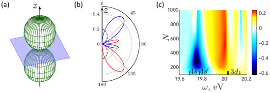
Figure 3.
(a) Typical NPAD for two-photon ionization; (b) for the photon energy corresponding to the resonance (19.78 eV). The dashed black line shows PAD (arbitrary units); solid red (blue) lines show positive (negative) values of the spin polarization. (c) 2D-map of , where is the ‘magic’ angle, in the region of and resonances as a function of the number of optical cycles N.
Figure 3b shows (7) for the carrier frequency , corresponding to the energy of the resonance. Calculated maximal values of are as high as .
The dependence of on the pulse duration at the ‘magic angle’ (at this angle, ) is shown by the 2D-map in Figure 3c. By increasing the time duration, the spectral width of the pulse decreases and the resonances in values of the spin polarization become sharper. Interestingly, by increasing the duration, increases in the resonances and attenuates in the resonances. It may be attributed to the fact that the dynamic spin polarization vanishes in the case of a single ionization channel [31]. The latter is a limiting case when all processes proceed via the single s intermediate state and, therefore, all photoelectrons are described by the p wave of the continuum. Then, the case of single-channel ionization is realized provided the spin–orbit interaction is neglected in the initial and final atomic states, as in our model. For the intermediate states, at least two ionization channels leading to p and f continua are present.
3.2. Parallel Polarization Vectors
We focus here on effects of symmetry violation; a more detailed discussion of this case can be found in [22]. For parallel polarizations, , the PAD keeps the axial symmetry but shows ‘forward/backward asymmetry’ (see Figure 4a) [22,25]. The NPAD is now given by the expression
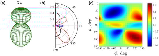
Figure 4.
(a) Typical NPAD for parallel electric fields of the coherent harmonics. (b) for in the vicinity of the resonance (19.78 eV). The black line corresponds to the PAD (arbitrary units are the same as in Figure 3a); solid red (blue) lines show positive (negative) values of the spin polarization. (c) at 19.78 eV, controlled by variation of the phase between the fields .
Note that terms with odd Legendre polynomials now contribute into the NPAD, causing the above asymmetry and reducing its symmetry from of (8) to of (9).
Since , new spin components, in addition to , do not appear. However, the forward-backward asymmetry strongly affects the degree of spin polarization
Expressions for the parameters , are given by Equations (A16)–(A23). Similar to the asymmetry of the NPAD (9) [22,25], the spin polarization (10) can be controlled by the variation of the relative phase between the fields and their relative strength. Such a control on (10) is demonstrated in Figure 4b,c in the region of the resonance. The modulation of at a fixed with varying relative phase of the harmonics reaches values of 0.6 at the angles around 50 and 130.
As a result of symmetry violation with respect to the -plane (), photoelectrons emitted in this plane may be polarized. This polarization is described by the term with in Equation (10).
3.3. Orthogonal Polarization Vectors
The axial symmetry is violated in this case. With and , and are the planes of symmetry (see Figure 5a) and the NPAD can be cast into the form
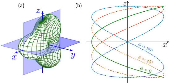
Figure 5.
(a) Typical NPAD for orthogonal electric fields of the coherent harmonics. Two planes of symmetry are shown: plane spanned by the electric fields and plane perpendicular to the polarization of the field with fundamental frequency ; (b) electric field of the two coherent harmonics at three different relative phases of the harmonics .
The last term with odd values of k represents a contribution of the interference between one- and two-photon ionization pathways. The parameters , are given by Equations (A24)–(A28). Parameters being the incoherent sum of those for one- and two-photon processes are interrelated with and : , see Equations (A15), (A16), (A24), (A25), and , see Equations (A17) and (A26). Figure 5b clarifies the reason of symmetry violation with respect to the plane. Due to the locked phases of the two harmonics, the end of the electric field vector depicts one of the Lissajous figures for the frequency ratio 1:2, which may be symmetric with respect to the plane only for . The field configuration keeps the forward-backward symmetry, which is similar to the circularly polarized radiation [25]. However, varying the relative phase between the fields with orthogonal polarizations changes the values of the anisotropy parameters, in contrast to the + ionization with circular polarized fields, when varying , causes space rotation of the PAD.
In comparison with the previous cases with axial symmetry, new spin components, and , appear as a result of the axial symmetry violation:
The parameters , , are given by Equations (A29)–(A35). Equivalently to Equations (13) and (14), one can write down the spin components and (see Equations (A36) and (A37)). The appearance of the spin components and is related to new screws, introduced by the vector products and , which decreases the symmetry of the system (atom + field) from the axial symmetry with axis z to the symmetry with axis x. The symmetry of PAD with respect to the -plane is a result of the bichromatic field with the frequency ratio 1:2, and not directly connected to the geometry of the system. For another frequency ratio, this symmetry may be violated.
Thorough analysis of Equations (12)–(14) shows that: (a) the additional spin component mainly belongs to the -plane, i.e., it is connected to the screw; (b) while NPAD (11) in -plane () remains unaffected by the interference, the electrons emitted in this plane acquire additional spin polarization; (c) electrons, emitted in the plane () can be polarized only orthogonal to it, i.e., only (12) is non-vanishing; (d) collecting electrons emitted into the upper () or lower () hemisphere leads to eliminating all spin components except those oriented along the y-axis (see Equation (A37)) because the screw maintains its direction when integrating.
The value of (Figure 6a) is modulated by the variation of the relative phase of the harmonics within the interval of about 0.5; it stays between the values for one-photon ionization and two-photon ionization with parallel polarization vectors of the fields. The new spin components, and , are depicted in Figure 6b,c for the electron emitted in planes with maximal variations of these components. It is worth noting that a sharp change of sign in and at (see blue and red curves in Figure 6a,b) is non-physical and is an artifact of the rotating coordinate system, which follows the direction of the electron emission. Note that the values of the components in Figure 6a,d and in Figure 6b,e are identical at , as it must.
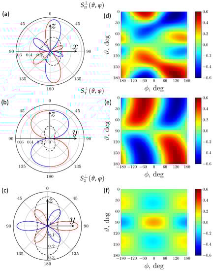
Figure 6.
(a,d) for electrons emitted in the plane (see Figure 5a); (b,e) for electrons emitted in the plane; (c,f) for electrons emitted in the plane. The photon energy corresponds to the resonance (19.78 eV). In (a,b), the phase between the harmonics was fixed at the value of ; in (c), it was fixed at the value of . Dashed black lines show that NPAD (arbitrary units are the same as in Figure 3a). Solid red (blue) lines correspond to positive (negative) spin components. In (d–f), the coherent control of the spin components is demonstrated (see text).
In the region of the 4s resonances, one of the two new components, , can reach similar values as with a large amplitude of the modulation of 0.6 when changing . At the same time, generally stays smaller than .
4. Conclusions
Spin polarization of photoelectrons has been considered in atomic ionization by linearly polarized light with the coherent sum of the fundamental frequency and its second harmonic for two beams polarized in the same and in orthogonal directions. It is demonstrated how violation of the symmetry of the + process leads to new components of the spin polarization. A possibility of coherent control on the spin polarization by manipulating the relative phase of the harmonics is demonstrated with numerical examples of photoionization of the neon atom in the region of the intermediate resonances. The variation of the spin polarization with the changing of the relative phase of the harmonics is quite large and can be of the order of unity.
Author Contributions
Conceptualization E.V.G. and A.N.G.-G.; investigation and formal analysis M.M.P.; resources and R-matrix calculations M.D.K.; funding acquisition E.V.G.; visualization M.M.P.; writing—original draft preparation M.M.P. and E.V.G.; writing—review and editing A.N.G.-G., E.V.G. and M.D.K. All authors have read and agreed to the published version of the manuscript.
Funding
M.M.P., M.D.K., and E.V.G. acknowledge support from the Foundation for the Advancement of Theoretical Physics and Mathematics BASIS via the Junior Leader program. The work of M.D.K. is also supported by the Ministry of Science and Higher Education of the Russian Federation (project No. 0818-2020-0005) with using resources of the Shared Services Center “Data Center of the Far-Eastern Branch of the Russian Academy of Sciences”.
Acknowledgments
The authors benefited greatly from discussions with Michael Meyer.
Conflicts of Interest
The authors declare no conflict of interest.
Appendix A. Statistical Tensor Formalism
Our approach is based on statistical tensor formalism [27,32]. The statistical tensor of spin is defined as
where () is the spin projection. is the spin density matrix, and standard notation for the Clebsch–Gordan coefficient is used. Below, we abbreviate .
The Cartesian components of electron spin polarization are related to the statistical tensors (A1) (given in the same coordinate system):
Because we are interested in dimensionless parameters of angular anisotropy and spin polarization, we do not normalize the density matrix and its trace is proportional to the ionization probability.
Components of statistical tensors of the electron spin, as a function of the electron emission angle, can be expanded in terms of spherical harmonics. We write it down in the coordinate system , associated with the electron emission:
where is the spherical harmonic dependent on the electron angular momentum l and its projection on the z-axis ; angles determine the direction of the electron emission.
are bilinear combinations of the ionization amplitudes, independent of the coordinate system. The meaning of the indices is the following: represents the number of photons absorbed in the first/second amplitude, and are determined by the photon polarization, i.e., for photons linearly polarized in direction, for photons linearly polarized in the direction .
We use the following abbreviations:
Here, E is the energy of the electron, is the energy of the initial state, is the scattering phase in the photoionization channel with orbital angular momentum l, is the total angular momentum of the final ion, J is the total angular momentum of the system ‘ion+electron’, is the total angular momentum of the intermediate state with energy , and standard notation for Clebsch–Gordan coefficients is used. The time-dependent factors are:
The dynamical parameters for each part of the statistical tensor (A5) are expressed in terms of the dipole matrix elements with
where
, standard notation for Wigner -symbols are used, and we introduced the multi-index . Permutation of the upper indices in (A12) or (A13) gives the relation . For single-photon ionization parameters, there are additional interrelations and .
The angle and spin integrated ionization probability does not depend on the orientation of the polarization vector
Performing the necessary transformations, we obtain:
- (a)
- For fields polarized in the same direction.
Angular distribution coefficients
Polarization coefficients
Leaving in Equations (A15)–(A23) only dynamical parameters or one obtains expressions for the two-photon or one-photon ionization, respectively.
- (b)
- For fields polarized in orthogonal directions.
Angular distribution coefficients
Polarization coefficients
Spin components in the laboratory system
Appendix B. Atomic Model
The ground state of Ne was obtained by a full self-consistent Hartree–Fock calculation of the configuration [33]. For the intermediate excited states, we first found the configuration state functions (CSFs) by self-consistent term-dependent calculations for each of the configurations (), (), , and with all possible terms. Then, we mixed all the obtained CSFs using the Breit–Pauli atomic Hamiltonian with full accounting of non-orthogonality of the electron orbitals [29]. Table A1 presents the intermediate states with the total angular momentum , which were taken into account in the calculations of the second-order amplitudes (summations over in Equations (A10)–(A13)). These wave functions were used also in the R-matrix calculations of the dipole matrix elements for transitions to the continuum. To obtain the ionic states (thresholds) in the R-matrix calculations, we first individually optimized each of the configurations from the lists:
- (a)
- odd CSFs: ; ; ; ; .
- (b)
- even CSFs: ; ; ; ; .
Then, we mixed them (for each of the two parities separately) similar to the atomic excited states and took the states
; ;
as the thresholds in the R-matrix calculations. Experimental energies of the thresholds are used [34].

Table A1.
Intermediate discrete states of neon with with their excitation energies [34] and leading LS-terms of the configuration decomposition.
Table A1.
Intermediate discrete states of neon with with their excitation energies [34] and leading LS-terms of the configuration decomposition.
| State | E, eV | Leading Configurations |
|---|---|---|
| 16.67 | ||
| 16.85 | ||
| 19.69 | ||
| 19.78 | ||
| 20.03 | ||
| 20.04 | ||
| 20.14 | ||
| 20.57 | ||
| 20.66 | ||
| 20.70 | ||
| 20.71 | ||
| 20.81 | ||
| 20.95 | ||
| 21.01 | ||
| 21.02 | ||
| 21.04 | ||
| 21.11 |
References
- Wolf, S.A.; Awschalom, D.D.; Buhrman, R.A.; Daughton, J.; von Molnar, S.; Roukes, M.L.; Chtchelkanova, A.; Treger, D. Spintronics: A spin-based electronics vision for the future. Science 2001, 294, 1488–1495. [Google Scholar] [CrossRef]
- Rougemaille, N.; Schmid, A. Magnetic imaging with spin-polarized low-energy electron microscopy. Eur. Phys. J. Appl. Phys. 2010, 50, 20101. [Google Scholar] [CrossRef]
- Johnson, P.D. Spin-polarized photoemission. Rep. Prog. Phys. 1997, 60, 1217–1304. [Google Scholar] [CrossRef]
- Heinzmann, U.; Dil, J.H. Spin-orbit-induced photoelectron spin polarization in angle-resolved photoemission from both atomic and condenced matter targets. J. Phys. Condens. Matter 2012, 24, 173001. [Google Scholar] [CrossRef] [PubMed]
- Lv, B.; Qian, T.; Ding, H. Angle-resolved photoemission spectroscopy and its application to topological materials. Nat. Rev. Phys. 2019, 1, 609–626. [Google Scholar] [CrossRef]
- Fano, U. Spin Orientation of Photoelectrons Ejected by Circularly Polarized Light. Phys. Rev. 1969, 178, 131–136, ibid 184, 250, 1969 Erratum. [Google Scholar] [CrossRef]
- Lubell, M.S.; Raith, W. Polarization Effect in Photoionization of Cesium. Phys. Rev. Lett. 1969, 23, 211–214. [Google Scholar] [CrossRef]
- Kessler, J.; Lorenz, J. Experimental Verification of the Fano Effect. Phys. Rev. Lett. 1970, 24, 87–88. [Google Scholar] [CrossRef]
- Cherepkov, N. Spin Polarization of Atomic and Molecular Photoelectrons. In Advances in Atomic and Molecular Physics; Bates, D., Bederson, B., Eds.; Academic Press: Cambridge, MA, USA, 1983; Volume 19, pp. 395–447. [Google Scholar] [CrossRef]
- Cherepkov, N. Spin polarisation of photoelectrons ejected from unpolarised atoms. J. Phys. B At. Mol. Opt. Phys. 2001, 12, 1279. [Google Scholar] [CrossRef]
- Cherepkov, N. Spin polarisation of electrons ejected from unpolarised atoms by unpolarised and linearly polarised light. J. Phys. B At. Mol. Opt. Phys. 1978, 11, L435. [Google Scholar] [CrossRef]
- Barth, I.; Smirnova, O. Spin-polarized electrons produced by strong-field ionization. Phys. Rev. A 2013, 88, 013401. [Google Scholar] [CrossRef]
- Milošević, D.B. Possibility of introducing spin into attoscience with spin-polarized electrons produced by a bichromatic circularly polarized laser field. Phys. Rev. A 2016, 93, 051402. [Google Scholar] [CrossRef]
- Milošević, D.B. Atomic and Molecular Processes in a Strong Bicircular Laser Field. Atoms 2018, 6, 61. [Google Scholar] [CrossRef]
- Liu, M.M.; Shao, Y.; Han, M.; Ge, P.; Deng, Y.; Wu, C.; Gong, Q.; Liu, Y. Energy- and Momentum-Resolved Photoelectron Spin Polarization in Multiphoton Ionization of Xe by Circularly Polarized Fields. Phys. Rev. Lett. 2018, 120, 043201. [Google Scholar] [CrossRef]
- Baranova, N.B.; Zel’dovich, B.Y. Physical effects in optical fields with nonzero average cube <E3> ≠ 0. J. Opt. Soc. Am. B 1991, 8, 27–32. [Google Scholar] [CrossRef]
- Yin, Y.Y.; Chen, C.; Elliott, D.S.; Smith, A.V. Asymmetric photoelectron angular distributions from interfering photoionization processes. Phys. Rev. Lett. 1992, 69, 2353–2356. [Google Scholar] [CrossRef]
- Goetz, R.E.; Koch, C.P.; Greenman, L. Quantum Control of Photoelectron Circular Dichroism. Phys. Rev. Lett. 2019, 122, 013204. [Google Scholar] [CrossRef]
- Prince, K.C.; Allaria, E.; Callegari, C.; Cucini, R.; Ninno, G.D.; Di Mitri, S.; Diviacco, B.; Ferrari, E.; Finetti, P.; Gauthier, D.; et al. Coherent control with a short-wavelength free-electron laser. Nat. Photonics 2016, 10, 176–179. [Google Scholar] [CrossRef]
- Callegari, C.; Grum-Grzhimailo, A.N.; Ishikawa, K.L.; Prince, K.C.; Sansone, G.; Ueda, K. Atomic, molecular and optical physics applications of longitudinally coherent and narrow bandwidth Free-Electron Lasers. Phys. Rep. 2021, 904, 1–59. [Google Scholar] [CrossRef]
- You, D.; Ueda, K.; Gryzlova, E.V.; Grum-Grzhimailo, A.N.; Popova, M.M.; Staroselskaya, E.I.; Tugs, O.; Orimo, Y.; Sato, T.; Ishikawa, K.L.; et al. New Method for Measuring Angle-Resolved Phases in Photoemission. Phys. Rev. X 2020, 10, 031070. [Google Scholar] [CrossRef]
- Gryzlova, E.V.; Popova, M.M.; Grum-Grzhimailo, A.N. Spin polarization of photoelectrons in bichromatic extreme-ultraviolet atomic ionization. Phys. Rev. A 2020, 102, 053116. [Google Scholar] [CrossRef]
- Hübner, J.; Rühle, W.W.; Klude, M.; Hommel, D.; Bhat, R.D.R.; Sipe, J.E.; van Driel, H.M. Direct Observation of Optically Injected Spin-Polarized Currents in Semiconductors. Phys. Rev. Lett. 2003, 90, 216601. [Google Scholar] [CrossRef]
- Stevens, M.J.; Smirl, A.L.; Bhat, R.D.R.; Najmaie, A.; Sipe, J.E.; van Driel, H.M. Quantum Interference Control of Ballistic Pure Spin Currents in Semiconductors. Phys. Rev. Lett. 2003, 90, 136603. [Google Scholar] [CrossRef]
- Gryzlova, E.V.; Popova, M.M.; Grum-Grzhimailo, A.N.; Staroselskaya, E.I.; Douguet, N.; Bartschat, K. Coherent control of the photoelectron angular distribution in ionization of neon by a circularly polarized bichromatic field in the resonance region. Phys. Rev. A 2019, 100, 063417. [Google Scholar] [CrossRef]
- Messiah, A. Quantum Mechanics; Dover Publications: Mineola, NY, USA, 1961. [Google Scholar]
- Balashov, V.V.; Grum-Grzhimailo, A.N.; Kabachnik, N.M. Polarization and Correlation Phenomena in Atomic Collisions. A Practical Theory Course; Physics of Atoms and Molecules, Kluwer Academic/Plenum Publishers: New York, NY, USA; Boston, MA, USA; Dordrecht, The Netherland; London, UK; Moscow, Russia, 2000. [Google Scholar] [CrossRef]
- Nakajima, T.; Lambropoulos, P. Electron spin-polarization in one-, two- and three-photon ionization of xenon. Europhys. Lett. 2002, 57, 25. [Google Scholar] [CrossRef]
- Zatsarinny, O. BSR: B-spline atomic R-matrix codes. Comput. Phys. Commun. 2006, 174, 273–356. [Google Scholar] [CrossRef]
- Jacobs, V.L. Polarization phenomena in multiphoton ionization of atoms. J. Phys. B Atom. Molec. Phys. 1973, 6, 1461–1472. [Google Scholar] [CrossRef]
- Dill, D. Resonances in Photoelectron Angular Distributions. Phys. Rev. A 1973, 7, 1976–1987. [Google Scholar] [CrossRef]
- Devons, S.; Goldfarb, L.J.B. Angular Correlations. In Kernreaktionen III/Nuclear Reactions III; Handbuch der Physik; Flügge, S., Ed.; Springer: Berlin/Heidelberg, Germany, 1957; Volume 42, Chapter 5; pp. 362–554. [Google Scholar] [CrossRef]
- Froese Fischer, C.; Brage, T.; Jönsson, P. Computational Atomic Structure. An MCHF Approach; Institute of Physics Publishing: Bristol, UK, 1997. [Google Scholar] [CrossRef]
- Kramida, A.; Ralchenko, Y.; Reader, J.; NIST ASD Team. NIST Atomic Spectra Database (ver. 5.8); National Institute of Standards and Technology: Gaithersburg, MD, USA, 2020. Available online: https://physics.nist.gov/asd (accessed on 21 April 2021).


Publisher’s Note: MDPI stays neutral with regard to jurisdictional claims in published maps and institutional affiliations. |
© 2021 by the authors. Licensee MDPI, Basel, Switzerland. This article is an open access article distributed under the terms and conditions of the Creative Commons Attribution (CC BY) license (https://creativecommons.org/licenses/by/4.0/).